statistical mechanics of self- gravitating n-body systems · 2018-08-05 · in classical...
TRANSCRIPT

Statistical mechanics of self-gravitating N-body systems
Tuesday, November 10, 15

gas in a box stellar system
molecules, m ~ 10-24 g stars, m ~ 1033 g
WIMPs, m ~ 10-22 g
N ~ 1023
N ~105 (globular clusters), ~105-1011 (stars in galaxies),~1065 (WIMPs in galaxies)
short-range forces long-range forces (gravity)
confined in a box confined by self-gravity
mean free path << system size (Knudsen number Kn << 1)
mean free path >> system size (Kn >> 1)
Tuesday, November 10, 15

K = kinetic energyW = potential energyE = K+W = total energy
virial theorem states that in a steady state
2K + W = E + K = 0 or E = −K.
In an isothermal gas K=3/2 NkT so heat capacity is
C= dE/dT = −3/2 Nk
which is negative
Tuesday, November 10, 15

• self-gravitating gas of mass M in a rigid spherical container of radius R
• solutions parametrized by density contrast Q = ρ(0)/ρ(R)
temperature
ener
gy
Q=3
Q=709
Q=32.1
Q=6.85
Tuesday, November 10, 15

• self-gravitating gas of mass M in a rigid spherical container of radius R
• solutions parametrized by density contrast Q = ρ(0)/ρ(R)
• heat capacity at constant volume C = dE/dT = slope
temperature
ener
gy
Q=3
Q=709
Q=32.1
Q=6.85
Antonov (1962)Lynden-Bell & Wood (1968)Thirring (1970)Katz (1978)
heat capacity > 0
heat capacity < 0
Tuesday, November 10, 15

• place box in contact with a heat bath at temperature T and slowly reduce T
• below Tmin there is no equilibrium state
temperature
ener
gy
Q=3
Q=709
Q=32.1
Q=6.85
Tmin
thought experiment # 1:
Tuesday, November 10, 15

• insulate box and suddenly expand its radius R
• E is conserved so if E<0 ER/(GM2) becomes more negative
• for R > Rmax there is no equilibrium state
• for Q > 709 all equilibrium states are unstable (entropy is a saddle point, not a maximum)
temperature
ener
gy
Q=3
Q=709
Q=32.1
Q=6.85
Rmax
thought experiment # 2:
• isolated self-gravitating systems have negative heat capacity• there is no thermodynamic equilibrium state for self-
gravitating systems unless they are enclosed in a sufficiently small box
Tuesday, November 10, 15

• isolated self-gravitating systems have negative heat capacity• there is no thermodynamic equilibrium state for self-
gravitating systems unless they are enclosed in a sufficiently small box
• there is no “heat death” of the Universe
Tuesday, November 10, 15

• there is no thermodynamic equilibrium state for self-gravitating systems unless they are enclosed in a sufficiently small box ⇒ stellar systems cannot survive much longer than the equipartition or relaxation time due to gravitational encounters between stars
• for a spherical system of N stars with crossing or orbital time tcross
where R and V are the typical size and velocity of the stellar system
• roughly, an N-body system survives for about N crossing times
Tuesday, November 10, 15

globular clusters N ≃ 105 ✔ ︎
solar neighborhood N ≃ 105 ✘
dark-matter halos N ≃ 1011 to 1065 ✘
planetary systems N ≃ a few ✔ ︎ ( !?)
Milky Way nuclear star cluster
N ≃ 105 ✔ ( !?)
Tuesday, November 10, 15

globular clusters:
N ≃ 105
tcross ≃ 106 yr trelax ≃ 1010 yr
Tuesday, November 10, 15

globular clusters:
N ≃ 105
tcross ≃ 106 yr trelax ≃ 1010 yr • core collapse
• equipartition and evaporation• gravothermal oscillations• Fokker-Planck approximation• soft and hard binaries • tidal shocks• dynamical friction
Aarseth, Ambartsumian, Baumgardt, Cohn, Giersz, Goodman, Heggie, Hénon, Hut, Kulsrud, Larson, Lee, Lightman, Makino, Quinlan, Rasio, Shapiro, Spitzer, Spurzem, Stodółkiewicz, Sugimoto,Takahashi, etc.
Tuesday, November 10, 15

the solar neighborhood:
tcross ≃ 108 yr trelax ≃ 1013 yr
10 pc
Tuesday, November 10, 15

} } Jeans (1928)
• stars in the Milky Way disk exhibit velocity dispersion of 5-50 km/s in addition to common rotational velocity of ~220 km/s
• more massive stars have smaller random velocities, consistent with equipartition
• timescale required to reach equipartition due to gravitational encounters between stars is ~1013 yr ⇒ universe must be at least this old
Tuesday, November 10, 15

• stars in the Milky Way disk exhibit velocity dispersion of 5-50 km/s in addition to common rotational velocity of ~220 km/s
• more massive stars have smaller random velocities, consistent with equipartition
• timescale required to reach equipartition due to gravitational encounters between stars is ~1013 yr ⇒ universe must be at least this old
• in fact random velocities arise from gravitational interactions with interstellar clouds and spiral arms, and more massive stars have smaller velocities because they are younger
Jeans (1928)
Tuesday, November 10, 15
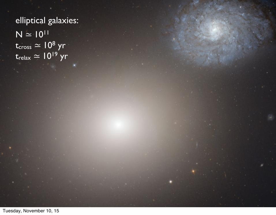
elliptical galaxies:
N ≃ 1011
tcross ≃ 108 yr trelax ≃ 1019 yr
Tuesday, November 10, 15

• the distribution of stars is similar, apart from scale, in all galaxies (Sérsic profile)
• the distribution of stellar velocities is close to Maxwellian• how is this achieved if the relaxation time is much longer than the age?
— the “fundamental paradox of stellar dynamics” (Ogorodnikov 1965)
Answer: • large-scale fluctuations in the mean gravitational field during collapse of
the galaxy drive the distribution of stars towards an (approximately) universal form (“violent relaxation”, Lynden-Bell 1967)
elliptical galaxies:
N ≃ 1011
tcross ≃ 108 yr trelax ≃ 1019 yr
Tuesday, November 10, 15

Tuesday, November 10, 15

Tuesday, November 10, 15

• density profiles of dark-matter halos in simulations are well fit over > 3 orders of magnitude in radius, > 5 orders of magnitude in mass, and a wide variety of initial conditions by simple empirical formulae
• e.g., Navarro-Frenk-White (NFW) profile
N-body simulations,Navarro et al. (2004)
Tuesday, November 10, 15

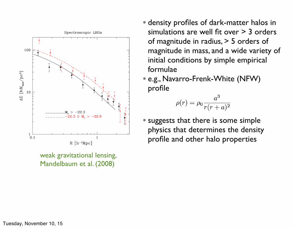
• density profiles of dark-matter halos in simulations are well fit over > 3 orders of magnitude in radius, > 5 orders of magnitude in mass, and a wide variety of initial conditions by simple empirical formulae
• e.g., Navarro-Frenk-White (NFW) profile
weak gravitational lensing,Mandelbaum et al. (2008)
Tuesday, November 10, 15
• density profiles of dark-matter halos in simulations are well fit over > 3 orders of magnitude in radius, > 5 orders of magnitude in mass, and a wide variety of initial conditions by simple empirical formulae
• e.g., Navarro-Frenk-White (NFW) profile
• suggests that there is some simple physics that determines the density profile and other halo properties
weak gravitational lensing,Mandelbaum et al. (2008)
Tuesday, November 10, 15

• density profiles of dark-matter halos in simulations are well fit over > 3 orders of magnitude in radius, > 5 orders of magnitude in mass, and a wide variety of initial conditions by simple empirical formulae
• e.g., Navarro-Frenk-White (NFW) profile
• suggests that there is some simple physics that determines the density profile and other halo properties
Lynden-Bell (1967)Saslaw (1968, 1969,1970)Shu (1969,1978,1987)Lecar & Cohen (1971)Miller (1972)Severne & Luwel (1980)Binney (1982)Rephaeli (1983)Madsen (1987)Stiavelli & Bertin (1987)White & Narayan (1987)Kandrup (1989)Soker (1990,1996)Hjorth & Madsen (1991,1993)Chavanis (1998,2002,2006)Ascasibar et al. (2004)Arad et al. (2004)Hansen et al. (2005,2010)Arad & Lynden-Bell (2005)Lu et al. (2006)Valluri et al. (2007)Williams & Hjorth (2010)Dalal et al. (2010)Visbal et al. (2012)Pontzen & Governato (2013)Beraldo e Silva et al. (2014) Alard (2014)
Tuesday, November 10, 15

Boltzmann entropy
Tuesday, November 10, 15

✗Boltzmann entropy
Tuesday, November 10, 15

The primary feature of entropy in statistical mechanics is that it satisfies Boltzmann’s H theorem, i.e. molecular collisions imply that
This calculation is based on several strong assumptions:• instantaneous binary collisions• short-range forces• molecular chaos
What kind of H-theorem applies to violent relaxation?
Boltzmann entropy
Tuesday, November 10, 15

Most general approach is to treat relaxation is a Markov process in phase space defined by the probability pji that a particle in cell i at the initial time transitions to cell j at the final time. If all cells have the same size then time-reversibility implies pji = pij. Then one can show
In this process the Boltzmann entropy has no special status. There is a different “entropy” for every convex function and all must go up.
Boltzmann entropy
Tuesday, November 10, 15

An initial phase-space distribution f(x,v) can only evolve into a final one f′(x,v) if all possible H-functions are smaller for f′ than for f.
Simpler criteria exist (Tremaine, Hénon & Lynden-Bell 1987, Yu & Tremaine 2002, Dehnen 2005)
In classical statistical mechanics, relaxation leads to a unique equilibrium distribution function f(x,v)
Violent relaxation leads to a partial ordering of distribution functions f(x,v)
Tuesday, November 10, 15

An initial phase-space distribution f(x,v) can only evolve into a final one f′(x,v) if all possible H-functions are smaller for f′ than for f.
Simpler criteria are given by Tremaine, Hénon & Lynden-Bell (1987), Yu & Tremaine (2002), and Dehnen (2005)
Dehnen (2005)
Unfortunately for cold dark matter the left side diverges...⇒ some physics other than maximum entropy is needed to understand violent relaxation
In classical statistical mechanics, relaxation leads to a unique equilibrium distribution function f(x,v)
Violent relaxation leads to a partial ordering of distribution functions f(x,v)
Tuesday, November 10, 15

Statistical mechanics of planetary systems
There are many bad examples of attempts to explain the spacing and other properties of planetary orbits from first principles
Nevertheless there are reasons to try again:• Kepler has provided a large statistical sample of multi-planet systems
• N-body integrations can routinely follow the evolution of systems for 100 Myr
• there are hints of interesting behavior from studies of the solar system:
- the orbits of the planets in the solar system are chaotic, with Liapunov (e-folding) times of ~107 yr (Sussman & Wisdom 1988, 1992, Laskar 1989, Hayes 2008)
- the outer solar system is “full” in the sense that no stable orbits remain between Jupiter and Neptune (Holman 1997)
- there is a 1% chance that Mercury will be lost from the solar system before the end of the Sun’s life in ~ 7 Gyr
These suggest that some properties of the solar system might be determined by the statistical mechanics of orbital chaos
Tuesday, November 10, 15

eccentricity of Mercury for 2500 nearby initial conditions
Laskar & Gastineau (2009)
Tuesday, November 10, 15

The last stages of terrestrial planet formation
• the accretion of planetesimals leads to a few dozen “planetary embryos” of similar size
• eccentricities of the embryos remain small because they are damped by dynamical friction from residual population of small planetesimals
• eventually the small planetesimals disappear
• surviving embryos gradually excite one another's eccentricities until their orbits cross and they collide
• through collisions, the number of surviving bodies slowly declines until we are left with a small number of planets on well-separated, stable orbits (late-stage accretion, post-oligarchic growth, giant-impact phase)
•maybe the giant-impact phase tends to produce an ensemble of planetary systems with statistically similar properties
Tuesday, November 10, 15

Maybe the giant-impact phase tends to produce an ensemble of planetary systems with statistically similar properties. This idea is not new:• Laskar (1996): “maybe there was some extra planet at the early stage of formation of
the solar system...but this led to so much instability that one of the planets...suffered a close encounter or a collision. This leads eventually to the escape of the planet and the remaining system gets more stable...at each stage, the system should have a time of stability comparable with its age.”
• Barnes & Raymond (2004): proposed the packed planetary systems hypothesis: “many systems lie on the verge of instability. Planetary systems near instability are as tightly packed as possible; there is no room for additional companions.”
• Malhotra (2015): “as a consequence of mergers or ejections of planets, the surviving planets undergo a random walk of their orbits; unstable configurations are steadily winnowed.”
• Volk & Gladman (2015): “systems of tightly packed inner planets initially surrounded nearly all such stars and those observed are the final survivors of a process in which long-term metastability eventually ceases and the systems proceed to collisional consolidation or destruction”
• Pu & Wu (2015): “we suggest that typical planetary systems were formed with even tighter spacing, but most, except for the widest ones, have undergone dynamical instability, and are pared down to a more anemic version of their former selves, with fewer planets and larger spacings.”
Tuesday, November 10, 15

Statistical mechanics of planetary systems
The range of strong interactions from a planet of mass m orbiting a star of mass M in a circular orbit of radius a is the Hill radius
Numerical integrations show that planets of mass m, m′ with semi-major axes a, a’, a < a’ are stable for N orbital periods if closest approach exceeds k Hill radii, or
typically k(1010) ≃ 11 ± 1
Pu & Wu (2014)
Ansatz: planetary systems fill uniformly the region of phase space allowed by stability (~ ergodic hypothesis)
Tuesday, November 10, 15

Statistical mechanics of planetary systems
1. Ansatz: planetary systems fill uniformly the region of phase space allowed by stability
2. Work in the sheared sheet model, which replaces usual Keplerian disk by a rectangular box with shear (not essential, but eliminates spatial gradients and other complications)
Leads to an N-planet distribution function
For comparison the distribution function for a one-dimensional gas of hard rods of length L (Tonks 1936) is
In both systems the partition function depends only on the filling factor
}
phase-space volumeapocenter and pericenter must be separated by k Hill radii
step function
Tuesday, November 10, 15

Statistical mechanics of planetary systems
N-planet distribution function
Work with the grand canonical ensemble, i.e., assume each planetary system is a subsystem with variable number of planets
Predictions:
• eccentricity distribution:
where τ is a free parameter determined by the filling factor
Tuesday, November 10, 15

e.g., N-body simulations of planet growth by Hansen & Murray (2013)
τ = 0.060 ± 0.003
Tuesday, November 10, 15

Statistical mechanics of planetary systems
N-planet distribution function
Work with the grand canonical ensemble.
Predictions:
• eccentricity distribution• distribution of semi-major axis differences between nearest neighbors:
✔ ︎ with one free parameter
Tuesday, November 10, 15

e.g., N-body simulations of planet growth by Hansen & Murray (2013)
τ = 0.060 ± 0.003
Tuesday, November 10, 15

Statistical mechanics of planetary systems
N-planet distribution function
Work with the grand canonical ensemble.
Predictions:
• eccentricity distribution• distribution of semi-major axis differences
✔ ︎ with one free parameter✔ ︎ with no free parameters
Tuesday, November 10, 15
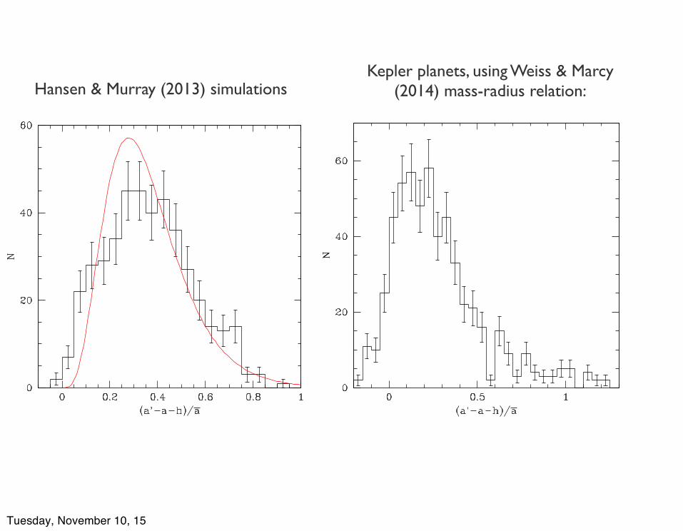
Kepler planets, using Weiss & Marcy (2014) mass-radius relation:Hansen & Murray (2013) simulations
Tuesday, November 10, 15

Kepler planets, using Weiss & Marcy (2014) mass-radius relation:Hansen & Murray (2013) simulations
Tuesday, November 10, 15

Kepler planets, using Weiss & Marcy (2014) mass-radius relation:Hansen & Murray (2013) simulations
convolve theoretical distribution with the scatter in the estimate of the Hill radii using Weiss & Marcy (2014)
mass-radius relation, σ(rH)/rH=0.4
Tuesday, November 10, 15

Kepler planets, using Weiss & Marcy (2014) mass-radius relation:
τ = 0.03
}missing planets?
Tuesday, November 10, 15
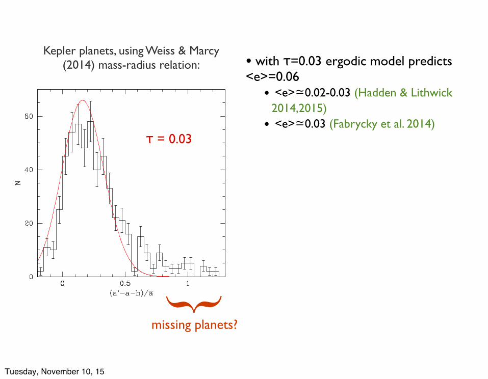
Kepler planets, using Weiss & Marcy (2014) mass-radius relation:
τ = 0.03
• with τ=0.03 ergodic model predicts <e>=0.06
• <e>≃0.02-0.03 (Hadden & Lithwick 2014,2015)
• <e>≃0.03 (Fabrycky et al. 2014)
}missing planets?
Tuesday, November 10, 15

Kepler planets, using Weiss & Marcy (2014) mass-radius relation:
τ = 0.03
• with τ=0.03 ergodic model predicts <e>=0.06
• <e>≃0.02-0.03 (Hadden & Lithwick 2014,2015)
• <e>≃0.03 (Fabrycky et al. 2014)
}missing planets?
• ergodic model predicts no correlation between mass and eccentricity in a given system
Tuesday, November 10, 15

1 2 3 4 5 6 7 8 9 10 1210−2
10−1
100
Number of Planets
Ecce
ntric
ity
Median EccentricityPower Law Fit to Systemswith Multiplicity > 3
Student Version of MATLAB
2!
e(M) ⇡ 0.584M �1.20
Med
ian
Ecce
ntric
ity!
SS!
• ergodic model predicts <e> ~ 1/N
Limbach & Turner (2014)
missing planets?
Tuesday, November 10, 15

5
and then later ‘adaptive optics’ (AO: correcting the wave distortions on-line) became available, which have since allowed increasingly precise high resolution near-infrared observations with the currently largest (10 m diameter) ground-based telescopes of the Galactic Center (and nearby galaxy nuclei).
10”(0.4 pc)
VLT: H (1.6Pm) - L’(3.8Pm)VLA: 1.3cm
Figure 2. Near-infrared/radio, color-composite image of the central light years of Galactic Center. The blue and green colors represent the 1.6 and 3.8µm broad band near-infrared emission, at the diffraction limit (~0.05”) of the 8m Very Large Telescope (VLT) of the European Southern Observatory (ESO), and taken with the ‘NACO’ AO-camera and an infrared wavefront sensor (adapted from Genzel et al. 2003). Similar work has been carried out at the 10 m Keck telescope (Ghez et al. 2003, 2005). The red color image is the 1.3cm radio continuum emission taken with the Very Large Array (VLA) of the US National Radio Astronomy Observatory (NRAO). The compact red dot in the center of the image is the compact, non-thermal radio source SgrA*. Many of the bright blue stars are young, massive O/B- and Wolf-Rayet stars that have formed recently. Other bright stars are old, giants and asymptotic giant branch stars in the old nuclear star cluster. The extended streamers/wisps of 3.8µm emission and radio emission are dusty filaments of ionized gas orbiting in the central light years (adapted from Genzel, Eisenhauer & Gillessen 2010).
Early evidence for the presence of a non-stellar mass concentration of 2-4 million times the mass of the Sun (M
�) came from mid-infrared imaging spectroscopy of the
12.8µm [NeII] line, which traces emission from ionized gas clouds in the central parsec region (Wollman et al. 1977, Lacy et al. 1980, Serabyn & Lacy 1985). However, many
the nuclear star cluster at the Galactic center:
N ≃ 105 stars plus a black hole of 4 × 10⁶ M⦿tcross ≃ 1 to 104 yr trelax ≃ 109 yr
Genzel (2015)
with Bence Kocsis (IAS and Eötvös University)
Tuesday, November 10, 15

Bartko et al. (2009) blue = clockwise rotation (61 stars)
red = counter-clockwise rotation (29 stars)
• ~ 100 massive young stars found in the central parsec
• age 6 Myr; implied star-formation rate is so high that it must be episodic
• line-of-sight velocities measured by Doppler shift and angular velocities measured by astrometry (five of six phase-space coordinates)
• velocity vectors lie close to a plane, implying that many of the stars are in a disk (Levin & Beloborodov 2003)
• there is strong evidence for a second disk co-spatial with the first but roughly perpendicular to it
The stellar disk(s) in the Galactic center
1 pc = 25”
Tuesday, November 10, 15

• plots show probability distribution of orbit normals of the young stars
Bartko et al. (2009)
0.15-0.3 pc
0.3-0.5 pc
0.05-0.15 pc
64°
• clockwise disk: • warped (best-fit normals in inner and outer image differ by 64°)
• disk is less well-formed at larger radii• counter-clockwise disk:
• weaker evidence • localized between 0.1 and 0.3 pc
•disks are embedded in a spherical cluster of old, fainter stars with M(0.1 pc) ~ 1×10⁵ M⊙ compared to M・ = 4×10⁶ M⊙
1 pc = 25”
Tuesday, November 10, 15

Resonant relaxation
• inside ~0.5 pc gravitational field is dominated by the black hole (Mstars < 105 M⊙, M● ~ 4×10⁶ M⊙) and therefore is nearly spherical
• on timescales longer than the apsidal precession period each stellar orbit can be thought of as a disk or annulus
• each disk exerts a torque on all other disks
• mutual torques can lead to relaxation of orbit normals or angular momenta
• energy (semi-major axis) and scalar angular momentum (or eccentricity) of each orbit is conserved, but orbit normal is not
Rauch & Tremaine (1996)
Tuesday, November 10, 15

Interaction energy between stars i and j is mimjf(ai,aj,ei,ej,cos µij) where µij is the angle between the orbit normals
massessemi-major axes
eccentricities
Simplify this drastically by assuming equal masses, equal semi-major axes, circular orbits, and neglecting all harmonics other than quadrupole
Resulting interaction energy between two stars i and j is just
- C cos2 µij
where µij is the angle between the two orbit normals ni and nj
Resonant relaxation
Maier-Saupe model
Toy model:
Tuesday, November 10, 15

Resonant relaxation
Interaction energy between two stars is
H = -C cos2 µ
where µ is the angle between the two orbit normals
• 800 stars
• each point represents tip of orbit normal
• orbit normals initially in northern hemisphere are yellow, south is red
animation by B. Kocsis
Tuesday, November 10, 15

animation by B. Kocsis
Tuesday, November 10, 15

• integrate orbit-averaged equations of motion• yellow = disk stars, blue-red = stars in
spherical cluster, colored by increasing radius • large yellow = molecular torus • direction and radius of each point
represents direction of angular-momentum vector and semi-major axis of star• 32K stars • each point represents tip of orbit
normal
animation by B. Kocsis
Tuesday, November 10, 15

animation by B. Kocsis
Tuesday, November 10, 15
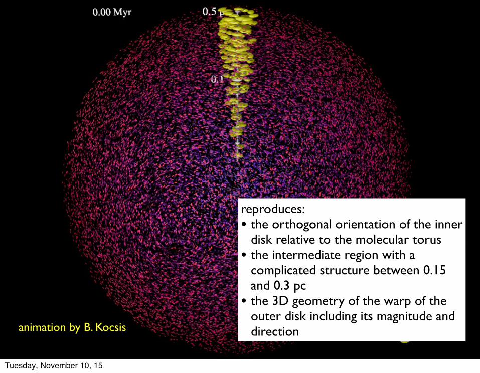
animation by B. Kocsis
reproduces:• the orthogonal orientation of the inner
disk relative to the molecular torus• the intermediate region with a
complicated structure between 0.15 and 0.3 pc
• the 3D geometry of the warp of the outer disk including its magnitude and direction
Tuesday, November 10, 15

“All models are wrong, but some are useful”Box & Draper (1987)
Tuesday, November 10, 15

Tuesday, November 10, 15