static and dynamic quantization in model-based networked ...pantsakl/publications/347-ijc07.pdf ·...

International Journal of ControlVol. 80, No. 1, January 2007, 87–101

Static and dynamic quantization in model-basednetworked control systems

L. A. MONTESTRUQUE*y and P. J. ANTSAKLISz

yEmNet, LLC; 12441 Beckley St., Granger, IN 46530, USAzDepartment of Electrical Engineering, University of Notre Dame,

Notre Dame, IN 46556, USA

(Received 10 August 2005; in final form 21 July 2006)

In this paper the effects of quantization in an important class of networked control systems

called model-based networked control systems (MB-NCS) are considered. The MB-NCS

architecture uses an explicit model of the plant in the controller in order to reduce the network

traffic, while attempting to prevent excessive performance degradation. Sufficient stability

conditions for two types of static and a dynamic quantization schemes for MB-NCS are

derived. An important feature is that the stability conditions are explicitly expressed in terms

of the plant and controller dynamics, the error between the model and the plant parameters,

the transmission or update times, the quantization parameters, and a robustness measure of

the system to parameter uncertainty. This is important because it allows the design of the

controller and network parameters to achieve the desired goals. Examples are used throughout

to illustrate the main results.

1. Introduction

A networked control system (NCS) is a control systemin which a data network is used as feedback media. NCSis an important area see for example Walsh et al. (1999),Nair and Evans (2000), Yook et al. (2002) andNetworked Control Systems Sessions (2003). Industrialcontrol systems are increasingly using networks as mediato interconnect the different components. However, theuse of networked control systems poses some challenges.One of the main problems to be addressed whenconsidering a networked control system is the size ofbandwidth required by each subsystem. Since eachcontrol subsystem must share the same medium thereduction of the individual bandwidth is a majorconcern. Two ways of addressing this problem are:minimizing the frequency of transfer of informationbetween the sensor and the controller/actuator; orcompressing or reducing the size of the data transferredat each transaction. Shared characteristics amongpopular digital industrial networks are the smalltransport time and big overhead per packet, thus using

fewer bits per packet has small impact over the overall

bit rate. So reducing the rate at which packets are

transmitted brings better benefits than data compression

in terms of bit rate used. The MB-NCS architecture

makes explicit use of knowledge about the plant

dynamics to enhance the performance of the system.

MB-NCS were introduced in Montestruque and

Antsaklis (2002a) (also see Montestruque and

Antsaklis (2004).Previously we have assumed that the network is

capable of transporting data with infinite precision.

For example, for the state feedback MB-NCS it is

assumed that the sensor sends the exact value of the

state over the network to the controller/actuator. This is

of course not possible with digital networks since the

length of each data packet is finite. It was claimed that,

since a large portion of standard industrial networks

implement a large number of bits available to represent

data, the error between the quantized value and the

actual value was negligible. Even when this is so, we

want to study the effect of these quantization errors on

the system stability.Several results have been published regarding quanti-

zation issues in NCS and sampled data problems*Corresponding author. Email: [email protected]

International Journal of ControlISSN 0020–7179 print/ISSN 1366–5820 online � 2007 Taylor & Francis

http://www.tandf.co.uk/journalsDOI: 10.1080/00207170600931663

(Bamieh 1996, Liberzon and Brockett 2000, Nair and

Evans 2000a, b, Elia and Mitter 2001, Fagnani and

Zampieri 2002, Hespanha et al. 2002, Fu 2003, Liberzon

2003a, b, Nair et al. 2003 and Ling and Lemmon 2004).

Most results attempt to characterize the stability

properties of NCS when the number of bits used by

each network packet is finite and small. The main thrust

for this research is the need to reduce the amount

of bandwidth necessitated by a NCS so that a larger

amount of NCS can share the network. The goal with

MB-NCS is also the reduction of bandwidth, but the

design of the MB-NCS first attempts to reduce the

bandwidth by reducing the rate at which packets are sent

(Montestruque and Antsaklis 2002a). A second step is

to further reduce the bandwidth by reducing the number

of bits used to transmit each packet. This allows the

designer to consider several design parameters in a

sequential fashion. Specifically, a stable non-quantized

MB-NCS must be designed first using previous results

(Montestruque and Antsaklis 2002a). Then, the effect of

quantization can be assessed using the results in this

paper. In this way the designer has at her disposal a

number of parameters that can be modified, namely the

packet transmission times and the number of bits used

for each packet. Sufficient conditions on the control

system stability can be given depending on bounds over

the model uncertainty.In this paper stability conditions for MB-NCS under

popular quantization schemes are derived. Both static

quantizers and dynamic quantizers are considered.

Static quantizers have quantization schemes that do

not vary with time, that is the error between the

quantized value and the real value does not depend on

time. Two quantizers of this type are considered: the

uniform quantizer with a constant maximum quantiza-

tion error; and the logarithmic quantizer with a

maximum quantization error that is proportional to

the norm of the quantized value. Dynamic quantizers

dynamically adjust their quantization regions to com-

pensate for uncertainties while giving a quantization

error that shrinks with time.The main contributions of this paper are the results

on stability of quantized MB-NCS that show the explicit

dependence on the update time, the control law,

the model dynamics, the quantization parameters, and

the difference between the model and plant dynamics. In

x 2 the basic MB-NCS setup is reviewed for complete-

ness. Stability of MB-NCS with no quantization and

periodic transmissions are considered. In x 3 the stability

of MB-NCS with two types of static quantizers

are studied, namely the uniform quantizer and the

logarithmic quantizer. The stability of MB-NCS with

a dynamic quantizer is studied in x 4. Conclusions are

given in x 5.

2. Stability of a state feedback linear MB-NCS

We consider the control of a continuous linear plant

where the state sensor is connected to a linear controller/

actuator via a network. In this case, the controller uses

an explicit model of the plant that approximates the

plant dynamics and makes possible the stabilization

of the plant even under slow network conditions.In this section we determine conditions under which

the transfer time between the sensor and the controller/

actuator results in a stable control system. An approx-

imate model of the plant is used in the controller/

actuator side to estimate the actual value of the plant

state vector, in this way the sensor can delay the

transmission of update information about the plant

state. The main idea is to perform the feedback by

updating the model’s state using the actual state of the

plant that is provided by the sensor. The rest of the time

the control action is based on a plant model that is

incorporated in the controller/actuator and is running

open loop for a period of h seconds. The control

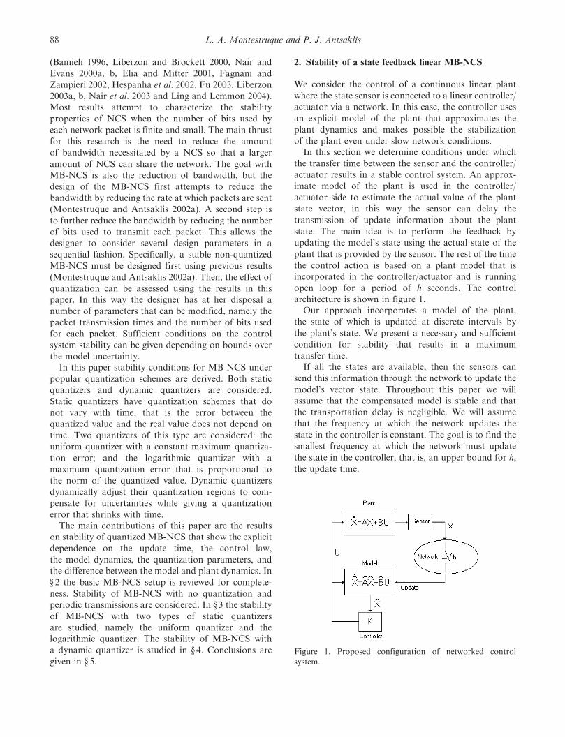
architecture is shown in figure 1.Our approach incorporates a model of the plant,

the state of which is updated at discrete intervals by

the plant’s state. We present a necessary and sufficient

condition for stability that results in a maximum

transfer time.If all the states are available, then the sensors can

send this information through the network to update the

model’s vector state. Throughout this paper we will

assume that the compensated model is stable and that

the transportation delay is negligible. We will assume

that the frequency at which the network updates the

state in the controller is constant. The goal is to find the

smallest frequency at which the network must update

the state in the controller, that is, an upper bound for h,

the update time.

Figure 1. Proposed configuration of networked controlsystem.

88 L. A. Montestruque and P. J. Antsaklis

Consider the control system of figure 1 where theplant is given by _x ¼ Axþ Bu, the plant model by_x ¼ Axþ Bu, and the controller by u ¼ Kx. The stateerror is defined as e ¼ x� x, and represents thedifferences between the plant state and the modelstate. The modelling error matrices A¼A� A and~B ¼ B� B represent the difference between the plantand the model. Also define the state erroreðtÞ ¼ xðtÞ � xðtÞ and

� ¼Aþ BK �BK~Aþ ~BK A� ~BK

� �:

A necessary and sufficient condition for stability of thestate feedback MB-NCS is now presented.

Theorem 1 (Montestruque and Antsaklis 2003): TheState Feedback MB-NCS is globally exponentially stablearound the solution z¼ [xT� eT]T¼ 0 if and only if theeigenvalues of

I 00 0

� �e�h I 0

0 0

� �

are strictly inside the unit circle.

It can be shown (Montestruque 2004) that theeigenvalues of

M ¼I 00 0

� �e�h I 0

0 0

� �

are inside the unit circle if and only if the eigenvalues ofN ¼ eðAþBKÞh þ�ðhÞ with �ðhÞ ¼ eAh

R h0 e�A�ð ~Aþ ~BKÞ �

eðAþBKÞ�d� are inside the unit circle. Observe that the

eigenvalues of the compensated model appear in the firstterm of N and that the second term �(h) can be madesmall by having small update times h or small modellingerror. A detailed proof for Theorem 1 can be found inMontestruque and Antsaklis (2002a or 2002b).

Example 1: In real applications uncertainty can fre-quently be expressed as tolerances over the differentmeasured parameter values of the plant. This can bemapped into structured or parametric uncertaintieson the state space matrices. Next an example is givenon how Theorem 1 can be applied if two entries onthe A matrix of the model can vary within a certaininterval

model: A ¼0 0

0 1

" #, B ¼

0

1

" #;

plant: A ¼0 1þ ~a12

0þ ~a21 0

" #, B ¼

0

1

" #;

with ~a12 ¼ ½�0:5, 0:5�, ~a21 ¼ ½�0:5, 0:5�

controller: K ¼ ½�1, � 2�:

The system will now be tested for an update time ofh¼ 2.5 seconds. The following contour plot in figure 2represents the maximum eigenvalue magnitude for thetest matrix M as a function of the (1, 2) and (2, 1)entries possible values. Here the contours at height equalto one are relevant to stability. It is easy to isolatethe stable and unstable regions in the uncertaintyparameter plane. The stable region is between the lineslabelled as 1.

Figure 2. Contour plot maximum eigenvalue magnitude vs model error.

Static and dynamic quantization 89

3. Stability of MB-NCS with static quantization

In this section we address the stability analysis of a statefeedback MB-NCS using a static quantizer. Staticquantizers have defined quantization regions that donot change with time. They are an important class ofquantizers since they are simple to implement in eitherhardware or software and are not as computationallyexpensive as their dynamic counterparts. Two types ofquantizers are analysed here, namely uniform quantizersand logarithmic quantizers. Each quantizer is associatedwith two popular data representations. The uniformquantizer is associated with the fixed-point datarepresentation. Indeed, fixed-point numbers have aconstant maximum error regardless of how close is theactual number to the origin. Logarithmic quantizers onthe other hand are associated with floating-pointnumbers, this allows the maximum error to decrease asthe actual number is close to origin.

3.1 State feedback MB-NCS with uniform quantization

Let a uniform quantizer be described by a functionq : Rn ! Rn with the following property:

z� q zð Þ�� , z 2 Rn, � > 0: ð1Þ

Theorem 2: Assume that the networked system withoutquantization is stable and satisfies

eðAþBKÞTh þ�ðhÞT� �

P eðAþBKÞh þ�ðhÞ� �

� P ¼ �QD

ð2Þ

with P and QD symmetric and positive definite. Then whenusing the uniform quantizer defined by (1), the statefeedback MB-NCS plant state will enter and remain in theregion kxk�R defined by

R ¼ e ��ðAþBKÞh þ�maxðhÞ� �

rþ e ��ðAÞh þ�maxðhÞ� �

�

where r ¼

ffiffiffiffiffiffiffiffiffiffiffiffiffiffiffiffiffiffiffiffiffiffiffiffiffiffiffiffiffiffiffiffiffiffiffiffiffiffiffiffiffiffiffiffiffiffiffiffiffiffiffiffiffiffiffiffiffiffiffiffiffiffiffiffiffiffiffiffiffiffiffiffiffiffiffilmaxððeAh ��ðhÞÞTPðeAh ��ðhÞÞTÞ�2

lminðQDÞ

s

and �maxðhÞ ¼

Z h

0

e ��ðAÞðh��Þ ��ð ~Aþ ~BKÞe ��ðAþBKÞ�d�:

Proof: The response for the error is given now by

eðtÞ ¼ eAðt�tkÞeðtkÞ þ�ðt� tkÞx tþk� �

¼ eAðt�tkÞeðtkÞ þ�ðt� tkÞðxk � eðtkÞÞ

¼ eAðt�tkÞ ��ðt� tkÞ� �

eðtkÞ þ�ðt� tkÞxk ð3Þ

where

�ðt� tkÞ ¼

Z t�tk

0

eAðt�tk��Þð ~Aþ ~BKÞeðAþBKÞ�d�:

Note that since there is non zero quantization error, theinitial value for the error e(tk) is no longer zero as it wasin the case for non-quantized MB-NCS. Moreover thecontribution due to this initial value for the error willgrow exponentially with time and with a rate thatcorresponds to the uncompensated plant dynamics.So at time t 2 ½tk, tkþ1� the plant state is

xðtÞ ¼ xðtÞ þ eðtÞ

¼ eðAþBKÞðt�tkÞxk þ eAðt�tkÞ ��ðt� tkÞ� �

eðtkÞ

þ�ðt� tkÞxk: ð4Þ

We can therefore evaluate a Lyapunov functionV¼xTPx at any instant in time t 2 ½tk, tkþ1�. It isknown that for uniformly exponential stability werequire (Ye et al. 1998) that

1

hVðxðtkþ1ÞÞ � VðxðtkÞÞð Þ � �c jjxðtkÞjj

2� �

, c 2 Rþ: ð5Þ

We are interested in the value of the Lyapunov functionV at tkþ1

Vðxðtkþ1ÞÞ ¼ xðtkþ1ÞTPxðtkþ1Þ

¼ xTk eðAþBKÞh þ�ðhÞ� �T


xk

þ eTk ðeAh ��ðhÞÞTPðeAh ��ðhÞÞek ð6Þ

where

h ¼ hk ¼ tkþ1 � tk > 0, ek ¼ eðtkÞ:

So we obtain

Vðxðtkþ1ÞÞV xðtkÞð Þ

¼ xTk eðAþBKÞh þ�ðhÞ� �T


xk

þ eTk eAh ��ðhÞ� �T

P eAh ��ðhÞ� �

ek � xTkPxk

¼ eTk eAh ��ðhÞ� �T

P eAh ��ðhÞ� �

ek � xTkQDxk: ð7Þ

Note that we can compute eAh��(h) as follows:

eAh ��ðhÞ ¼ I 0

e

A ~Aþ ~BK

0 AþBK

� �ðt�tk Þ

0BB@

1CCA I

�I

� �: ð8Þ


We can bound (7) by

eTk ðeAh ��ðhÞÞTPðeAh ��ðhÞÞek � xTkQDxk

� lmax ðeAh ��ðhÞÞTPðeAh ��ðhÞÞ� �

�2 � lminðQDÞjjxkjj2:

ð9Þ

The sampled value of the state of the plant at the updatetimes will enter the region kxk� r where

r ¼

ffiffiffiffiffiffiffiffiffiffiffiffiffiffiffiffiffiffiffiffiffiffiffiffiffiffiffiffiffiffiffiffiffiffiffiffiffiffiffiffiffiffiffiffiffiffiffiffiffiffiffiffiffiffiffiffiffiffiffiffiffiffiffiffiffiffiffiffiffiffiffiffilmaxððeAh ��ðhÞÞTPðeAh ��ðhÞÞÞ�2

lminðQDÞ

s: ð10Þ

The plant state vector might exit this region betweensamples, as pictured in figure 3. The maximummagnitude the state of the plant can reach betweensamples is given by

jjxðtÞjj ¼�� eðAþBKÞðt�tkÞ þ�ðt� tkÞ� �

xk

þ eAðt�tkÞ ��ðt� tkÞ� �

ek

�� e ��ðAþBKÞh þ�maxðhÞ� �

rþ e ��ðAÞh þ�maxðhÞ� �

�

ð11Þ

where

�maxðhÞ ¼

Z h

0

e ��ðAÞðh��Þ ��ð ~Aþ ~BKÞe ��ðAþBKÞ�d�

Therefore the plant state will enter and remain in theregion kxk�R defined by

R¼ e ��ðAþBKÞhþ�maxðhÞ� �

rþ e ��ðAÞhþ�maxðhÞ� �

� ð12Þ

where

r ¼

ffiffiffiffiffiffiffiffiffiffiffiffiffiffiffiffiffiffiffiffiffiffiffiffiffiffiffiffiffiffiffiffiffiffiffiffiffiffiffiffiffiffiffiffiffiffiffiffiffiffiffiffiffiffiffiffiffiffiffiffiffiffiffiffiffiffiffiffiffiffiffiffiffiffilmaxððeAh ��ðhÞÞTPðeAh ��ðhÞÞTÞ�2

lminðQDÞ

s: œ

Remarks: The expressions in Theorem 2 establish adirect relationship between the quantizer density �, the

robustness of the controller characterized by lmin(QD),the plant’s dynamics, the error between plant andmodel dynamics, the update time, and the convergenceregion. Note that the smaller region defined by theradius r is the region where the plant state can befound at each update time, while the larger region Rwill contain the plant state at all times. In view of theexpression for R when the quantization is coarser (� islarger) R is also larger. Similarly, the larger �max(h) is,the larger R is. Note that �max(h) is larger (see (3))when h is larger, the error between the plant and modelis larger; it also depends on the selected control law K.R also depends on r. When lmin(QD) is smaller (in viewof (2), this is the case for example when the nonquantized networked control system is less robustlystable), r is bigger as can be seen from (12).

3.2 State feedback MB-NCS with logarithmicquantization

We will define a logarithmic quantizer as functionq: Rn ! Rn with the following property:

jjz� qðzÞjj � �jjzjj, z 2 Rn, � > 0: ð13Þ

Theorem 3: Assume that the networked system withoutquantization is stable and satisfies

eðAþBKÞTh þ�ðhÞT� �


� P ¼ �QD

ð14Þ

with P and QD symmetric and positive definite. Then whenusing the logarithmic quantizer defined by (13), the statefeedback MB-NCS is exponentially stable if

� <

ffiffiffiffiffiffiffiffiffiffiffiffiffiffiffiffiffiffiffiffiffiffiffiffiffiffiffiffiffiffiffiffiffiffiffiffiffiffiffiffiffiffiffiffiffiffiffiffiffiffiffiffiffiffiffiffiffiffiffiffiffiffiffiffiffiffiffiffilminðQDÞ

lmaxððeAh ��ðhÞÞTPðeAh ��ðhÞÞÞ

s:

Proof: The difference between the values of the plant’sstate Lyapunov function V¼ xTPx at two consecutiveupdate times is given by

Vðxðtkþ1ÞÞ � VðxðtkÞÞ

¼ eTk ðeAh ��ðhÞÞTPðeAh ��ðhÞÞek � xTkQDxk: ð15Þ

We can now bound (15) using the quantizer propertygiven in (13) by

eTk ðeAh ��ðhÞÞTPðeAh ��ðhÞÞek � xTkQDxk

� lmax ðeAh ��ðhÞÞTPðeAh ��ðhÞÞ� �

�2jjxkjj2

� lminðQDÞjjxkjj2: ð16Þ

Figure 3. Plant state trajectory.


This allows us to ensure exponential stability as in (5) if

lmax ðeAh ��ðhÞÞTPðeAh ��ðhÞÞ� �

�2 � lminðQDÞ < 0:

ð17Þ

Or equivalently (assuming (eAh��(h))TP(eAh��(h)) 6¼ 0)

�<

ffiffiffiffiffiffiffiffiffiffiffiffiffiffiffiffiffiffiffiffiffiffiffiffiffiffiffiffiffiffiffiffiffiffiffiffiffiffiffiffiffiffiffiffiffiffiffiffiffiffiffiffiffiffiffiffiffiffiffiffiffiffiffiffiffiffiffiffilminðQDÞ

lmaxððeAh ��ðhÞÞTPðeAh ��ðhÞÞÞ

sð18Þ

œ

Remarks: Theorem 3 relates similar parameters tothose in Theorem 2, but logarithmic quantizers canproduce an exponentially stable system as opposed tothe bounded output obtained with the uniform quanti-zers. Note that the result states that the maximumlogarithmic quantizer’s density for stability is reducedif the controlled closed loop system is not robust. Thiscan be seen in (18) where lmin(QD) is a measure ofrobustness.

Example 2: For this example we will use the followingplant model:

_x ¼0 11 3

� �xþ

01

� �u: ð19Þ

Let the actual plant be a perturbed version of the model,namely:

_x ¼�0:0689 0:9757

1:0396 3:0720

� �xþ

0:0707

1:0187

� �u: ð20Þ

Both are unstable plants. A stabilizing controller,designed using the plant model, is

u ¼ �2 �5

x: ð21Þ

This controller places both eigenvalues of the compen-sated plant model at �1. We obtain a stable NCSwithout quantization for update times less than 1second.

First we will study the effects of uniform quantization.For this we will use a quantizer that partitions the statespace in rectangular regions. The quantizer functionfor one variable is depicted in figure 4.

This quantizer uses a resolution of 0.1 binary (or0.5 in decimal notation). The maximum absolute errorbetween the real value of the state and the quantizedvalues is calculated to be �¼ 0.3536. By using anupdate time of h¼ 0.2 seconds and a QD¼ I inequation (2) we obtain a suitable P. We then proceedwith (12) to obtain r and R of the region ofattraction. The radius R of the region of attractionis calculated to be 2. Figure 5 shows the regionsdefined by r and R and also the evolution of the plantstate when the system is started with an initialcondition of [2 2]T, figure 6 pictures the plant andmodel state as a function of time. We note that theactual region of attraction is smaller than the regioncalculated using Theorem 2, which shows thatthe result is conservative. Note that conservativenessof the approach is the result of the use of norms andsingular values. This can be reduced by traditional

Figure 4. Uniform quantizer function.


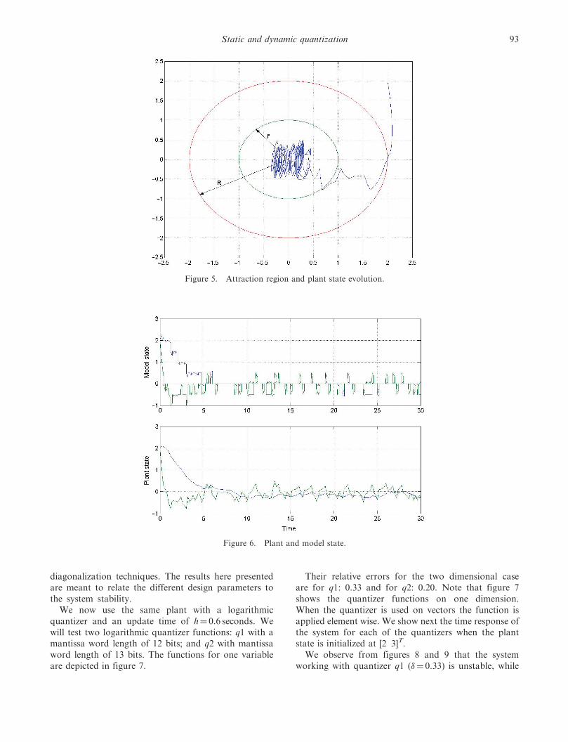
diagonalization techniques. The results here presentedare meant to relate the different design parameters tothe system stability.We now use the same plant with a logarithmic

quantizer and an update time of h¼ 0.6 seconds. Wewill test two logarithmic quantizer functions: q1 with amantissa word length of 12 bits; and q2 with mantissaword length of 13 bits. The functions for one variableare depicted in figure 7.

Their relative errors for the two dimensional caseare for q1: 0.33 and for q2: 0.20. Note that figure 7shows the quantizer functions on one dimension.When the quantizer is used on vectors the function isapplied element wise. We show next the time response ofthe system for each of the quantizers when the plantstate is initialized at [2 3]T.

We observe from figures 8 and 9 that the systemworking with quantizer q1 (�¼ 0.33) is unstable, while

Figure 5. Attraction region and plant state evolution.

Figure 6. Plant and model state.


with q1 (�¼ 0.20) is stable. By using Theorem 3 anda QD¼I we obtain a maximum relative error (18)of 0.1241.

4. Stability of MB-NCS with dynamic quantization

In this section we will consider the case of dynamicquantization, where the quantized region and

quantization error vary at each transmission time. It

has been shown that these type of quantizers can achieve

the smallest bit count per packet while maintaining

stability (Nair and Evans 2000a, b, Ling and

Lemmon 2004). This comes with the price of increased

quantizer complexity. While the static quantizers

did require a relatively small amount of computations,

the dynamic quantizers need to compute new quantiza-

tion regions and detect the plant state presence

Figure 7. Quantizer functions.

Figure 8. Plant and Model state time response for q1.


within each region. Yet dynamic quantizers are anattractive alternative when the number of bits availableper transmission is restricted. Our results extend thosealready available in the literature to the case ofMB-NCS. It will be shown that our results convergeto existing standard literature results when the modeluncertainty is zero.Under the dynamic quantizer scheme, an encoder

measures the state of the plant at each transmission timeand sends a symbol to the decoder collocated with theplant model. To do so, first the encoder and decoderassume that the plant state is contained in a hyper-parallelogram Rk. Next, the encoder uses the plantmodel and plant-model uncertainties to determine theregion where the plant state is at the next transmissiontime. This calculated region will also be a hyper-parallelogram denoted as R�

kþ1. The encoder can alsocalculate R�

kþ1 since its calculation is based on the plantmodel dynamics and known uncertainty bounds.Then, the encoder can divide R�

kþ1 in 2N smaller equalhyper-parallelograms. N is an integer representingthe number of bits used to identify each smallerparallelogram. The encoder then sends an N-bitsymbol representing the smaller parallelogram Rkþ1

within R�kþ1 where the plant state is. The process can

be repeated.We will assume that the plant model matrix A has

distinct real unstable eigenvalues. This assumption canbe relaxed at the expense of more complex notation andproblem geometry. We will also assume that thecompensated model is stable.Previous results (Hespanha et al. 2002, Ling and

Lemmon 2004) consider a similar case but our result

is novel in that it incorporates the plant-modelmismatch within our MB-NCS approach. Ling andLemmon (2004) calculate the minimum bit rate forNCS under network dropouts. Hespanha et al. (2002),consider the case of a NCS that incorporates an exactmodel of the plant. The results in Hespanha et al.(2002) yield the minimum bit rate for stabilizing theNCS under bounded measurement noise and inputdisturbance. A similar method that does not consideruncertainty or model-based techniques is used in Lingand Lemmon (2004) called the uncertain set evolutionmethod. Namely, at transmission time tk, the encoderpartitions the hyper-parallelogram R�

k , containing theplant state x(tk) into 2N smaller hyper-parallelogramsand sends the decoder the symbol identifying thepartition Rk that contains the plant state. Thecontroller then uses the center ck of Rk to updatethe plant model generates the control signal using theplant model until time t�kþ1. At this point, bothencoder and decoder calculate a new hyper-parallelogram R�

kþ1 that should contain the plantstate by evolving or propagating forward the initialregion Rk. The process is then repeated. Stability willbe ensured if the radius and center of the hyper-parallelograms converge to zero with time. We willshow now how the hyper-parallelogram R�

kþ1 isobtained from Rk.

Assume that the plant model matrix A 2 Rnxn hasn distinct unstable eigenvalues l1,l2, . . . , ln with ncorresponding linearly independent normalizedeigenvectors v1, v2, . . . , vn 2 Rn. We will also assumethat at t¼ 0 both encoder and decoder agree upon ahyper-parallelogram R0 containing the initial state

Figure 9. Plant and Model state time response for q2.


of the plant. Denote a hyper-parallelogram as the(nþ 1)-tuple where c is the center of the hyper-parallelogram and �i are its axis. In particular

Rðc, �1, �2, . . . , �nÞ ¼

(x 2 Rn,

Xni¼1

�i�i ¼ x� c,

where �i 2 Rn, �i 2 �1, 1½ �,

and c 2 Rn

):

Let each hyper-parallelogram Rk with center ck bedefined as follows:

RK ¼ Rðck, �k, 1, �k, 2, . . . , �k, nÞ ð22Þ

where

�k, i ¼ bk, ivi and bk, i 2 R:

Therefore it can be easily verified that according to theplant dynamics the region Rk evolves into a hyper-parallelogram R

pkþ1 defined by

Rpkþ1 ¼ R c

pkþ1, �

pkþ1, 1, �

pkþ1, 2, . . . , �

pkþ1, n

� �with �pkþ1, i ¼ eAh�k, i

ð23aÞ

and

cpkþ1 ¼ eAh þ

Z h

0

eAðh�sÞBKeðAþBKÞsds

� �ck: ð23bÞ

Correspondingly, according to the plant modeldynamics the hyper-parallelogram Rk should evolveinto a different hyper-parallelogram Rm

kþ1

Rmkþ1 ¼ R cmkþ1, �

mkþ1, 1, �

mkþ1, 2, . . . , �

mkþ1, n

� �with �mkþ1, i ¼ elih�k, i,

and cmkþ1 ¼ eðAþBKÞhck:

ð24Þ

According to equation (24) the hyper-parallelogramRm

kþ1 has edges that are parallel to those of theoriginal hyper-parallelogram Rk but are longer by afactor of el,h for each corresponding edge. Also thecenter of the parallelogram has shifted. Note thatthe hyper-parallelogram Rm

kþ1doesnot necessarily con-tain the plant state. We will now express R

pkþ1 in terms of

the parameters of Rmkþ1. By replacing h by t and using

Laplace transforms the expressions in (23) can beeasily manipulated

eAh �!L

ðsI� AÞ�1

¼ ðsI� AÞ�1ðsI� AÞðsI� AÞ�1

¼ ðIþ ðsI� AÞ�1 ~AÞðsI� AÞ�1

¼ ðsI� AÞ�1þ ðsI� AÞ�1 ~AðsI� AÞ�1

�!L�1

eAh þ

Z h

0

eAðh�sÞ ~AeAsds

and

eAh þ

Z h

0


�!L

ðsI� AÞ�1þ ðsI� AÞ�1BKðsI� ðAþ BKÞÞ�1

¼ ðsI� AÞ�1ðsI� Aþ ~BKÞðsI� ðAþ BKÞÞ�1

¼ ðsI� ðAþ BKÞÞ�1þ ðsI� AÞ�1

ð ~Aþ ~BKÞ

� ðsI� ðA� BKÞÞ�1

�!L�1

eðAþBKÞh þ

Z h

0

eAðh�sÞð ~Aþ ~BKÞeðAþBKÞsds: ð25Þ

Therefore the parameters of Rpkþ1 can be expressed in

terms of the parameters of Rmkþ1

�pkþ1, i ¼ eAh�k, i¼ eAh þ

Z h

0

eAðh�sÞ ~AeAsds

� ��k, i

¼ eAhbk, ivi þ

Z h

0

eAðh�sÞ ~AeAsds

� ��k, i

¼ elih�k, i þ��ðhÞ�k, i

¼ �mkþ1, i þ��ðhÞ�k, i

cpkþ1 ¼ eAh þ

Z h

0


� �

ck ¼ eðAþBKÞh þ

Z h

0

eAðh�sÞð ~Aþ ~BKÞeðAþBKÞsds

� �ck

¼ eðAþBKÞhck þ

Z h

0

eAðh�sÞð ~Aþ ~BKÞeðAþBKÞsds

� �ck

¼ cmkþ1 þ�cðhÞck: ð26Þ

Note that the matrices �c(h) and ��(h) can be calculatedas follows:

�cðhÞ ¼ ½ I 0 �e

A ~Aþ ~BK

0 AþBK

� �h

� �0

I

� �,

��ðhÞ ¼ ½ I 0 �e

A ~A

0 A

� �h

� �0

I

� �: ð27Þ


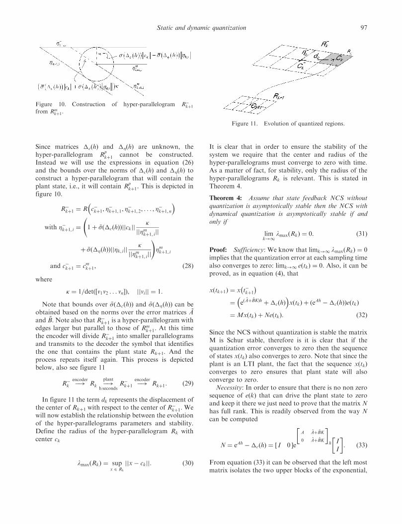
Since matrices �c(h) and ��(h) are unknown, thehyper-parallelogram R

pkþ1 cannot be constructed.

Instead we will use the expressions in equation (26)and the bounds over the norms of �c(h) and ��(h) toconstruct a hyper-parallelogram that will contain theplant state, i.e., it will contain R

pkþ1. This is depicted in

figure 10.

R�kþ1 ¼ R c�kþ1, �

�kþ1, 1, �

�kþ1, 2, . . . , �

�kþ1, n

� �

with ��kþ1, i ¼ 1þ �� cðhÞð Þjjckjj�

jj�mkþ1, ijj

þ ��ð��ðhÞÞjj�k, ijj�

jj�mkþ1, ijj

!�mkþ1, i

and c�kþ1 ¼ cmkþ1, ð28Þ

where

� ¼ 1=det ½v1v2 . . . vn�ð Þ, jjvijj ¼ 1:

Note that bounds over ��ð�cðhÞÞ and ��ð��ðhÞÞ can beobtained based on the norms over the error matrices Aand ~B. Note also that R�

kþ1 is a hyper-parallelogram withedges larger but parallel to those of Rm

kþ1. At this timethe encoder will divide R�

kþ1 into smaller parallelogramsand transmits to the decoder the symbol that identifiesthe one that contains the plant state Rkþ1. And theprocess repeats itself again. This process is depictedbelow, also see figure 11

R�k �!

encoderRk �!

plant

h secondsR�

kþ1 �!encoder

Rkþ1: ð29Þ

In figure 11 the term dk represents the displacement ofthe center of Rkþ1 with respect to the center of R�

kþ1. Wewill now establish the relationship between the evolutionof the hyper-parallelograms parameters and stability.Define the radius of the hyper-parallelogram Rk withcenter ck

lmaxðRkÞ ¼ supx 2 Rk

jjx� ckjj: ð30Þ

It is clear that in order to ensure the stability of thesystem we require that the center and radius of thehyper-parallelograms must converge to zero with time.As a matter of fact, for stability, only the radius of thehyper-parallelograms Rk is relevant. This is stated inTheorem 4.

Theorem 4: Assume that state feedback NCS withoutquantization is asymptotically stable then the NCS withdynamical quantization is asymptotically stable if andonly if

limk!1

lmaxðRkÞ ¼ 0: ð31Þ

Proof: Sufficiency: We know that limk!1 lmaxðRkÞ ¼ 0implies that the quantization error at each sampling timealso converges to zero: limk!1 eðtkÞ ¼ 0. Also, it can beproved, as in equation (4), that

xðtkþ1Þ ¼ x t�kþ1

� �¼ eðAþBKÞh þ�cðhÞ� �

xðtkÞ þ ðeAh ��cðhÞÞeðtkÞ

¼ MxðtkÞ þNeðtkÞ: ð32Þ

Since the NCS without quantization is stable the matrixM is Schur stable, therefore is it is clear that if thequantization error converges to zero then the sequenceof states x(tk) also converges to zero. Note that since theplant is an LTI plant, the fact that the sequence x(tk)converges to zero ensures that plant state will alsoconverge to zero.

Necessity: In order to ensure that there is no non zerosequence of e(k) that can drive the plant state to zeroand keep it there we just need to prove that the matrix Nhas full rank. This is readily observed from the way Ncan be computed

N ¼ eAh ��cðhÞ ¼ ½ I 0 �e

A ~Aþ ~BK

0 AþBK

� �h I

I

� �: ð33Þ

From equation (33) it can be observed that the left mostmatrix isolates the two upper blocks of the exponential,

Figure 10. Construction of hyper-parallelogram R�kþ1

from Rmkþ1.

Figure 11. Evolution of quantized regions.


since the exponential matrix has rank 2n, the isolatedmatrix (of size n�2n) should have rank n. Therefore, anynon zero error vector multiplied by N will yield a nonzero vector. œ

Remarks: Assume that in order to generate thehyper-parallelograms Rkþ1 each edge of the hyper-parallelogram R�

kþ1 is divided in equal Qi parts. Notethat all the Qi must be powers of 2, that is Qi ¼ 2bi wherebi represent the number of bits assigned to each axis. Theresulting bit rate is BitRate ¼

Pni¼1 bi

� �=H. We can now

present a sufficient condition for stability of MB-NCSunder the described dynamic quantization.

Theorem 5: The state feedback MB-NCS using thedynamic quantization described in (29) is globallyasymptotically stable if the following conditions aresatisfied:

(1) The non-quantized MB-NCS is stable.(2) The test matrix T has all its eigenvalues inside the

unit circle.

where

T ¼T11a þ T11b T12

T21 T22

� �

with T11a ¼ diagel1h þ ��ð��ðhÞÞ�

Q1

� �,

�

. . . ,elnh þ ��ð��ðhÞÞ�

Qn

� ��,

T11b ¼

Q1 � 1

Q1

� �. . .

Qn � 1

Qn

� �: :

Q1 � 1

Q1

� �. . .

Qn � 1

Qn

� �266664

377775 ��ð�cðhÞÞ�,

T12 ¼

��ð�cðhÞÞ�

:

��ð�cðhÞÞ�

264

375,

T21‘ ¼Q1 � 1

Q1

� �. . .

Qn � 1

Qn

� �� eðAþBKÞh� �

,

T22 ¼ ��ðeðAþBKÞhÞ ð34Þ

Proof: In order to characterize the evolution of thehyper-parallelograms it is convenient to establishthe relationship between the sizes of edges of R�

kþ1 andthe edges of R�

k

��kþ1, i

�� ¼elih þ ��ð��ðhÞÞ�

Qi

� ��k, i

�� þ ��ð�cðhÞÞ�jjckjj

�elih þ ��ð��ðhÞÞ�

Qi

� ��k, i

�� þ ��ð�cðhÞÞ� c�k

�� þ ��ð�cðhÞÞ�jjdkjj: ð35Þ

Equation (35) is a scalar discrete linear system. It isdependent on c�k

�� . The evolution of ck is given below

c�kþ1 ¼ eðAþBKÞhck ¼ eðAþBKÞhc�k þ eðAþBKÞhdk: ð36Þ

The term kdkk is bounded by

jjdkjj �XNi¼1

��kþ1, i

�� Qi � 1

Qi

� �� : ð37Þ

We will now bound jjc�k jj

c�kþ1

�� eðAþBKÞh� �

c�k��

þ �� eðAþBKÞh� �XN

i¼1

��kþ1, i

�� Qi � 1

Qi

� �� : ð38Þ

From (35), (37) and (38) it is clear that stability isguaranteed if T has its eigenvalues inside the unit circle.

Remarks: Note that if the plant model is exact, ~A ¼ 0and ~B ¼ 0, then �c(h)¼ 0 and ��(h)¼ 0. This impliesthat if ��ðeðAþBKÞhÞ < 1 then stability is guaranteedprovided that maxiðe

lih=QiÞ < 1 which is a well-established result (Nair and Evans 2000a, b). In orderto enforce the condition that ��ðeðAþBKÞhÞ < 1 it isconvenient to apply a similarity transformation thatdiagonalizes Aþ BK. In order to obtain a value of��ðeðAþBKÞhÞ that is close to the magnitude of themaximum eigenvalue of eðAþBKÞh.

Next an example is presented, This example depicts theway a MB-NCS can be designed, namely first a non-quantized MB-NCS is designed and then a suitablequantization scheme is added and tested for stability.

Example 3: Consider the plant described by thefollowing matrices:

A ¼0 1a21 0:5

� �B ¼

0:10:2

� �, ð39Þ

where a11 2 �0:01, 0:01½ � represents the uncertainty inthe A matrix. Let the plant model be the nominal plant,that is

A ¼0 10 0:5

� �B ¼

0:10:2

� �: ð40Þ

A feedback gain K¼ [�3.3333 �8.3333] is selected soto place the eigenvalues of the plant model at (�0.5,�1).An update time of h¼ 1 sec is used. To reduceconservativeness, the following similarity transforma-tion that diagonalizes Aþ BK is applied to the system

xnew ¼ Px, where P ¼1:8856 0:4714

1:3744 1:3744

� �: ð41Þ

Finally, the quantized levels are defined as n1¼ 1 bit andn2¼ 2 bits for the eigenvectors corresponding to the


eigenvalues at �0.5 and �1 respectively. Note the needfor more bits for faster eigenvalues. The bounds for thenorms of the uncertainty matrices are calculated in thetransformed space by searching along the parameter a21;they are as follows:

��ð�cðhÞÞ � 0:1354, ��ð��ðhÞÞ � 0:0961 ð42Þ

The maximum eigenvalue for the test matrix T is 0.9531indicating that the quantized system is stable. Next a

simulation of the system is presented. In this simulationthe parameter a21 is chosen to be 0.0034, the startingregion to have a center [2–3]T, with edges of length 1;the plant state is placed randomly within this region.The plots are in the non-transformed original space(figures 12–14).

In this example we use a simple plant and controllerto show how the design technique is used. Note thatthe complexity of the calculations involved dependson the number of states in the plant. Note that the

Figure 12. Plant state.

Figure 13. Plant model state.


calculations used to determine the stability of aparticular system are performed off-line. In contrastthe calculations used to quantize the plant state vectorare done on-line. For these on-line calculations, theproposed scheme carries a similar computational inten-sity to that of dynamic quantizers without MB-NCSwith the addition of the computations shown in (28) andthe model simulation.

5. Conclusions

Sufficient conditions for the stability of quantizedMB-NCS were presented. These results consider threedifferent types of quantizers. The quantizers studiedrelate to popular data representation models. Inparticular, the uniform quantizer is related to fixed-point number representations, while the logarithmicquantizer is related to the floating-point representation.The results although conservative provide a way torelate the effects of uncertainty, model update times, andnon-networked control robustness to system stability.A third more complex quantizer based on traditionaldynamic quantization was also introduced; the dynamicquantizer uses an integral representation of the data inan adaptive manner. That is, the data transmittedrepresents an area within a region where the state ofthe plant is known to be. The regions evolve accordingto plant model and the uncertainties bound over themodel parameters. It was shown that if the uncertaintiesare eliminated, the minimum data rate needed forstability coincides with the well-known minimaltheoretical rate for stability (Nair and Evans 2000a).

While the computations required to verify stability canbe complex, the calculations performed by the quantizerare similar in nature to those performed by dynamicquantizers that do not consider uncertainty. Animportant feature of the paper is that the results showexplicitly the dependence on several design parameterssuch as modelling error, quantization parameters,measures of robustness.

Acknowledgements

The partial support of the Army Research Office(DAAG19-01-1-0743) and of the National ScienceFoundation (NSF CCR-02-08537, ECS-02-25265) isgratefully acknowledged.

References

B. Bamieh, ‘‘Intersample and finite wordlength effects in sampled-dataproblems’’, in Proc. of the 35th IEEE Conf. on Dec. and Cont., Kobe,Japan, December 1996, pp. 3890–3895.

N. Elia and S. Mitter, ‘‘Stabilization of linear systems with limitedinformation’’, IEEE Trans. Auto. Contr., 46, pp. 1384–1400, 2001.

F. Fagnani and S. Zampieri, ‘‘Stabilizing quantized feedback withminimal information flow: the scalar case’’, 15th InternationalSymposium on Mathematical Theory of Networks and Systems,Notre Dame, IN, USA, 2002.

M. Fu, ‘‘Robust stabilization of linear uncertain systems via quantizedfeedback’’, in Proc. of the 42nd IEEE Conf. on Dec. and Con., Maui,Hawaii USA, December 2003, pp. 199–203.

J. Hespanha, A. Ortega and L. Vasudevan, ‘‘Towards the controlof linear systems: with minimum bit-rate’’, in Proc. of the 15thInt. Symposium on Mathematical Theory of Networks and Sys.,Notre Dame, IN, USA, August 2002.

D. Liberzon and R. Brockett, ‘‘Quantized feedback stabilization oflinear systems’’, IEEE Trans. Auto. Cont., 45, pp. 1279–1289, 2000.

Figure 14. Trajectories for plant state and plant model state showing the evolution of quantized regions.


D. Liberzon, ‘‘Hybrid feedback stabilization of systems with quantizedsignals’’, Automatica, 39, pp. 1543–1554, 2003a.

D. Liberzon, ‘‘On stabilization of linear systems withlimited information’’, IEEE Trans. Auto. Contr., 48, pp. 304–307,2003b.

D. Liberzon, ‘‘Stabilizing a nonlinear system with limited informationfeedback’’, in Proc. of the 42nd IEEE Conf. on Dec. and Cont., Maui,Hawaii USA, December 2003c, pp. 182–186.

Q. Ling and M.D. Lemmon, ‘‘Stability of quantized control systemsunder dynamic bit assignment’’, in Proc. of the 2004 American Cont.Conf., Boston, MA, pp. 4915–4920, 2004.

L.A. Montestruque and P.J. Antsaklis, ‘‘Model-based networkedcontrol systems: necessary and sufficient conditions for stability’’,10th Mediterranean Conf. on Cont. and Automation, Las Vegas, NV,USA, pp. 1620–1625, July 2002a.

L.A. Montestruque and P.J. Antsaklis, ‘‘State and output feedbackcontrol in model-based networked control systems’’, 41st IEEEConf. on Dec. and Cont., December 2002b.

L.A. Montestruque and P.J. Antsaklis, ‘‘On the model-basedcontrol of networked systems’’, Automatica, 39, pp. 1837–1843,2003.

L.A. Montestruque and P.J. Antsaklis, ‘‘Stability of networkedcontrol systems with time-varying transmission times’’, Transact.Auto. Cont., 49, pp. 1562–1572, 2004.

L.A. Montestruque, ‘‘Model-based networked control systems’’. PhDthesis, University of Notre Dame (2004).

G. Nair and R. Evans, ‘‘Stabilization with data-rate-limitedfeedback: tightest attainable bounds’’, Syst. Contr. Lett., 41,pp. 49–56, 2000a.

G. Nair and R. Evans, ‘‘Communication-limited stabilization of linearsystems,’’ Proc. of the Conf. on Dec. and Cont., Sydney, Australia,2000b, pp. 1005–1010.

G. Nair, S. Dey and R. Evans, ‘‘Infimum data rates for stabilisingmarkov jump linear systems’’, in Proc. of the 42nd IEEE Conf. onDec. and Cont, Maui, Hawaii, 2003, pp. 1176–1181.

Networked Control Systems Sessions, in Proceedings of Conference onDecision and Control & Proceedings of American Control Conference,starting in 2003.

J.K. Yook, D.M. Tilbury and N.R. Soparkar, ‘‘Trading computationfor bandwidth: reducing communication in distributed controlSystems using State Estimators’’, IEEE Transact. Contr. Syst.Technol., 10, pp. 503–518, 2002.

G. Walsh, H. Ye and L. Bushnell, ‘‘Stability analysis of networkedcontrol systems’’, in Proc. of American Con. Conf., San Diego, CA,USA, pp. 2876–2880, June 1999.

H. Ye, A.N. Michel and L. Hou, ‘‘Stability analysis of systems withimpulse effects’’, IEEE Transact. Automat. Contr., 43,pp. 1719–1723, 1998.


static and dynamic quantization in model-based networked ...pantsakl/publications/347-ijc07.pdf ·...

Documents