stat 592a spatial statistical methods [email protected] [email protected] nrcse
Post on 22-Dec-2015
221 views
TRANSCRIPT

Course content
1. Kriging 1. Gaussian regression 2. Simple kriging 3. Ordinary and universal kriging 4. Effect of estimated covariance
2. Spatial covariance 1. Isotropic covariance in R2
2. Covariance families 3. Parametric estimation 4. Nonparametric models 5. Covariance on a sphere

3. Nonstationary structures I: deformations 1. Linear deformations 2. Thin-plate splines 3. Classical estimation 4. Bayesian estimation 5. Other deformations 4. Nonstationary structures II: linear combinations
etc. 1. Moving window kriging 2. Integrated white noise 3. Spectral methods 4. Testing for nonstationarity 5. Kernel methods

5. Space-time models1. Separability2. A simple non-separable model3. Stationary space-time processes4. Space-time covariance models5. Testing for separability
6. Assessment and use of deterministic models
1. The kriging approach2. Bayesian hierarchical models3. Bayesian melding4. Data assimilation5. Model approximation
Programs
RgeoR
Fields
S-PlusS+ SpatialStats

Course requirements
Active participationSubmit two lab reports eight homework problems Three homework problems can be
replaced by an approved project
Lab Thursdays 2-4 in B-027 Communications

1. Kriging
NRCSE

Research goals in air quality research
Calculate air pollution fields for health effect studies
Assess deterministic air quality models against data
Interpret and set air quality standards
Improved understanding of complicated systems

The geostatistical model
Gaussian process(s)=EZ(s) Var Z(s) < ∞Z is strictly stationary if
Z is weakly stationary if
Z is isotropic if weakly stationary and
Z(s),s ∈D⊆R2
(Z(s1),...,Z(sk))=d(Z(s1+h),...,Z(sk +h))
μ(s)≡μ Cov(Z(s1),Z(s2))=C(s1−s2)
C(s1−s2)=C0(s1−s2 )
The problem
Given observations at n locationsZ(s1),...,Z(sn)
estimate
Z(s0) (the process at an unobserved place)
(an average of the process)
In the environmental context often time series of observations at the locations.
Z(s)dν(s)A∫or
Some history
Regression (Galton, Bartlett)
Mining engineers (Krige 1951, Matheron, 60s)
Spatial models (Whittle, 1954)
Forestry (Matérn, 1960)
Objective analysis (Grandin, 1961)
More recent work Cressie (1993), Stein (1999)
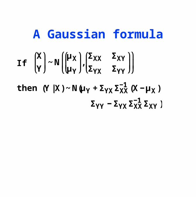
A Gaussian formula
If
then
€
X
Y
⎛
⎝ ⎜
⎞
⎠ ⎟~ N
μX
μY
⎛
⎝ ⎜
⎞
⎠ ⎟,
ΣXX ΣXY
ΣYX ΣYY
⎛
⎝ ⎜
⎞
⎠ ⎟
⎛
⎝ ⎜
⎞
⎠ ⎟
€
(Y |X) ~ N(μY + ΣYXΣXX−1 (X −μX ),
ΣYY − ΣYXΣXX−1 ΣXY )

Simple kriging
Let X = (Z(s1),...,Z(sn))T, Y = Z(s0), so thatX=1n, Y=,
XX=[C(si-sj)], YY=C(0), and
YX=[C(si-s0)].
Then
This is the best unbiased linear predictor when and C are known (simple kriging).
The prediction variance is
p(X) ≡Z(s0 ) = + C(s i −s0 )[ ]T
C(s i −s j )⎡⎣ ⎤⎦−1
X−1n( )
m1 =C(0) − C(s i −s0 )[ ]T
C(s i −s j )⎡⎣ ⎤⎦−1
C(s i −s0 )[ ]
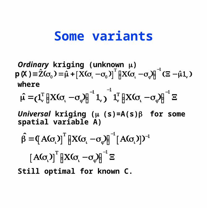
Some variants
Ordinary kriging (unknown )
where
Universal kriging ( (s)=A(s) for some spatial variable A)
Still optimal for known C.
p(X) ≡Z(s0 ) = + C(s i −s0 )[ ]T
C(s i −s j )⎡⎣ ⎤⎦−1
X−1n( )
= 1nT C(s i −s j )⎡⎣ ⎤⎦
−11n( )
−1
1nT C(s i −s j )⎡⎣ ⎤⎦
−1X
=( A(s i )[ ]T
C(s i −s j )⎡⎣ ⎤⎦−1
A(s i )[ ])−1
A(s i )[ ]T
C(s i −s j )⎡⎣ ⎤⎦−1
X
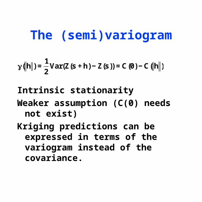
The (semi)variogram
Intrinsic stationarity
Weaker assumption (C(0) needs not exist)
Kriging predictions can be expressed in terms of the variogram instead of the covariance.
γ( h ) =1
2Var(Z(s + h) − Z(s)) = C(0) − C( h )
An example
Ozone data from NE USA (median of daily one hour maxima June–August 1974, ppb)
QuickTime™ and aTIFF (Uncompressed) decompressor
are needed to see this picture.

Fitted variogram
€
γ(t) = σe2 + σs
2 1− e− t
θ ⎛ ⎝ ⎜
⎞ ⎠ ⎟
QuickTime™ and aTIFF (Uncompressed) decompressor
are needed to see this picture.

QuickTime™ and aTIFF (Uncompressed) decompressor
are needed to see this picture.
Kriging surface

QuickTime™ and aTIFF (Uncompressed) decompressor
are needed to see this picture.
Kriging standard error

QuickTime™ and aTIFF (Uncompressed) decompressor
are needed to see this picture.
A better combination
Effect of estimated covariance structure
The usual geostatistical method is to consider the covariance known. When it is estimated• the predictor is not linear• nor is it optimal• the “plug-in” estimate of the variability often has too low mean
Let . Is a good estimate of m2() ?
p2 (X) =p(X; (X))
m1((X))
m2 () =E (p2 (X) −)2 m1()
Some results
1. Under Gaussianity, m2 ≥ m1( with equality iff p2(X)=p(X;) a.s.
2. Under Gaussianity, if is sufficient, and if the covariance is linear in then
3. An unbiased estimator of m2( is
where is an unbiased estimator of m1().
Em1() =m2 () −2(m2 () −m1())
2m−m1()m
Better prediction variance estimator
(Zimmerman and Cressie, 1992)
(Taylor expansion; often approx. unbiased)
A Bayesian prediction analysis takes account of all sources of variability (Le and Zidek, 1992)
Var(Z(s0; )) ≈m1()
+2 tr cov() ⋅cov(∇Z(s0; )⎡⎣
⎤⎦