stat 115: introductory methods for time series analysis

STAT 115: Introductory Methods for

Time Series Analysis and Forecasting

Concepts and Techniques

School of Statistics

University of the Philippines Diliman

1

FORECASTING Forecasting is an activity that

calculates/predicts some future events or

conditions, usually as a result of rational

study or analysis of pertinent data.

Qualitative and Quantitative Forecasting

Qualitative is an intuitive and educated

guess.

Quantitative is based on some

mathematical (deterministic) or statistical

model. 2

Statistical Forecasting Techniques

A Statistical Forecasting Technique

is one that generates forecasts by

extrapolating patterns in historical

data.

Forecasting is linked to the building of

statistical models in the sense that

before one can forecast a variable of

interest, one must build a model for it

and estimate the model’s parameter(s)

using historical data.

3

The estimated model summarizes the

dynamic patterns in the data. It provides a

statistical characterization of the links

between the past and future values.

Statistical Forecasting Techniques

4

Forecasting is an interplay of the data,

statistical techniques and the software

FORECASTING SYSTEM

DATA

QUANTITATIVE

METHODS

SOFTWARE

5

Types of Data

• Cross Section

• Time Series

6

Cross-section data refers to data taken

at one point in time across a group.

Per Capita GRDP, 2001 In Current Prices, Pesos

7

A time series refers to data gathered

sequentially in time.

8

Actual Value = Pattern + Error

When the pattern is clear, this behavior may be used to

explain the behavior of the series & predict future values.

A fundamental assumption of most econometric methods

is that actual value consists of a pattern and an error.

Anatomy of a Model

The pattern and error correspond to a model. A model is

a set of assumptions that summarizes the system

governing a time series.

9

Note:

• Elements entering the model should be assessed using summary statistics.

• Aside from the usual measures of averages, standard deviations, and autocorrelations are important to justify their “predictive” ability in the model.

10

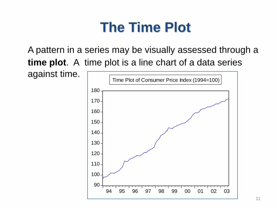
The Time Plot

A pattern in a series may be visually assessed through a

time plot. A time plot is a line chart of a data series

against time.

90

100

110

120

130

140

150

160

170

180

94 95 96 97 98 99 00 01 02 03

Time Plot of Consumer Price Index (1994=100)

11

A time series is usually defined by a model.

Value = function of (Trend, Cycle, Season,

Random Shock)

For example, the gross domestic product in the first

quarter of 2003 is expressed as

GDP 2003.Q1 = f (Trend Component 2003.Q1 ,

Cyclical Component 2003.Q1 ,

First Quarter Seasonal Index,

Random disturbance) 12

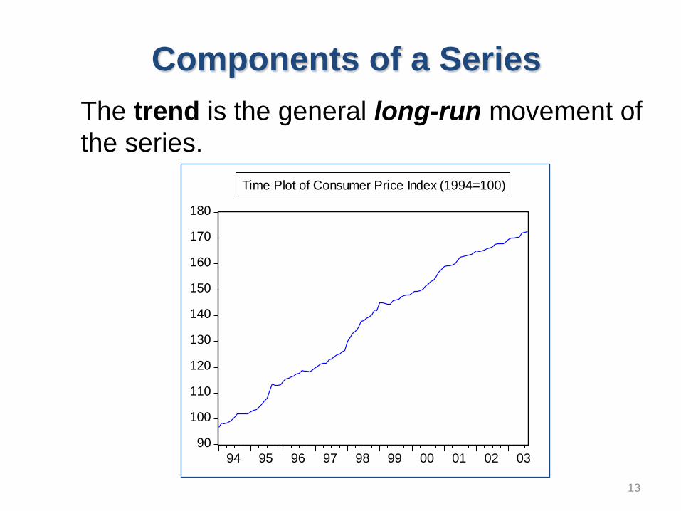
Components of a Series

The trend is the general long-run movement of

the series.

90

100

110

120

130

140

150

160

170

180

94 95 96 97 98 99 00 01 02 03

Time Plot of Consumer Price Index (1994=100)

13

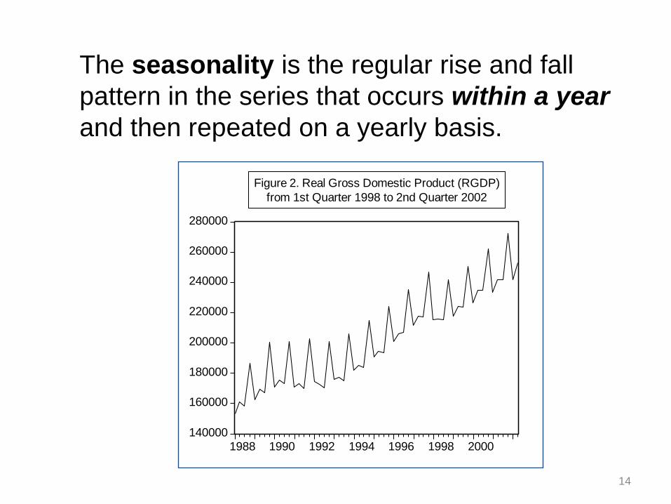
The seasonality is the regular rise and fall

pattern in the series that occurs within a year

and then repeated on a yearly basis.

140000

160000

180000

200000

220000

240000

260000

280000

1988 1990 1992 1994 1996 1998 2000

Figure 2. Real Gross Domestic Product (RGDP)

from 1st Quarter 1998 to 2nd Quarter 2002

14

The cycle is the upward and downward change in

the data pattern that occurs over a longer

duration.

-8

-4

0

4

8

12

1970 1975 1980 1985 1990 1995 2000

Figure 8. Annual GDP Growth Rate from 1970 to 2000

15

The random disturbance is the collection of all

other factors (shocks) affecting the series not

due to trend, cycle or season.

Examples of random

disturbances are day-to-day

natural variation in the

demand that is the result of

a consumer’s specific day-

to-day consumption “mood”.

16

Measuring Forecast Accuracy

T

t t

tt

T

t

tt

Y

YY

T

T

YY

1

1

ˆ100MAPEError Percentage AbsoluteMean

ˆMAD Deviation AbsoluteMean

MSE

T

YYT

t

tt

RMSE Error SquareMean Root

ˆMSE Error SquareMean

1

2

17

An implicit assumption of time series analysis is

that data are collected, observed or recorded at

regular intervals of time. .

Forecasting methods lose some degree of efficiency

when there are gaps in the time series. Thus, there

is a need to estimate missing data.

Estimation of data gaps are usually based on some

trend patterns evident in the series. Most common

trend patterns are linear, exponential and

quadratic.

Addressing Data Gaps

18

2

3

4

5

6

19901991

19921993

19941995

19961997

19981999

2000

A linear trend is exhibited by a line with

minimal variation.

19

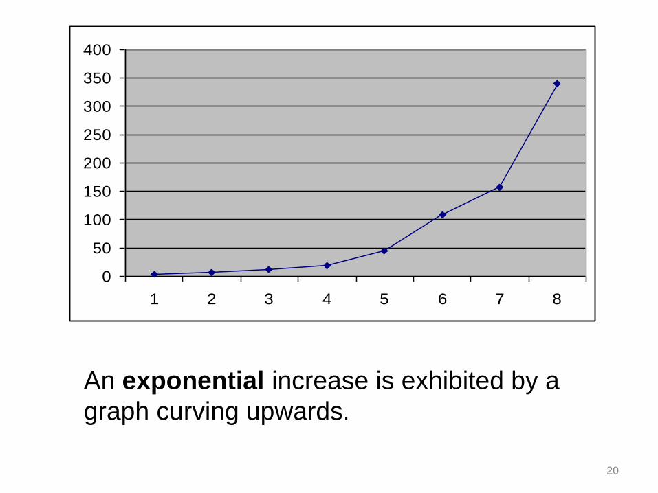
0

50

100

150

200

250

300

350

400

1 2 3 4 5 6 7 8

An exponential increase is exhibited by a

graph curving upwards.

20

15.0

20.0

25.0

30.0

1 2 3 4 5 6 7 8 9 10 11

A quadratic trend is somewhat U-shaped,

concave or convex.

21

Simple Moving Averages

22

Simple Moving Averages

The Simple Moving Average (SMA) is useful in

modeling a series without trend nor seasonality

but only a fluctuation about a common long-term

level.

The method of simple moving averages

assumes that a future value will equal an

average of past values.

23

In general, an N-period moving average denotes

that a new forecast moves one period by adding

the newest actual and dropping the oldest

actual.

For example, a 4-period SMA for May is

SMA4(May) = (Jan+Feb+Mar+Apr)/4.

If the value of the series from Jan to Apr are:

SMA4(May) = (120+124+122+123)/4 = 122.25

24

If the value of the series from Feb to May

are:

Now, a 4-period SMA for June is

SMA4(Jun) = (Feb+Mar+Apr+May)/4.

SMA4(Jun) = (124+122+123+125)/4 = 123.5

25

“H the optimal number of periods in a moving average?”

Here are some considerations The optimal number of period is one that gives minimal forecast error. A long-period SMA yields low forecast error when the series is very random and erratic, i.e., it is not possessing high levels of autocorrelation. A short-period SMA yields low forecast error when the series random yet moves smoothly up and down, i.e., it is highly autocorrelated. The number of period serves as the “length of memory” of the SMA. A four-period SMA “remembers” the past four actuals while an eight-period SMA “recalls” the eight most recent realizations.

26

Disadvantages of the SMA

• SMA’s do not model trend or seasonality.

• All data needed to calculate the average must be

stored and processed.

• It is difficult to determine the optimal number of

periods without the judgment of the researcher

who knows or has institutional memory of the

series.

27

Exponential Smoothing

28

Single Exponential Smoothing

Single exponential smoothing (SES) is

another forecasting tool for data with no trend

or seasonality. SES can be used for short

series.

Why “exponential”?

SES uses forecasting equations based on

past observations that are given

exponentially decaying weights.

29

Why is smoothing important?

Smoothing procedures allow

estimation of future values by

“learning” the historical behavior of

a series. When a forecast is

needed as input in some prediction

equation (like regression models),

smoothing methods “supply” such

forecasts.

30

To forecast using SES, we model

Forecast now = Constant x Past Actual +

(1-constant) x Past Forecast

The forecast equation for a series Yt is

Ft = aY t-1 + (1-a)F t-1

a is called the smoothing constant. It is between

0 and 1. When a great amount of smoothing is desired, a

“small” a must be used. a is chosen such that a chosen measure of

forecast performance (e.g., MAD) is minimized

31

Example: Suppose a company desires to forecast

(monthly) demand of a product using SES with a=0.3.

Last month’s demand was 1,000 and the forecast was

900. Thus, the forecast for this month is

Ft = 0.3(1,000) + (1-0.3)(900) = 930 units

Further, if the actual demand next month is 950 units,

then the forecast two months hence is

Ft+2 = 0.3(950) + (1-0.3)(945) = 946.5 units

Now suppose the actual demand for this month is 980

units, the forecast for next month is

Ft+1 = 0.3(980) + (1-0.3)(930) = 945 units

32

Double Exponential Smoothing

(Brown’s One-Parameter Method)

This is applicable to data with trend but no seasonality.

The forecast equation for Yt+L is

Ft+L = MEANt + TRENDt x L

where MEAN and TREND are the “intercept” and “slope”, respectively, of the forecast equation.

33


Holt-Winters Method

Assumes that a reasonably consistent

seasonal pattern exists, and establishes

this

Combines current level, trend, and

seasonalities to forecast future values

Uses exponential smoothing to estimate

each of these parameters

34


Holt-Winters Method

35


Holt-Winters Method

36


Holt-Winters Method

37


Holt-Winters Method

38


Holt-Winters Method

39


(Holt’s Two-Parameter Method)

This is applicable to data with trend but no seasonality.

This procedure uses two smoothing constants, one each for the mean and the trend; thus allowing for greater flexibility in the values of MEAN and TREND.

40


(Holt’s Two-Parameter Method)


Ft+L = MEANt + TRENDt x L

where MEAN and TREND are the “intercept” and “slope”, respectively, of the forecast equation.

L is the forecast horizon from time t.

41

Triple Exponential Smoothing

(Additive Model)

This method is applicable to data with trend and additive seasonality.


Ft+L = MEANt + TRENDt x L + SEASONt-s+L

where SEASON is the seasonality part and s is the length of seasonality.

42

Triple Exponential Smoothing

(Multiplicative Model)

This is applicable to data with trend and multiplicative seasonality.


Ft+L = (MEANt + TRENDt x L) x SEASONt-s+L

where SEASON is the seasonality index and s is the length of seasonality.

43

“I know of no way of judging the future

but by the past.” Patrick Henry

44

stat 115: introductory methods for time series analysis

Documents