stat 101 introductory statistics - mysmu. · pdf fileintroduction randomness probability...
TRANSCRIPT
Introduction Randomness Probability Probability axioms and rules Probability distributions
STAT 101 Introductory Statistics
August 29, 2017
STAT 101 Class 1 Slide 1
Introduction Randomness Probability Probability axioms and rules Probability distributions
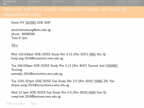
Instructor and TA’s (weekly consultation location and hours, byappointments only)
Denis HY LEUNG SOE 5047
email:[email protected]: 68280396Tues 4-7pm
TA’s
Mon 333-630pm SOE/SOSS Study Rm 3-13 (Rm 3037) ANG Hui [email protected]
Tue 330-630pm SOE/SOSS Study Rm 3-13 (Rm 3037) Samuel Joel [email protected]
Tue 1215-315pm SOE/SOSS Grp Study Rm 2-5 (Rm 2010) YANG Zhi [email protected]
Wed 12-3pm SOE/SOSS Grp Study Rm 2-5 (Rm 2010) KOH Xue [email protected]
STAT 101 Class 1 Slide 2
Introduction Randomness Probability Probability axioms and rules Probability distributions
Essentials
Name card (first few weeks)
Course webpage: http://economics.smu.edu.sg/faculty/
profile/9699/Denis%20LEUNG (NOT eLearn!)
Understanding of basic Calculus and Algebra – Appendix in coursenotes
Readings before each class
Projects vs Homework
Do not disturb others in class
If you missed a class, it is YOUR responsibility to find out what youhave missed from your classmates or course webpage
STAT 101 Class 1 Slide 3

Introduction Randomness Probability Probability axioms and rules Probability distributions
Assessments
Class Participation (10%)
Projects (50%)
– 2 projects with presentation 25% each
– Each project’s grade includes 13% individual assessment(quizzes)
Exam (40%)
– Closed book but one 2-sided A-4 “cheat sheet” is allowed
STAT 101 Class 1 Slide 4
Introduction Randomness Probability Probability axioms and rules Probability distributions
Structure of each class
New materials (< 2.5 hrs)
Break (15 mins)
Any other business (15 mins)
STAT 101 Class 1 Slide 5
Introduction Randomness Probability Probability axioms and rules Probability distributions
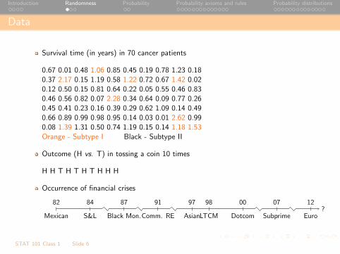
Data
Survival time (in years) in 70 cancer patients
0.67 0.01 0.48 1.06 0.85 0.45 0.19 0.78 1.23 0.180.37 2.17 0.15 1.19 0.58 1.22 0.72 0.67 1.42 0.020.12 0.50 0.15 0.81 0.64 0.22 0.05 0.55 0.46 0.830.46 0.56 0.82 0.07 2.28 0.34 0.64 0.09 0.77 0.260.45 0.41 0.23 0.16 0.39 0.29 0.62 1.09 0.14 0.490.66 0.89 0.99 0.98 0.95 0.14 0.03 0.01 2.62 0.990.08 1.39 1.31 0.50 0.74 1.19 0.15 0.14 1.18 1.53Orange - Subtype I Black - Subtype II
Outcome (H vs. T) in tossing a coin 10 times
H H T H T H T H H H
Occurrence of financial crises
Mexican
82
S&L
84
Black Mon.
87
Comm. RE
91
Asian
97
LTCM
98
Dotcom
00
Subprime
07
Euro
12?
STAT 101 Class 1 Slide 6
Introduction Randomness Probability Probability axioms and rules Probability distributions
Sample vs. Population
(a) Data are a sample from a population that we want to study
e.g., Survival time of 70 patients (sample) out of all cancerpatients (population)
(b) We are interested in some characteristics of the population
e.g., average survival time of patients or percentage of patientswho live beyond 2 years
(c) Due to randomness, we cannot make definitive statements abouta particular unit in the population
e.g., We cannot tell how long the next patient would live
(d) We use the sample of data to help us answer the questions in (b)
STAT 101 Class 1 Slide 7
Introduction Randomness Probability Probability axioms and rules Probability distributions
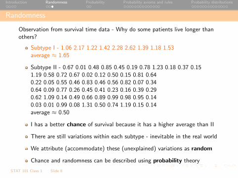
Randomness
Observation from survival time data - Why do some patients live longer thanothers?
Subtype I - 1.06 2.17 1.22 1.42 2.28 2.62 1.39 1.18 1.53average ≈ 1.65
Subtype II - 0.67 0.01 0.48 0.85 0.45 0.19 0.78 1.23 0.18 0.37 0.151.19 0.58 0.72 0.67 0.02 0.12 0.50 0.15 0.81 0.640.22 0.05 0.55 0.46 0.83 0.46 0.56 0.82 0.07 0.340.64 0.09 0.77 0.26 0.45 0.41 0.23 0.16 0.39 0.290.62 1.09 0.14 0.49 0.66 0.89 0.99 0.98 0.95 0.140.03 0.01 0.99 0.08 1.31 0.50 0.74 1.19 0.15 0.14average ≈ 0.50
I has a better chance of survival because it has a higher average than II
There are still variations within each subtype - inevitable in the real world
We attribute (accommodate) these (unexplained) variations as random
Chance and randomness can be described using probability theory
STAT 101 Class 1 Slide 8
Introduction Randomness Probability Probability axioms and rules Probability distributions
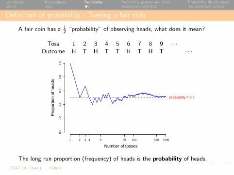
Definition of probability - Tossing a fair coin
A fair coin has a 12 “probability” of observing heads, what does it mean?
Toss 1 2 3 4 5 6 7 8 9 · · ·Outcome H T H T T H T H T · · ·
Pro
port
ion
of h
eads
0.0
0.2
0.4
0.6
0.8
1.0
1 2 3 4 9 50 100 500 1000
probability = 0.5
Number of tosses
The long run proportion (frequency) of heads is the probability of heads.
STAT 101 Class 1 Slide 9

Introduction Randomness Probability Probability axioms and rules Probability distributions
Insight from coin tossing experiment
Probability is the long run frequency of an outcome
Probability cannot predict individual outcomes
However, it can be used to predict long run trends
Probability always lies between 0 and 1, with a value closer to1 meaning a higher frequency of occurrence
Probability is numeric in value so we can use it to:
- compare the relative chance between different outcomes(events)
- carry out calculations
STAT 101 Class 1 Slide 10
Introduction Randomness Probability Probability axioms and rules Probability distributions
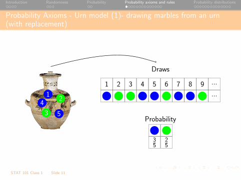
Probability Axioms - Urn model (1)- drawing marbles from an urn(with replacement)
12
4
3 5Probability
35
25
Draws
1 2 3 4 5 6 7 8 9 ...
...
STAT 101 Class 1 Slide 11
Introduction Randomness Probability Probability axioms and rules Probability distributions
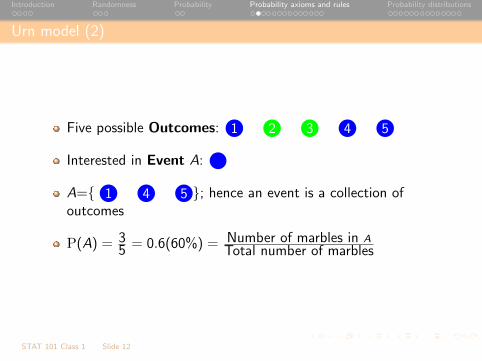
Urn model (2)
Five possible Outcomes: 1 2 43 5
Interested in Event A:
A={ 1 4 5 }; hence an event is a collection ofoutcomes
P(A) = 35 = 0.6(60%) = Number of marbles in A
Total number of marbles
STAT 101 Class 1 Slide 12
Introduction Randomness Probability Probability axioms and rules Probability distributions
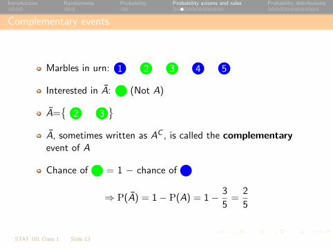
Complementary events
Marbles in urn: 1 2 43 5
Interested in A: (Not A)
A={
2 3}
A, sometimes written as AC , is called the complementaryevent of A
Chance of = 1 − chance of
⇒ P(A) = 1− P(A) = 1− 3
5=
2
5
STAT 101 Class 1 Slide 13
Introduction Randomness Probability Probability axioms and rules Probability distributions
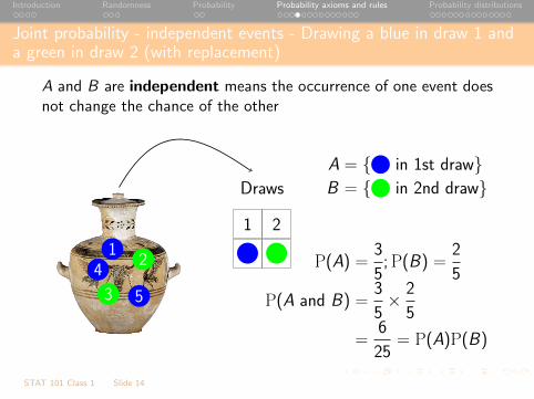
Joint probability - independent events - Drawing a blue in draw 1 anda green in draw 2 (with replacement)
A and B are independent means the occurrence of one event doesnot change the chance of the other
12
4
3 5
Draws
1 2
A = { in 1st draw}B = { in 2nd draw}
P(A) =3
5;P(B) =
2
5
P(A and B) =3
5× 2
5
=6
25= P(A)P(B)
STAT 101 Class 1 Slide 14
Introduction Randomness Probability Probability axioms and rules Probability distributions
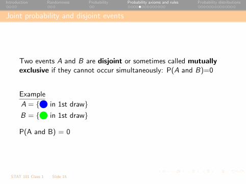
Joint probability and disjoint events
Two events A and B are disjoint or sometimes called mutuallyexclusive if they cannot occur simultaneously: P(A and B)=0
Example
A = { in 1st draw}B = { in 1st draw}
P(A and B) = 0
STAT 101 Class 1 Slide 15
Introduction Randomness Probability Probability axioms and rules Probability distributions
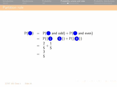
Partition rule
P( ) = P( and odd) + P( and even)
= P({ 1 5 }) + P({ 4 })
=2
5+
1
5
=3
5
STAT 101 Class 1 Slide 16
Introduction Randomness Probability Probability axioms and rules Probability distributions
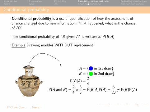
Conditional probability
Conditional probability is a useful quantification of how the assessment ofchance changed due to new information: “If A happened, what is the chanceof B?”
The conditional probability of “B given A” is written as P(B|A)
Example Drawing marbles WITHOUT replacement
?A = { in 1st draw}B = { in 2nd draw}
P(B |A) = 2
4
P(A and B) =2
4× 3
5= P(B |A)P(A) = 6
206= P(B)P(A)
;
STAT 101 Class 1 Slide 17
Introduction Randomness Probability Probability axioms and rules Probability distributions
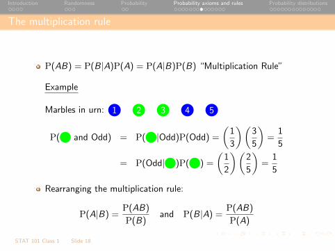
The multiplication rule
P(AB) = P(B|A)P(A) = P(A|B)P(B) “Multiplication Rule”
Example
Marbles in urn: 1 2 43 5
P( and Odd) = P( |Odd)P(Odd) =
(1
3
)(3
5
)=
1
5
= P(Odd| )P( ) =
(1
2
)(2
5
)=
1
5
Rearranging the multiplication rule:
P(A|B) =P(AB)
P(B)and P(B|A) =
P(AB)
P(A)
STAT 101 Class 1 Slide 18
Introduction Randomness Probability Probability axioms and rules Probability distributions
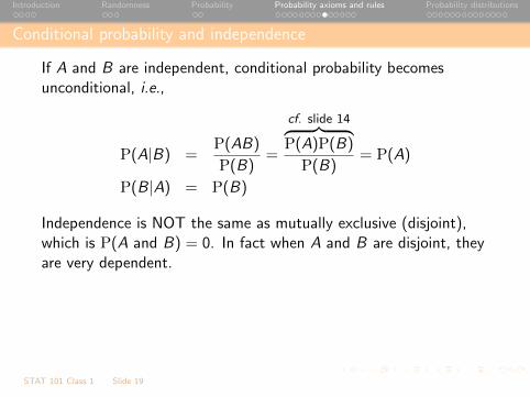
Conditional probability and independence
If A and B are independent, conditional probability becomesunconditional, i.e.,
P(A|B) =P(AB)
P(B)=
cf. slide 14︷ ︸︸ ︷P(A)P(B)
P(B)= P(A)
P(B|A) = P(B)
Independence is NOT the same as mutually exclusive (disjoint),which is P(A and B) = 0. In fact when A and B are disjoint, theyare very dependent.
STAT 101 Class 1 Slide 19
Introduction Randomness Probability Probability axioms and rules Probability distributions
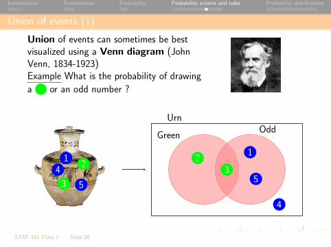
Union of events (1)
Union of events can sometimes be bestvisualized using a Venn diagram (JohnVenn, 1834-1923)Example What is the probability of drawing
a or an odd number ?
12
4
3 5
Urn
GreenOdd
12
4
35
;
STAT 101 Class 1 Slide 20
Introduction Randomness Probability Probability axioms and rules Probability distributions
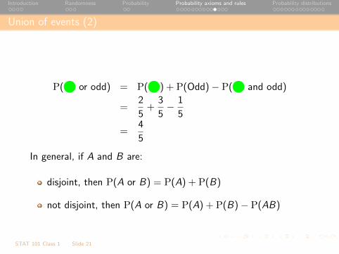
Union of events (2)
P( or odd) = P( ) + P(Odd)− P( and odd)
=2
5+
3
5− 1
5
=4
5
In general, if A and B are:
disjoint, then P(A or B) = P(A) + P(B)
not disjoint, then P(A or B) = P(A) + P(B)− P(AB)
STAT 101 Class 1 Slide 21
Introduction Randomness Probability Probability axioms and rules Probability distributions
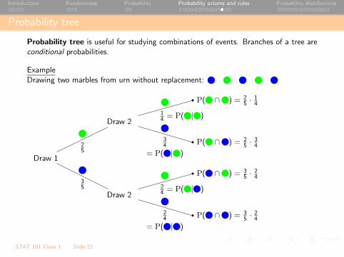
Probability tree
Probability tree is useful for studying combinations of events. Branches of a tree areconditional probabilities.
ExampleDrawing two marbles from urn without replacement:
Draw 1
Draw 2
P( ∩ ) = 35 ·
24
24
= P( | )
P( ∩ ) = 35 ·
24
24 = P( | )
35
Draw 2
P( ∩ ) = 25 ·
34
34
= P( | )
P( ∩ ) = 25 ·
14
14 = P( | )
25
STAT 101 Class 1 Slide 22

Introduction Randomness Probability Probability axioms and rules Probability distributions
Bayes Theorem (Thomas Bayes, 1701-1761)
Trees are useful for visualizing P(B|A) when B follows from A in a natural (time)order. Many problems require P(A|B), Bayes Theorem provides an answer.
ExampleTesting for an infectious disease.
Disease
Test
P(D ∩ T ) = 99100 ·
910
T910
= P(T |D)
P(D ∩ T ) = 99100 ·
110T
110 = P(T |D)
D99100
Test
P(D ∩ T ) = 1100 ·
110
T110
= P(T |D)
P(D ∩ T ) = 1100 ·
910T
910 = P(T |D)
D1
100
What is P(D|T ) or P(D|T )?
STAT 101 Class 1 Slide 23
Introduction Randomness Probability Probability axioms and rules Probability distributions
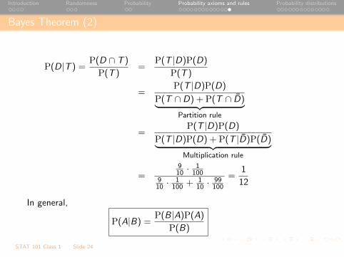
Bayes Theorem (2)
P(D|T ) =P(D ∩ T )
P(T )=
P(T |D)P(D)
P(T )
=P(T |D)P(D)
P(T ∩ D) + P(T ∩ D)︸ ︷︷ ︸Partition rule
=P(T |D)P(D)
P(T |D)P(D) + P(T |D)P(D)︸ ︷︷ ︸Multiplication rule
=910 ·
1100
910 ·
1100 + 1
10 ·99100
=1
12
In general,
P(A|B) =P(B|A)P(A)
P(B)
STAT 101 Class 1 Slide 24
Introduction Randomness Probability Probability axioms and rules Probability distributions
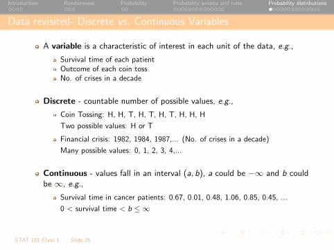
Data revisited- Discrete vs. Continuous Variables
A variable is a characteristic of interest in each unit of the data, e.g.,
Survival time of each patientOutcome of each coin tossNo. of crises in a decade
Discrete - countable number of possible values, e.g.,
Coin Tossing: H, H, T, H, T, H, T, H, H, H
Two possible values: H or T
Financial crisis: 1982, 1984, 1987,... (No. of crises in a decade)
Many possible values: 0, 1, 2, 3, 4,...
Continuous - values fall in an interval (a, b), a could be −∞ and b couldbe ∞, e.g.,
Survival time in cancer patients: 0.67, 0.01, 0.48, 1.06, 0.85, 0.45, ...
0 < survival time < b ≤ ∞
STAT 101 Class 1 Slide 25
Introduction Randomness Probability Probability axioms and rules Probability distributions
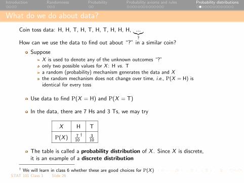
What do we do about data?
Coin toss data: H, H, T, H, T, H, T, H, H, H, ...︸︷︷︸?
How can we use the data to find out about “?” in a similar coin?
Suppose
X is used to denote any of the unknown outcomes “?”only two possible values for X : H vs. Ta random (probability) mechanism generates the data and Xthe random mechanism does not change over time, i.e., P(X = H) isidentical for every toss
Use data to find P(X = H) and P(X = T)
In the data, there are 7 Hs and 3 Ts, we may try
X H T
P(X ) 710
† 310
The table is called a probability distribution of X . Since X is discrete,it is an example of a discrete distribution
† We will learn in class 6 whether these are good choices for P(X )STAT 101 Class 1 Slide 26
Introduction Randomness Probability Probability axioms and rules Probability distributions
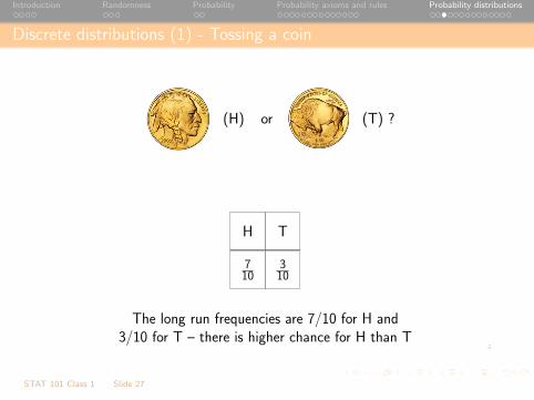
Discrete distributions (1) - Tossing a coin
(H) or (T) ?
H T
710
310
The long run frequencies are 7/10 for H and3/10 for T – there is higher chance for H than T
;
STAT 101 Class 1 Slide 27
Introduction Randomness Probability Probability axioms and rules Probability distributions
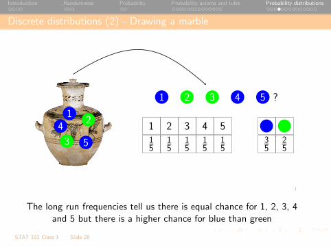
Discrete distributions (2) - Drawing a marble
12
4
3 5
1 2 3 4 5 ?
1 2 3 4 515
15
15
15
15
35
25
;
The long run frequencies tell us there is equal chance for 1, 2, 3, 4and 5 but there is a higher chance for blue than green
STAT 101 Class 1 Slide 28
Introduction Randomness Probability Probability axioms and rules Probability distributions
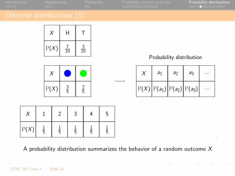
Discrete distributions (3)
X H T
P(X ) 710
310
X 1 2 3 4 5
P(X ) 15
15
15
15
15
X
P(X ) 35
25
X a1 a2 a3 ...
P(X ) P(a1) P(a2) P(a3) ...
Probability distribution
;
A probability distribution summarizes the behavior of a random outcome X
STAT 101 Class 1 Slide 29
Introduction Randomness Probability Probability axioms and rules Probability distributions
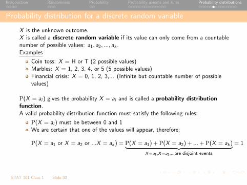
Probability distribution for a discrete random variable
X is the unknown outcome.X is called a discrete random variable if its value can only come from a countablenumber of possible values: a1, a2, ..., ak .Examples
Coin toss: X = H or T (2 possible values)Marbles: X = 1, 2, 3, 4, or 5 (5 possible values)Financial crisis: X = 0, 1, 2, 3,... (Infinite but countable number of possiblevalues)
P(X = ai ) gives the probability X = ai and is called a probability distributionfunction.A valid probability distribution function must satisfy the following rules:
P(X = ai ) must be between 0 and 1We are certain that one of the values will appear, therefore:
P(X = a1 or X = a2 or ...X = ak) = P(X = a1) + P(X = a2) + ...+ P(X = ak)︸ ︷︷ ︸X=a1,X=a2,...are disjoint events
= 1
STAT 101 Class 1 Slide 30
Introduction Randomness Probability Probability axioms and rules Probability distributions
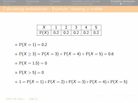
Calculating probabilities - Example: drawing a marble
X 1 2 3 4 5
P(X ) 0.2 0.2 0.2 0.2 0.2
P(X = 1) = 0.2
P(X ≥ 3) = P(X = 3) + P(X = 4) + P(X = 5) = 0.6
P(X = 1.5) = 0
P(X > 5) = 0
1 = P(X = 1)+P(X = 2)+P(X = 3)+P(X = 4)+P(X = 5)
STAT 101 Class 1 Slide 31
Introduction Randomness Probability Probability axioms and rules Probability distributions
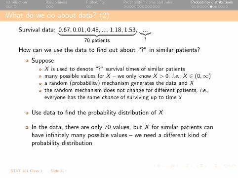
What do we do about data? (2)
Survival data: 0.67, 0.01, 0.48, ..., 1.18, 1.53︸ ︷︷ ︸70 patients
, ...︸︷︷︸?
How can we use the data to find out about “?” in similar patients?
Suppose
X is used to denote “?” survival times of similar patientsmany possible values for X – we only know X > 0, i.e., X ∈ (0,∞)a random (probability) mechanism generates the data and Xthe random mechanism does not change for different patients, i.e.,everyone has the same chance of surviving up to time x
Use data to find the probability distribution of X
In the data, there are only 70 values, but X for similar patients canhave infinitely many possible values – we need a different kind ofprobability distribution
STAT 101 Class 1 Slide 32
Introduction Randomness Probability Probability axioms and rules Probability distributions
Continuous random variable
The survival time (X ) of a cancer patient following diagnosis may beany value in a range (e.g., 0 < X < some positive number).
X is called a continuous random variable if its value falls in a range(a, b) ⊆ (−∞,∞). For a continuous random variable X , P(X = x) forany value x is 0, we can only talk about the probability of X falling ina range
Examples
P(X > 2 years) = Probability of surviving beyond 2 years
P(0 < X ≤ 1 year) = Probability of dying within 1 year
P(X ≤ 2 years|X > 1 year) = Probability of dying within 2years given surviving for 1 year?
STAT 101 Class 1 Slide 33

Introduction Randomness Probability Probability axioms and rules Probability distributions
Probability distribution for a continuous random variable
A continuous random variable, X , is a random variable with outcome that fallswithin a range or interval, (a, b)
Examples
X = survival time of a patient: (a, b) = [0, 150] yearsX = return from an investment of 10000; (a, b) = [−10000,∞) dollarsX = per capita income; (a, b) = [0, 1000000000000] dollars
The probability distribution of X is defined by a (probability) densityfunction (PDF), f (x). There are subtle differences between PDF andprobability:
f (x) ≥ 0 for any value of x in (a, b)f (x) 6= P(X = x) = 0 for any value of xP(r ≤ X ≤ s) = P(r < X < s)︸ ︷︷ ︸
since P(X=r)=P(X=s)=0
probability of X between r and s
P(a ≤ X ≤ b) = 1 since X must fall within (a, b)
The cumulative distribution function (CDF), written as F (x), is defined asP(X ≤ x)
STAT 101 Class 1 Slide 34
Introduction Randomness Probability Probability axioms and rules Probability distributions
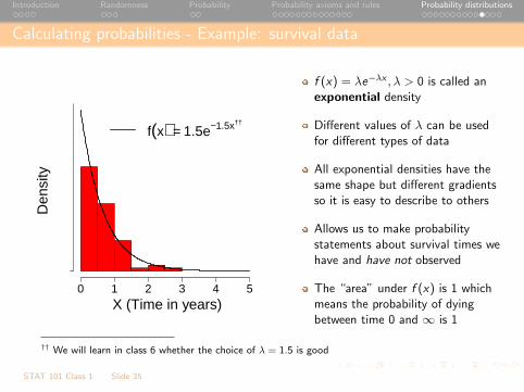
Calculating probabilities - Example: survival data
X (Time in years)
Den
sity
0 1 2 3 4 5
f(x) = 1.5e−1.5x††
f (x) = λe−λx , λ > 0 is called anexponential density
Different values of λ can be usedfor different types of data
All exponential densities have thesame shape but different gradientsso it is easy to describe to others
Allows us to make probabilitystatements about survival times wehave and have not observed
The “area” under f (x) is 1 whichmeans the probability of dyingbetween time 0 and ∞ is 1
†† We will learn in class 6 whether the choice of λ = 1.5 is good
STAT 101 Class 1 Slide 35
Introduction Randomness Probability Probability axioms and rules Probability distributions
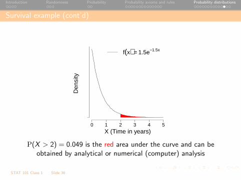
Survival example (cont’d)
X (Time in years)
Den
sity
0 1 2 3 4 5
f(x) = 1.5e−1.5x
P(X > 2)
P(X > 2) = 0.049 is the red area under the curve and can beobtained by analytical or numerical (computer) analysis
STAT 101 Class 1 Slide 36
Introduction Randomness Probability Probability axioms and rules Probability distributions
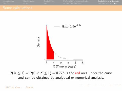
Some calculations
X (Time in years)
Den
sity
0 1 2 3 4 5
f(x) = 1.5e−1.5x
P(X < 1)
P(X ≤ 1) = P(0 < X ≤ 1) = 0.776 is the red area under the curveand can be obtained by analytical or numerical analysis.
STAT 101 Class 1 Slide 37
Introduction Randomness Probability Probability axioms and rules Probability distributions
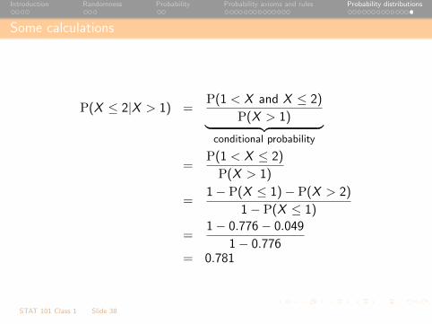
Some calculations
P(X ≤ 2|X > 1) =P(1 < X and X ≤ 2)
P(X > 1)︸ ︷︷ ︸conditional probability
=P(1 < X ≤ 2)
P(X > 1)
=1− P(X ≤ 1)− P(X > 2)
1− P(X ≤ 1)
=1− 0.776− 0.049
1− 0.776= 0.781
STAT 101 Class 1 Slide 38