starting up - eastern illinois universitycfnkv/presentations/spring_conf_02_excel_talk.pdf ·...

Starting up

1. Insert the diskette in the floppy drive

2. Double–click the My Computer icon

3. Double–click the Floppy (A:) icon to open the diskette

4. Double–click on the file Sample to launch Excel

5. Use File, Save As... to make a copy

Andrews & Van Cleave – 45th Annual Conference on the Teaching of Mathematics, March 5, 2002 1

Consult the handout for

terminology

which is unfamiliar to you.


Editing Cells

1. To edit a cell, click in it first

2. Note the selected cell has a darker border

3. Whatever you type in the cell will appear in the

Formula Bar located just above the worksheet

4. Try changing some of the names and scores


Entering New Data

1. Add one or more names and scores across the first empty

row below the other names

2. Insert a new column for another Homework

3. Add a title for the new column

4. Fill in the scores for the new column of Homework


Copying Across a Range

1. Enter 25 beneath Hmwk1 as the perfect score for that

homework

2. Notice the small black square located at the lower–right

corner of the cell. This is a fill handle

3. Click on the fill handle and drag it across the row to

copy the 25 into a range of cells


Selecting Ranges

1. To select a range of cells, click and drag the mouse

across the row, column, or block you want to highlight

2. The sequence is click–drag–release

3. Practice with various ranges


Sorting

1. You must be careful when sorting to keep data with

names!

2. Select the entire range of names and scores, but not

headers or perfect scores

3. Choose Data, then Sort from the menu bar, and sort

by Column A, the names


Formulas & Built-in Formulas1. Formulas are used to calculate such things as sums,

averages, and minimums

2. A formula stars with the = character

3. Some built-in formulas are: SUM AVERAGE COUNT SMALL

4. In the cell below the last Hmwk 1, enter the formula to

find the average of the first homework. Don’t forget to

start with an equals sign.

5. Change some of the scores in that column and watch

the average change


Formatting Cell Contents

1. Select the cell containing the formatted average

2. On the menu bar, click on Format

3. Choose Cells

4. Under Category, select Number

5. When the Decimal places box appears, choose 1

6. Click OK


Copying Formula and Formatting

1. Use the fill handle of the average cell to copy the formula

and formatting across the row to all the other Hmwks

2. Notice how the formula changes, since the range

consisted of relative addresses

3. Notice, too, how the formatting was also copied

4. How is our class doing on their homework?


Student Homework Average1. Next, enter a column for the Hmwk average for each

student in the column to the right of the last Hmwk

2. Add a label at the top of this column

3. Click on the cell in this column in the same row as the

perfect scores

4. Enter a formula to find the average of these homeworks

5. If your formula is correct, the average should be 25

6. When your formula is correct, copy it down the column

to find the average for each student


More Cell Formatting

1. Viewing the average as a percentage of the total

possible...

2. Click on the average cell of the perfect scores

3. Edit the formula to divide the average by 25

4. Format the Cell contents to show a Percentage

5. When the formula and format are both correct, copy

this cell down the column using the fill handle


Dropping Low Scores

1. Move another column to the right—we’re going to add a

column of averages calculated after dropping the lowest

score

2. Add a label to this column

3. Enter your formula in the “perfect” row

4. When it is correct (the average should still be 25), copy

it down the column


Dropping the Two Lowest Scores

1. Now try to figure out the formula for dropping the two

lowest scores, then copy it down the column. You’ll have

to use the SMALL(<range>,2) function to subtract the

second smallest score.

2. Scale this average so that it is out of a possible 15,which is what “perfect” should get


Don’t forget to

SAVE

your worksheet!


Linking Related Worksheets

1. Locate the tabs for the various worksheets in this

workbook at the bottom–left of the Excel window

2. Click on the next worksheet, Quizzes

3. We will link this worksheet with the Homework worksheet

through column A, the student names

4. Click on the cell where the first name should go, and

enter = to begin a formula

5. Click on the Homework tab to move back to that

worksheet


6. Click on the first name there and press Enter. When

you return to the Quizzes worksheet, you should see

the name there

7. Use the fill handle to copy down the links for all the

names


Practice with Averaging

1. Label a column for the quiz averages

2. Enter a formula for finding the average of all but the

worst quiz score, based on a maximum of 20

3. Format the cell

4. Copy it to the entire column


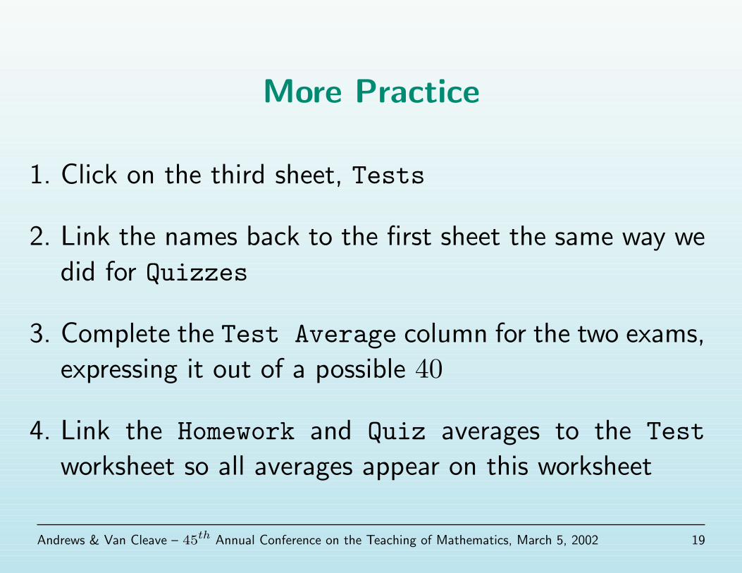
More Practice

1. Click on the third sheet, Tests

2. Link the names back to the first sheet the same way we

did for Quizzes

3. Complete the Test Average column for the two exams,

expressing it out of a possible 40

4. Link the Homework and Quiz averages to the Testworksheet so all averages appear on this worksheet


Grand Finale

1. Compute the course average using a weight of 25 for

the final and summing up all the weighted averages

2. Remember that perfect should get a final weighted

average of 100


THANK YOUfor

Attending!


starting up - eastern illinois universitycfnkv/presentations/spring_conf_02_excel_talk.pdf ·...

Documents