start-up subsidies in east germany: finally, a policy that works?

IZA DP No. 3360

Start-Up Subsidies in East Germany:Finally, a Policy that Works?

Marco Caliendo

DI

SC

US

SI

ON

PA

PE

R S

ER

IE

S

Forschungsinstitutzur Zukunft der ArbeitInstitute for the Studyof Labor

February 2008

Start-Up Subsidies in East Germany:

Finally, a Policy that Works?

Marco Caliendo IZA and IAB

Discussion Paper No. 3360 February 2008

IZA

P.O. Box 7240 53072 Bonn

Germany

Phone: +49-228-3894-0 Fax: +49-228-3894-180

E-mail: [email protected]

Any opinions expressed here are those of the author(s) and not those of IZA. Research published in this series may include views on policy, but the institute itself takes no institutional policy positions. The Institute for the Study of Labor (IZA) in Bonn is a local and virtual international research center and a place of communication between science, politics and business. IZA is an independent nonprofit organization supported by Deutsche Post World Net. The center is associated with the University of Bonn and offers a stimulating research environment through its international network, workshops and conferences, data service, project support, research visits and doctoral program. IZA engages in (i) original and internationally competitive research in all fields of labor economics, (ii) development of policy concepts, and (iii) dissemination of research results and concepts to the interested public. IZA Discussion Papers often represent preliminary work and are circulated to encourage discussion. Citation of such a paper should account for its provisional character. A revised version may be available directly from the author.

mailto:[email protected]

IZA Discussion Paper No. 3360 February 2008

ABSTRACT

Start-Up Subsidies in East Germany: Finally, a Policy that Works?*

The German government has spent between 7bn and 11bn Euro per year on active labor market policies (ALMP) in East Germany in the last decade. The effectiveness of the most important programs (in terms of participants and spending) such as job-creation schemes and vocational training has been evaluated quite thoroughly in recent years. The results are disappointing, indicating that nearly all of these ‘traditional’ programs have to be rated as a failure. In light of these findings, policies to encourage unemployed people to become self-employed gained increasing importance. We present first evidence on the effectiveness of two start-up programs in East Germany. Our findings – even though partly preliminary – are rather promising, showing that these programs increase employment chances and earnings of participants. Hence, start-up subsidies might work even in a labor market with structural problems such as the one in East Germany. JEL Classification: J68, C14, H43, M13 Keywords: start-up subsidies, evaluation, effectiveness, East Germany, self-employment Corresponding author: Marco Caliendo IZA P.O. Box 7240 D-53072 Bonn Germany E-mail: [email protected]

* The author thanks Ulf Rinne for valuable comments. The usual disclaimer applies.

mailto:[email protected]

1 Introduction

Faced with unemployment rates around 20% over the last decade, the German government

spent between 7bn and 11bn Euro per year on active labor market policies (ALMP) in East

Germany to combat this situation. The most important measures (in terms of participants

and spending) during this period have been job-creation schemes and vocational training

programs. The effectiveness of these programs has been evaluated quite thoroughly in

recent years. Based on very informative administrative data and matching techniques,

Biewen, Fitzenberger, Osikominu, and Waller (2007) evaluate the effectiveness of different

training programs, whereas Caliendo, Hujer, and Thomsen (2007) concentrate on job-

creation schemes. The findings are disappointing: Biewen et al. (2007) do not find any

positive effects for short-, medium- or long-term training in East Germany for women and

only little evidence of positive effects for some male subgroups. Caliendo et al. (2007)

show that participating in a job-creation scheme generally lowers the employment chances

of participants; only long-term unemployed women seem to slightly benefit three years

after programs have started. Lechner and Wunsch (2006) compare the relative effects of

different programs (including different types of training, job-creation schemes and shorter

measures) and conclude that all programs do not improve the employment chances or

earnings of participants. Even though they note that the programs might have had other

beneficial effects, judging by the main goal—integration into regular employment—nearly

all of these ‘traditional’ programs have to be rated as a failure.

In light of these disappointing findings the Federal Employment Agency (FEA)

tested a new strategy to combat the unemployment problem by turning unemployment

into self-employment. Whereas in 1994 only 37,000 business start-ups by formerly unem-

ployed individuals where funded, the number was above 350,000 in 2004 (approximately

100,000 in East Germany). This increase was driven, among other things, by a new

program known as the ‘start-up subsidy’ (SUS, Existenzgrundungszuschuss), which was

introduced in 2003 as part of the Hartz reforms and implemented in addition to the already

existing ‘bridging allowance’ (BA, Uberbruckungsgeld). Both programs differ in their de-

sign, the most important difference being in respect of the amount and duration of the

subsidy. While the BA pays recipients the same amount that they would have received

as unemployment benefits for a period of six months (plus a lump sum of roughly 70% to

cover social security contributions), the SUS runs for three years, paying a lump sum of

e600/month for the first year, e360/month for the second, and e240/month for the third.

Later on we will show that this different design also attracted different target groups.

1

Since these programs are usually also associated with the hope for further positive

effects, e.g., through direct job-creation, they could potentially not only decrease East

Germany’s persistently high unemployment rate, but increase its low (self-)employment

rate as well. Looking at the FEA’s spending on ALMP, we clearly see the increasing pri-

ority assigned to these programs within the overall ALMP strategy. Whereas only 1.1% of

ALMP resources were allocated to these measures in 1995, this number was 8.9% in 2004.

Empirical evidence on these programs is scarce in general and non-existent for East Ger-

many. Baumgartner and Caliendo (2007) evaluate the effectiveness of both programs in

West Germany and find considerable positive employment and earnings effects.1 The pa-

pers mentioned above based on administrative data usually exclude start-up subsidies from

the analysis, since the administrative data only includes information on employment which

is subject to social security contributions. Since this is not the case for self-employment,

administrative data does not allow to draw conclusions about employment or earnings

effects for self-employed individuals.

The contribution of this paper is as follows: we evaluate the effectiveness of both

start-up programs in East Germany. Since the major goal of German ALMP is to

avoid future unemployment and integrate unemployed individuals into the primary la-

bor market, we concentrate on the outcome variables ‘not unemployed’ and ‘in paid or

self-employment’. In addition, we analyze the program’s effects on personal income. We

compare the labor market outcomes of the formerly unemployed entrepreneurs with other

unemployed individuals (and not with other business start-ups). This approach is driven

by the consideration that start-up subsidies form one component of ALMP, and their ef-

fectiveness should thus be compared to other ALMP programs. We base our analysis on

a combination of administrative data from the FEA and a follow-up survey, containing

approximately 1,300 participants in both programs who founded a business in the third

quarter of 2003 in East Germany. The interviews took place at the beginning of 2005 and

2006, so that we observe individuals for at least 28 months after programs have started.

While this means we can monitor the employment paths of individuals for at least 22

months after the program has ended for the BA, SUS was still going on at the end of our

observation period. At this stage, participants in SUS were in their third year of partici-

pation and were receiving a reduced transfer payment. Hence, results for this program

are only preliminary and interpretation hinges on this drawback. Additionally, we have a

group of unemployed individuals (approx. 950) who were eligible for either program but

1Caliendo and Steiner (2007) additionally show, that these programs are also monetary efficient (fromthe viewpoint of the Federal Employment Agency).

2

did not choose to participate in the third quarter of 2003. This nonparticipant group will

function as our comparison group.

Given this informative data set, we base our analysis on the conditional independence

assumption and use kernel matching estimators to estimate the treatment effects. To

test the sensitivity of the results with respect to unobserved differences we also use a

conditional difference-in-differences strategy as suggested by Heckman, Ichimura, Smith,

and Todd (1998). The results show that at the end of our observation period both programs

are effective in terms of the above-mentioned outcome variables. Unemployment rates

of participants are lower, and employment rates and personal income are higher when

compared to nonparticipants. Hence, this is first evidence that this relatively new ALMP

instrument might work even in a labor market with structural problems such as the one

in East Germany. Additionally, we present first descriptive evidence on the additional

employment effects trough direct job creation. We find quite significant effects (e.g., 28%

of the males have already at least one employee) for BA, whereas the effects are negligible

for participants in the SUS.

The paper proceeds as follows. Section 2 briefly summarizes some facts about the

East German labor market, focusing on self-employment, unemployment, and active labor

market policies. Section 3 outlines our evaluation approach, while Section 4 describes the

data used for the analysis. In Section 5 we discuss some implementation issues, Section 6

contains the results and, finally, Section 7 concludes.

2 Unemployment, Self-Employment and Start-Up Subsidies

in East Germany

Table 1 contains some summary statistics of the East German labor market. It can be

seen that the self-employment rate has steadily increased from 8% in 1994 to around 11%

in 2004, reaching the same level as West Germany. On the other hand, the unemploy-

ment rate is persistently high, fluctuating around 20% and 22% after 2000. To over-

come this unemployment problem, the German government spends significant amounts

on ALMP (approximately e8 billion in East Germany in 2004) including measures like

vocational training programs, job-creation schemes, employment subsidies, and subsidized

self-employment of formerly unemployed individuals.

Insert Table 1 about here

3

Until 2003 the bridging allowance was the only program providing support to unem-

ployed individuals who wanted to start their own business. Its main goal is to cover basic

costs of living and social security contributions during the initial stage of self-employment.

BA supports the first six months of self-employment by providing the same amount that

the recipient of a BA would have received if he or she had remained unemployed. Since

the unemployment scheme also covers social security contributions (including health insur-

ance, retirement insurance, etc.) a lump sum for social security is granted, equal to 68.5%

of the unemployment support that would have been received in 2003. Unemployed people

are entitled to BA conditional on their business plan being approved externally, usually

by the regional chamber of commerce. Thus, approval of an individual’s application does

not depend on the case manager at the local labor office.

In January 2003, an additional program was introduced to support unemployed

people in starting a new business. This ‘start-up subsidy’ was introduced as part of a large

package of ALMP programs introduced through the ‘Hartz reforms’.2 The main goal of

SUS is to secure the initial phase of self-employment. It focuses on the provision of social

security to the newly self-employed person. The support is a lump sum of e600/month

in the first year. A growth barrier is implemented in SUS such that the support is only

granted if income does not exceed e25,000 per year. The support shrinks to e360/month

in the second year and e240/month in the third. In contrast to the BA, SUS recipients are

obligated to pay into the statutory pension insurance fund and may claim a reduced rate

for statutory health insurance (Koch and Wießner, 2003). When the SUS was introduced

in 2003, applicants did not have to submit business plans for prior approval, but have been

required to do so since November 2004, as was already the case with the BA. See Table

2 for more details on both programs. In this institutional framework, rational program

choice favors a BA if the unemployment benefits are fairly high and/or if the income

generated through the start-up firm is expected to exceed e25,000. Both programs were

replaced in August 2006 by a single new program—the new start-up subsidy program

(Grundungszuschuss)—which will not be analyzed here.3


Hence, for a period of nearly four years, unemployed individuals could choose be-

tween two programs to help them start their own business. Table 1 contains some infor-

2See Caliendo and Steiner (2005) for an overview of the most relevant elements of the ‘Harts reforms’.

3See Caliendo and Kritikos (2007a) for information and a critical discussion of the features of the newprogram.

4

mation on participants and spending in measures promoting self-employment from 1995

to 2004. In 1995, about 2.3% of all unemployed individuals in East Germany partici-

pated in BA, and the FEA spent 1.1% of their total resources for ALMP on BA. Numbers

remained relatively constant until 2003 when the second program was introduced. In

the first year following its introduction, nearly 30,000 individuals made use of the SUS.

Table 1 also shows that the introduction of the SUS did not replace the BA but made

self-employment significantly more attractive for the unemployed (BA entries increased

by roughly 12%).4 In 2004, as much as 6.5% of East Germany’s unemployed participated

in these two programs, absorbing a share of 9% of the total spending on ALMP.

3 Identifying Average Treatment Effects

We base our analysis on the potential outcome framework, also known as the Roy(1951)-

Rubin(1974) model. The two potential outcomes are Y 1 (individual receives treatment,

D = 1) and Y 0 (individual does not receive treatment, D = 0). The actually observed

outcome for any individual i can be written as: Yi = Y 1i ·Di +(1−Di) ·Y 0

i . The treatment

effect for each individual i is then defined as the difference between her potential outcomes:

τi = Y 1i − Y 0

i . Since we can never observe both potential outcomes for the same individual

at the same time, the fundamental evaluation problem arises. We will focus on the most

prominent evaluation parameter, which is the average treatment effect on the treated

(ATT), and is given by:

τATT = E(Y 1 | D = 1) − E(Y 0 | D = 1). (1)

Given equation (1), the problem of selection bias can be straightforwardly seen

since the second term on the right hand side is unobservable. It describes the hypo-

thetical outcome without treatment for those individuals who received treatment. Since

with non-experimental data the condition E(Y 0 | D = 1) = E(Y 0 | D = 0) is usually

not satisfied, estimating ATT by the difference in sub-population means of participants

E(Y 1 | D = 1) and non-participants E(Y 0 | D = 0) will lead to a selection bias. This

bias arises because participants and non-participants are selected groups that would have

different outcomes, even in absence of the program, and might be caused by observ-

able or unobservable factors.5 We will combine two evaluation methods—matching and

difference-in-differences—to cover both possible sources of selection bias.

4Caliendo and Kritikos (2007b) discuss in detail not only the characteristics of the new entrepreneursbut also those of the created businesses.

5See, e.g., Caliendo and Hujer (2006) for further discussion.

5

3.1 Matching under Unconfoundedness

Matching is based on the conditional independence (or unconfoundedness) assumption,

which states that conditional on some covariates W = (X, Z), the potential outcomes

(Y 1, Y 0) are independent of D.6 Since we are interested in ATT only, we only need to

assume that Y 0 is independent of D, because the moments of the distribution of Y 1 for

the treatment group can be directly estimated. That is:

Assumption 1 Unconfoundedness for Comparison Group: Y 0 q D|W,

where q denotes independence. Clearly, this assumption may be a very strong one and has

to be justified on a case-by-case basis, since the researcher needs to observe all variables

that simultaneously influence participation and outcomes. We will do so in Section 5.1.

Additionally, it has to be assumed that:

Assumption 2 Weak Overlap: Pr(D = 1 | W ) < 1,

for all W . This implies that there is a positive probability for all W of not participating,

i.e., that there are no perfect predictors which determine participation. These assumptions

are sufficient for identification of the ATT, which can be written as:

τMATATT = E(Y 1|W,D = 1) − EW [E(Y 0|W,D = 0)|D = 1], (2)

where the first term can be estimated from the treatment group and the second term from

the mean outcomes of the matched comparison group. The outer expectation is taken

over the distribution of W in the treatment group.

As matching on W can become hazardous when W is of high dimension (‘curse

of dimensionality’), Rosenbaum and Rubin (1983) suggest the use of balancing scores

b(W ). These are functions of the relevant observed covariates W such that the conditional

distribution of W given b(W ) is independent of the assignment to treatment, that is,

W q D|b(W ). The propensity score P (W ), i.e., the probability of participating in a

program, is one possible balancing score. For participants and nonparticipants with the

same balancing score, the distributions of the covariates W are the same, i.e., they are

balanced across the groups. Hence, assumption 1 can be re-written as Y 0 qD|P (W ) and

the new overlap condition is given by Pr(D = 1 | P (W )) < 1.

6See Imbens (2004) or Smith and Todd (2005) for recent overviews regarding matching methods.

6

3.2 Combining Matching with Difference-in-Differences

Even though we will argue in Section 5.1 that the CIA is most likely to hold in our

setting, we will test the sensitivity of our results with respect to unobserved heterogene-

ity. The matching estimator described so far assumes that after conditioning on a set

of observable characteristics, (mean) outcomes are independent of program participation.

The conditional DID or DID matching estimator relaxes this assumption and allows for

unobservable but temporally invariant differences in outcomes between participants and

nonparticipants. This is achieved by comparing the conditional before/after outcomes of

participants with those of nonparticipants. DID matching was first suggested by Heckman

et al. (1998). It extends the conventional DID estimator by defining outcomes conditional

on the propensity score and using semiparametric methods to construct the differences.

Therefore, it is superior to DID as it does not impose linear functional form restrictions

in estimating the conditional expectations of the outcome variable, and it re-weights the

observations according to the weighting function of the matching estimator (Smith and

Todd, 2005). If the parameter of interest is ATT, the DID propensity score matching

estimator is based on the following identifying assumption:

E[Y 0t − Y 0

t′ |P (W ), D = 1] = E[Y 0t − Y 0

t′ |P (W ), D = 0], (3)

where (t) is the post-treatment and (t′) the pre-treatment period. It also requires the

common support condition to hold and can be written as:

τCDIDATT = E(Y 1

t − Y 0t′ |P (W ), D = 1) − E(Y 0

t − Y 0t′ |P (W ), D = 0). (4)

4 Data and Some Descriptives

We use a unique data set which combines administrative data from the FEA with survey

data.7 For the administrative part we use data based on the ‘Integrated Labor Market

Biographies’ (ILMB, Integrierte Erwerbs-Biographien) of the FEA, containing relevant

register data from four sources: employment history, unemployment support receipt, par-

ticipation in active labor market measures, and job seeker history. Since the administrative

data are only available with a certain time lag and more importantly, do not provide any

information on the employment status and/or income of self-employed individuals, we en-

7The data was gathered within a research project for the Federal Ministry of Labor (see Forschungsver-bund IAB, DIW, SINUS, GfA, infas, 2006, for details).

7

riched the ILMB data with information from a computer-assisted telephone interview. To

do so, we randomly drew participants from each program who became self-employed in

the third quarter of 2003. Since we wanted to compare them with nonparticipants, we had

to choose a comparison group. Choosing such a group is a heavily discussed topic in the

recent evaluation literature. Although participation in ALMP programs is not mandatory

in Germany, the majority of unemployed persons participate at some point in time. Thus,

comparing participants to individuals who never participate is inadequate, since it can

be assumed that the latter group is particularly selective.8 Sianesi (2004) discusses this

problem for Sweden and argues that those who never participate did not enter a program

because they had already found a job. Additionally, since we did not know the future em-

ployment/participation status of the comparison group before the interviews took place,

we restricted this comparison group to those who were unemployed in the third quarter of

2003, eligible for participation in either of the two programs, but did not join a program

in this quarter. What should be kept in mind is that these comparison group members

might participate in some ALMP program after this quarter.9

To minimise the survey costs we used a crude propensity score matching approach

to select somewhat similar unemployed individuals.10 These individuals were interviewed

twice. The first interview took place in January/February 2005 and the second in Jan-

uary/February 2006. This enables us to observe the labor market activity of individuals

for at least 28 months after programs started. We compiled a sample of 1,297 individuals

who had started a new business out of unemployment. Of these, 647 individuals received

a SUS and 650 received BA. Additionally, a control group of 943 nonparticipants was

assembled.

A full list of the available variables can be found in Table A.1 in the Appendix;

Table 3 contains sample means of the most relevant ones. What should be kept in mind is

the non-random sample of nonparticipants. Since we used a crude matching approach to

make individuals similar, the nonparticipant sample does not represent a random sample

of unemployed individuals. Clearly, this does not affect our estimation and interpretation

8Furthermore, it should be noted that using individuals who are observed to never participate in theprograms as the comparison group may invalidate the conditional independence assumption due to condi-tioning on future outcomes (see discussion in Fredriksson and Johansson, 2007).

9The actual number of nonparticipants who participated in any ALMP program after this quarter israther low. It is approximately 5% after 12, 7% after 18 and around 10% after 24 months.

10The potential comparison group consisted of roughly 330,000 individuals. Control individuals (forthe interview) were chosen to resemble the distribution of some key variables—including gender, region,age, previous unemployment duration, qualification, and nationality—in the population of the treatedindividuals. To do so, we estimated a ‘crude propensity score’ based on these variables and chose for everyparticipant nonparticipants with a similar propensity score as interviewees.

8

strategy but should be kept in mind when interpreting the differences.


A first glance at the number of observations reveals clear gender differences in par-

ticipation in both programs. Whereas the male-female ratio is about 2.2:1 for BA, it is

only 1.3:1 for the SUS. Further differences arise when looking at qualifications. In general

it can be stated that participants in SUS are less qualified (when compared to BA partici-

pants). This is true for the comparison of the participants’ qualifications either by highest

school-leaving degree or the variable ‘job qualifications’, an assessment by the placement

officer in the local labor office. Based on that, it is hardly surprising that participants in

BA programs also have a more favorable labor market history. Not only were they less

frequently found among the long-term unemployed before starting a program they also

had higher and longer claims for unemployment benefits. We will discuss the available

variables in more detail in the next section, where we also discuss the validity of the CIA.

5 Implementing the Estimators

Having discussed our evaluation approach in the previous section, we now present details

on the implementation of the propensity score matching estimator. Caliendo and Kopeinig

(2008) provide an extensive overview of the issues arising when implementing matching

estimators. They point out that a crucial step is to discuss the likely validity of the

underlying CIA. Hence, we deal with this issue in Section 5.1. This will be followed by

the estimation of the propensity score and a discussion of matching details in 5.2.

5.1 Validity of the CIA and Propensity Score Estimation

The CIA is in general a very strong assumption and the applicability of the matching

estimator depends crucially on its plausibility. Blundell, Dearden, and Sianesi (2005)

argue that the plausibility of such an assumption should always be discussed on a case-

by-case basis. Only variables that influence the participation decision and the outcome

variable simultaneously should be included in the matching procedure. Hence, economic

theory, a sound knowledge of previous research and information about the institutional

setting should guide the researcher in specifying the model (see, e.g., Smith and Todd,

2005 or Sianesi, 2004).

9

Both economic theory and previous empirical evaluation studies highlight the im-

portance of socio-demographic and qualificational variables. Regarding the first category

we can use variables such as age, marital status, number of children, nationality (German

or foreigner), and health restrictions. Additionally, we also use information whether indi-

viduals want to work full-time or part-time, and hence we might be able to approximate

the labor market flexibility of these individuals. A second class of variables (qualification

variables) refers to the human capital of the individual, which is also a crucially important

determinant of labor market prospects. The attributes available are school degree, job

qualification, and work experience. Furthermore, previous evaluation studies also point

out that unemployment dynamics and labor market history play a major role in driving

outcomes and program participation. Hence, we use career variables describing the indi-

vidual’s labor market history. The available data in this regard is quite extensive (inter

alia: nearly complete seven-year labor market history; daily earnings from employment;

amount of daily unemployment benefits; duration of last unemployment spell, employ-

ment status before unemployment, previous profession, etc.). Heckman et al. (1998) also

emphasize the importance of drawing treatment and comparison groups from the same

local labor market and giving them the same questionnaire, where the latter is ensured in

our data. To account for the situation on the local labor market, we use a classification of

similar and comparable labor office districts derived by the FEA (see Blien et. al, 2004,

for details). Finally, the institutional structure and the selection process into programs

provide further guidance in selecting the relevant variables. As we have seen from the

discussion in Section 2, the two programs differ, among other things, in the size of the

subsidy. Whereas the SUS is a lump sum, the BA depends on the amount of the unem-

ployment benefits. Hence, we include the daily unemployment transfer payment before

the start of the program as an explanatory variable. In contrast to many other studies, we

are also able to include the remaining duration of unemployment benefits, which probably

plays a determining role in these individuals’ decision.11

Based on this exhaustive data, we argue that the CIA holds in our application. The

set of variables is extensive and covers nearly all variables which have been identified to be

important in previous evaluation studies of labor market policies. However, it should also

be clear that some variables which might influence self-employment dynamics are absent in

our data (see Georgellis, Sessions, and Tsisianis, 2005, for a recent overview). Even though

one might argue that these variables, e.g., intergenerational links, are less important in

11Lechner and Wunsch (2006) evaluate the effectiveness of ALMP (excluding start-up subsidies) in EastGermany using a very similar set of variables.

10

our context (since we compare participants with other unemployed individuals), we test

the sensitivity of the results with respect to time-invariant unobserved differences between

participants and nonparticipants.

5.2 Propensity Score Estimation and Matching Details

Since the choice probabilities are not known a priori, we have to replace them with an

estimate. To do so, we estimate binary conditional probabilities for both programs versus

nonparticipation. Since we estimate the effects separately for men and women, we are left

with four logit estimations. The results can be found in Table A.1 in the Appendix. To

ensure the comparability between the estimates, we choose the same covariates for each

combination and both genders. We do not interpret the results of the propensity score

estimation since we only use this estimation to reduce the dimensionality problem and the

group of participants and nonparticipants are already quite similar due to the construction

of the data.

Insert Figure 1 about here

The distribution of the propensity score is depicted in Figure 1. A visual analysis

already suggests that the overlap between the group of participants and nonparticipants

is sufficient in general. Nevertheless, there are some parts of the distribution (starting

approximately at a propensity score value of 0.7) where the mass of comparison individuals

is quite thin. This is especially true for female participants in BA. However, by using the

usual ‘Minmax’ criterion, where treated individuals are excluded from the sample whose

propensity score lies above the highest propensity score in the comparison group, only 26

individuals are dropped overall.12

Several matching procedures have been suggested in the literature, such as nearest-

neighbor or kernel matching.13 To introduce them, a more general notation is needed: let

I0 and I1 denote the set of indices for nonparticipants and participants. We estimate the

effect of treatment for each treated observation i ∈ I1 in the treatment group by contrasting

her outcome with treatment with a weighted average of control group observations j ∈ I0

12We also test the sensitivity of the results with respect to a stricter imposition of the common supportrequirement, e.g., by dropping 5%(10%) of the individuals where the overlap between participants andnonparticipants is especially low. It turns out that the results are not sensitive.

13See Heckman et al. (1998), Smith and Todd (2005), and Imbens (2004) for overviews.

11

in the following way:

∆MAT =1

N1

∑i∈I1

[Y 1i −

∑j∈I0

ωN0(i, j)Y0j ], (5)

where N0 is the number of observations in the control group I0 and N1 is the number of

observations in the treatment group I1. Matching estimators differ in the weights attached

to the members of the comparison group, where ωN0(i, j) is the weight placed on the j-th

individual from the comparison group in constructing the counterfactual for the i-th indi-

vidual of the treatment group (Heckman et al., 1998). For example, with nearest-neighbor

matching, only the closest neighbor is used to construct the counterfactual outcome, while

kernel matching (KM) is a non-parametric estimator that uses (nearly) all units in the

control group. One major advantage of KM is the lower variance which is achieved because

more information is used for constructing counterfactual outcomes. Since our treatment

and comparison groups are rather small, we will focus on this method in the later empir-

ical application.14 An additional advantage of kernel matching comes from the results of

Heckman, Ichimura, and Todd (1998) who derive the asymptotic distribution of these esti-

mators and show that bootstrapping is valid to draw inference for this matching method.

This allows us to circumvent the issues raised by Abadie and Imbens (2006), pointing out

that bootstrap methods are invalid for NN matching.

Before applying kernel matching, assumptions have to be made regarding the choice

of the kernel function and the bandwidth parameter h. The choice of the kernel appears

to be relatively unimportant in practice (see, e.g., Jones, Marron, and Sheather (1996),

Pagan and Ullah (1999), or DiNardo and Tobias (2001)). What is seen as more important

is the choice of the bandwidth parameter h with the following trade-off arising: high

values of h yield a smoother estimated density function, producing a better fit and a

decreasing variance between the estimated and the true underlying density function. On

the other hand, underlying features may be smoothed away by a large h, leading to a

biased estimate. The choice of h is therefore a compromise between a small variance and

an unbiased estimate of the true density function. Instead of using a ‘rule of thumb’ as

proposed by Silverman (1986), we use ‘leave-one-out’ cross-validation (CV) as suggested in

Black and Smith (2004) and Galdo (2005) to choose h. More details and most importantly,

the chosen bandwidth parameters can be found in Table A.2 in the Appendix. We will

14Additional sensitivity analysis reveals that our results are not sensitive to the matching algorithmchosen. Results are available from the author on request.

12

use these bandwidth parameters for the further empirical analysis.15

To test if the matching procedure is able to balance all the covariates we ran a stan-

dardized difference (SD) test (Rosenbaum and Rubin, 1985). This is a suitable indicator

to assess the distance in marginal distributions of the W -variables. For each covariate W

it is defined as the difference of sample means in the treated and matched control subsam-

ples as a percentage of the square root of the average of sample variances in both groups.

This is a common approach used in many evaluation studies, including those by Lechner

(1999), Sianesi (2004) and Caliendo et al. (2007). Table 4 shows the mean standardized

difference (MSD), i.e., the mean of the SD over all covariates before and after the matching

took place.


It can be seen that the MSD before matching lies between 7.4% for women and 9.2%

for men in SUS and even between 15.1% (men) and 19.4% (women) in BA. The matching

procedure is able to balance the distribution of the covariates very well. The MSD after

matching lies below 5% for all the subgroups. Additionally, Sianesi (2004) suggests re-

estimating the propensity score on the matched sample (i.e., on the participants and

matched nonparticipants) and comparing the pseudo-R2’s before and after matching. After

matching there should be no systematic differences in the distribution of the covariates

between the two groups. Therefore, the pseudo-R2 after matching should be fairly low. As

the results from Table 4 show, this is true for our estimation. The results of the F -tests

point in the same direction, indicating a joint significance of all regressors before but not

after matching. Overall, these are satisfying results and show that the matching procedure

was successful in balancing the covariates between treated individuals and members from

the comparison group. Hence, we move on to the presentation of the results.

6 Results

We discuss the effectiveness of the two programs in relation to nonparticipation based on

three outcome variables: first, we want to know if program participation lowers the risk

of returning to unemployment. To this end, we construct a variable that treats registered

unemployment as a failure and all possible other states as a success (outcome variable

A). Since avoiding unemployment is one of the two major goals of German ALMP, this

15Estimations are done using the PSMATCH2 Stata ado-package by Leuven and Sianesi (2003).

13

allows us to analyze the effectiveness of the programs in reaching this goal. A second aim

is integration into regular, stable employment. Hence, we construct a second outcome

variable which treats ongoing self-employment and regular paid employment as a success

(outcome variable B). Finally, we also assess the effects of the programs on the personal

income of participants. We start the discussion with the employment effects over time,

before we present cumulated effects and income effects. For the latter two, we also present

conditional difference-in-differences results to test the sensitivity.

Effects on the Employment Status over Time: Figure 2 presents the treatment

effects over time, where the upper panel relates to outcome variable A (not unemployed)

and the lower part to outcome variable B (self-employed or in regular employment). Effects

for men (women) are depicted on the left (right) side of each row. Rows 1 and 3 show the

effects of participating in SUS vs. nonparticipation, whereas rows 2 and 4 show the effects

of BA.

Effects start in the first month after the treatment has begun. Before starting

the interpretation, one has to note the following: a look at both figures shows a strong

positive effect at the beginning of our observation period. This can be seen as a ‘positive

locking-in effect’. Whereas a locking-in effect usually corresponds to a negative effect

during participation in a program—for example, vocational training—the findings for our

programs are the opposite. Both participants and nonparticipants are unemployed in

the month before the treatment starts, then participants join the program and change

immediately to the ‘hoped-for’ state. That is, they leave unemployment and become self-

employed, which is viewed as a success for both outcome variables. Hence, one should

not overemphasize this large effect at the start of the self-employment spell. BA runs

out after six months, and a reasonable interpretation should start there. Clearly, for the

three-year-long SUS, the problem is that participants may receive aid during the complete

observation period, interfering with interpretation. However, after 12 months, the transfer

payment is reduced from e600 to e360 and after 24 months it is further reduced to e240.

Since this reduced payment is hardly sufficient to cover social security contributions, it

gives us an initial idea of the success of the newly self-employed.

Insert Figure 2 about here

Let us start the discussion with outcome variable A. In the first months after treat-

ment starts, we have very high positive effects for both programs, lying well above 60

percentage points, irrespective of program and gender. This means, for example, that

14

the unemployment probability of participants in SUS or BA is about 60 percentage points

lower than the unemployment probability of nonparticipants. Clearly, results at that point

have to be interpreted with care since both programs are still going on. The effects show

a negative time trend, where the paths of the programs are very similar up to month six.

After that, the transfer payment for participants in BA terminates and the effects plunge.

The downward trend continues but the rate of decrease is much lower. At the end of our

observation period, that is, 28 months after programs have started, we get an effect of

approximately 28 percentage points for male and 23 percentage points for female partici-

pants in BA. If we look at the effect of SUS versus nonparticipation, the downward trend

is much smoother, spiking somewhat in month 12, but decreasing relatively constantly to

an effect of 34 percentage points for males and 44 percentage points for females in month

28.16 A similar pattern—but on a higher level—can be found for outcome variable B (see

lower part of Figure 2). This is a strong indication that both programs are not only effec-

tive in avoiding unemployment but that they also give individuals much higher chances of

remaining employed (either in paid or self-employment). The differences in both outcome

variables can be explained by the fact that outcome variable A only treats registered un-

employment as a failure. When individuals retreat from the labor market—and this might

be especially relevant for women—they are not counted as a failure. Hence, the second

outcome variable, only treating individuals as a success if they are in employment, has

more explanatory power.

Cumulated Effects: Table 5 contains the cumulative effects over time, i.e., the cumu-

lative monthly effects over the observation period. For the outcome variable ‘not unem-

ployed’ this shows the difference in months spent in unemployment between participants

and nonparticipants. It can be seen that male participants in SUS spend roughly 13.9

months less in unemployment than nonparticipants. For female participants in SUS the

effect is approximately 16.4 months. The cumulative effect for participants in BA is slightly

lower, at 11.6 months for men and 11.1 months for women. We have already discussed

that the effects for the outcome variable ‘self-employment or paid employment’ are even

higher, which is also reflected by the cumulative effects of around 15.5 (19.0) months for

men (women) in SUS and 13.2 (13.8) months for men (women) in BA.

16The dip in the effects, especially for men, between months 16 and 20 is caused by a change in theinterview information. Individuals were interviewed twice, in 2005 and 2006. Months 16 to 20 mightinvolve a time overlap between the first and second interview and might be prone to recall errors. Hence,information for these months should be interpreted with care. For the overall interpretation, especiallywhen moving towards the end of the observation period, this should not pose any problems.

15


As outlined in Section 3.2, we also tested the sensitivity of our results with respect

to time-invariant unobserved heterogeneity by using a conditional difference-in-differences

approach. Before using such an approach, one has to determine the reference level for

the before/after difference. We choose three different time periods for the comparison.

In the first approach we use the time period from 1997 to 2002, that is, the six-year

employment history before entering the program. For the first outcome variable, we sum

the months not spent in unemployment, whereas for the second, we sum the months spent

in paid employment. Additionally, we restrict the reference period to the latest three years

(2000-2002) as well as the earliest three years (1997-1999).

Looking at the table, we see that the results are remarkably stable. For example, the

effect on outcome variable B for men in SUS was 13.9 months with the matching approach

and varies between 13.9 and 14.1 months with the CDID approaches. For the other groups

the variation is similar and shows that additionally controlling for possible unobserved

differences between participants and nonparticipants did not add much information for

our estimates. This can be seen as evidence of the validity of the CIA in our context.

Even when looking at outcome variable B, the variation is still negligible.

Effects on Personal Income: After having established that participants in both pro-

grams are more likely to be employed and less likely to be unemployed than nonpar-

ticipants, we now investigate whether participants also earn more money. We use two

income-related outcome variables: the more relevant one is monthly income from self-

employment or paid employment (labor income). However, since it is often argued that

differences between (low) labor income and unemployment benefits are especially low in

Germany, we will also look at the total personal income of individuals, that is, including

support such as unemployment benefits.


Table 6 contains the results for both outcome variables. Once again, we first present

the results from matching estimates before presenting CDID results.17 It is quite striking

that all participants have higher incomes than nonparticipants for both possible outcome

variables. However, for females some of the differences are not significant. The upper half

17For the DID procedure we use three reference levels: 1) The monthly unemployment benefits beforethe program started, 2) the average monthly income in 2002 and 3) the average monthly income fromregular employment in 2002.

16

of Table 6 reveals that male participants in SUS earn around e600 per month more than

their counterparts in the comparison group. Once again, the CDID does not add much

information to the matching estimates since all estimates range between e620 and e690.

For female participants, the effect is much lower (around e320) but still significant. The

effects for the participants in BA is even higher. Male participants earn about e820 more

per month. For females, the effect, with e290, is comparable to the effect for the SUS

participants. Hence, we can conclude that participating in either of the two programs has

helped individuals to earn more money at the end of our observation period. For males

this finding remains unaffected even if we use the total personal income of individuals as

an outcome variable, where we additionally take unemployment benefits and other public

transfers into account. For females, however, looking at this outcome variable reveals

that there are no significant differences in the total income of female participants and

nonparticipants.

Direct Employment Effects - Descriptive Evidence: Policy makers usually hope

for a second positive effect when subsidizing start-ups: additional employment effects

through direct job-creation. Even though the effects of these policies on (overall) employ-

ment cannot be judged by microeconometric analysis (since macroeconomic effects would

have to be taken into account), we want to present some descriptive evidence on the extent

of these potential effects.


Table 7 contains information on the share of start-ups which have employees 28

months after the programs started as well as the number of employees. Two findings are

striking: first, participants in BA are at this point in time more likely to have employees.

Second, it is rather unlikely that the businesses created with the start-up subsidy will

generate considerable additional employment in the future. To be more specific: 28%

(22%) of the male (female) participants in BA already have at least one employee at the

time of the second interview, whereas this is true for only 8–9% of the participants in

SUS. Male participants in BA not only have the most employees (around 4) but also the

highest share of regular employees (around 56%). Clearly, these numbers do not allow

to draw conclusions about the relative effectiveness of the two start-up subsidies since

the businesses started differ in a variety of aspects (e.g., start-up capital, industry, etc.).

Looking at the lower part of Table 7 shows that participants who have no employees yet

are also reluctant concerning the prospect of employing someone in the future. This is

17

especially the case for the participants in SUS. Being asked whether they would like to

employ further persons in the future, 50% (37%) of the females (males) answered ‘No, by

no means’ and 34% (36%) ‘Rather no’. Hence, it is rather unlikely that these businesses

will create significant additional employment in the future.

7 Conclusion

The aim of this paper has been to evaluate two active labor market programs in East

Germany for which no empirical evidence on their effectiveness had been gathered so far.

In light of the rather disappointing performance of other programs in East Germany—

including training programs, wage subsidies and job-creation schemes—our findings are

rather promising, showing that these programs designed to encourage unemployed people

to become self-employed might have the potential not only to combat East Germany’s

problem of persistently high unemployment, but also to increase its low (self-)employment

rate.

Our analysis is based on a dataset that combines administrative with survey data

and allows us to follow the employment paths of individuals for a period of 28 months

after the programs have started. For the first program under consideration—the bridging

allowance—we observed participants for 22 months after the program ended. However,

participants in the second program—the start-up subsidy—are in their third year of par-

ticipation at the end of our observation period and mostly still receive further support

(although at a reduced rate). Therefore, the results for SUS have to be treated as pre-

liminary. Given the relatively stable participant structure in the BA program since the

introduction of the SUS, one can argue that the SUS attracts a different ‘clientele’ for

self-employment. In general it can be stated that participants in SUS are less qualified

(when compared to BA participants) and that this program is more frequently used by

women.

We have evaluated the effectiveness of both programs relative to nonparticipa-

tion. To this end we used a kernel matching estimator and a conditional difference-and-

differences estimator. Three outcome variables were of major interest. The first was ‘not

unemployed’, corresponding to one of the main aims of the FEA. The second one combines

the two possible labor market states ‘in self-employment’ and ‘in paid employment’ into

one success criterion. The results indicate that both programs are successful: at the end of

our observation period, the unemployment rate of participants in BA was approximately

25 percentage points lower than that of nonparticipants, and for participants in SUS it

18

was around 34 percentage points lower for men and as much as 44 percentage points lower

for women. Additionally, both the probability of being in self-employment and/or paid

employment and the personal income are significantly higher for participants, even though

the income effects for women are not always significant.

This is one of the first studies that allows inferences to be drawn about the effec-

tiveness of start-up programs in East Germany. Most previous studies on the effectiveness

of ALMP in the eastern part of Germany neglected these programs since the used admin-

istrative data does not contain information on employment (or earnings) of self-employed

individuals. In contrast to the other programs that have been evaluated recently (includ-

ing job-creation schemes and vocational training programs), we find considerable positive

effects for start-up subsidies. Hence, programs aimed at turning the unemployed into

entrepreneurs may be a promising strategy in East Germany.

To allow more precise policy recommendations, further research is needed. First

of all, the observation period for the start-up subsidy is still quite short and should be

extended. This will be especially important to judge the income effects for women, which

are already partly not significant at the moment. Second, the relative effects of both

programs should be estimated, which would allow their respective designs to be judged as

well as their suitability for different target groups. Additionally, it would be of interest to

look at the development of the start-ups in terms of turnover and number of jobs directly

created. Such an investigation would also enable an extensive cost-benefit analysis taking

direct (and indirect) costs and benefits into account.

19

References

Abadie, A. and G. Imbens (2006). On the Failure of the Bootstrap for Matching Estima-tors. Working Paper, Harvard University.

Baumgartner, H. and M. Caliendo (2007). Turning Unemployment into Self-Employment:Effectiveness of Two Start-Up Programmes. IZA Discussion Paper No. 2660, forthcom-ing in: Oxford Bulletin of Economics and Statistics.

Biewen, M., B. Fitzenberger, A. Osikominu, and M. Waller (2007). Which Programfor Whom? Evidence on the Comparative Effectiveness of Public Sponsored TrainingPrograms in Germany. Discussion Paper 2885, IZA.

Black, D. and J. Smith (2004). How Robust is the Evidence on the Effects of the CollegeQuality? Evidence from Matching. Journal of Econometrics 121 (1), 99–124.

Blien, U., F. Hirschenauer, M. Arendt, H. J. Braun, D.-M. Gunst, S. Kilcioglu, H. Klein-schmidt, M. Musati, H. Roß, D. Vollkommer, and J. Wein (2004). Typisierung vonBezirken der Agenturen der Arbeit. Zeitschrift fur Arbeitsmarktforschung 37 (2), 146–175.

Blundell, R., L. Dearden, and B. Sianesi (2005). Evaluating the Impact of Education onEarnings in the UK: Models, Methods and Results from the NCDS. Journal of theRoyal Statistical Society, Series A 168 (3), 473–512.

Bundesagentur fur Arbeit (various issues). Arbeitsmarkt. Nurnberg.

Caliendo, M. and R. Hujer (2006). The Microeconometric Estimation of Treatment Effects- An Overview. Allgemeines Statistisches Archiv 90 (1), 197–212.

Caliendo, M., R. Hujer, and S. Thomsen (2007). The Employment Effects of Job CreationSchemes in Germany - A Microeconometric Evaluation. IZA Discussion Paper No.1512, forthcoming in: Advances in Econometrics, 21 .

Caliendo, M. and S. Kopeinig (2008). Some Practical Guidance for the Implementationof Propensity Score Matching. Journal of Economic Surveys 22 (1), 31–72.

Caliendo, M. and A. Kritikos (2007a). Die reformierte Existenzgrundungsforderung furArbeitslose: Chancen und Risiken. Discussion Paper 3114, IZA, Bonn.

Caliendo, M. and A. Kritikos (2007b). Start-Ups by the Unemployed: Characteristics,Survival and Direct Employment Effects. Discussion Paper 3220, IZA, Bonn.

Caliendo, M. and V. Steiner (2005). Aktive Arbeitsmarktpolitik in Deutschland: Bestand-saufnahme und Bewertung der mikrookonomischen Evaluationsergebnisse. Zeitschriftfur Arbeitsmarktforschung / Journal for Labour Market Research 38 (2-3), 396–418.

Caliendo, M. and V. Steiner (2007). The Monetary Efficiency of Start-Up Subsidies inGermany. Mimeo, Bonn/Berlin.

DiNardo, J. and J. Tobias (2001). Nonparametric Density and Regression Estimation.Journal of Economic Perspectives 15 (4), 11–28.

Forschungsverbund IAB, DIW, SINUS, GfA, infas (2006). Evaluation der Maßnahmenzur Umsetzung der Vorschlage der Hartz-Kommission: Wirksamkeit der Instrumente:Existenzgrundungen (Modul 1e). Berlin: Federal Ministry of Labor.

Fredriksson, P. and P. Johansson (2007). Dynamic Treatment Assignment - The Conse-quences for Evaluations Using Observational Data. Journal of Business and EconomicStatistics.

20

Galdo, J. (2005). Bandwidth Selection and the Estimation of Treatment Effects withNon-Experimental Data. Working paper, Syracuse University.

Georgellis, Y., J. Sessions, and N. Tsisianis (2005). Self-Employment Longitudinal Dy-namics: A Review of the Literature. Discussion Paper, Brunel University.

Heckman, J., H. Ichimura, J. Smith, and P. Todd (1998). Characterizing Selection BiasUsing Experimental Data. Econometrica 66 (5), 1017–1098.

Heckman, J., H. Ichimura, and P. Todd (1998). Matching as an Econometric EvaluationEstimator. Review of Economic Studies 65 (2), 261–294.

Imbens, G. (2004). Nonparametric Estimation of Average Treatment Effects under Exo-geneity: A Review. The Review of Economics and Statistics 86 (1), 4–29.

Jones, M., S. Marron, and S. Sheather (1996). A Brief Survey of Bandwidth Selection forDensity Estimation. Journal of the American Statistical Association 91 (433), 401–407.

Koch, S. and F. Wießner (2003). Wer die Wahl hat, hat die Qual. IAB Kurzbericht (2).

Lechner, M. (1999). Earnings and Employment Effects of Continuous Off-the-Job Trainingin East Germany After Unification. Journal of Business Economic Statistics 17 (1), 74–90.

Lechner, M. and C. Wunsch (2006). Active Labour Market Policy in East Germany:Waiting for the Economy to Take Off. Discusssion Paper No. 2363, IZA, Bonn.

Leuven, E. and B. Sianesi (2003). PSMATCH2: Stata Module to Perform Full Mahalanobisand Propensity Score Matching, Common Support Graphing, and Covariate ImbalanceTesting. Software, http://ideas.repec.org/c/boc/bocode/s432001.html.

Pagan, A. and A. Ullah (1999). Nonparametric Econometrics. Cambridge: CambridgeUniversity Press.

Rosenbaum, P. and D. Rubin (1983). The Central Role of the Propensity Score in Obser-vational Studies for Causal Effects. Biometrika 70 (1), 41–50.

Rosenbaum, P. and D. Rubin (1985). Constructing a Control Group Using MultivariateMatched Sampling Methods that Incorporate the Propensity Score. The AmericanStatistican 39 (1), 33–38.

Roy, A. (1951). Some Thoughts on the Distribution of Earnings. Oxford Economic Pa-pers 3 (2), 135–145.

Rubin, D. (1974). Estimating Causal Effects to Treatments in Randomised and Nonran-domised Studies. Journal of Educational Psychology 66, 688–701.

Sianesi, B. (2004). An Evaluation of the Swedish System of Active Labour Market Pro-grammes in the 1990s. The Review of Economics and Statistics 86 (1), 133–155.

Silverman, B. (1986). Density Estimation for Statistics and Data Analysis. London:Chapman & Hall.

Smith, J. and P. Todd (2005). Does Matching Overcome LaLonde’s Critique of Nonex-perimental Estimators? Journal of Econometrics 125 (1-2), 305–353.

21

Tables and Figures

Table 1: Self-employment, Unemployment and Start-Up Subsidies in East Germany, 1994-2004

1994 1995 1998 1999 2000 2001 2002 2003 2004

Self-employeda (in %) 8.0 8.1 8.8 8.9 9.2 9.6 9.9 10.4 11.0Unemployeda (in %) 15.1 13.6 20.4 19.9 20.2 20.8 21.5 22.6 22.2

ALMP participants (Entries in thousand)Vocational Training – – 235.9 183.3 213.7 188.4 198.2 92.3 61.1Job-Creation Schemes – – 271.8 210.5 181.4 130.1 121.4 109.4 112.9Bridging Allowance 15.1 23.9 31.6 32.2 33.7 34.4 38.2 43.4 46.1Start-Up Subsidy – – – – – – – 29.2 57.5Sup. Self-Employment (total) 15.1 23.9 31.6 32.2 33.7 34.4 38.2 72.6 103.6Sup. Self-Employmentb (total in %) 1.3 2.3 2.1 2.2 2.2 2.2 2.5 4.5 6.5

ALMP expenditure (in bn Euro)ALMP - Total -.- 10.19 10.28 11.41 9.77 10.12 10.25 8.92 7.63Vocational Training – – 2.79 2.78 2.75 2.79 2.88 1.97 1.28Job-Creation Schemes – – 2.79 2.89 2.67 2.11 1.78 1.31 0.96Bridging Allowancec 0.03 0.11 0.16 0.23 0.22 0.23 0.27 0.32 0.37Start-Up Subsidy – – – – – – – 0.09 0.31Sup. Self-Employment (total) 0.03 0.11 0.16 0.23 0.22 0.23 0.27 0.41 0.68Sup. Self-Employment (total in %) -.- 1.1 1.6 2.0 2.2 2.3 2.7 4.6 8.9

a Relative to the workforce.b Relative to all unemployed.c The figures for the years 1994-1998 are approximated.

Source: Bundesagentur fur Arbeit, various issues.

Table 2: Design of the Programmes

Bridging Allowance Start-Up Subsidy

Entry condi-tions:

Unemployment benefit entitlementApproval of the business plan by anexternal source (e.g. chamber of com-merce)

Unemployment benefit receiptApproval of the business required sinceNovember 2004

Support: Participant receives UB for six monthsTo cover social security liabilities, anadditional lump sum of approx. 70%is granted

Participants receive a fixed sumof e600/month in the first year,e360/month (e240/month) in thesecond (third) yearClaim has to be renewed every year, in-come is not allowed to exceed e25,000per year

Other: Social security is left at the individual’sdiscretion

Participants are required to join the le-gal pension insurance and receive a re-duced rate on the legal health insurance

Details: §57(1) Social Code III. §421 l Social Code III.

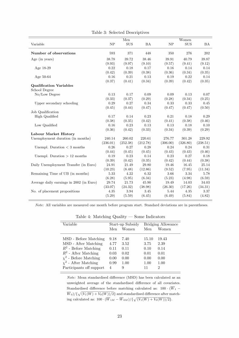
Table 3: Selected Descriptives

Men WomenVariable NP SUS BA NP SUS BA

Number of observations 593 371 448 350 276 202

Age (in years) 38.78 39.72 38.46 39.91 40.79 39.87(9.93) (9.97) (9.10) (9.57) (9.41) (9.12)

Age 18-29 0.22 0.18 0.17 0.16 0.14 0.14(0.42) (0.39) (0.38) (0.36) (0.34) (0.35)

Age 50-64 0.16 0.21 0.13 0.19 0.22 0.14(0.37) (0.41) (0.34) (0.39) (0.42) (0.35)

Qualification VariablesSchool Degree

No/Low Degree 0.13 0.17 0.09 0.09 0.13 0.07(0.33) (0.37) (0.29) (0.28) (0.34) (0.25)

Upper secondary schooling 0.29 0.27 0.34 0.33 0.33 0.45(0.45) (0.44) (0.47) (0.47) (0.47) (0.50)

Job QualificationHigh Qualified 0.17 0.14 0.23 0.21 0.18 0.29

(0.38) (0.35) (0.42) (0.41) (0.38) (0.46)Low Qualified 0.16 0.23 0.13 0.13 0.18 0.10

(0.36) (0.42) (0.33) (0.34) (0.39) (0.29)Labour Market HistoryUnemployment duration (in months) 240.14 260.02 220.61 276.77 301.28 229.92

(236.01) (252.38) (212.78) (306.00) (326.80) (238.51)Unempl. Duration < 3 months 0.26 0.27 0.28 0.24 0.24 0.31

(0.44) (0.45) (0.45) (0.43) (0.43) (0.46)Unempl. Duration > 12 months 0.19 0.23 0.14 0.23 0.27 0.18

(0.39) (0.42) (0.35) (0.42) (0.44) (0.38)Daily Unemployment Transfer (in Euro) 24.91 21.49 29.80 19.46 16.45 25.14

(10.23) (8.48) (12.86) (9.52) (7.95) (11.34)Remaining Time of UB (in months) 5.33 4.22 6.32 3.66 3.34 5.78

(6.28) (5.95) (6.34) (5.23) (4.98) (6.59)Average daily earnings in 2002 (in Euro) 29.74 21.73 45.90 19.49 14.03 34.03

(33.07) (24.32) (38.98) (26.30) (17.26) (34.31)No. of placement propositions 4.35 3.94 3.45 5.44 4.35 3.37

(5.29) (5.59) (6.45) (6.49) (5.84) (4.82)

Note: All variables are measured one month before program start. Standard deviations are in parentheses.

Table 4: Matching Quality — Some Indicators

Variable Start-up Subsidy Bridging AllowanceMen Women Men Women

MSD - Before Matching 9.18 7.40 15.10 19.43MSD - After Matching 4.77 3.52 3.75 2.39R2 - Before Matching 0.11 0.11 0.10 0.14R2 - After Matching 0.03 0.02 0.01 0.01χ2 - Before Matching 0.00 0.00 0.00 0.00χ2 - After Matching 0.99 1.00 1.00 1.00Participants off support 4 9 11 2

Note: Mean standardised difference (MSD) has been calculated as an

unweighted average of the standardised difference of all covariates.

Standardised difference before matching calculated as: 100 · (W 1 −W 0)/{

√(V1(W ) + V0(W ))/2} and standardised difference after match-

ing calculated as: 100 · (W 1M − W 0M )/{√

(V1(W ) + V0(W ))/2}.

23

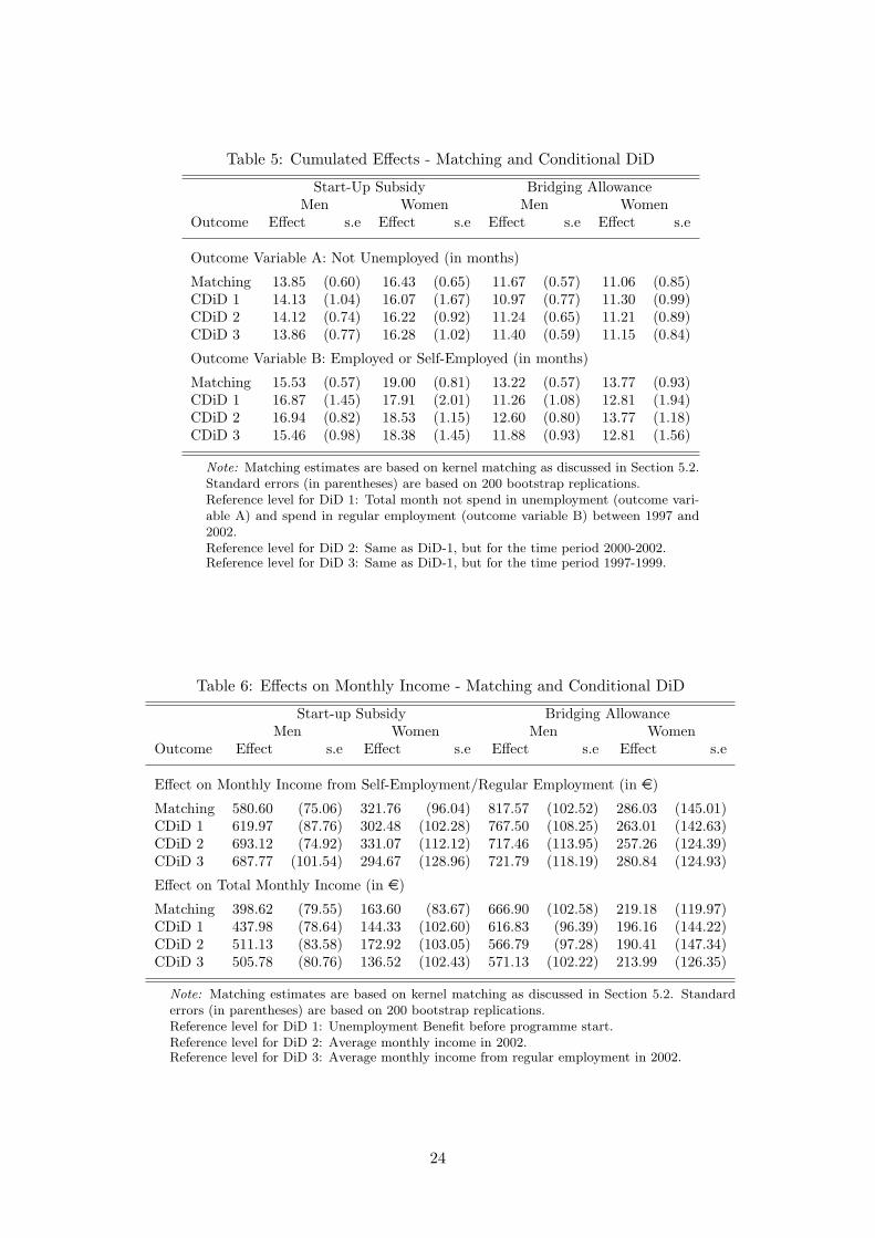
Table 5: Cumulated Effects - Matching and Conditional DiD

Start-Up Subsidy Bridging AllowanceMen Women Men Women

Outcome Effect s.e Effect s.e Effect s.e Effect s.e

Outcome Variable A: Not Unemployed (in months)

Matching 13.85 (0.60) 16.43 (0.65) 11.67 (0.57) 11.06 (0.85)CDiD 1 14.13 (1.04) 16.07 (1.67) 10.97 (0.77) 11.30 (0.99)CDiD 2 14.12 (0.74) 16.22 (0.92) 11.24 (0.65) 11.21 (0.89)CDiD 3 13.86 (0.77) 16.28 (1.02) 11.40 (0.59) 11.15 (0.84)

Outcome Variable B: Employed or Self-Employed (in months)


Note: Matching estimates are based on kernel matching as discussed in Section 5.2.Standard errors (in parentheses) are based on 200 bootstrap replications.Reference level for DiD 1: Total month not spend in unemployment (outcome vari-able A) and spend in regular employment (outcome variable B) between 1997 and2002.Reference level for DiD 2: Same as DiD-1, but for the time period 2000-2002.Reference level for DiD 3: Same as DiD-1, but for the time period 1997-1999.

Table 6: Effects on Monthly Income - Matching and Conditional DiD

Start-up Subsidy Bridging AllowanceMen Women Men Women

Outcome Effect s.e Effect s.e Effect s.e Effect s.e

Effect on Monthly Income from Self-Employment/Regular Employment (in e)


Effect on Total Monthly Income (in e)


Note: Matching estimates are based on kernel matching as discussed in Section 5.2. Standarderrors (in parentheses) are based on 200 bootstrap replications.Reference level for DiD 1: Unemployment Benefit before programme start.Reference level for DiD 2: Average monthly income in 2002.Reference level for DiD 3: Average monthly income from regular employment in 2002.

24

Table 7: Direct Employment Effects after 28 Months and FutureDevelopment1

Start-Up BridgingSubsidy Allowance

Men Women Men Women

Start-ups with employees 0.081 0.089 0.280 0.223(0.27) (0.29) (0.45) (0.42)

Number of employees (mean) 2.000 1.474 4.011 2.355(1.98) (0.77) (5.10) (1.40)

Share of regular employees 0.250 0.307 0.564 0.309(0.44) (0.45) (0.43) (0.39)

Employees in the future?Yes, surely 0.053 0.036 0.098 0.112

(0.23) (0.19) (0.30) (0.32)Rather yes 0.214 0.129 0.256 0.168

(0.41) (0.34) (0.44) (0.38)Rather no 0.359 0.335 0.342 0.206

(0.48) (0.47) (0.48) (0.41)No, by no means 0.374 0.500 0.303 0.514

(0.48) (0.50) (0.46) (0.50)

1 Numbers are shares unless stated otherwise; standard deviation in paren-

theses. Measured at the second interview after 28 months.

25

Figure 1: Distribution of the Propensity Scores – Common Support1

Men Women

Note: Propensity score is estimated according to the specification in Table A.1. Participants are depicted

in the upper half, nonparticipants in the lower half of each figure.

26

Figure 2: Treatment Effects over Time

Men Women

Outcome Variable A: Not Unemployed

Outcome variable B: Employed or Self-Employed

Note: Estimations are based on kernel matching as described in Section 5.2. Boot-

strapped standard errors are based on 200 replications.

27

Appendix

Table A.1: Propensity Score Estimation Results - Coefficientsa

SUS vs. Non-Participation BA vs. Non-ParticipationMen Women Men Women

Socio-demographic characteristicsAge category

25-29 0.184 0.375 −0.147 −0.25230-34 0.925∗ 0.746 0.463 0.0835-39 0.365 0.584 −0.003 0.15140-44 0.527 0.679 0.095 −0.1345-49 0.656 0.967+ −0.391 0.41250-64 1.422 ∗ ∗ 1.018∗ −0.107 −0.186

Children (Ref.: No children)One child 0.255 0 −0.028 −0.289Two or more children 0.484+ 0.051 −0.009 0.023

Qualification variablesSchool degree

Lower secondary schooling 0.433 −1.33 0.413 −1.173Middle secondary schooling 0.331 −1.376 0.381 −1.131Specialised upper sec. schooling 0.511 −0.992 0.147 −1.146Upper secondary schooling 0.342 −1.021 0.338 −1.196

Occupational group in previous profession (Ref.: manufacturing)Agriculture −0.251 0.095 −0.331 0.285Technical 0.508 0.945+ 0.199 1.357∗Services 0.271 0.369 −0.018 0.828+Other −0.274 0.031 −0.424 −0.121

Job QualificationIdiwquali0 −0.613+ −0.552 −0.344 −0.31Idiwquali1 −0.129 −0.862+ −0.241 −0.42Idiwquali2 −0.406∗ −0.209 −0.164 −0.282

Labour market historyDuration of last unemployment

3 months - < 6 months −0.458∗ −0.155 −0.366+ −0.3676 months - < 1 year −0.075 −0.33 0.134 −0.155≥ 1 year −0.032 0.017 0.111 0.155

With work experiences 0.295 −0.387 0.007 −0.198Number of placement propositions −0.016 −0.043∗ 0.004 −0.040+Unemployment benefits −0.044 ∗ ∗ −0.043 ∗ ∗ 0.026∗ 0.047 ∗ ∗Remaining benefit entitlement −0.032+ −0.054∗ −0.037∗ −0.029Daily income from regular employment

1999 0.001 0.002 0 0.0052000 −0.006 0.007 0.009 −0.0072001 0.012 −0.007 0.012+ 0.0042002 −0.018∗ −0.026 ∗ ∗ −0.005 −0.001

Constant −1.705 0.836 −0.711 −1.375Log-likelihood −570.413 −382.851 −642.031 −312.972Hit-Rate 41.805 48.182 45.521 42.5

Note: **/*/+ indicates significance at the 1%/5%/10% level.Additional variables included: Family status, health restrictions, nationality, desired working time, job qualifica-tion, months spend in regular employment and unemployment in the years 1999, 2000, 2001, and 2002, employmentstatus before unemployment, and dummy variables for the regional labour market context (strategy clusters). Fullestimation results and marginal effects are available on request by the authors.

28

Table A.2: Cross-Validation for the Bandwidth Selection

Start-Up Subsidy Bridging AllowanceMen Women Men Women

h RMSE h RMSE h RMSE h RMSE0.26977 0.49927 0.00091 0.52211 0.15221 0.49511 0.09469 0.491720.27977 0.49925 0.01091 0.47566 0.16221 0.49508 0.10469 0.491720.28977 0.49924 0.02091 0.48550 0.17221 0.49510 0.11469 0.491620.29977 0.49923 0.03091 0.49064 0.18221 0.49511 0.12469 0.491370.30977 0.49924 0.04091 0.49283 0.19221 0.49503 0.13469 0.491130.31977 0.49923 0.05091 0.49508 0.20221 0.49497 0.14469 0.490940.32977 0.49923 0.06091 0.49720 0.21221 0.49497 0.15469 0.490740.33977 0.49923 0.07091 0.49842 0.22221 0.49505 0.16469 0.490800.34977 0.49924 0.23221 0.49510 0.17469 0.490880.35977 0.49925 0.24221 0.49514 0.18469 0.490960.36977 0.49926 0.25221 0.49516 0.19469 0.49114

Note: We implement leave-one out cross-validation in a five step procedure (see, e.g.,Galdo, 2005):

1. Define a bandwidth search grid. Here, we use lbw + 0.05 × g for g = 0, 1, 2, ..., 20,where lbw = max[min[|P0i − P0−i|, |P0i − P0+i|]] is a lower bound defined by thepropensity score values of comparison group members in the support region.

2. Starting with the lowest bandwidth and using only the comparison sample, esti-mate the counterfactual outcome of each comparison unit using kernel matching onthe remaining N0 − 1 observations. Find the weighted MISE for that particularbandwidth.

3. Repeat step 2 for each of the remaining bandwidth values. Find the particularbandwidth h+ that minimizes the weighted MISE across all estimations.

4. Refine the bandwidth h+ by defining a +/−0.05 neighborhood around h+ and selecta new search grid.

5. Repeat steps 2 and 3 and select the bandwidth that yields the minimum weightedMISE among all estimations.

29

start-up subsidies in east germany: finally, a policy that works?

Documents