farm fragmentation, performance and subsidies in … · farm fragmentation, performance and...
TRANSCRIPT
FARM FRAGMENTATION,
PERFORMANCE AND
SUBSIDIES IN THE
EUROPEAN UNION Legrand SAINT-CYR
1, Laure LATRUFFE
1, Laurent PIET
1,
1 SMART, INRA, 35000, Rennes, France
29 December 2016
Public
D5.2D
agriXchange is funded by the European Commission’s 7th
ABOUT THE FLINT PROJECT
FLINT will provide an updated data-infrastructure needed by the agro-food sector and policy makers to provide up to date information on farm level indicators on sustainability and other new relevant issues. Better decision making will be facilitated by taking into account the sustainability performance of farms on a wide range of relevant topics, such as (1) market stabilization; (2) income support; (3) environmental sustainability; (4) climate change adaptation and mitigation; (5) innovation; and (6) resource efficiency. The approach will explicitly consider the heterogeneity of the farming sector in the EU and its member states. Together with the farming and agro-food sector the feasibility of these indicators will be determined.
FLINT will take into account the increasing needs for sustainability information by national and international retail and agro-food sectors. The FLINT approach is supported by the Sustainable Agriculture Initiative Platform and the Sustainability Consortium in which the agro-food sector actively participates. FLINT will establish a pilot network of at least 1000 farms (representative of farm diversity at EU level, including the different administrative environments in the different MS) that is well suited for the gathering of these data.
The lessons learned and recommendations from the empirical research conducted in 9 purposefully chosen MS will be used for estimating and discussing effects in all 28 MS. This will be very useful if the European Commission should decide to upgrade the pilot network to an operational EU-wide system.
PROJECT CONSORTIUM:
1 DLO Foundation (Stichting Dienst Landbouwkundig Onderzoek) Netherlands
2 AKI - Agrargazdasagi Kutato Intezet Hungary
3 LUKE Finland Finland
4 IERiGZ-PIB - Instytut Ekonomiki Rolnictwa i Gospodarki
Zywnosciowej-Panstwowy Instytut Badawcy Poland
5 INTIA - Instituto Navarro De Tecnologias e Infraestructuras Agrolimentarias Spain
6 ZALF - Leibniz Centre for Agricultural Landscape Research Germany
7 Teagasc - The Agriculture and Food Development Authority of Irelan Ireland
8 Demeter - Hellenic Agricultural Organization Greece
9 INRA - Institut National de la Recherche Agronomique France
10 CROP-R BV Netherlands
11 University of Hohenheim Germany
MORE INFORMATION:
Drs. Krijn Poppe (coordinator) e-mail: [email protected]
Dr. Hans Vrolijk e-mail: [email protected]
LEI Wageningen UR phone: +31 07 3358247
P.O. Box 29703
2502 LS The Hague www.flint-fp7.eu
The Netherlands
4 Farm fragmentation, performance and subsidies in the European Union
TABLE OF CONTENTS
List of tables ................................................................................................................................................. 5
List of acronyms............................................................................................................................................ 6
Executive summary ...................................................................................................................................... 7
1 Introduction .......................................................................................................................................... 8
2 Methodology and data ......................................................................................................................... 9
2.1 Data sources ................................................................................................................................ 9
2.2 Land fragmentation descriptors ................................................................................................ 10
2.3 Estimating the impact of subsidies on performance controlling for land fragmentation ......... 16
3 Results ................................................................................................................................................ 19
3.1 Results from the full sample ...................................................................................................... 19
3.2 Results from the sample with imputed data ............................................................................. 29
4 Conclusion .......................................................................................................................................... 36
5 References .......................................................................................................................................... 37
Farm fragmentation, performance and subsidies in the European Union 5
LIST OF TABLES Table 1: Total number of farms by country and main type of farming in the full sample ........................... 9
Table 2: Descriptive statistics of land fragmentation descriptors (full sample) ......................................... 12
Table 3: Descriptive statistics of land fragmentation descriptors by country ............................................ 13
Table 4: Descriptive statistics of land fragmentation descriptors by type of farming ............................... 14
Table 5: Descriptive statistics of indicators of working conditions and quality of life (full sample) .......... 14
Table 6: Correlation between land fragmentation descriptors and indicators of farmers’ working conditions and quality of life (full sample) ................................................................................................. 15
Table 7: Correlation between land fragmentation descriptors and working conditions and quality of life of farmers (for livestock farms) .................................................................................................................. 15
Table 8: Correlation between land fragmentation descriptors and working conditions and quality of life of farmers (for crop farms) ......................................................................................................................... 16
Table 9: Descriptive statistics of farm performance indicators (full sample)............................................. 17
Table 10: Descriptive statistics of the explanatory variables ..................................................................... 18
Table 11: Estimated parameters for model 1 (including total subsidies and excluding land fragmentation descriptors) – Full sample........................................................................................................................... 21
Table 12: Estimated parameters for model 2 (including total subsidies and land fragmentation descriptors): full sample ............................................................................................................................. 23
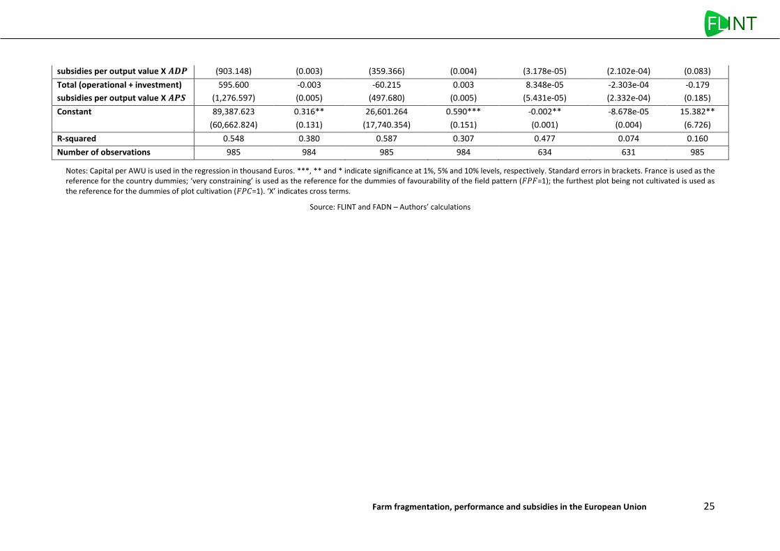
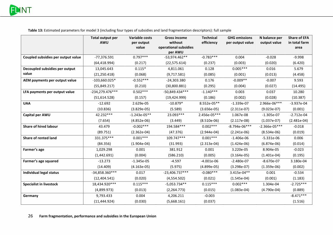
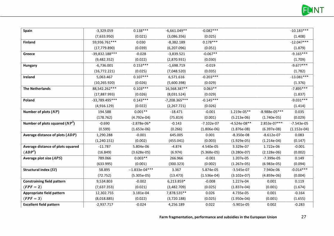
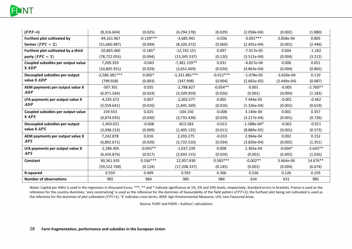
Table 13: Estimated parameters for model 3 (including four types of subsidies and land fragmentation descriptors): full sample ............................................................................................................................. 26
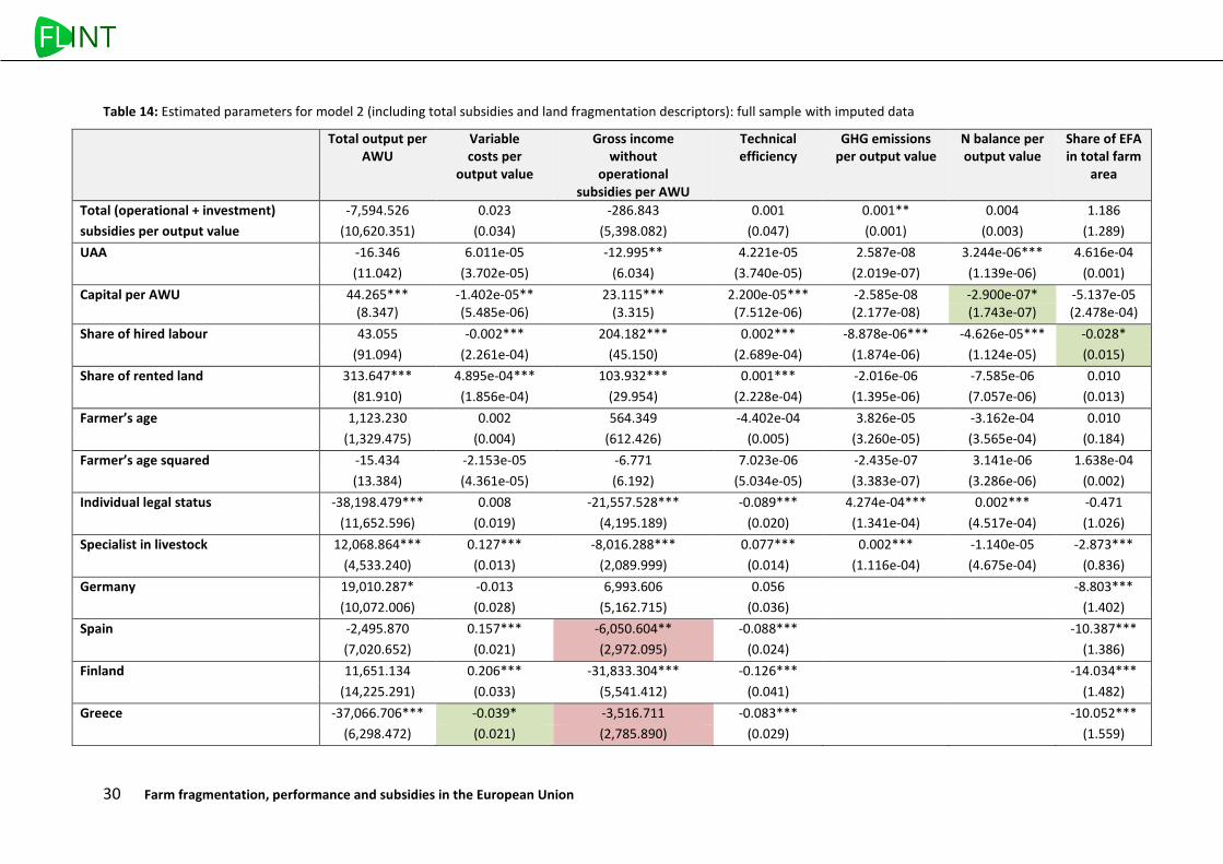
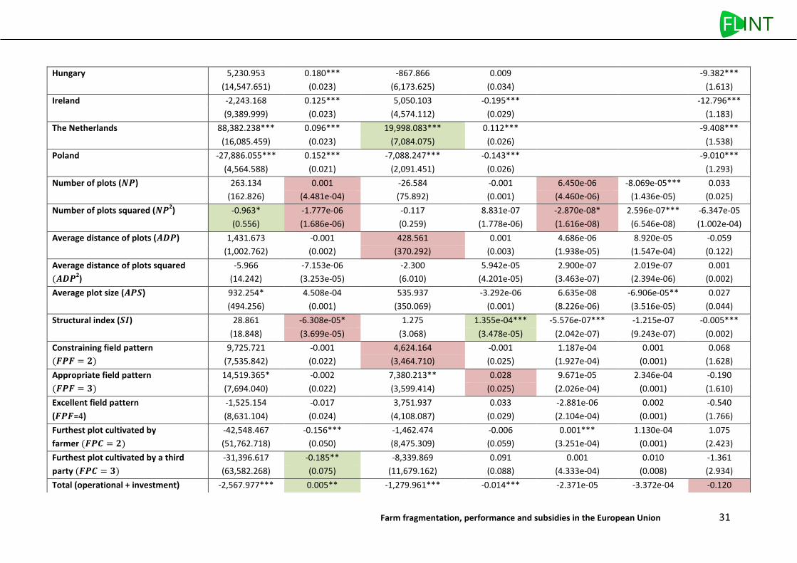
Table 14: Estimated parameters for model 2 (including total subsidies and land fragmentation descriptors): full sample with imputed data .............................................................................................. 30
Table 15: Estimated parameters for model 3 (including four types of subsidies and land fragmentation descriptors): full sample with imputed data .............................................................................................. 33
6 Farm fragmentation, performance and subsidies in the European Union
LIST OF ACRONYMS AEM Agri-environmental measure
AWU Annual working unit
CAP Common Agricultural Policy
DEA Data envelopment analysis
EFA Ecological focus areas
EU European Union
FADN Farm Accountancy Data Network
GHG Greenhouse gas
LF Land fragmentation
LFA Less favoured area
LPIS Land Parcel Identification System
SFP Single farm payment
UAA Utilised agricultural area
VRS Variable returns to scale
Farm fragmentation, performance and subsidies in the European Union 7
EXECUTIVE SUMMARY Recent studies have shown that there exists a significant relationship between land fragmentation (LF) and farm performance. However, it has been difficult so far to precisely assess this relationship on a large scale because there does not exist to date a single database which would allow to measure, at the same time and for the same farm, both performance and fragmentation indicators at the individual level. LF has yet to be taken into account since differences in LF may indeed be a source of difference in productivity or efficiency among farms which may appear as equivalent on other grounds. Not taking LF into account would lead to spuriously attribute its impact either to the farmers’ ability or to other variables of interest such as public support. It was one objective of the FLINT project to fill this gap and to provide consistent both LF and technical, economic and environmental performance data in an operational and tractable way for a sample of more than one thousand farms across nine countries of the European Union. The proposed analysis shows that the small set of LF-related variables surveyed in the FLINT project allows deriving sound LF indicators and thus effectively investigating the benefits of taking LF into account in the study of farm performance drivers. It especially reveals that LF seems to be only loosely related to working conditions and quality of life indicators for the studied sample, and that most of the impact of total subsidies, and more specifically of decoupled payments, seems to come from the interaction with the average distance of farm plots.
8 Farm fragmentation, performance and subsidies in the European Union
1 INTRODUCTION Some recent studies (Latruffe and Piet, 2014; Del Corral et al., 2011; Di Falco et al., 2010; Gonzalez et al., 2004) have shown that there exists a significant relationship between land fragmentation (LF) and various components of farm performance (production costs, physical yields, economic results, overall technical efficiency). However, it has been difficult so far to precisely assess this relationship on a large scale because there does not exist to date a single database which would allow to measure, at the same time and for the same farm, both performance and fragmentation indicators at the individual level. This is true worldwide and is especially the case in the European Union (EU). On the one hand, while they allow to precisely measure performance, standard accountancy data do not contain any information which would allow deriving even a proxy of land fragmentation. On the other hand, Land Parcel Identification Systems (LPIS), enforced by the European Council Regulation No 1593/2000, provide data which are not harmonized across Member States and do not allow measuring any components of farm performance. As Latruffe and Piet (2014) show, combining both datasets is not an easy task and suffers several drawbacks. This mainly arises because, due to confidentiality reasons, farms are not recorded with the same identifier in both databases, so that inputting one into the other ‘somehow’ leads to making assumptions and/or simplifications which may be detrimental to the robustness and scope of results; e.g., confronted to such a limitation in France, these authors resort to considering the role of ‘ambient’ land fragmentation only, under the assumption that the own land fragmentation of a farm is positively correlated with that of the municipality where it is located. As an alternative, gathering indicators on both dimensions at the same time and for the same farm needs to set up a specific survey which is inevitably limited in size, hence in scope.
Here we use data for a large sample of farms in the EU for which accountancy data as well as data on LF are available. The question here is whether farm subsidies, in particular those received in the frame of the Common Agricultural Policy (CAP), could be useful in enhancing farm (economic and environmental) performance, or if improvements in performance are constrained by the current field pattern of farms. If the latter is constraining, then the usefulness of CAP subsidies could be questioned, and the need of reallocating budget towards structural policies is also questioned. In other words, controlling for the impact of land fragmentation can help better single out the contribution of other major performance drivers such as the intrinsic behaviour of farmers and the impact of CAP subsidies.
Farm fragmentation, performance and subsidies in the European Union 9
2 METHODOLOGY AND DATA
2.1 Data sources
The analysis is based on a sample of farms of the Farm Accountancy Data Network (FADN) in several EU countries (The Netherlands, Hungary, Finland, Poland, Spain, Ireland, Greece, France and Germany). For this sample, FADN data are available (here after: ‘FADN data’) which contain accountancy and structural information at the farm level. For the same sample, additional farm-level data on economic, environmental and social sustainability of farms are available. These additional data, the ‘FLINT data’, were collected via face-to-face survey or merging of existing data, depending on the country. The FADN and FLINT data relate to accountancy year 2015, except for France and Germany for which it is 2014.
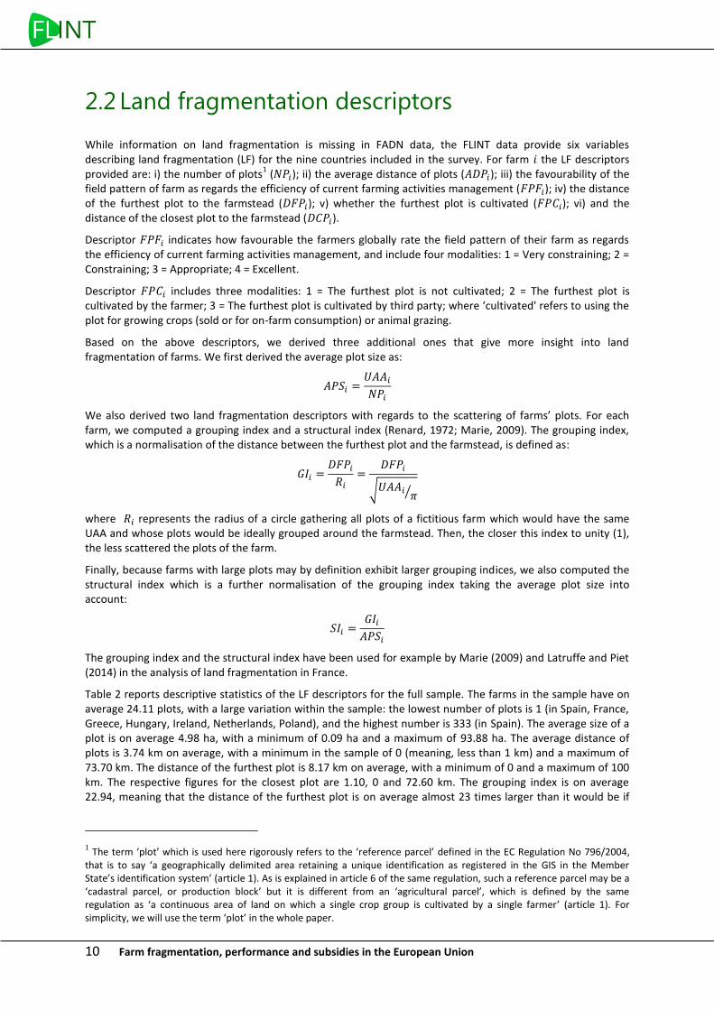
The sample considered includes farms which have a non-zero utilised agricultural area (UAA), and for which the information on fragmentation is available. Table 1 shows the number of farms in the sample considered, by country and by main type of farming, that is to say agricultural production specialisation. The sample consists of 1,053 farms, with a highest share of grazing livestock farms and then field crop farms.
Table 1: Total number of farms by country and main type of farming in the full sample
Main type of farming
Country
DE ES FI FR GR HU IE NL PL Total
Field crops 7 44 1 76 24 36 0 35 31 254
Horticulture 0 3 0 0 0 0 0 32 0 35
Permanent crops
6 3 0 60 69 0 0 0 26 164
Grazing livestock
20 63 45 96 29 8 53 53 26 393
Granivores 6 0 0 6 0 12 0 19 22 65
Mixed cropping
2 9 0 0 1 2 0 5 2 21
Mixed livestock
0 0 0 5 0 0 1 0 8 14
Mixed crops-livestock
8 1 3 33 0 29 0 2 31 107
Total 49 123 49 276 123 87 54 146 146 1,053
Notes: DE=Germany, ES=Spain, FI=Finland, FR=France, GR=Greece, HU=Hungary, IE=Ireland, NL=Netherlands, PL=Poland.
Source: FLINT and FADN – Authors’ calculations
10 Farm fragmentation, performance and subsidies in the European Union
2.2 Land fragmentation descriptors
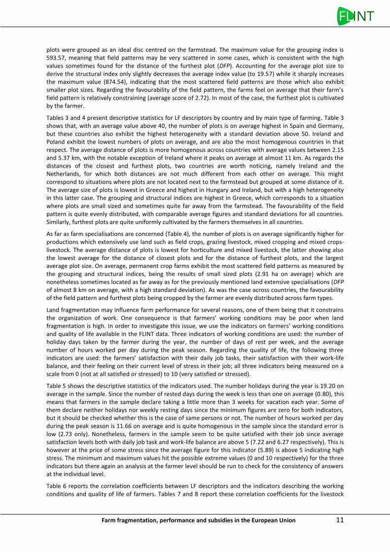
While information on land fragmentation is missing in FADN data, the FLINT data provide six variables describing land fragmentation (LF) for the nine countries included in the survey. For farm 𝑖 the LF descriptors provided are: i) the number of plots
1 (𝑁𝑃𝑖); ii) the average distance of plots (𝐴𝐷𝑃𝑖); iii) the favourability of the
field pattern of farm as regards the efficiency of current farming activities management (𝐹𝑃𝐹𝑖); iv) the distance of the furthest plot to the farmstead (𝐷𝐹𝑃𝑖); v) whether the furthest plot is cultivated (𝐹𝑃𝐶𝑖); vi) and the distance of the closest plot to the farmstead (𝐷𝐶𝑃𝑖).
Descriptor 𝐹𝑃𝐹𝑖 indicates how favourable the farmers globally rate the field pattern of their farm as regards the efficiency of current farming activities management, and include four modalities: 1 = Very constraining; 2 = Constraining; 3 = Appropriate; 4 = Excellent.
Descriptor 𝐹𝑃𝐶𝑖 includes three modalities: 1 = The furthest plot is not cultivated; 2 = The furthest plot is cultivated by the farmer; 3 = The furthest plot is cultivated by third party; where ‘cultivated' refers to using the plot for growing crops (sold or for on-farm consumption) or animal grazing.
Based on the above descriptors, we derived three additional ones that give more insight into land fragmentation of farms. We first derived the average plot size as:
𝐴𝑃𝑆𝑖 =𝑈𝐴𝐴𝑖
𝑁𝑃𝑖
We also derived two land fragmentation descriptors with regards to the scattering of farms’ plots. For each farm, we computed a grouping index and a structural index (Renard, 1972; Marie, 2009). The grouping index, which is a normalisation of the distance between the furthest plot and the farmstead, is defined as:
𝐺𝐼𝑖 =𝐷𝐹𝑃𝑖
𝑅𝑖
=𝐷𝐹𝑃𝑖
√𝑈𝐴𝐴𝑖𝜋⁄
where 𝑅𝑖 represents the radius of a circle gathering all plots of a fictitious farm which would have the same UAA and whose plots would be ideally grouped around the farmstead. Then, the closer this index to unity (1), the less scattered the plots of the farm.
Finally, because farms with large plots may by definition exhibit larger grouping indices, we also computed the structural index which is a further normalisation of the grouping index taking the average plot size into account:
𝑆𝐼𝑖 =𝐺𝐼𝑖
𝐴𝑃𝑆𝑖
The grouping index and the structural index have been used for example by Marie (2009) and Latruffe and Piet (2014) in the analysis of land fragmentation in France.
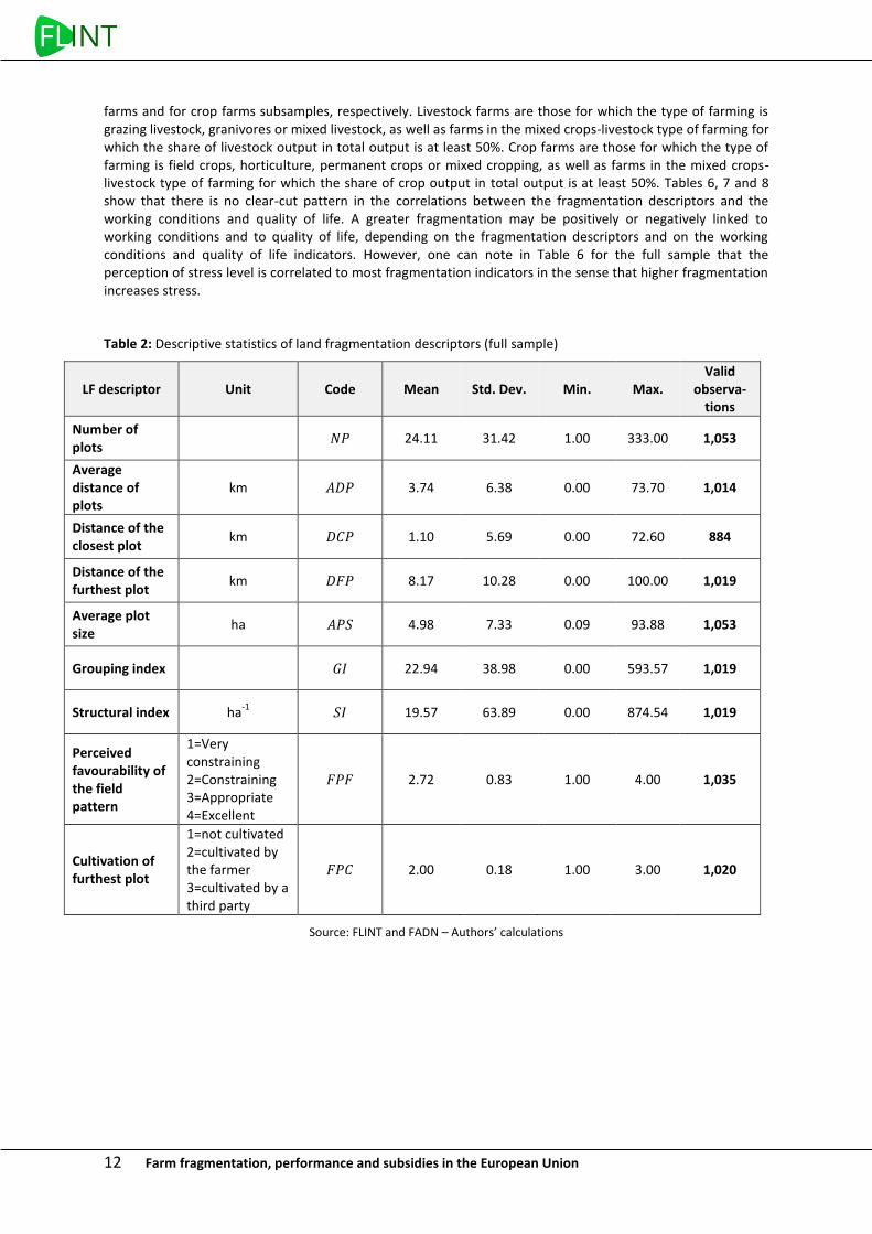
Table 2 reports descriptive statistics of the LF descriptors for the full sample. The farms in the sample have on average 24.11 plots, with a large variation within the sample: the lowest number of plots is 1 (in Spain, France, Greece, Hungary, Ireland, Netherlands, Poland), and the highest number is 333 (in Spain). The average size of a plot is on average 4.98 ha, with a minimum of 0.09 ha and a maximum of 93.88 ha. The average distance of plots is 3.74 km on average, with a minimum in the sample of 0 (meaning, less than 1 km) and a maximum of 73.70 km. The distance of the furthest plot is 8.17 km on average, with a minimum of 0 and a maximum of 100 km. The respective figures for the closest plot are 1.10, 0 and 72.60 km. The grouping index is on average 22.94, meaning that the distance of the furthest plot is on average almost 23 times larger than it would be if
1 The term ‘plot’ which is used here rigorously refers to the ‘reference parcel’ defined in the EC Regulation No 796/2004,
that is to say ‘a geographically delimited area retaining a unique identification as registered in the GIS in the Member State’s identification system’ (article 1). As is explained in article 6 of the same regulation, such a reference parcel may be a ‘cadastral parcel, or production block’ but it is different from an ‘agricultural parcel’, which is defined by the same regulation as ‘a continuous area of land on which a single crop group is cultivated by a single farmer’ (article 1). For simplicity, we will use the term ‘plot’ in the whole paper.
Farm fragmentation, performance and subsidies in the European Union 11
plots were grouped as an ideal disc centred on the farmstead. The maximum value for the grouping index is 593.57, meaning that field patterns may be very scattered in some cases, which is consistent with the high values sometimes found for the distance of the furthest plot (DFP). Accounting for the average plot size to derive the structural index only slightly decreases the average index value (to 19.57) while it sharply increases the maximum value (874.54), indicating that the most scattered field patterns are those which also exhibit smaller plot sizes. Regarding the favourability of the field pattern, the farms feel on average that their farm’s field pattern is relatively constraining (average score of 2.72). In most of the case, the furthest plot is cultivated by the farmer.
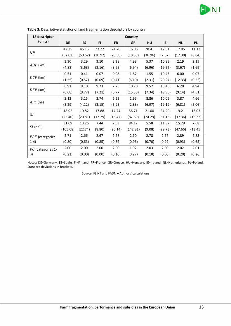
Tables 3 and 4 present descriptive statistics for LF descriptors by country and by main type of farming. Table 3 shows that, with an average value above 40, the number of plots is on average highest in Spain and Germany, but these countries also exhibit the highest heterogeneity with a standard deviation above 50. Ireland and Poland exhibit the lowest numbers of plots on average, and are also the most homogenous countries in that respect. The average distance of plots is more homogenous across countries with average values between 2.15 and 5.37 km, with the notable exception of Ireland where it peaks on average at almost 11 km. As regards the distances of the closest and furthest plots, two countries are worth noticing, namely Ireland and the Netherlands, for which both distances are not much different from each other on average. This might correspond to situations where plots are not located next to the farmstead but grouped at some distance of it. The average size of plots is lowest in Greece and highest in Hungary and Ireland, but with a high heterogeneity in this latter case. The grouping and structural indices are highest in Greece, which corresponds to a situation where plots are small sized and sometimes quite far away from the farmstead. The favourability of the field pattern is quite evenly distributed, with comparable average figures and standard deviations for all countries. Similarly, furthest plots are quite uniformly cultivated by the farmers themselves in all countries.
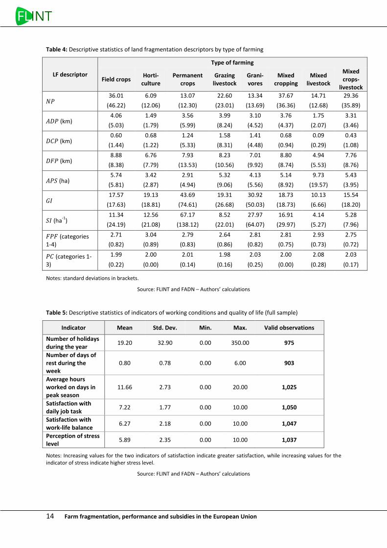
As far as farm specialisations are concerned (Table 4), the number of plots is on average significantly higher for productions which extensively use land such as field crops, grazing livestock, mixed cropping and mixed crops-livestock. The average distance of plots is lowest for horticulture and mixed livestock, the latter showing also the lowest average for the distance of closest plots and for the distance of furthest plots, and the largest average plot size. On average, permanent crop farms exhibit the most scattered field patterns as measured by the grouping and structural indices, being the results of small sized plots (2.91 ha on average) which are nonetheless sometimes located as far away as for the previously mentioned land extensive specialisations (DFP of almost 8 km on average, with a high standard deviation). As was the case across countries, the favourability of the field pattern and furthest plots being cropped by the farmer are evenly distributed across farm types.
Land fragmentation may influence farm performance for several reasons, one of them being that it constrains the organization of work. One consequence is that farmers’ working conditions may be poor when land fragmentation is high. In order to investigate this issue, we use the indicators on farmers’ working conditions and quality of life available in the FLINT data. Three indicators of working conditions are used: the number of holiday days taken by the farmer during the year, the number of days of rest per week, and the average number of hours worked per day during the peak season. Regarding the quality of life, the following three indicators are used: the farmers’ satisfaction with their daily job tasks, their satisfaction with their work-life balance, and their feeling on their current level of stress in their job; all three indicators being measured on a scale from 0 (not at all satisfied or stressed) to 10 (very satisfied or stressed).
Table 5 shows the descriptive statistics of the indicators used. The number holidays during the year is 19.20 on average in the sample. Since the number of rested days during the week is less than one on average (0.80), this means that farmers in the sample declare taking a little more than 3 weeks for vacation each year. Some of them declare neither holidays nor weekly resting days since the minimum figures are zero for both indicators, but it should be checked whether this is the case of same persons or not. The number of hours worked per day during the peak season is 11.66 on average and is quite homogenous in the sample since the standard error is low (2.73 only). Nonetheless, farmers in the sample seem to be quite satisfied with their job since average satisfaction levels both with daily job task and work-life balance are above 5 (7.22 and 6.27 respectively). This is however at the price of some stress since the average figure for this indicator (5.89) is above 5 indicating high stress. The minimum and maximum values hit the possible extreme values (0 and 10 respectively) for the three indicators but there again an analysis at the farmer level should be run to check for the consistency of answers at the individual level.
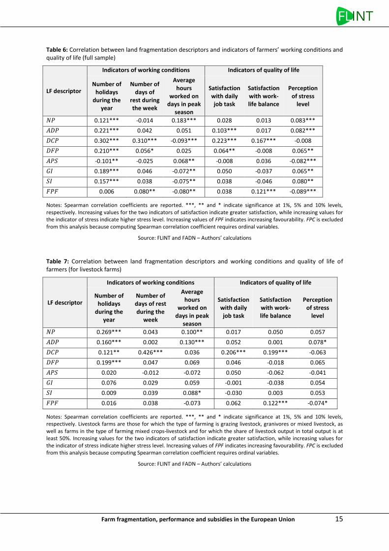
Table 6 reports the correlation coefficients between LF descriptors and the indicators describing the working conditions and quality of life of farmers. Tables 7 and 8 report these correlation coefficients for the livestock
12 Farm fragmentation, performance and subsidies in the European Union
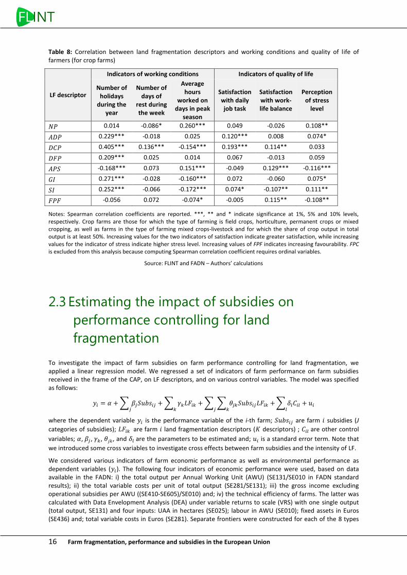
farms and for crop farms subsamples, respectively. Livestock farms are those for which the type of farming is grazing livestock, granivores or mixed livestock, as well as farms in the mixed crops-livestock type of farming for which the share of livestock output in total output is at least 50%. Crop farms are those for which the type of farming is field crops, horticulture, permanent crops or mixed cropping, as well as farms in the mixed crops-livestock type of farming for which the share of crop output in total output is at least 50%. Tables 6, 7 and 8 show that there is no clear-cut pattern in the correlations between the fragmentation descriptors and the working conditions and quality of life. A greater fragmentation may be positively or negatively linked to working conditions and to quality of life, depending on the fragmentation descriptors and on the working conditions and quality of life indicators. However, one can note in Table 6 for the full sample that the perception of stress level is correlated to most fragmentation indicators in the sense that higher fragmentation increases stress.
Table 2: Descriptive statistics of land fragmentation descriptors (full sample)
LF descriptor Unit Code Mean Std. Dev. Min. Max. Valid
observa-tions
Number of plots
𝑁𝑃 24.11 31.42 1.00 333.00 1,053
Average distance of plots
km 𝐴𝐷𝑃 3.74 6.38 0.00 73.70 1,014
Distance of the closest plot
km 𝐷𝐶𝑃 1.10 5.69 0.00 72.60 884
Distance of the furthest plot
km 𝐷𝐹𝑃 8.17 10.28 0.00 100.00 1,019
Average plot size
ha 𝐴𝑃𝑆 4.98 7.33 0.09 93.88 1,053
Grouping index 𝐺𝐼 22.94 38.98 0.00 593.57 1,019
Structural index ha-1
𝑆𝐼 19.57 63.89 0.00 874.54 1,019
Perceived favourability of the field pattern
1=Very constraining 2=Constraining 3=Appropriate 4=Excellent
𝐹𝑃𝐹 2.72 0.83 1.00 4.00 1,035
Cultivation of furthest plot
1=not cultivated 2=cultivated by the farmer 3=cultivated by a third party
𝐹𝑃𝐶 2.00 0.18 1.00 3.00 1,020
Source: FLINT and FADN – Authors’ calculations
Farm fragmentation, performance and subsidies in the European Union 13
Table 3: Descriptive statistics of land fragmentation descriptors by country
LF descriptor (units)
Country
DE ES FI FR GR HU IE NL PL
𝑁𝑃 42.25 45.15 33.22 24.78 16.06 28.41 12.51 17.05 11.12
(52.02) (59.62) (20.92) (20.38) (18.39) (36.96) (7.67) (17.38) (8.84)
𝐴𝐷𝑃 (km) 3.30 3.29 3.10 3.28 4.99 5.37 10.89 2.19 2.15
(4.83) (3.68) (2.16) (3.95) (6.94) (6.96) (19.52) (3.67) (1.69)
𝐷𝐶𝑃 (km) 0.51 0.41 0.07 0.08 1.87 1.55 10.45 6.00 0.07
(1.55) (0.57) (0.09) (0.41) (6.10) (2.31) (20.27) (12.33) (0.22)
𝐷𝐹𝑃 (km) 6.91 9.10 9.73 7.75 10.70 9.57 13.46 6.20 4.94
(6.68) (9.77) (7.21) (8.77) (15.38) (7.34) (19.95) (9.14) (4.51)
𝐴𝑃𝑆 (ha) 3.12 3.15 3.74 6.23 1.95 8.86 10.05 3.87 4.66
(3.29) (4.12) (3.15) (6.95) (2.83) (6.97) (19.19) (6.81) (5.06)
𝐺𝐼 18.92 19.82 17.88 14.74 56.71 21.00 34.20 19.21 16.03
(25.40) (20.81) (12.29) (15.47) (82.69) (24.29) (51.15) (37.36) (15.32)
𝑆𝐼 (ha-1
) 31.09 13.26 7.44 7.63 84.12 5.58 11.37 15.29 7.68
(105.68) (22.74) (8.80) (20.14) (142.81) (9.08) (29.73) (47.66) (13.45)
𝐹𝑃𝐹 (categories 1-4)
2.71 2.66 2.67 2.68 2.60 2.78 2.57 2.89 2.83
(0.80) (0.63) (0.85) (0.87) (0.96) (0.70) (0.92) (0.93) (0.65)
𝑃𝐶 (categories 1-3)
2.00 2.00 2.00 2.00 1.92 2.03 2.00 2.02 2.01
(0.21) (0.00) (0.00) (0.10) (0.27) (0.18) (0.00) (0.20) (0.26)
Notes: DE=Germany, ES=Spain, FI=Finland, FR=France, GR=Greece, HU=Hungary, IE=Ireland, NL=Netherlands, PL=Poland. Standard deviations in brackets.
Source: FLINT and FADN – Authors’ calculations
14 Farm fragmentation, performance and subsidies in the European Union
Table 4: Descriptive statistics of land fragmentation descriptors by type of farming
LF descriptor
Type of farming
Field crops Horti-
culture Permanent
crops Grazing
livestock Grani-vores
Mixed cropping
Mixed livestock
Mixed crops-
livestock
𝑁𝑃 36.01 6.09 13.07 22.60 13.34 37.67 14.71 29.36
(46.22) (12.06) (12.30) (23.01) (13.69) (36.36) (12.68) (35.89)
𝐴𝐷𝑃 (km) 4.06 1.49 3.56 3.99 3.10 3.76 1.75 3.31
(5.03) (1.79) (5.99) (8.24) (4.52) (4.37) (2.07) (3.46)
𝐷𝐶𝑃 (km) 0.60 0.68 1.24 1.58 1.41 0.68 0.09 0.43
(1.44) (1.22) (5.33) (8.31) (4.48) (0.94) (0.29) (1.08)
𝐷𝐹𝑃 (km) 8.88 6.76 7.93 8.23 7.01 8.80 4.94 7.76
(8.38) (7.79) (13.53) (10.56) (9.92) (8.74) (5.53) (8.76)
𝐴𝑃𝑆 (ha) 5.74 3.42 2.91 5.32 4.13 5.14 9.73 5.43
(5.81) (2.87) (4.94) (9.06) (5.56) (8.92) (19.57) (3.95)
𝐺𝐼 17.57 19.13 43.69 19.31 30.92 18.73 10.13 15.54
(17.63) (18.81) (74.61) (26.68) (50.03) (18.73) (6.66) (18.20)
𝑆𝐼 (ha-1
) 11.34 12.56 67.17 8.52 27.97 16.91 4.14 5.28
(24.19) (21.08) (138.12) (22.01) (64.07) (29.97) (5.27) (7.96)
𝐹𝑃𝐹 (categories 1-4)
2.71 3.04 2.79 2.64 2.81 2.81 2.93 2.75
(0.82) (0.89) (0.83) (0.86) (0.82) (0.75) (0.73) (0.72)
𝑃𝐶 (categories 1-3)
1.99 2.00 2.01 1.98 2.03 2.00 2.08 2.03
(0.22) (0.00) (0.14) (0.16) (0.25) (0.00) (0.28) (0.17)
Notes: standard deviations in brackets.
Source: FLINT and FADN – Authors’ calculations
Table 5: Descriptive statistics of indicators of working conditions and quality of life (full sample)
Indicator Mean Std. Dev. Min. Max. Valid observations
Number of holidays during the year
19.20 32.90 0.00 350.00 975
Number of days of rest during the week
0.80 0.78 0.00 6.00 903
Average hours worked on days in peak season
11.66 2.73 0.00 20.00 1,025
Satisfaction with daily job task
7.22 1.77 0.00 10.00 1,050
Satisfaction with work-life balance
6.27 2.18 0.00 10.00 1,047
Perception of stress level
5.89 2.35 0.00 10.00 1,037
Notes: Increasing values for the two indicators of satisfaction indicate greater satisfaction, while increasing values for the indicator of stress indicate higher stress level.
Source: FLINT and FADN – Authors’ calculations
Farm fragmentation, performance and subsidies in the European Union 15
Table 6: Correlation between land fragmentation descriptors and indicators of farmers’ working conditions and quality of life (full sample)
LF descriptor
Indicators of working conditions Indicators of quality of life
Number of holidays
during the year
Number of days of
rest during the week
Average hours
worked on days in peak
season
Satisfaction with daily job task
Satisfaction with work-life balance
Perception of stress
level
𝑁𝑃 0.121*** -0.014 0.183*** 0.028 0.013 0.083***
𝐴𝐷𝑃 0.221*** 0.042 0.051 0.103*** 0.017 0.082***
𝐷𝐶𝑃 0.302*** 0.310*** -0.093*** 0.223*** 0.167*** -0.008
𝐷𝐹𝑃 0.210*** 0.056* 0.025 0.064** -0.008 0.065**
𝐴𝑃𝑆 -0.101** -0.025 0.068** -0.008 0.036 -0.082***
𝐺𝐼 0.189*** 0.046 -0.072** 0.050 -0.037 0.065**
𝑆𝐼 0.157*** 0.038 -0.075** 0.038 -0.046 0.080**
𝐹𝑃𝐹 0.006 0.080** -0.080** 0.038 0.121*** -0.089***
Notes: Spearman correlation coefficients are reported. ***, ** and * indicate significance at 1%, 5% and 10% levels, respectively. Increasing values for the two indicators of satisfaction indicate greater satisfaction, while increasing values for the indicator of stress indicate higher stress level. Increasing values of FPF indicates increasing favourability. FPC is excluded from this analysis because computing Spearman correlation coefficient requires ordinal variables.
Source: FLINT and FADN – Authors’ calculations
Table 7: Correlation between land fragmentation descriptors and working conditions and quality of life of farmers (for livestock farms)
LF descriptor
Indicators of working conditions Indicators of quality of life
Number of holidays
during the year
Number of days of rest during the
week
Average hours
worked on days in peak
season
Satisfaction with daily job task
Satisfaction with work-life balance
Perception of stress
level
𝑁𝑃 0.269*** 0.043 0.100** 0.017 0.050 0.057
𝐴𝐷𝑃 0.160*** 0.002 0.130*** 0.052 0.001 0.078*
𝐷𝐶𝑃 0.121** 0.426*** 0.036 0.206*** 0.199*** -0.063
𝐷𝐹𝑃 0.199*** 0.047 0.069 0.046 -0.018 0.065
𝐴𝑃𝑆 0.020 -0.012 -0.072 0.050 -0.062 -0.041
𝐺𝐼 0.076 0.029 0.059 -0.001 -0.038 0.054
𝑆𝐼 0.009 0.039 0.088* -0.030 0.003 0.053
𝐹𝑃𝐹 0.016 0.038 -0.073 0.062 0.122*** -0.074*
Notes: Spearman correlation coefficients are reported. ***, ** and * indicate significance at 1%, 5% and 10% levels, respectively. Livestock farms are those for which the type of farming is grazing livestock, granivores or mixed livestock, as well as farms in the type of farming mixed crops-livestock and for which the share of livestock output in total output is at least 50%. Increasing values for the two indicators of satisfaction indicate greater satisfaction, while increasing values for the indicator of stress indicate higher stress level. Increasing values of FPF indicates increasing favourability. FPC is excluded from this analysis because computing Spearman correlation coefficient requires ordinal variables.
Source: FLINT and FADN – Authors’ calculations
16 Farm fragmentation, performance and subsidies in the European Union
Table 8: Correlation between land fragmentation descriptors and working conditions and quality of life of farmers (for crop farms)
LF descriptor
Indicators of working conditions Indicators of quality of life
Number of holidays
during the year
Number of days of
rest during the week
Average hours
worked on days in peak
season
Satisfaction with daily job task
Satisfaction with work-life balance
Perception of stress
level
𝑁𝑃 0.014 -0.086* 0.260*** 0.049 -0.026 0.108**
𝐴𝐷𝑃 0.229*** -0.018 0.025 0.120*** 0.008 0.074*
𝐷𝐶𝑃 0.405*** 0.136*** -0.154*** 0.193*** 0.114** 0.033
𝐷𝐹𝑃 0.209*** 0.025 0.014 0.067 -0.013 0.059
𝐴𝑃𝑆 -0.168*** 0.073 0.151*** -0.049 0.129*** -0.116***
𝐺𝐼 0.271*** -0.028 -0.160*** 0.072 -0.060 0.075*
𝑆𝐼 0.252*** -0.066 -0.172*** 0.074* -0.107** 0.111**
𝐹𝑃𝐹 -0.056 0.072 -0.074* -0.005 0.115** -0.108**
Notes: Spearman correlation coefficients are reported. ***, ** and * indicate significance at 1%, 5% and 10% levels, respectively. Crop farms are those for which the type of farming is field crops, horticulture, permanent crops or mixed cropping, as well as farms in the type of farming mixed crops-livestock and for which the share of crop output in total output is at least 50%. Increasing values for the two indicators of satisfaction indicate greater satisfaction, while increasing values for the indicator of stress indicate higher stress level. Increasing values of FPF indicates increasing favourability. FPC is excluded from this analysis because computing Spearman correlation coefficient requires ordinal variables.
Source: FLINT and FADN – Authors’ calculations
2.3 Estimating the impact of subsidies on
performance controlling for land
fragmentation
To investigate the impact of farm subsidies on farm performance controlling for land fragmentation, we applied a linear regression model. We regressed a set of indicators of farm performance on farm subsidies received in the frame of the CAP, on LF descriptors, and on various control variables. The model was specified as follows:
𝑦𝑖 = 𝛼 + ∑ 𝛽𝑗𝑆𝑢𝑏𝑠𝑖𝑗𝑗
+ ∑ 𝛾𝑘𝐿𝐹𝑖𝑘 + ∑ ∑ 𝜃𝑗𝑘𝑆𝑢𝑏𝑠𝑖𝑗𝐿𝐹𝑖𝑘𝑘
+𝑗
∑ 𝛿𝑙𝐶𝑖𝑙𝑙𝑘
+ 𝑢𝑖
where the dependent variable 𝑦𝑖 is the performance variable of the i-th farm; 𝑆𝑢𝑏𝑠𝑖𝑗 are farm 𝑖 subsidies (J
categories of subsidies); 𝐿𝐹𝑖𝑘 are farm 𝑖 land fragmentation descriptors (𝐾 descriptors) ; 𝐶𝑖𝑙 are other control
variables; 𝛼, 𝛽𝑗 , 𝛾𝑘, 𝜃𝑗𝑘, and 𝛿𝑙 are the parameters to be estimated and; 𝑢𝑖 is a standard error term. Note that
we introduced some cross variables to investigate cross effects between farm subsidies and the intensity of LF.
We considered various indicators of farm economic performance as well as environmental performance as dependent variables (𝑦𝑖). The following four indicators of economic performance were used, based on data available in the FADN: i) the total output per Annual Working Unit (AWU) (SE131/SE010 in FADN standard results); ii) the total variable costs per unit of total output (SE281/SE131); iii) the gross income excluding operational subsidies per AWU ((SE410-SE605)/SE010) and; iv) the technical efficiency of farms. The latter was calculated with Data Envelopment Analysis (DEA) under variable returns to scale (VRS) with one single output (total output, SE131) and four inputs: UAA in hectares (SE025); labour in AWU (SE010); fixed assets in Euros (SE436) and; total variable costs in Euros (SE281). Separate frontiers were constructed for each of the 8 types
Farm fragmentation, performance and subsidies in the European Union 17
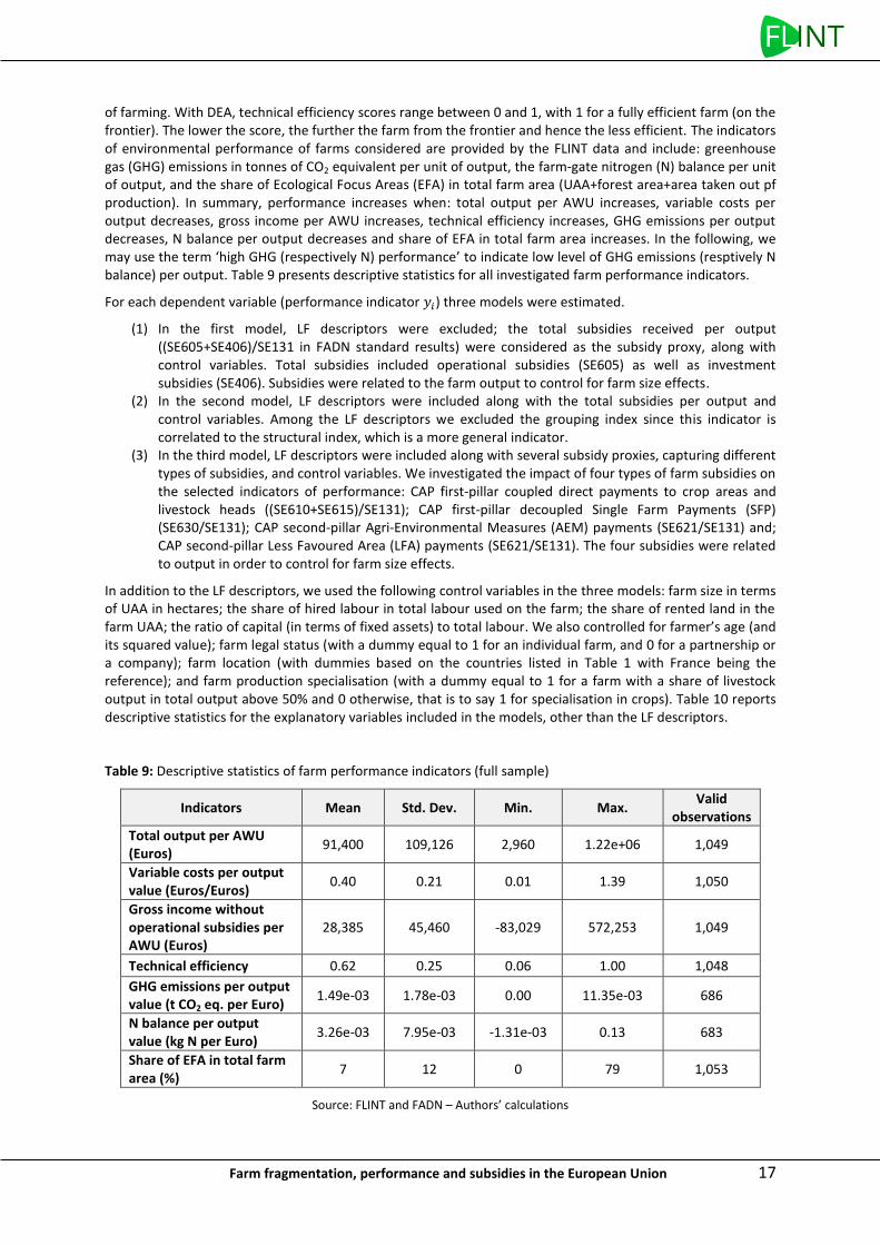
of farming. With DEA, technical efficiency scores range between 0 and 1, with 1 for a fully efficient farm (on the frontier). The lower the score, the further the farm from the frontier and hence the less efficient. The indicators of environmental performance of farms considered are provided by the FLINT data and include: greenhouse gas (GHG) emissions in tonnes of CO2 equivalent per unit of output, the farm-gate nitrogen (N) balance per unit of output, and the share of Ecological Focus Areas (EFA) in total farm area (UAA+forest area+area taken out pf production). In summary, performance increases when: total output per AWU increases, variable costs per output decreases, gross income per AWU increases, technical efficiency increases, GHG emissions per output decreases, N balance per output decreases and share of EFA in total farm area increases. In the following, we may use the term ‘high GHG (respectively N) performance’ to indicate low level of GHG emissions (resptively N balance) per output. Table 9 presents descriptive statistics for all investigated farm performance indicators.
For each dependent variable (performance indicator 𝑦𝑖) three models were estimated.
(1) In the first model, LF descriptors were excluded; the total subsidies received per output ((SE605+SE406)/SE131 in FADN standard results) were considered as the subsidy proxy, along with control variables. Total subsidies included operational subsidies (SE605) as well as investment subsidies (SE406). Subsidies were related to the farm output to control for farm size effects.
(2) In the second model, LF descriptors were included along with the total subsidies per output and control variables. Among the LF descriptors we excluded the grouping index since this indicator is correlated to the structural index, which is a more general indicator.
(3) In the third model, LF descriptors were included along with several subsidy proxies, capturing different types of subsidies, and control variables. We investigated the impact of four types of farm subsidies on the selected indicators of performance: CAP first-pillar coupled direct payments to crop areas and livestock heads ((SE610+SE615)/SE131); CAP first-pillar decoupled Single Farm Payments (SFP) (SE630/SE131); CAP second-pillar Agri-Environmental Measures (AEM) payments (SE621/SE131) and; CAP second-pillar Less Favoured Area (LFA) payments (SE621/SE131). The four subsidies were related to output in order to control for farm size effects.
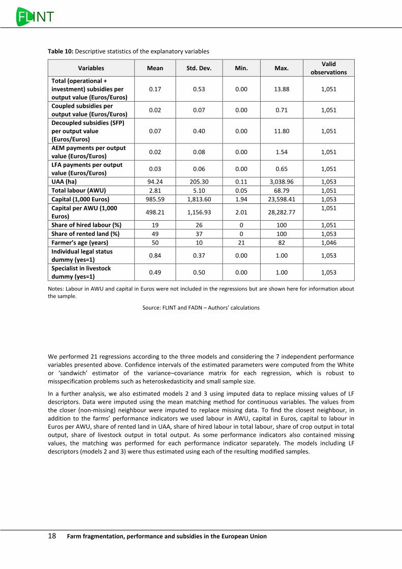
In addition to the LF descriptors, we used the following control variables in the three models: farm size in terms of UAA in hectares; the share of hired labour in total labour used on the farm; the share of rented land in the farm UAA; the ratio of capital (in terms of fixed assets) to total labour. We also controlled for farmer’s age (and its squared value); farm legal status (with a dummy equal to 1 for an individual farm, and 0 for a partnership or a company); farm location (with dummies based on the countries listed in Table 1 with France being the reference); and farm production specialisation (with a dummy equal to 1 for a farm with a share of livestock output in total output above 50% and 0 otherwise, that is to say 1 for specialisation in crops). Table 10 reports descriptive statistics for the explanatory variables included in the models, other than the LF descriptors.
Table 9: Descriptive statistics of farm performance indicators (full sample)
Indicators Mean Std. Dev. Min. Max. Valid
observations
Total output per AWU (Euros)
91,400 109,126 2,960 1.22e+06 1,049
Variable costs per output value (Euros/Euros)
0.40 0.21 0.01 1.39 1,050
Gross income without operational subsidies per AWU (Euros)
28,385 45,460 -83,029 572,253 1,049
Technical efficiency 0.62 0.25 0.06 1.00 1,048
GHG emissions per output value (t CO2 eq. per Euro)
1.49e-03 1.78e-03 0.00 11.35e-03 686
N balance per output value (kg N per Euro)
3.26e-03 7.95e-03 -1.31e-03 0.13 683
Share of EFA in total farm area (%)
7 12 0 79 1,053
Source: FLINT and FADN – Authors’ calculations
18 Farm fragmentation, performance and subsidies in the European Union
Table 10: Descriptive statistics of the explanatory variables
Variables Mean Std. Dev. Min. Max. Valid
observations
Total (operational + investment) subsidies per output value (Euros/Euros)
0.17 0.53 0.00 13.88 1,051
Coupled subsidies per output value (Euros/Euros)
0.02 0.07 0.00 0.71 1,051
Decoupled subsidies (SFP) per output value (Euros/Euros)
0.07 0.40 0.00 11.80 1,051
AEM payments per output value (Euros/Euros)
0.02 0.08 0.00 1.54 1,051
LFA payments per output value (Euros/Euros)
0.03 0.06 0.00 0.65 1,051
UAA (ha) 94.24 205.30 0.11 3,038.96 1,053
Total labour (AWU) 2.81 5.10 0.05 68.79 1,051
Capital (1,000 Euros) 985.59 1,813.60 1.94 23,598.41 1,053
Capital per AWU (1,000 Euros)
498.21 1,156.93 2.01 28,282.77 1,051
Share of hired labour (%) 19 26 0 100 1,051
Share of rented land (%) 49 37 0 100 1,053
Farmer’s age (years) 50 10 21 82 1,046
Individual legal status dummy (yes=1)
0.84 0.37 0.00 1.00 1,053
Specialist in livestock dummy (yes=1)
0.49 0.50 0.00 1.00 1,053
Notes: Labour in AWU and capital in Euros were not included in the regressions but are shown here for information about the sample.
Source: FLINT and FADN – Authors’ calculations
We performed 21 regressions according to the three models and considering the 7 independent performance variables presented above. Confidence intervals of the estimated parameters were computed from the White or ‘sandwich’ estimator of the variance–covariance matrix for each regression, which is robust to misspecification problems such as heteroskedasticity and small sample size.
In a further analysis, we also estimated models 2 and 3 using imputed data to replace missing values of LF descriptors. Data were imputed using the mean matching method for continuous variables. The values from the closer (non-missing) neighbour were imputed to replace missing data. To find the closest neighbour, in addition to the farms’ performance indicators we used labour in AWU, capital in Euros, capital to labour in Euros per AWU, share of rented land in UAA, share of hired labour in total labour, share of crop output in total output, share of livestock output in total output. As some performance indicators also contained missing values, the matching was performed for each performance indicator separately. The models including LF descriptors (models 2 and 3) were thus estimated using each of the resulting modified samples.
Farm fragmentation, performance and subsidies in the European Union 19
3 RESULTS
3.1 Results from the full sample
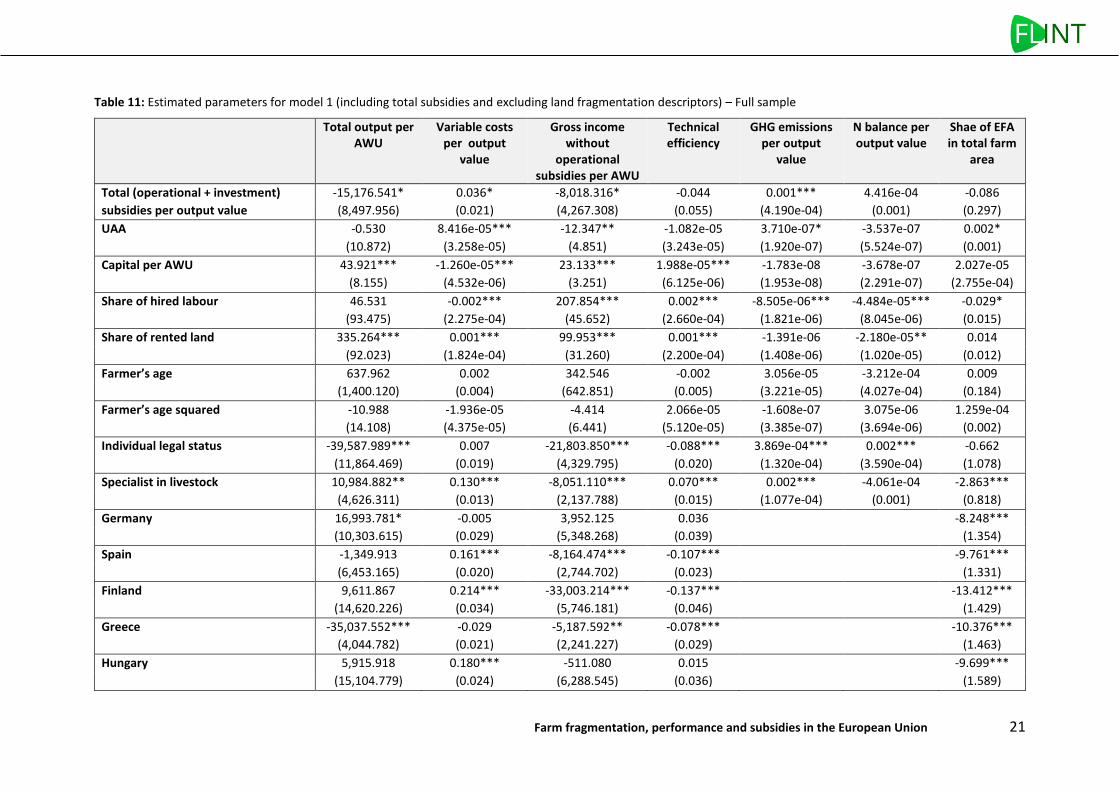
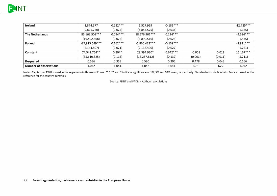
Tables 11, 12 and 13 report the estimated parameters for models 1 (with total subsidies proxy and without LF descriptors), 2 (with total subsidies proxy and LF descriptors) and 3 (with four types of subsidies proxies and LF descriptors), respectively.
Results from Table 11 (model 1) show that public support, in terms of total subsidies (operational and investment) received per Euro of output, has a negative impact on economic performance of farms except for technical efficiency for which the impact is not significant. Thus, public support decreases labour productivity (in terms of output per AWU) and gross income per AWU, and increases the costs of variable inputs to produce the same amount of output. Public support has also a deteriorating impact on GHG emissions per Euro of output by increasing them, but has no significant impact on the N balance per output nor on the share of EFA in total farm area.
As regards to the other explanatory variables, the results in Table 11 show that farm size in terms of total UAA has a significant negative impact on two economic performance indicators (variable costs per output and gross income per AWU) and on one environmental performance indicators (GHG emissions) but a positive effect on the share of EFA in total farm area. The technology, proxied by the capital to labour ratio, has a significant positive effect on all economic performance indicators, but no significant effect on the environmental performance indicators. The share of hired labour is favourable to all economic performance indicators, except for total output per AWU for which there is no significant effect and for the share of EFA in total farm area for which the effect is significantly negative. The share of rented land is favourable to all economic performance indicators, except for variable costs for which the sign of the parameter is positive indicating a negative effect on performance, and to N balance per output. Farmer’s age has no significant impact on performance. The individual legal status is generally not favourable to performance: farms operated under individual legal status are lower economically and environmentally performers, except when variable costs per output and the share of EFA in total farm area are considered, for which the effect is not significant. Finally, farms specialised in livestock are better performers in terms of total output per AWU, technical efficiency and share of EFA in total farm area, while farms specialised in crops are better performers in terms of variable costs per output, gross income per AWU and GHG emissions per output.
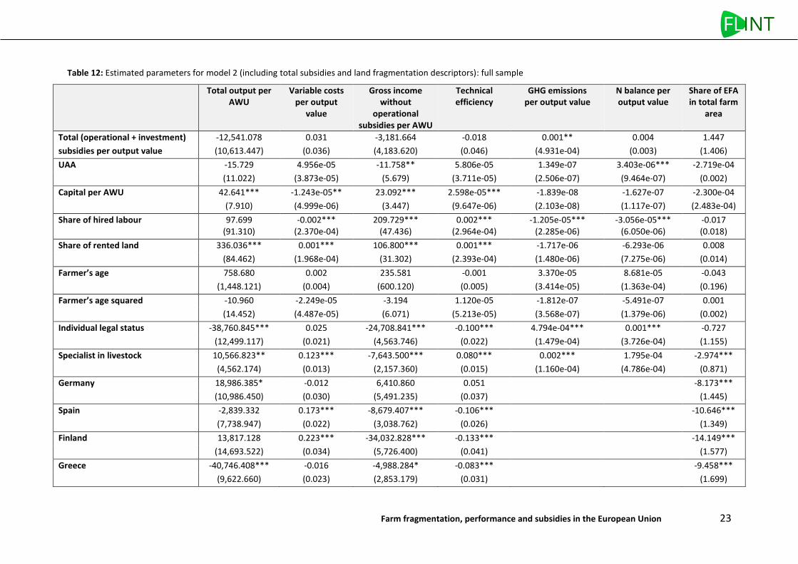
Results from Table 12 (model 2) show that, when controlling for LF in the regressions, total subsidies per output have no effect anymore per se (except when GHG emissions per output are concerned), but their effect is channelled through the indicators of LF. More precisely, the subsidy proxy has no significant effect on the performance indicators (except for GHG emissions per output for which the positive effect on the emissions shown in Table 11 is confirmed. But the cross term with the average distance of plots has an effect on all economic indicators and on the share of EFA in total farm area. With this cross term, the negative impact of the subsidy proxy on farm economic performance (in terms total output per AWU, variable costs per output, gross income per AWU) as shown in Table 11 is confirmed. The cross term also shows a significant negative effect on technical efficiency and a negative effect on the EFA proxy (i.e., a negative effect on environmental performance in terms of EFA). In other words, the furthest the average distance of plots, the greater the negative effect of the subsidy proxy on economic performance and EFA performance. By contrast, the cross term of the subsidy proxy with the average plot size has no significant effect on any performance indicator.
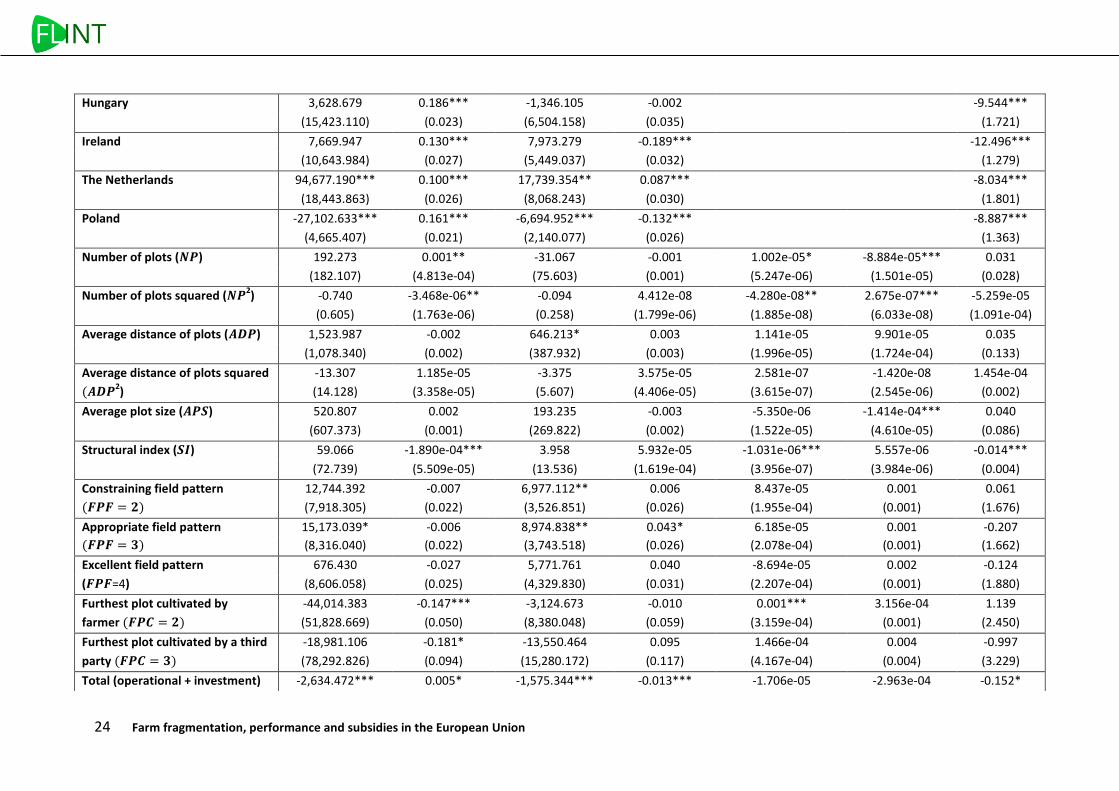
Focusing on LF indicators, results in Table 12 show that the total number of plot has a positive impact on the
total variable costs per output and on GHG emissions per output, that is to say a negative impact on economic
and environmental performance captured with these proxies. This result can be explained by the positive
correlation between the farm number of plots and the farm size. Farm tends to use more inputs when the
operated size increases. However, the effect is reverse for N balance per output: the number of plots decreases
the N balance. The nonlinear impact shown by the number of plots squared, suggests that the impact of the
number of plots on the variable costs per output and on GHG emissions per output decreases when the
20 Farm fragmentation, performance and subsidies in the European Union
number of plots becomes large, while it increases for N balance. The average distance of plots has a significant
effect on gross income per AWU, the effect being positive. The average plot size has a significant effect on N
balance, reducing it. The structural index has a significant and negative impact on the total variable costs per
output and the GHG emissions per output. As regard the negative impact on the variable costs per output, this
result could be explained by the fact that LF may give greater opportunity to increase total output with regards
to the total inputs used by cropping diversification (Manjunatha, 2012) and risk reduction (Blarel et al., 1992;
Kawasaki, 2010; Latruffe and Piet, 2014). For example, when plots are distant to each other, the farm may
benefit from soil quality and thus may use fewer inputs especially in terms of fertilisers. Scattered plots may be
also more convenient to avoid propagation of crops’ diseases and pests leading to a lower use of pesticides.
Results from Table 13 (model 3) where LF is also controlled for but considering four types of subsidies, show
that the coupled subsidy proxy has a significant negative effect on farm economic performance in terms of
variable costs per output, gross income per AWU (reinforced for a high average distance of plots) and technical
efficiency, and no significant effect on environmental performance. Decoupled subsidies significantly increase
variable costs per output (an effect that is reinforced for a high average distance of plots) and GHG emissions
per output (an effect that is reduced for a high average plot size). The negative effect on economic
performance shown for variable costs per output is also evident for the three other economic performance
indicators when the decoupled subsidy proxy is related to the average distance of plots. The AEM payment
proxy has a negative effect on total output per AWU, on variable costs per output and on GHG emissions per
output. When related to the average distance of plots, it also has a negative effect on technical efficiency and
share of EFA in total farm area. Finally, the LFA payment proxy has a negative effect on economic performance
whatever the indicator considered, and the effect on variable costs per output is reinforced with the average
plot size. This subsidy proxy also has a significant effect on environmental performance when it is related to the
average plot size: it reduces N balance and the share of EFA in total farm area.
In summary, economic performance indicators are almost all affected negatively by total subsidies and by all
four types of subsidies, whether alone or interacted with LF descriptors. One notable exception is the
decreasing effect of the AEM payment proxy on the variable costs per ouput (hence a positive effect on
economic performance). As for environmental performance, GHG emissions are increased by total subsidies
and decoupled subsidies, but the effect of the latter is reduced for high average plot size. By contrast, GHG
emissions are reduced by AEM payments. N balance is not affected by subsidies, except for a negative effect of
LFA payments interacted with average plot size. Similarly, the share of EFA in total farm area is not affected by
subsidies, except for a negative effect of AEM payments interacted with average distance of plot and a negative
effect of LFA interacted with average plot size.
Farm fragmentation, performance and subsidies in the European Union 21
Table 11: Estimated parameters for model 1 (including total subsidies and excluding land fragmentation descriptors) – Full sample
Total output per AWU
Variable costs per output
value
Gross income without
operational subsidies per AWU
Technical efficiency
GHG emissions per output
value
N balance per output value
Shae of EFA in total farm
area
Total (operational + investment) -15,176.541* 0.036* -8,018.316* -0.044 0.001*** 4.416e-04 -0.086
subsidies per output value (8,497.956) (0.021) (4,267.308) (0.055) (4.190e-04) (0.001) (0.297)
UAA -0.530 8.416e-05*** -12.347** -1.082e-05 3.710e-07* -3.537e-07 0.002*
(10.872) (3.258e-05) (4.851) (3.243e-05) (1.920e-07) (5.524e-07) (0.001)
Capital per AWU 43.921*** -1.260e-05*** 23.133*** 1.988e-05*** -1.783e-08 -3.678e-07 2.027e-05
(8.155) (4.532e-06) (3.251) (6.125e-06) (1.953e-08) (2.291e-07) (2.755e-04)
Share of hired labour 46.531 -0.002*** 207.854*** 0.002*** -8.505e-06*** -4.484e-05*** -0.029*
(93.475) (2.275e-04) (45.652) (2.660e-04) (1.821e-06) (8.045e-06) (0.015)
Share of rented land 335.264*** 0.001*** 99.953*** 0.001*** -1.391e-06 -2.180e-05** 0.014
(92.023) (1.824e-04) (31.260) (2.200e-04) (1.408e-06) (1.020e-05) (0.012)
Farmer’s age 637.962 0.002 342.546 -0.002 3.056e-05 -3.212e-04 0.009
(1,400.120) (0.004) (642.851) (0.005) (3.221e-05) (4.027e-04) (0.184)
Farmer’s age squared -10.988 -1.936e-05 -4.414 2.066e-05 -1.608e-07 3.075e-06 1.259e-04
(14.108) (4.375e-05) (6.441) (5.120e-05) (3.385e-07) (3.694e-06) (0.002)
Individual legal status -39,587.989*** 0.007 -21,803.850*** -0.088*** 3.869e-04*** 0.002*** -0.662
(11,864.469) (0.019) (4,329.795) (0.020) (1.320e-04) (3.590e-04) (1.078)
Specialist in livestock 10,984.882** 0.130*** -8,051.110*** 0.070*** 0.002*** -4.061e-04 -2.863***
(4,626.311) (0.013) (2,137.788) (0.015) (1.077e-04) (0.001) (0.818)
Germany 16,993.781* -0.005 3,952.125 0.036 -8.248***
(10,303.615) (0.029) (5,348.268) (0.039) (1.354)
Spain -1,349.913 0.161*** -8,164.474*** -0.107*** -9.761***
(6,453.165) (0.020) (2,744.702) (0.023) (1.331)
Finland 9,611.867 0.214*** -33,003.214*** -0.137*** -13.412***
(14,620.226) (0.034) (5,746.181) (0.046) (1.429)
Greece -35,037.552*** -0.029 -5,187.592** -0.078*** -10.376***
(4,044.782) (0.021) (2,241.227) (0.029) (1.463)
Hungary 5,915.918 0.180*** -511.080 0.015 -9.699***
(15,104.779) (0.024) (6,288.545) (0.036) (1.589)
22 Farm fragmentation, performance and subsidies in the European Union
Ireland 1,874.577 0.132*** 6,527.969 -0.189*** -12.725***
(9,821.270) (0.025) (4,853.575) (0.034) (1.185)
The Netherlands 85,163.509*** 0.094*** 18,576.901*** 0.124*** -9.684***
(16,402.568) (0.022) (6,890.516) (0.026) (1.535)
Poland -27,915.549*** 0.162*** -6,860.422*** -0.139*** -8.921***
(5,144.807) (0.021) (2,138.490) (0.027) (1.261)
Constant 74,542.754** 0.204* 28,594.920* 0.642*** -0.001 0.012 15.167***
(35,610.825) (0.113) (16,287.812) (0.132) (0.001) (0.011) (5.211)
R-squared 0.536 0.359 0.580 0.306 0.478 0.043 0.166
Number of observations 1,042 1,041 1,042 1,041 678 675 1,042
Notes: Capital per AWU is used in the regression in thousand Euros. ***, ** and * indicate significance at 1%, 5% and 10% levels, respectively. Standard errors in brackets. France is used as the reference for the country dummies.
Source: FLINT and FADN – Authors’ calculations
Farm fragmentation, performance and subsidies in the European Union 23
Table 12: Estimated parameters for model 2 (including total subsidies and land fragmentation descriptors): full sample
Total output per AWU
Variable costs per output
value
Gross income without
operational subsidies per AWU
Technical efficiency
GHG emissions per output value
N balance per output value
Share of EFA in total farm
area
Total (operational + investment) -12,541.078 0.031 -3,181.664 -0.018 0.001** 0.004 1.447
subsidies per output value (10,613.447) (0.036) (4,183.620) (0.046) (4.931e-04) (0.003) (1.406)
UAA -15.729 4.956e-05 -11.758** 5.806e-05 1.349e-07 3.403e-06*** -2.719e-04
(11.022) (3.873e-05) (5.679) (3.711e-05) (2.506e-07) (9.464e-07) (0.002)
Capital per AWU 42.641*** -1.243e-05** 23.092*** 2.598e-05*** -1.839e-08 -1.627e-07 -2.300e-04
(7.910) (4.999e-06) (3.447) (9.647e-06) (2.103e-08) (1.117e-07) (2.483e-04)
Share of hired labour 97.699 -0.002*** 209.729*** 0.002*** -1.205e-05*** -3.056e-05*** -0.017 (91.310) (2.370e-04) (47.436) (2.964e-04) (2.285e-06) (6.050e-06) (0.018)
Share of rented land 336.036*** 0.001*** 106.800*** 0.001*** -1.717e-06 -6.293e-06 0.008
(84.462) (1.968e-04) (31.302) (2.393e-04) (1.480e-06) (7.275e-06) (0.014)
Farmer’s age 758.680 0.002 235.581 -0.001 3.370e-05 8.681e-05 -0.043
(1,448.121) (0.004) (600.120) (0.005) (3.414e-05) (1.363e-04) (0.196)
Farmer’s age squared -10.960 -2.249e-05 -3.194 1.120e-05 -1.812e-07 -5.491e-07 0.001
(14.452) (4.487e-05) (6.071) (5.213e-05) (3.568e-07) (1.379e-06) (0.002)
Individual legal status -38,760.845*** 0.025 -24,708.841*** -0.100*** 4.794e-04*** 0.001*** -0.727
(12,499.117) (0.021) (4,563.746) (0.022) (1.479e-04) (3.726e-04) (1.155)
Specialist in livestock 10,566.823** 0.123*** -7,643.500*** 0.080*** 0.002*** 1.795e-04 -2.974***
(4,562.174) (0.013) (2,157.360) (0.015) (1.160e-04) (4.786e-04) (0.871)
Germany 18,986.385* -0.012 6,410.860 0.051 -8.173***
(10,986.450) (0.030) (5,491.235) (0.037) (1.445)
Spain -2,839.332 0.173*** -8,679.407*** -0.106*** -10.646***
(7,738.947) (0.022) (3,038.762) (0.026) (1.349)
Finland 13,817.128 0.223*** -34,032.828*** -0.133*** -14.149***
(14,693.522) (0.034) (5,726.400) (0.041) (1.577)
Greece -40,746.408*** -0.016 -4,988.284* -0.083*** -9.458***
(9,622.660) (0.023) (2,853.179) (0.031) (1.699)
24 Farm fragmentation, performance and subsidies in the European Union
Hungary 3,628.679 0.186*** -1,346.105 -0.002 -9.544***
(15,423.110) (0.023) (6,504.158) (0.035) (1.721)
Ireland 7,669.947 0.130*** 7,973.279 -0.189*** -12.496***
(10,643.984) (0.027) (5,449.037) (0.032) (1.279)
The Netherlands 94,677.190*** 0.100*** 17,739.354** 0.087*** -8.034***
(18,443.863) (0.026) (8,068.243) (0.030) (1.801)
Poland -27,102.633*** 0.161*** -6,694.952*** -0.132*** -8.887***
(4,665.407) (0.021) (2,140.077) (0.026) (1.363)
Number of plots (𝑵𝑷) 192.273 0.001** -31.067 -0.001 1.002e-05* -8.884e-05*** 0.031
(182.107) (4.813e-04) (75.603) (0.001) (5.247e-06) (1.501e-05) (0.028)
Number of plots squared (𝑵𝑷2) -0.740 -3.468e-06** -0.094 4.412e-08 -4.280e-08** 2.675e-07*** -5.259e-05
(0.605) (1.763e-06) (0.258) (1.799e-06) (1.885e-08) (6.033e-08) (1.091e-04)
Average distance of plots (𝑨𝑫𝑷) 1,523.987 -0.002 646.213* 0.003 1.141e-05 9.901e-05 0.035
(1,078.340) (0.002) (387.932) (0.003) (1.996e-05) (1.724e-04) (0.133)
Average distance of plots squared -13.307 1.185e-05 -3.375 3.575e-05 2.581e-07 -1.420e-08 1.454e-04
(𝑨𝑫𝑷2)
(14.128) (3.358e-05) (5.607) (4.406e-05) (3.615e-07) (2.545e-06) (0.002)
Average plot size (𝑨𝑷𝑺) 520.807 0.002 193.235 -0.003 -5.350e-06 -1.414e-04*** 0.040
(607.373) (0.001) (269.822) (0.002) (1.522e-05) (4.610e-05) (0.086)
Structural index (𝑺𝑰) 59.066 -1.890e-04*** 3.958 5.932e-05 -1.031e-06*** 5.557e-06 -0.014***
(72.739) (5.509e-05) (13.536) (1.619e-04) (3.956e-07) (3.984e-06) (0.004)
Constraining field pattern 12,744.392 -0.007 6,977.112** 0.006 8.437e-05 0.001 0.061
(𝑭𝑷𝑭 = 𝟐) (7,918.305) (0.022) (3,526.851) (0.026) (1.955e-04) (0.001) (1.676)
Appropriate field pattern 15,173.039* -0.006 8,974.838** 0.043* 6.185e-05 0.001 -0.207
(𝑭𝑷𝑭 = 𝟑) (8,316.040) (0.022) (3,743.518) (0.026) (2.078e-04) (0.001) (1.662)
Excellent field pattern 676.430 -0.027 5,771.761 0.040 -8.694e-05 0.002 -0.124
(𝑭𝑷𝑭=4) (8,606.058) (0.025) (4,329.830) (0.031) (2.207e-04) (0.001) (1.880)
Furthest plot cultivated by -44,014.383 -0.147*** -3,124.673 -0.010 0.001*** 3.156e-04 1.139
farmer (𝑭𝑷𝑪 = 𝟐) (51,828.669) (0.050) (8,380.048) (0.059) (3.159e-04) (0.001) (2.450)
Furthest plot cultivated by a third -18,981.106 -0.181* -13,550.464 0.095 1.466e-04 0.004 -0.997
party (𝑭𝑷𝑪 = 𝟑) (78,292.826) (0.094) (15,280.172) (0.117) (4.167e-04) (0.004) (3.229)
Total (operational + investment) -2,634.472*** 0.005* -1,575.344*** -0.013*** -1.706e-05 -2.963e-04 -0.152*
Farm fragmentation, performance and subsidies in the European Union 25
subsidies per output value X 𝑨𝑫𝑷 (903.148) (0.003) (359.366) (0.004) (3.178e-05) (2.102e-04) (0.083)
Total (operational + investment) 595.600 -0.003 -60.215 0.003 8.348e-05 -2.303e-04 -0.179
subsidies per output value X 𝑨𝑷𝑺 (1,276.597) (0.005) (497.680) (0.005) (5.431e-05) (2.332e-04) (0.185)
Constant 89,387.623 0.316** 26,601.264 0.590*** -0.002** -8.678e-05 15.382**
(60,662.824) (0.131) (17,740.354) (0.151) (0.001) (0.004) (6.726)
R-squared 0.548 0.380 0.587 0.307 0.477 0.074 0.160
Number of observations 985 984 985 984 634 631 985
Notes: Capital per AWU is used in the regression in thousand Euros. ***, ** and * indicate significance at 1%, 5% and 10% levels, respectively. Standard errors in brackets. France is used as the reference for the country dummies; ‘very constraining’ is used as the reference for the dummies of favourability of the field pattern (𝐹𝑃𝐹=1); the furthest plot being not cultivated is used as the reference for the dummies of plot cultivation (𝐹𝑃𝐶=1). ‘X’ indicates cross terms.
Source: FLINT and FADN – Authors’ calculations
26 Farm fragmentation, performance and subsidies in the European Union
Table 13: Estimated parameters for model 3 (including four types of subsidies and land fragmentation descriptors): full sample
Total output per AWU
Variable costs per output
value
Gross income without
operational subsidies per AWU
Technical efficiency
GHG emissions per output value
N balance per output value
Share of EFA in total farm
area
Coupled subsidies per output value -77,376.591 0.797*** -53,974.462** -0.783*** 0.004 -0.028 -9.998
(64,418.994) (0.217) (22,575.614) (0.237) (0.003) (0.020) (6.420)
Decoupled subsidies per output value
13,045.643 0.115* 4,811.061 0.128 0.005*** 0.016 5.679
(21,250.418) (0.068) (9,717.581) (0.085) (0.001) (0.013) (4.458)
AEM payments per output value -103,660.025* -0.552*** -24,303.380 0.176 -0.009** -0.007 9.593
(55,849.217) (0.210) (30,800.881) (0.295) (0.004) (0.027) (14.495)
LFA payments per output value -234,279.476*** 0.502*** -50,849.434*** -1.140*** 0.003 0.037 10.280
(51,614.528) (0.157) (19,424.999) (0.186) (0.002) (0.028) (10.387)
UAA -12.692 2.629e-05 -10.879* 8.552e-05** -1.339e-07 2.966e-06*** -3.937e-04
(10.836) (3.829e-05) (5.589) (3.656e-05) (2.311e-07) (9.023e-07) (0.001)
Capital per AWU 42.232*** -1.243e-05** 23.093*** 2.456e-05*** 1.067e-08 -1.305e-07 -2.712e-04
(7.654) (4.852e-06) (3.449) (8.510e-06) (2.117e-08) (1.037e-07) (2.481e-04)
Share of hired labour 43.479 -0.002*** 194.584*** 0.002*** -8.794e-06*** -2.366e-05*** -0.018
(89.751) (2.362e-04) (47.376) (2.944e-04) (2.241e-06) (8.534e-06) (0.019)
Share of rented land 331.375*** 0.001*** 109.747*** 0.001*** -1.406e-06 -5.331e-06 0.006
(84.356) (1.904e-04) (31.993) (2.313e-04) (1.424e-06) (6.874e-06) (0.014)
Farmer’s age 1,029.298 0.001 381.912 0.001 3.220e-05 8.904e-05 -0.023
(1,442.691) (0.004) (586.210) (0.005) (3.164e-05) (1.401e-04) (0.195)
Farmer’s age squared -13.273 -1.345e-05 -4.597 -4.001e-06 -2.480e-07 -8.670e-07 3.180e-04
(14.409) (4.163e-05) (5.975) (4.899e-05) (3.298e-07) (1.359e-06) (0.002)
Individual legal status -34,858.360*** 0.017 -23,406.737*** -0.080*** 3.415e-04** 0.001 -0.534
(12,404.541) (0.020) (4,554.502) (0.021) (1.545e-04) (0.001) (1.183)
Specialist in livestock 18,434.920*** 0.115*** -5,053.734** 0.115*** 0.002*** 1.304e-04 -2.725***
(4,899.973) (0.013) (2,264.773) (0.015) (1.083e-04) (4.790e-04) (0.889)
Germany 9,793.433 0.004 4,206.211 -0.003 -8.471***
(11,444.924) (0.030) (5,668.161) (0.037) (1.516)
Farm fragmentation, performance and subsidies in the European Union 27
Spain -3,329.059 0.138*** -6,661.049** -0.082*** -10.183***
(7,633.950) (0.021) (3,086.356) (0.025) (1.408)
Finland 59,936.761*** 0.030 -8,382.189 0.178*** -12.047***
(17,779.890) (0.039) (6,207.096) (0.051) (1.879)
Greece -39,832.188*** -0.028 -3,839.521 -0.067** -9.165***
(9,482.352) (0.022) (2,870.931) (0.030) (1.709)
Hungary -6,736.001 0.153*** -1,698.719 -0.019 -9.677***
(16,772.221) (0.025) (7,048.520) (0.035) (1.782)
Ireland 5,063.467 0.107*** 6,571.616 -0.203*** -13.081***
(10,265.920) (0.026) (5,600.398) (0.029) (1.376)
The Netherlands 88,542.262*** 0.103*** 16,568.387** 0.063** -7.895***
(17,887.993) (0.026) (8,031.524) (0.029) (1.837)
Poland -33,789.495*** 0.143*** -7,208.365*** -0.145*** -9.031***
(4,916.129) (0.022) (2,267.721) (0.026) (1.414)
Number of plots (𝑵𝑷) 194.588 0.001** -18.471 -0.001 1.219e-05** -8.988e-05*** 0.035
(178.762) (4.792e-04) (75.819) (0.001) (5.213e-06) (1.740e-05) (0.029)
Number of plots squared (𝑵𝑷2) -0.690 -2.878e-06* -0.143 -7.102e-07 -4.524e-08** 2.853e-07*** -7.543e-05
(0.599) (1.653e-06) (0.266) (1.806e-06) (1.876e-08) (6.397e-08) (1.152e-04)
Average distance of plots (𝑨𝑫𝑷) 1,290.288 -0.001 645.005 0.001 -8.350e-08 -8.612e-07 0.083
(1,240.151) (0.002) (455.041) (0.003) (1.929e-05) (1.214e-04) (0.147)
Average distance of plots squared -11.787 5.804e-06 -4.874 4.540e-05 3.329e-07 1.722e-06 -0.001
(𝑨𝑫𝑷2)
(16.849) (3.628e-05) (6.974) (5.368e-05) (3.280e-07) (2.128e-06) (0.002)
Average plot size (𝑨𝑷𝑺) 789.066 0.003** 266.966 -0.001 1.207e-05 -7.399e-05 0.149
(633.995) (0.001) (300.323) (0.002) (1.267e-05) (6.983e-05) (0.094)
Structural index (𝑺𝑰) 58.895 --1.833e-04*** 3.367 5.874e-05 -3.545e-07 7.940e-06 -0.014***
(72.752) (5.305e-05) (13.473) (1.536e-04) (3.102e-07) (4.859e-06) (0.004)
Constraining field pattern 9,534.803 -0.002 6,213.859* -0.008 1.227e-04 0.001 0.119
(𝑭𝑷𝑭 = 𝟐) (7,637.353) (0.021) (3,482.709) (0.025) (1.837e-04) (0.001) (1.674)
Appropriate field pattern 12,302.755 3.181e-04 7,878.535** 0.026 4.735e-05 0.001 -0.164
(𝑭𝑷𝑭 = 𝟑) (8,018.885) (0.022) (3,720.188) (0.025) (1.950e-04) (0.001) (1.655)
Excellent field pattern -2,937.717 -0.024 4,256.189 0.022 -5.901e-05 0.002 -0.283
28 Farm fragmentation, performance and subsidies in the European Union
(𝑭𝑷𝑭=4) (8,316.604) (0.025) (4,294.378) (0.029) (2.058e-04) (0.002) (1.880)
Furthest plot cultivated by -49,161.967 -0.139*** -3,685.941 -0.036 0.001*** 3.858e-04 0.805
farmer (𝑭𝑷𝑪 = 𝟐) (51,660.987) (0.049) (8,326.372) (0.060) (2.491e-04) (0.001) (2.446)
Furthest plot cultivated by a third -20,865.460 -0.185* -12,742.151 0.097 -7.917e-05 0.004 -1.182
party (𝑭𝑷𝑪 = 𝟑) (78,722.055) (0.094) (15,345.537) (0.120) (3.512e-04) (0.004) (3.212)
Coupled subsidies per output value X 𝑨𝑫𝑷
7,269.359 -0.043 -7,481.159** 0.031 -4.827e-04 0.006 0.051
(10,805.921) (0.029) (3,651.669) (0.034) (4.863e-04) (0.004) (0.865)
Decoupled subsidies per output value X 𝑨𝑫𝑷
-2,586.381*** 0.005* -1,331.881*** -0.012*** -1.078e-05 -3.620e-04 0.110
(799.928) (0.003) (347.998) (0.004) (2.665e-05) (2.449e-04) (0.087)
AEM payments per output value X 𝑨𝑫𝑷
-507.301 0.035 -2,788.827 -0.054** 0.001 -0.005 -2.760**
(6,971.564) (0.024) (3,509.959) (0.026) (0.001) (0.004) (1.183)
LFA payments per output value X 𝑨𝑫𝑷
-4,335.672 0.007 -2,303.577 0.005 7.444e-05 -0.001 -0.462
(5,559.641) (0.016) (1,845.269) (0.016) (1.326e-04) (0.001) (0.619)
Coupled subsidies per output value X 𝑨𝑷𝑺
159.553 0.025 -104.150 -0.008 3.140e-04 0.001 0.357
(9,874.035) (0.030) (3,733.438) (0.029) (3.217e-04) (0.001) (0.726)
Decoupled subsidies per output value X 𝑨𝑷𝑺
-1,403.021 -0.008 -813.583 -0.013 -1.588e-04* -0.001 -0.911
(3,098.153) (0.009) (1,405.135) (0.011) (8.889e-05) (0.001) (0.573)
AEM payments per output value X 𝑨𝑷𝑺
7,242.878 0.016 2,203.275 -0.010 2.964e-04 0.002 0.152
(6,892.671) (0.026) (3,722.510) (0.034) (3.820e-04) (0.002) (1.351)
LFA payments per output value X 𝑨𝑷𝑺
-2,286.405 -0.042** -1,037.239 0.008 2.365e-04 -0.004* -2.645**
(6,426.876) (0.017) (2,693.155) (0.020) (0.001) (0.002) (1.026)
Constant 90,361.935 0.336*** 22,957.830 0.583*** -0.002** 3.664e-04 14.676**
(59,522.768) (0.124) (17,208.337) (0.145) (0.001) (0.004) (6.674)
R-squared 0.559 0.409 0.592 0.366 0.536 0.126 0.159
Number of observations 985 984 985 984 634 631 985
Notes: Capital per AWU is used in the regression in thousand Euros. ***, ** and * indicate significance at 1%, 5% and 10% levels, respectively. Standard errors in brackets. France is used as the reference for the country dummies; ‘very constraining’ is used as the reference for the dummies of favourability of the field pattern (𝐹𝑃𝐹=1); the furthest plot being not cultivated is used as the reference for the dummies of plot cultivation (𝐹𝑃𝐶=1). ‘X’ indicates cross terms. AEM: Agri-Environmental Measures. LFA: Less Favoured areas.
Source: FLINT and FADN – Authors’ calculations
Farm fragmentation, performance and subsidies in the European Union 29
3.2 Results from the sample with imputed data
Tables 14 and 15 report the estimated parameters for models 2 (with total subsidies proxy and LF descriptors)
and 3 (with four types of subsidies proxies and LF descriptors), respectively, estimated with the modified
samples where data were imputed to replace missing values for both the LF and performance descriptors.
Both tables show that the signs for the various regressors in all regressions are robust to the imputation
method: there is no sign changes for significant variables. However, this satisfying result should not lead to
conclude too quickly that imputing data to replace missing values is neutral, for three reasons. Firstly, imputing
data does not systematically lead to enhancing the explanatory power of the models, as a comparison of
corresponding R-squares shows: in 6 regressions out of the 14 considered (or 43%), the explanatory power of
the model with imputed data is slightly lower than that with the original data; it is higher in the other cases,
and in particular in regressions where technical efficiency is the dependent variable, followed by regressions
where the indicator of GHG emissions per output is the dependent variable. Secondly, even if the signs of all
parameters do not change, the significance level of many of them does change, as the shaded cells in tables 14
and 15 reveal: some parameters become significant or more significant, and others become less significant or
even insignificant. While no systematic pattern is really emerging, it clearly appears that the more affected
variables are those which were concerned by the imputation process, namely the LF descriptors and their
interactions with the subsidy variables. Thirdly, even when significance is not affected, the magnitude of
estimated coefficients appears to be sensitive, and sometimes to a large extent, to the imputation process. This
could be damaging if derived parameters, such as eslasticities, were to be computed for policy
recommendation purposes.
Overall, the analysis of the results obtained from imputed data to replace missing values shows that such a strategy should be viewed as a last resort to be used with due care. It proves right to allow deriving accurate directions for the relationships between subsidies, LF and performance, as measured by parameter signs, but fails to accurately identify the magnitude of these relationships. Overall, such an analysis therefore advocates for gathering all sorts of data (structural, accounting, and LF-related) on the same sample and for the same farms at the same time.
30 Farm fragmentation, performance and subsidies in the European Union
Table 14: Estimated parameters for model 2 (including total subsidies and land fragmentation descriptors): full sample with imputed data
Total output per AWU
Variable costs per
output value
Gross income without
operational subsidies per AWU
Technical efficiency
GHG emissions per output value
N balance per output value
Share of EFA in total farm
area
Total (operational + investment) -7,594.526 0.023 -286.843 0.001 0.001** 0.004 1.186
subsidies per output value (10,620.351) (0.034) (5,398.082) (0.047) (0.001) (0.003) (1.289)
UAA -16.346 6.011e-05 -12.995** 4.221e-05 2.587e-08 3.244e-06*** 4.616e-04
(11.042) (3.702e-05) (6.034) (3.740e-05) (2.019e-07) (1.139e-06) (0.001)
Capital per AWU 44.265*** -1.402e-05** 23.115*** 2.200e-05*** -2.585e-08 -2.900e-07* -5.137e-05 (8.347) (5.485e-06) (3.315) (7.512e-06) (2.177e-08) (1.743e-07) (2.478e-04)
Share of hired labour 43.055 -0.002*** 204.182*** 0.002*** -8.878e-06*** -4.626e-05*** -0.028*
(91.094) (2.261e-04) (45.150) (2.689e-04) (1.874e-06) (1.124e-05) (0.015)
Share of rented land 313.647*** 4.895e-04*** 103.932*** 0.001*** -2.016e-06 -7.585e-06 0.010
(81.910) (1.856e-04) (29.954) (2.228e-04) (1.395e-06) (7.057e-06) (0.013)
Farmer’s age 1,123.230 0.002 564.349 -4.402e-04 3.826e-05 -3.162e-04 0.010
(1,329.475) (0.004) (612.426) (0.005) (3.260e-05) (3.565e-04) (0.184)
Farmer’s age squared -15.434 -2.153e-05 -6.771 7.023e-06 -2.435e-07 3.141e-06 1.638e-04
(13.384) (4.361e-05) (6.192) (5.034e-05) (3.383e-07) (3.286e-06) (0.002)
Individual legal status -38,198.479*** 0.008 -21,557.528*** -0.089*** 4.274e-04*** 0.002*** -0.471
(11,652.596) (0.019) (4,195.189) (0.020) (1.341e-04) (4.517e-04) (1.026)
Specialist in livestock 12,068.864*** 0.127*** -8,016.288*** 0.077*** 0.002*** -1.140e-05 -2.873***
(4,533.240) (0.013) (2,089.999) (0.014) (1.116e-04) (4.675e-04) (0.836)
Germany 19,010.287* -0.013 6,993.606 0.056 -8.803***
(10,072.006) (0.028) (5,162.715) (0.036) (1.402)
Spain -2,495.870 0.157*** -6,050.604** -0.088*** -10.387***
(7,020.652) (0.021) (2,972.095) (0.024) (1.386)
Finland 11,651.134 0.206*** -31,833.304*** -0.126*** -14.034***
(14,225.291) (0.033) (5,541.412) (0.041) (1.482)
Greece -37,066.706*** -0.039* -3,516.711 -0.083*** -10.052***
(6,298.472) (0.021) (2,785.890) (0.029) (1.559)
Farm fragmentation, performance and subsidies in the European Union 31
Hungary 5,230.953 0.180*** -867.866 0.009 -9.382***
(14,547.651) (0.023) (6,173.625) (0.034) (1.613)
Ireland -2,243.168 0.125*** 5,050.103 -0.195*** -12.796***
(9,389.999) (0.023) (4,574.112) (0.029) (1.183)
The Netherlands 88,382.238*** 0.096*** 19,998.083*** 0.112*** -9.408***
(16,085.459) (0.023) (7,084.075) (0.026) (1.538)
Poland -27,886.055*** 0.152*** -7,088.247*** -0.143*** -9.010***
(4,564.588) (0.021) (2,091.451) (0.026) (1.293)
Number of plots (𝑵𝑷) 263.134 0.001 -26.584 -0.001 6.450e-06 -8.069e-05*** 0.033
(162.826) (4.481e-04) (75.892) (0.001) (4.460e-06) (1.436e-05) (0.025)
Number of plots squared (𝑵𝑷2) -0.963* -1.777e-06 -0.117 8.831e-07 -2.870e-08* 2.596e-07*** -6.347e-05
(0.556) (1.686e-06) (0.259) (1.778e-06) (1.616e-08) (6.546e-08) (1.002e-04)
Average distance of plots (𝑨𝑫𝑷) 1,431.673 -0.001 428.561 0.001 4.686e-06 8.920e-05 -0.059
(1,002.762) (0.002) (370.292) (0.003) (1.938e-05) (1.547e-04) (0.122)
Average distance of plots squared -5.966 -7.153e-06 -2.300 5.942e-05 2.900e-07 2.019e-07 0.001
(𝑨𝑫𝑷2)
(14.242) (3.253e-05) (6.010) (4.201e-05) (3.463e-07) (2.394e-06) (0.002)
Average plot size (𝑨𝑷𝑺) 932.254* 4.508e-04 535.937 -3.292e-06 6.635e-08 -6.906e-05** 0.027
(494.256) (0.001) (350.069) (0.001) (8.226e-06) (3.516e-05) (0.044)
Structural index (𝑺𝑰) 28.861 -6.308e-05* 1.275 1.355e-04*** -5.576e-07*** -1.215e-07 -0.005***
(18.848) (3.699e-05) (3.068) (3.478e-05) (2.042e-07) (9.243e-07) (0.002)
Constraining field pattern 9,725.721 -0.001 4,624.164 -0.001 1.187e-04 0.001 0.068
(𝑭𝑷𝑭 = 𝟐) (7,535.842) (0.022) (3,464.710) (0.025) (1.927e-04) (0.001) (1.628)
Appropriate field pattern 14,519.365* -0.002 7,380.213** 0.028 9.671e-05 2.346e-04 -0.190
(𝑭𝑷𝑭 = 𝟑) (7,694.040) (0.022) (3,599.414) (0.025) (2.026e-04) (0.001) (1.610)
Excellent field pattern -1,525.154 -0.017 3,751.937 0.033 -2.881e-06 0.002 -0.540
(𝑭𝑷𝑭=4) (8,631.104) (0.024) (4,108.087) (0.029) (2.104e-04) (0.001) (1.766)
Furthest plot cultivated by -42,548.467 -0.156*** -1,462.474 -0.006 0.001*** 1.130e-04 1.075
farmer (𝑭𝑷𝑪 = 𝟐) (51,762.718) (0.050) (8,475.309) (0.059) (3.251e-04) (0.001) (2.423)
Furthest plot cultivated by a third -31,396.617 -0.185** -8,339.869 0.091 0.001 0.010 -1.361
party (𝑭𝑷𝑪 = 𝟑) (63,582.268) (0.075) (11,679.162) (0.088) (4.333e-04) (0.008) (2.934)
Total (operational + investment) -2,567.977*** 0.005** -1,279.961*** -0.014*** -2.371e-05 -3.372e-04 -0.120
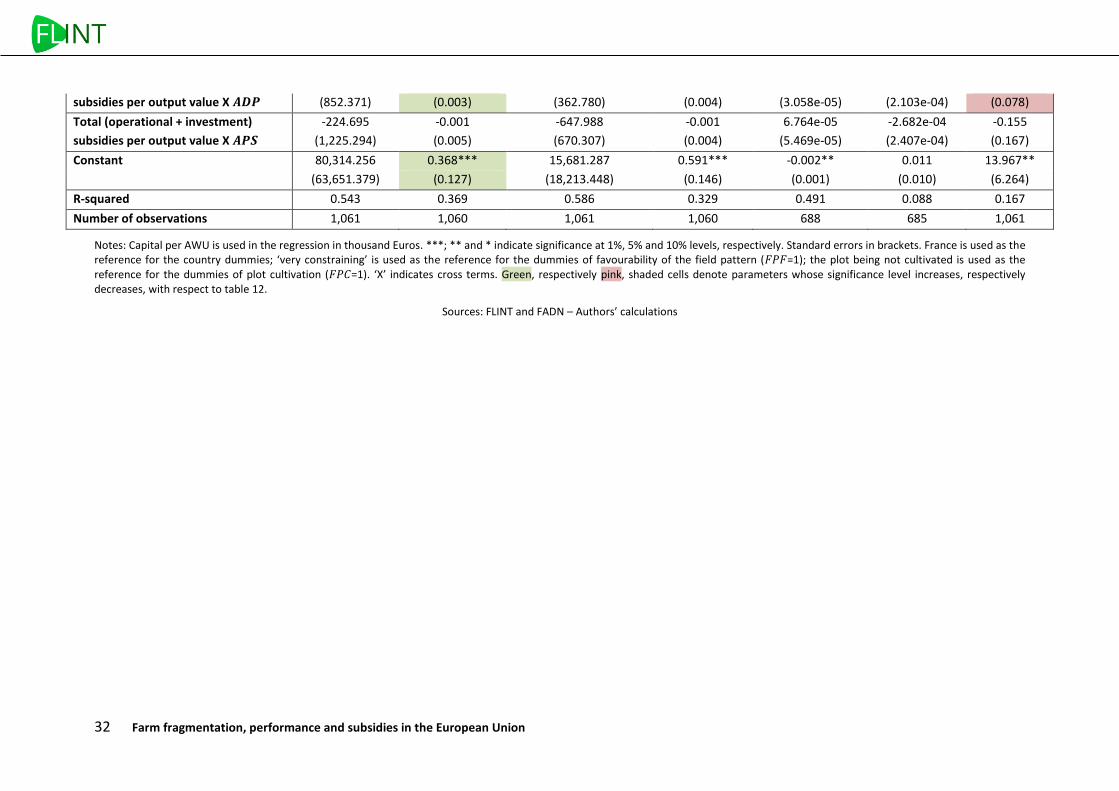
32 Farm fragmentation, performance and subsidies in the European Union
subsidies per output value X 𝑨𝑫𝑷 (852.371) (0.003) (362.780) (0.004) (3.058e-05) (2.103e-04) (0.078)
Total (operational + investment) -224.695 -0.001 -647.988 -0.001 6.764e-05 -2.682e-04 -0.155
subsidies per output value X 𝑨𝑷𝑺 (1,225.294) (0.005) (670.307) (0.004) (5.469e-05) (2.407e-04) (0.167)
Constant 80,314.256 0.368*** 15,681.287 0.591*** -0.002** 0.011 13.967**
(63,651.379) (0.127) (18,213.448) (0.146) (0.001) (0.010) (6.264)
R-squared 0.543 0.369 0.586 0.329 0.491 0.088 0.167
Number of observations 1,061 1,060 1,061 1,060 688 685 1,061
Notes: Capital per AWU is used in the regression in thousand Euros. ***; ** and * indicate significance at 1%, 5% and 10% levels, respectively. Standard errors in brackets. France is used as the reference for the country dummies; ‘very constraining’ is used as the reference for the dummies of favourability of the field pattern (𝐹𝑃𝐹=1); the plot being not cultivated is used as the reference for the dummies of plot cultivation (𝐹𝑃𝐶=1). ‘X’ indicates cross terms. Green, respectively pink, shaded cells denote parameters whose significance level increases, respectively decreases, with respect to table 12.
Sources: FLINT and FADN – Authors’ calculations
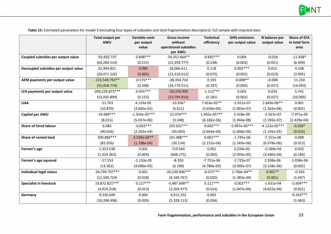
Farm fragmentation, performance and subsidies in the European Union 33
Table 15: Estimated parameters for model 3 (including four types of subsidies and land fragmentation descriptors): full sample with imputed data
Total output per AWU
Variable costs per output
value
Gross income without
operational subsidies per AWU
Technical efficiency
GHG emissions per output value
N balance per output value
Share of EFA in total farm
area
Coupled subsidies per output value -92,692.737 0.848*** -54,352.664** -0.692*** 0.004 -0.018 -11.838*
(64,284.514) (0.221) (22,359.777) (0.238) (0.003) (0.021) (6.499)
Decoupled subsidies per output value 32,994.821 0.095 18,066.611 0.118 0.005*** 0.015 4.548
(20,471.226) (0.065) (12,318.012) (0.075) (0.001) (0.013) (3.995)
AEM payments per output value -123,549.793** -0.576*** -38,350.710 0.193 -0.008** -0.008 11.234
(55,458.770) (0.208) (34,774.511) (0.297) (0.004) (0.027) (14.093)
LFA payments per output value -209,239.873*** 0.455*** -34,376.909 -1.112*** 0.003 0.024 5.741
(53,435.899) (0.153) (23,794.913) (0.181) (0.002) (0.027) (10.005)
UAA -11.763 4.133e-05 -10.936* 7.453e-05** -2.921e-07 2.843e-06** 0.001
(10.870) (3.665e-05) (5.611) (3.650e-05) (1.893e-07) (1.362e-06) (0.001)
Capital per AWU 43.689*** -1.334e-05*** 22.974*** 1.992e-05*** 5.418e-09 -2.567e-07 -7.971e-05
(8.015) (5.037e-06) (3.248) (6.182e-06) (1.944e-08) (1.593e-07) (2.429e-04)
Share of hired labour 6.083 -0.002*** 193.031*** 0.002*** -5.997e-06*** -4.122e-05*** -0.028*
(90.026) (2.262e-04) (45.043) (2.664e-04) (1.846e-06) (1.191e-05) (0.016)
Share of rented land 300.884*** 4.539e-04** 101.488*** 0.001*** -1.745e-06 -7.151e-06 0.008
(81.056) (1.798e-04) (30.134) (2.152e-04) (1.343e-06) (6.978e-06) (0.013)
Farmer’s age 1,353.538 0.001 719.564 0.001 3.234e-05 -3.189e-04 0.032
(1,324.363) (0.004) (608.275) (0.005) (2.993e-05) (3.440e-04) (0.184)
Farmer’s age squared -17.553 -1.133e-05 -8.350 -7.751e-06 -2.725e-07 2.938e-06 -1.038e-04
(13.362) (4.090e-05) (6.199) (4.780e-05) (3.095e-07) (3.158e-06) (0.002)
Individual legal status -34,799.707*** 0.001 -20,239.906*** -0.072*** 2.790e-04** 0.001** -0.350
(11,500.724) (0.018) (4,169.767) (0.020) (1.383e-04) (0.001) (1.047)
Specialist in livestock 19,872.821*** 0.117*** -5,487.668** 0.111*** 0.002*** -1.631e-04 -2.604***
(4,924.318) (0.013) (2,204.477) (0.014) (1.047e-04) (4.822e-04) (0.851)
Germany 9,336.649 0.004 4,913.102 0.002 -9.243***
(10,398.498) (0.029) (5,328.113) (0.036) (1.463)
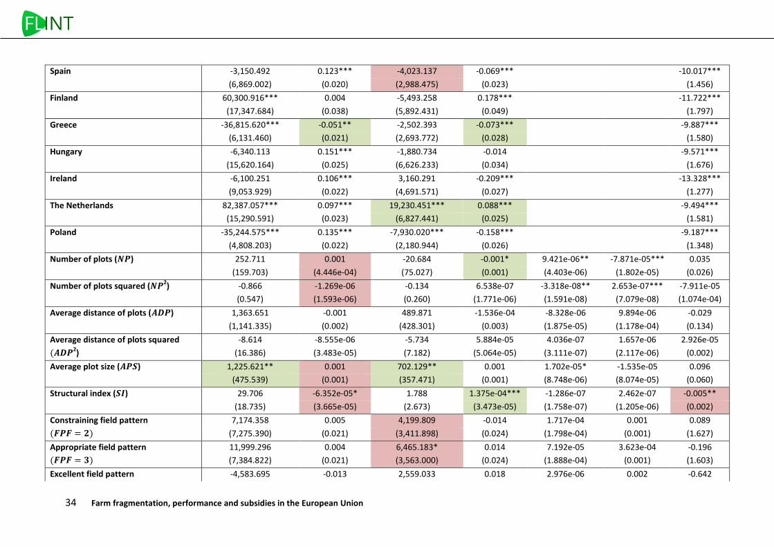
34 Farm fragmentation, performance and subsidies in the European Union
Spain -3,150.492 0.123*** -4,023.137 -0.069*** -10.017***
(6,869.002) (0.020) (2,988.475) (0.023) (1.456)
Finland 60,300.916*** 0.004 -5,493.258 0.178*** -11.722***
(17,347.684) (0.038) (5,892.431) (0.049) (1.797)
Greece -36,815.620*** -0.051** -2,502.393 -0.073*** -9.887***
(6,131.460) (0.021) (2,693.772) (0.028) (1.580)
Hungary -6,340.113 0.151*** -1,880.734 -0.014 -9.571***
(15,620.164) (0.025) (6,626.233) (0.034) (1.676)
Ireland -6,100.251 0.106*** 3,160.291 -0.209*** -13.328***
(9,053.929) (0.022) (4,691.571) (0.027) (1.277)
The Netherlands 82,387.057*** 0.097*** 19,230.451*** 0.088*** -9.494***
(15,290.591) (0.023) (6,827.441) (0.025) (1.581)
Poland -35,244.575*** 0.135*** -7,930.020*** -0.158*** -9.187***
(4,808.203) (0.022) (2,180.944) (0.026) (1.348)
Number of plots (𝑵𝑷) 252.711 0.001 -20.684 -0.001* 9.421e-06** -7.871e-05*** 0.035
(159.703) (4.446e-04) (75.027) (0.001) (4.403e-06) (1.802e-05) (0.026)
Number of plots squared (𝑵𝑷2) -0.866 -1.269e-06 -0.134 6.538e-07 -3.318e-08** 2.653e-07*** -7.911e-05
(0.547) (1.593e-06) (0.260) (1.771e-06) (1.591e-08) (7.079e-08) (1.074e-04)
Average distance of plots (𝑨𝑫𝑷) 1,363.651 -0.001 489.871 -1.536e-04 -8.328e-06 9.894e-06 -0.029
(1,141.335) (0.002) (428.301) (0.003) (1.875e-05) (1.178e-04) (0.134)
Average distance of plots squared -8.614 -8.555e-06 -5.734 5.884e-05 4.036e-07 1.657e-06 2.926e-05
(𝑨𝑫𝑷2)
(16.386) (3.483e-05) (7.182) (5.064e-05) (3.111e-07) (2.117e-06) (0.002)
Average plot size (𝑨𝑷𝑺) 1,225.621** 0.001 702.129** 0.001 1.702e-05* -1.535e-05 0.096
(475.539) (0.001) (357.471) (0.001) (8.748e-06) (8.074e-05) (0.060)
Structural index (𝑺𝑰) 29.706 -6.352e-05* 1.788 1.375e-04*** -1.286e-07 2.462e-07 -0.005**
(18.735) (3.665e-05) (2.673) (3.473e-05) (1.758e-07) (1.205e-06) (0.002)
Constraining field pattern 7,174.358 0.005 4,199.809 -0.014 1.717e-04 0.001 0.089
(𝑭𝑷𝑭 = 𝟐) (7,275.390) (0.021) (3,411.898) (0.024) (1.798e-04) (0.001) (1.627)
Appropriate field pattern 11,999.296 0.004 6,465.183* 0.014 7.192e-05 3.623e-04 -0.196
(𝑭𝑷𝑭 = 𝟑) (7,384.822) (0.021) (3,563.000) (0.024) (1.888e-04) (0.001) (1.603)
Excellent field pattern -4,583.695 -0.013 2,559.033 0.018 2.976e-06 0.002 -0.642
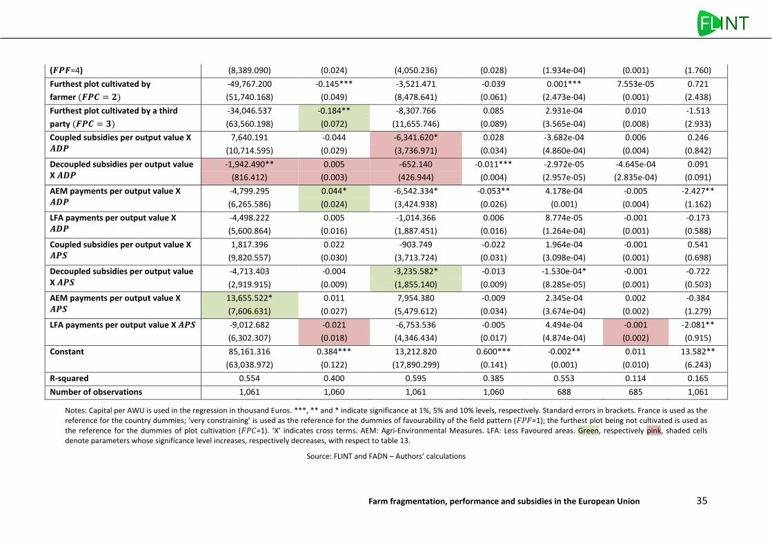
Farm fragmentation, performance and subsidies in the European Union 35
(𝑭𝑷𝑭=4) (8,389.090) (0.024) (4,050.236) (0.028) (1.934e-04) (0.001) (1.760)
Furthest plot cultivated by -49,767.200 -0.145*** -3,521.471 -0.039 0.001*** 7.553e-05 0.721
farmer (𝑭𝑷𝑪 = 𝟐) (51,740.168) (0.049) (8,478.641) (0.061) (2.473e-04) (0.001) (2.438)
Furthest plot cultivated by a third -34,046.537 -0.184** -8,307.766 0.085 2.931e-04 0.010 -1.513
party (𝑭𝑷𝑪 = 𝟑) (63,560.198) (0.072) (11,655.746) (0.089) (3.565e-04) (0.008) (2.933)
Coupled subsidies per output value X 𝑨𝑫𝑷
7,640.191 -0.044 -6,341.620* 0.028 -3.682e-04 0.006 0.246
(10,714.595) (0.029) (3,736.971) (0.034) (4.860e-04) (0.004) (0.842)
Decoupled subsidies per output value X 𝑨𝑫𝑷
-1,942.490** 0.005 -652.140 -0.011*** -2.972e-05 -4.645e-04 0.091
(816.412) (0.003) (426.944) (0.004) (2.957e-05) (2.835e-04) (0.091)
AEM payments per output value X 𝑨𝑫𝑷
-4,799.295 0.044* -6,542.334* -0.053** 4.178e-04 -0.005 -2.427**
(6,265.586) (0.024) (3,424.938) (0.026) (0.001) (0.004) (1.162)
LFA payments per output value X 𝑨𝑫𝑷
-4,498.222 0.005 -1,014.366 0.006 8.774e-05 -0.001 -0.173
(5,600.864) (0.016) (1,887.451) (0.016) (1.264e-04) (0.001) (0.588)
Coupled subsidies per output value X 𝑨𝑷𝑺
1,817.396 0.022 -903.749 -0.022 1.964e-04 -0.001 0.541
(9,820.557) (0.030) (3,713.724) (0.031) (3.098e-04) (0.001) (0.698)
Decoupled subsidies per output value X 𝑨𝑷𝑺
-4,713.403 -0.004 -3,235.582* -0.013 -1.530e-04* -0.001 -0.722
(2,919.915) (0.009) (1,855.140) (0.009) (8.285e-05) (0.001) (0.503)
AEM payments per output value X 𝑨𝑷𝑺
13,655.522* 0.011 7,954.380 -0.009 2.345e-04 0.002 -0.384
(7,606.631) (0.027) (5,479.612) (0.034) (3.674e-04) (0.002) (1.279)
LFA payments per output value X 𝑨𝑷𝑺 -9,012.682 -0.021 -6,753.536 -0.005 4.494e-04 -0.001 -2.081**
(6,302.307) (0.018) (4,346.434) (0.017) (4.874e-04) (0.002) (0.915)
Constant 85,161.316 0.384*** 13,212.820 0.600*** -0.002** 0.011 13.582**
(63,038.972) (0.122) (17,890.299) (0.141) (0.001) (0.010) (6.243)
R-squared 0.554 0.400 0.595 0.385 0.553 0.114 0.165
Number of observations 1,061 1,060 1,061 1,060 688 685 1,061
Notes: Capital per AWU is used in the regression in thousand Euros. ***, ** and * indicate significance at 1%, 5% and 10% levels, respectively. Standard errors in brackets. France is used as the reference for the country dummies; ‘very constraining’ is used as the reference for the dummies of favourability of the field pattern (𝐹𝑃𝐹=1); the furthest plot being not cultivated is used as the reference for the dummies of plot cultivation (𝐹𝑃𝐶=1). ‘X’ indicates cross terms. AEM: Agri-Environmental Measures. LFA: Less Favoured areas. Green, respectively pink, shaded cells denote parameters whose significance level increases, respectively decreases, with respect to table 13.
Source: FLINT and FADN – Authors’ calculations

36 Farm fragmentation, performance and subsidies in the European Union
4 CONCLUSION Land fragmentation of the field pattern is a structural characteristic of holdings which has to be taken into account when investigating the drivers of farm performance. Difference in LF may indeed be a source of difference in productivity or efficiency among farms which may appear as equivalent on other grounds. Not taking LF into account would lead to spuriously attribute its impact either to the farmers’ ability or to other variables of interest such as public support.
However, as previous studies have shown, it has been difficult to take LF into account in a satisfactory way so far because no consistent database exists which gathers for the same farms and at the same time both performance- and LF-related variables and indicators. It was one objective of the FLINT project to fill this gap and to provide such consistent data in an operational and tractable way for a sample of more than 1,000 farms in 9 EU countries. The small set of LF-related variables surveyed in the FLINT project may look simplified with respect to the precise information which could be obtained from other specific databases such as the national LPIS. Together with the information regarding the farm’s UAA already available in the FADN, they nonetheless allow deriving effective LF indicators.
The analysis proposed here leads to draw several conclusions. Firstly, there exists a wide variety of situations with respect to farm LF across EU Member States and farming specialisations. Secondly, LF seems to be only loosely related to working conditions and quality of life indicators for the studied sample. Thirdly, taking LF into account does change the results obtained when analysing the links between agricultural subsidies and farm technical, economic and environmental performance. When subsidies are considered as a whole, most of their impact seems to come from the interaction with the average distance of farm plots, an effect which is not captured when LF is not taken into account. This seems to be also true as far as decoupled payments are concerned while the impacts of other types of subsidies appear to be more direct, i.e., disconnected from the level of LF. Lastly, the analysis also reveals that enlarging the studied sample by imputing data to replace missing values does not actually constitute an improvement as it may lead to degrade slightly the explanatory power of the model and blur the results regarding the relationships between the dependent variable and the chosen covariates. This strongly advocates for gathering data as exhaustively and precisely for the same farms and at the same time.
Finally, it should be noted that the present analysis is only an exploratory exercise. It nonetheless allowed to derive interesting results which would have to be further investigated on a larger sample and for several periods to be either confirmed or refined. Extending the observation basis both in its cross-section and longitudinal dimensions would also allow using more elaborate econometric techniques in order to account for well-known limitations such as potential endogeneity and panel-data variability.
Acknowledgements
The authors thank the FLINT partners for providing access to the data, to Yann Desjeux for helping in data processing and to Hervé Dakpo for technical efficiency calculation.
Farm fragmentation, performance and subsidies in the European Union 37
5 REFERENCES Blarel B., Hazell P., Place F., Quiggin J. (1992) The economics of farm fragmentation: Evidence from Ghana and Rwanda. The World Bank Economic Review, 6: 233-254.
Del Corral J., Perez J.A., Roibas D. (2011) The impact of land fragmentation on milk production. Journal of Dairy Science, 94: 517-525.
Di Falco S., Penov I., Aleksiev A., van Rensburg T. (2010) Agrobiodiversity, farm profits and land fragmentation: Evidence from Bulgaria. Land Use Policy, 27: 763-771.
Kawasaki, K. (2010) The costs and benefits of land fragmentation of rice farms in Japan. Australian Journal of Agricultural and Resource Economics, 54: 509-526.
Latruffe L., Piet L. (2014) Does land fragmentation affect farm performance? A case study from Brittany, France. Agricultural Systems, 129: 68-80.
Manjunatha A., Anik A.R., Speelman S. Nuppenau E. (2013) Impact of land fragmentation, farm size, land ownership and crop diversity on profit and efficiency of irrigated farms in India. Land Use Policy, 31: 397-405.
Marie M. (2009) Des pratiques des agriculteurs à la production de paysage de bocage. Etude comparée des dynamiques et des logiques d’organisation spatiale des systèmes agricoles laitiers en Europe, Basse-Normandie, Galice, Sud de l’Angleterre. Ph-D dissertation of the University of Caen/Basse-Normandie, Caen (France).
Renard M. (1972) Recherches méthodologiques sur le degré d’émiettement parcellaire des exploitations agricoles des bocages de l’ouest. Bulletin de l'Association de Géographes Français, 49(397): 83-94.