StanStatistical Inference Made Easy

Core Development Team (20 people, ∼4 FTE)

Andrew Gelman, Bob Carpenter, Matt Hoffman, Daniel Lee,

Ben Goodrich, Michael Betancourt, Marcus Brubaker, Jiqiang Guo,

Peter Li, Allen Riddell, Marco Inacio, Jeffrey Arnold,

Mitzi Morris, Rob Trangucci, Rob Goedman, Brian Lau,

Jonah Sol Gabray, Alp Kucukelbir, Robert L. Grant, Dustin Tran

Stan 2.7.0 (July 2015) http://mc-stan.org

1

Section 1.

Bayesian Inference

Bob Carpenter

Columbia University

2

Warmup Exercise I

Sample Variation

3

Repeated i.i.d. Trials

• Suppose we repeatedly generate a ran-dom outcome from among several po-tential outcomes

• Suppose the outcome chances are thesame each time

– i.e., outcomes are independent andidentically distributed (i.i.d.)

• For example, spin a fair spinner (with-out cheating), such as one from FamilyCricket.

Image source: http://replaycricket.com/2010/10/29/family-cricket/

4

Repeated i.i.d. Binary Trials

• Suppose the outcome is binary and assigned to 0 or 1;e.g.,

– 20% chance of outcome 1: ball in play

– 80% chance of outcome 0: ball not in play

• Consider different numbers of bowls delivered.

• How will proportion of successes in sample differ?

5

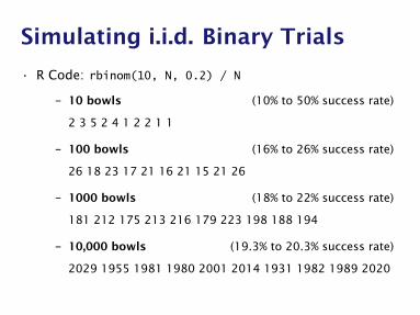
Simulating i.i.d. Binary Trials

• R Code: rbinom(10, N, 0.2) / N

– 10 bowls (10% to 50% success rate)

2 3 5 2 4 1 2 2 1 1

– 100 bowls (16% to 26% success rate)

26 18 23 17 21 16 21 15 21 26

– 1000 bowls (18% to 22% success rate)

181 212 175 213 216 179 223 198 188 194

– 10,000 bowls (19.3% to 20.3% success rate)

2029 1955 1981 1980 2001 2014 1931 1982 1989 2020

6

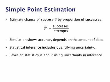
Simple Point Estimation

• Estimate chance of success θ by proportion of successes:

θ∗ = successesattempts

• Simulation shows accuracy depends on the amount of data.

• Statistical inference includes quantifying uncertainty.

• Bayesian statistics is about using uncertainty in inference.

7

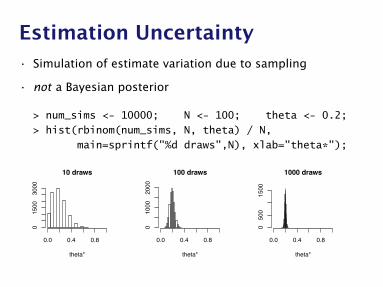
Estimation Uncertainty• Simulation of estimate variation due to sampling

• not a Bayesian posterior

> num_sims <- 10000; N <- 100; theta <- 0.2;

> hist(rbinom(num_sims, N, theta) / N,

main=sprintf("%d draws",N), xlab="theta*");

Confidence via Simulation

• P% confidence interval: interval in which P% of the esti-mates are expected to fall.

• Simulation computes intervals to any accuracy.

• Simulate, sort, and inspect the central empirical interval.

10 draws

theta*

0.0 0.4 0.8

01500

3000

100 draws

theta*

0.0 0.4 0.8

01000

2000

1000 draws

theta*

0.0 0.4 0.8

0500

1500

• Estimator uncertainty, not a Bayesian posterior

8

8

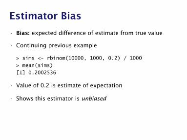
Estimator Bias

• Bias: expected difference of estimate from true value

• Continuing previous example

> sims <- rbinom(10000, 1000, 0.2) / 1000

> mean(sims)

[1] 0.2002536

• Value of 0.2 is estimate of expectation

• Shows this estimator is unbiased

9

Simple Point Estimation (cont.)

• Central Limit Theorem: expected error in θ∗ goes down

as1√N

• Each decimal place of accuracy requires 100× more sam-ples.

• Width of confidence intervals shrinks at the same rate.

• Can also use theory to show this estimator is unbiased.

10

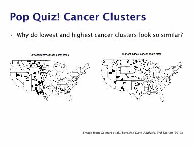
Pop Quiz! Cancer Clusters

• Why do lowest and highest cancer clusters look so similar?

Image from Gelman et al., Bayesian Data Analysis, 3rd Edition (2013)

11

Pop Quiz Answer

• Hint: mix earlier simulations of repeated i.i.d. trials with20% success and sort:

1/10 1/10 1/10 15/100 16/10017/100 175/1000 179/1000 18/100 181/1000

188/1000 194/1000 198/1000 2/10 2/102/10 2/10 21/100 21/100 21/100

212/1000 213/1000 216/1000 223/1000 23/10026/100 26/100 3/10 4/10 5/10

• More variation in observed rates with smaller sample sizes

• Answer: High cancer and low cancer counties are smallpopulations

12

Warmup Exercise II

Maximum LikelihoodEstimation

13

Observations, Counterfactuals,and Random Variables

• Assume we observe data y = y1, . . . , yN

• Statistical modeling assumes even though y is observed,the values could have been different

• John Stuart Mill first characterized this counterfactual na-ture of statistical modeling in:

A System of Logic, Ratiocinative and Inductive (1843)

• In measure-theoretic language, y is a random variable

14

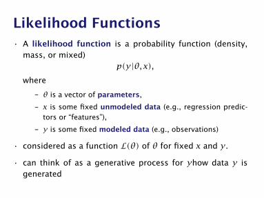
Likelihood Functions• A likelihood function is a probability function (density,

mass, or mixed)p(y|θ, x),

where

– θ is a vector of parameters,

– x is some fixed unmodeled data (e.g., regression predic-tors or “features”),

– y is some fixed modeled data (e.g., observations)

• considered as a function L(θ) of θ for fixed x and y.

• can think of as a generative process for yhow data y isgenerated

15

Maximum Likelihood Estimation

• Estimate parameters θ given observations y.

• Maximum likelihood estimation (MLE) chooses estimatethat maximizes the likelihood function, i.e.,

θ∗ = arg maxθ L(θ) = arg maxθ p(y|θ, x)

• This function of L and y (and x) is called an estimator

16

Example of MLE• The frequency-based estimate

θ∗ = 1N

N∑n=1yn,

is the observed rate of “success” (outcome 1) observations.

• This is the MLE for the model

p(y|θ) =N∏n=1p(yn|θ) =

N∏n=1

Bernoulli(yn|θ)

where for u ∈ {0,1},

Bernoulli(u|θ) =

θ if u = 11− θ if u = 0

17

Example of MLE (cont.)

• First modeling assumption is that data are i.i.d.,

p(y|θ) =N∏n=1p(yn|θ)

• Second modeling assumption is form of likelihood,

p(yn|θ) = Bernoulli(yn|θ)

18

Example of MLE (cont.)

• The frequency-based estimate is the MLE

• First derivative is zero (indicating min or max),

L′y(θ∗) = 0,

• Second derivative is negative (indicating max),

L′′y (θ∗) < 0.

19

MLEs can be Dangerous!

• Recall the cancer cluster example

• Accuracy is low with small counts

• What we need are hierarchical models (stay tuned)

20

Part I

Bayesian Inference

21

Bayesian Data Analysis

• “By Bayesian data analysis, we mean practical methods formaking inferences from data using probability models forquantities we observe and about which we wish to learn.”

• “The essential characteristic of Bayesian methods is theirexplict use of probability for quantifying uncertainty ininferences based on statistical analysis.”

Gelman et al., Bayesian Data Analysis, 3rd edition, 2013

22

Bayesian Methodology• Set up full probability model

– for all observable & unobservable quantities

– consistent w. problem knowledge & data collection

• Condition on observed data

– to caclulate posterior probability of unobserved quan-tities (e.g., parameters, predictions, missing data)

• Evaluate

– model fit and implications of posterior

• Repeat as necessary

Ibid.

23

Where do Models Come from?

• Sometimes model comes first, based on substantive con-siderations

– toxicology, economics, ecology, . . .

• Sometimes model chosen based on data collection

– traditional statistics of surveys and experiments

• Other times the data comes first

– observational studies, meta-analysis, . . .

• Usually its a mix

24

(Donald) Rubin’s Philosophy

• All statistics is inference about missing data

• Question 1: What would you do if you had all the data?

• Question 2: What were you doing before you had any data?

(as relayed in course notes by Andrew Gelman)

25

Model Checking• Do the inferences make sense?

– are parameter values consistent with model’s prior?

– does simulating from parameter values produce reasoablefake data?

– are marginal predictions consistent with the data?

• Do predictions and event probabilities for new data makesense?

• Not: Is the model true?

• Not: What is Pr[model is true]?

• Not: Can we “reject” the model?

26

Model Improvement

• Expanding the model

– hierarchical and multilevel structure . . .

– more flexible distributions (overdispersion, covariance)

– more structure (geospatial, time series)

– more modeling of measurement methods and errors

– . . .

• Including more data

– breadth (more predictors or kinds of observations)

– depth (more observations)

27

Using Bayesian Inference

• Finds parameters consistent with prior info and data∗

– ∗ if such agreement is possible

• Automatically includes uncertainty and variability

• Inferences can be plugged in directly

– risk assesment

– decision analysis

28

Notation for Basic Quantities

• Basic Quantities

– y: observed data

– θ: parameters (and other unobserved quantities)

– x: constants, predictors for conditional (aka “discrimina-tive”) models

• Basic Predictive Quantities

– y: unknown, potentially observable quantities

– x: constants, predictors for unknown quantities

29

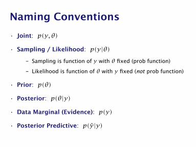
Naming Conventions

• Joint: p(y, θ)

• Sampling / Likelihood: p(y|θ)

– Sampling is function of y with θ fixed (prob function)

– Likelihood is function of θ with y fixed (not prob function)

• Prior: p(θ)

• Posterior: p(θ|y)

• Data Marginal (Evidence): p(y)

• Posterior Predictive: p(y|y)

30

Bayes’s Rule for Posterior

p(θ|y) = p(y, θ)p(y)

[def of conditional]

= p(y|θ)p(θ)p(y)

[chain rule]

= p(y|θ)p(θ)∫Θ p(y, θ′) dθ′

[law of total prob]

= p(y|θ)p(θ)∫Θ p(y|θ′)p(θ′) dθ′

[chain rule]

• Inversion: Final result depends only on sampling distribu-tion (likelihood) p(y|θ) and prior p(θ)

31

Bayes’s Rule up to Proportion

• If data y is fixed, then

p(θ|y) = p(y|θ)p(θ)p(y)

∝ p(y|θ)p(θ)

= p(y, θ)

• Posterior proportional to likelihood times prior

• Equivalently, posterior proportional to joint

• The nasty integral for data marginal p(y) goes away

32

Posterior Predictive Distribution

• Predict new data y based on observed data y

• Marginalize out parameters from posterior

p(y|y) =∫Θp(y|θ)p(θ|y)dθ.

• Averages predictions p(y|θ), weight by posterior p(θ|y)

– Θ = {θ | p(θ|y) > 0} is support of p(θ|y)

• Allows continuous, discrete, or mixed parameters

– integral notation shorthand for sums and/or integrals

33

Event Probabilities• Recall that an event A is a collection of outcomes

• Suppose event A is determined by indicator on parameters

f (θ) =

1 if θ ∈ A0 if θ 6∈ A

• e.g., f (θ) = I(θ1 > θ2) for Pr[θ1 > θ2 |y]

• Bayesian event probabilities calculate posterior mass

Pr[A] =∫Θf (θ)p(θ|y)dθ.

• Not frequentist, because involves parameter probabilities

34

Example I

Male Birth Ratio

35

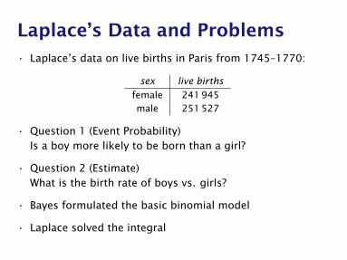
Laplace’s Data and Problems• Laplace’s data on live births in Paris from 1745–1770:

sex live births

female 241 945male 251 527

• Question 1 (Event Probability)Is a boy more likely to be born than a girl?

• Question 2 (Estimate)What is the birth rate of boys vs. girls?

• Bayes formulated the basic binomial model

• Laplace solved the integral

36

Binomial Distribution• Binomial distribution is number of successes y in N i.i.d.

Bernoulli trials with chance of success θ

• If y1, . . . , yN ∼ Bernoulli(θ),

then (y1 + · · · + yN) ∼ Binomial(N,θ)

• The analytic form is

Binomial(y|N,θ) =(Ny

)θy(1− θ)N−y

where the binomial coefficient normalizes for permuta-tions (i.e., which subset of n has yn = 1),(

Ny

)= N!y ! (N − y)!

37

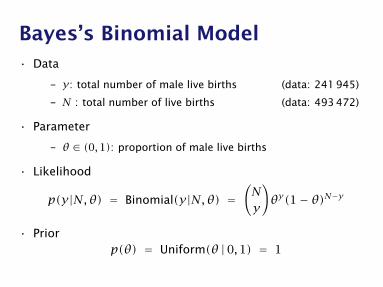
Bayes’s Binomial Model• Data

– y: total number of male live births (data: 241 945)

– N : total number of live births (data: 493 472)

• Parameter

– θ ∈ (0,1): proportion of male live births

• Likelihood

p(y|N,θ) = Binomial(y|N,θ) =(Ny

)θy(1− θ)N−y

• Priorp(θ) = Uniform(θ |0,1) = 1

38

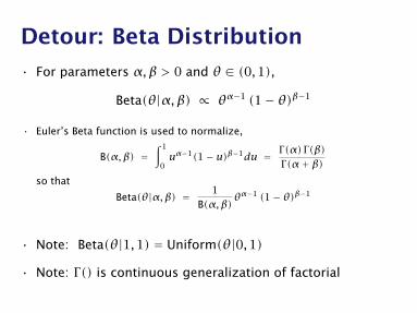
Detour: Beta Distribution

• For parameters α,β > 0 and θ ∈ (0,1),

Beta(θ|α,β) ∝ θα−1 (1− θ)β−1

• Euler’s Beta function is used to normalize,

B(α,β) =∫ 10uα−1(1− u)β−1du = Γ(α) Γ(β)

Γ(α+ β)so that

Beta(θ|α,β) = 1B(α,β)

θα−1 (1− θ)β−1

• Note: Beta(θ|1,1) = Uniform(θ|0,1)

• Note: Γ() is continuous generalization of factorial

39

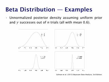
Beta Distribution — Examples• Unnormalized posterior density assuming uniform prior

and y successes out of n trials (all with mean 0.6).30 2. SINGLE-PARAMETER MODELS

Figure 2.1 Unnormalized posterior density for binomial parameter θ, based on uniform prior dis-tribution and y successes out of n trials. Curves displayed for several values of n and y.

(2.1), we are assuming that the n births are conditionally independent given θ, withthe probability of a female birth equal to θ for all cases. This modeling assumptionis motivated by the exchangeability that may be judged to arise when we have noexplanatory information (for example, distinguishing multiple births or births withinthe same family) that might affect the sex of the baby.

To perform Bayesian inference in the binomial model, we must specify a prior distribu-tion for θ. We will discuss issues associated with specifying prior distributions many timesthroughout this book, but for simplicity at this point, we assume that the prior distributionfor θ is uniform on the interval [0, 1].

Elementary application of Bayes’ rule as displayed in (1.2), applied to (2.1), then givesthe posterior density for θ as

p(θ|y) ∝ θy(1− θ)n−y. (2.2)

With fixed n and y, the factor!ny

"does not depend on the unknown parameter θ, and so it

can be treated as a constant when calculating the posterior distribution of θ. As is typicalof many examples, the posterior density can be written immediately in closed form, up to aconstant of proportionality. In single-parameter problems, this allows immediate graphicalpresentation of the posterior distribution. For example, in Figure 2.1, the unnormalizeddensity (2.2) is displayed for several different experiments, that is, different values of n andy. Each of the four experiments has the same proportion of successes, but the sample sizesvary. In the present case, we can recognize (2.2) as the unnormalized form of the betadistribution (see Appendix A),

θ|y ∼ Beta(y + 1, n− y + 1). (2.3)

Historical note: Bayes and LaplaceMany early writers on probability dealt with the elementary binomial model. The firstcontributions of lasting significance, in the 17th and early 18th centuries, concentratedon the ‘pre-data’ question: given θ, what are the probabilities of the various possibleoutcomes of the random variable y? For example, the ‘weak law of large numbers’ of

Gelman et al. (2013) Bayesian Data Analysis, 3rd Edition.

40

Laplace Turns the Crank

• From Bayes’s rule, the posterior is

p(θ|y,N) = Binomial(y|N,θ)Uniform(θ|0,1)∫Θ Binomial(y|N,θ′)p(θ′) dθ′

• Laplace calculated the posterior analytically

p(θ|y,N) = Beta(θ |y + 1, N − y + 1).

41

Estimation

• Posterior is Beta(θ |1+ 241945, 1+ 251527)

• Posterior mean:

1+ 2419451+ 241945+ 1+ 251527 ≈ 0.4902913

• Maximum likelihood estimate same as posterior mode (be-cause of uniform prior)

241945241945+ 251527 ≈ 0.4902912

• As number of observations approaches ∞,MLE approaches posterior mean

42

Event Probability Inference• What is probability that a male live birth is more likely than

a female live birth?

Pr[θ > 0.5] =∫Θ

I[θ > 0.5]p(θ|y,N)dθ

=∫ 10.5p(θ|y,N)dθ

= 1− Fθ|y,N(0.5)

≈ 10−42

• I[φ] = 1 if condition φ is true and 0 otherwise.

• Fθ|y,N is posterior cumulative distribution function (cdf).

43

Mathematics vs. Simulation

• Luckily, we don’t have to be as good at math as Laplace

• Nowadays, we calculate all these integrals by computerusing tools like Stan

If you wanted to do foundational research instatistics in the mid-twentieth century, you hadto be bit of a mathematician, whether you wantedto or not. . . . if you want to do statistical re-search at the turn of the twenty-first century,you have to be a computer programmer.

—from Andrew’s blog

44

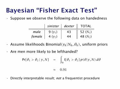
Bayesian “Fisher Exact Test”• Suppose we observe the following data on handedness

sinister dexter TOTAL

male 9 (y1) 43 52 (N1)female 4 (y2) 44 48 (N2)

• Assume likelihoods Binomial(yk|Nk, θk), uniform priors

• Are men more likely to be lefthanded?

Pr[θ1 > θ2 |y,N] =∫Θ

I[θ1 > θ2]p(θ|y,N)dθ

≈ 0.91

• Directly interpretable result; not a frequentist procedure

45

Visualizing Posterior Difference• Plot of posterior difference, p(θ1−θ2 |y,N) (men - women)

• Vertical bars: central 95% posterior interval (−0.05,0.22)

46

Technical Interlude

Conjugate Priors

47

Conjugate Priors

• Family F is a conjugate prior for family G if

– prior in F and

– likelihood in G,

– entails posterior in F

• Before MCMC techniques became practical, Bayesian anal-ysis mostly involved conjugate priors

• Still widely used because analytic solutions are more effi-cient than MCMC

48

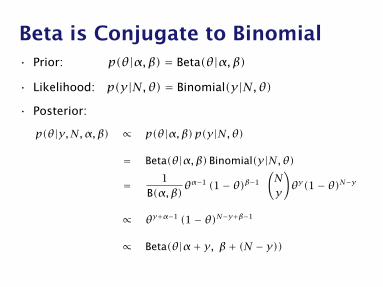
Beta is Conjugate to Binomial• Prior: p(θ|α,β) = Beta(θ|α,β)

• Likelihood: p(y|N,θ) = Binomial(y|N,θ)

• Posterior:

p(θ|y,N,α,β) ∝ p(θ|α,β)p(y|N,θ)

= Beta(θ|α,β)Binomial(y|N,θ)

= 1B(α,β)

θα−1 (1− θ)β−1(Ny

)θy(1− θ)N−y

∝ θy+α−1 (1− θ)N−y+β−1

∝ Beta(θ|α+ y, β+ (N − y))

49

Chaining Updates• Start with prior Beta(θ|α,β)

• Receive binomial data in K statges (y1, N1), . . . , (yK , NK)

• After (y1, N1), posterior is Beta(θ|α+ y1, β+N1 − y1)

• Use as prior for (y2, N2), with posterior

Beta(θ|α+ y1 + y2, β+ (N1 − y1)+ (N2 − y2))

• Lather, rinse, repeat, until final posterior

Beta(θ|α+y1+· · ·+yK , β+(N1+· · ·+NK)−(y1+· · ·+yK))

• Same result as if we’d updated with combined data

Beta(y1 + · · · + yK , N1 + · · · +NK)

50

Part II

(Un-)BayesianPoint Estimation

51

MAP Estimator• For a Bayesian model p(y, θ) = p(y|θ)p(θ), the max a

posteriori (MAP) estimate maximizes the posterior,

θ∗ = arg maxθ p(θ|y)

= arg maxθp(y|θ)p(θ)p(y)

= arg maxθ p(y|θ)p(θ).

= arg maxθ logp(y|θ)+ logp(θ).

• not Bayesian because it doesn’t integrate over uncertainty

• not frequentist because of distributions over parameters

52

MAP and the MLE

• MAP estimate reduces to the MLE if the prior is uniform,i.e.,

p(θ) = c

because

θ∗ = arg maxθ p(y|θ)p(θ)

= arg maxθ p(y|θ) c

= arg maxθ p(y|θ).

53

Penalized Maximum Likelihood• The MAP estimate can be made palatable to frequentists

via philosophical sleight of hand

• Treat the negative log prior − logp(θ) as a “penalty”

• e.g., a Normal(θ|µ,σ) prior becomes a penalty function

λθ,µ,σ = −(

logσ + 12

(θ − µσ

)2)

• Maximize sum of log likelihood and negative penalty

θ∗ = arg maxθ logp(y|θ, x)− λθ,µ,σ

= arg maxθ logp(y|θ, x)+ logp(θ|µ,σ)

54

Proper Bayesian Point Estimates

• Choose estimate to minimize some loss function

• To minimize expected squared error (L2 loss), E[(θ−θ′)2 |y],use the posterior mean

θ = arg minθ′E[(θ − θ′)2 |y] =∫Θθ × p(θ|y)dθ.

• To minimize expected absolute error (L1 loss), E[|θ−θ′|],use the posterior median.

• Other loss (utility) functions possible, the study of whichfalls under decision theory

• All share property of involving full Bayesian inference.

55

Point Estimates for Inference?

• Common in machine learning to generate a point estimateθ∗, then use it for inference, p(y|θ∗)

• This is defective because it

underestimates uncertainty.

• To properly estimate uncertainty, apply full Bayes

• A major focus of statistics and decision theory is estimat-ing uncertainty in our inferences

56

Philosophical Interlude

What is Statistics?

57

Exchangeability

• Roughly, an exchangeable probability function is such thatfor a sequence of random variables y = y1, . . . , yN ,

p(y) = p(π(y))

for every N-permutation π (i.e, a one-to-one mapping of{1, . . . ,N})

• i.i.d. implies exchangeability, but not vice-versa

58

Exchangeability Assumptions

• Models almost always make some kind of exchangeabilityassumption

• Typically when other knowledge is not available

– e.g., treat voters as conditionally i.i.d. given their age, sex,income, education level, religous affiliation, and state ofresidence

– But voters have many more properties (hair color, height,profession, employment status, marital status, car owner-ship, gun ownership, etc.)

– Missing predictors introduce additional error (on top ofmeasurement error)

59

Random Parameters:Doxastic or Epistemic?• Bayesians treat distributions over parameters as epistemic

(i.e., about knowledge)

• They do not treat them as being doxastic(i.e., about beliefs)

• Priors encode our knowledge before seeing the data

• Posteriors encode our knowledge after seeing the data

• Bayes’s rule provides the way to update our knowledge

• People like to pretend models are ontological(i.e., about what exists)

60

Arbitrariness:Priors vs. Likelihood

• Bayesian analyses often criticized as subjective (arbitrary)

• Choosing priors is no more arbitrary than choosing a like-lihood function (or an exchangeability/i.i.d. assumption)

• As George Box famously wrote (1987),

“All models are wrong, but some are useful.”

• This does not just apply to Bayesian models!

61

Part IV

Hierarchical Models

62

Baseball At-Bats

• For example, consider baseball batting ability.

– Baseball is sort of like cricket, but with round bats, a one-way field,

stationary “bowlers”, four bases, short games, and no draws

• Batters have a number of “at-bats” in a season, out ofwhich they get a number of “hits” (hits are a good thing)

• Nobody with higher than 40% success rate since 1950s.

• No player (excluding “bowlers”) bats much less than 20%.

• Same approach applies to hospital pediatric surgery com-plications (a BUGS example), reviews on Yelp, test scoresin multiple classrooms, . . .

63

Baseball Data• Hits versus at bats for the

2006 American Leagueseason

• Not much variation inability!

• Ignore skill vs. at-bats re-lation

• Note uncertainty of MLE●●

●

●

●

●

●

●

●

●

●

●

●

●

●

● ●

●

●

●

●

●

●●

●

●

●

● ●

●

●

●

●

●

●

●

●

●●

● ●

●

●

●

●

●

●

●

●

●

● ●

●●

●

●

●

●

●

●

●

●

●

●

●

● ●

●

●

●

●

●

●

●

●

●●

●

●

●

●

●

●●

●

●●

● ●

●

●

●

●

●

●●

●

●●

●

●

●

●

●

●

●

●

●

●

●

●

●

●

●

●● ●

●

●

●●

●

●

●●

●

●

●

●

●

●

●

●●

●

●

●

● ●

●

●

●

●

●

●

●

●

●

●

●

●

●

●●

●

●

●●

●●

●

●

●

●

●

●

●●●

●

●

●●

●

●

●

●

●

●

●

●

●

●

●

●

●

●

●

● ●

●

●

●

●

●●

●

●

● ●

●

●

●

●

●

●

●

●

●

●

●

●

●

●

●

●

●

●

●

●

●●

●

●

●●

●●

●

●

●

●

●

●●

●

●

●

●

●

●

●

●

●●

●

●

● ●●●

●

●

●

●

●

●

●

●

●

●

●●●

●

●

●

●

●

●●

●

●●

●

●●

● ●

●

●

●

●

●

●●●●

●

●●

●●

●

●

●

●

●

●●

●

●●

●

●

●

●

●

at bats

avg

= h

its /

at b

ats

0.0

0.1

0.2

0.3

0.4

0.5

0.6

1 5 10 50 100 500

64

Pooling Data• How do we estimate the ability of a player who we observe

getting 6 hits in 10 at-bats? Or 0 hits in 5 at-bats? Esti-mates of 60% or 0% are absurd!

• Same logic applies to players with 152 hits in 537 at bats.

• No pooling: estimate each player separately

• Complete pooling: estimate all players together (assumeno difference in abilities)

• Partial pooling: somewhere in the middle

– use information about other players (i.e., the population)to estimate a player’s ability

65

Hierarchical Models

• Hierarchical models are principled way of determining howmuch pooling to apply.

• Pull estimates toward the population mean based on amountof variation in population

– low variance population: more pooling

– high variance population: less pooling

• In limit

– as variance goes to 0, get complete pooling

– as variance goes to ∞, get no pooling

66

Hierarchical Batting Ability

• Instead of fixed priors, estimate priors along with otherparameters

• Still only uses data once for a single model fit

• Data: yn, Bn: hits, at-bats for player n

• Parameters: θn: ability for player n

• Hyperparameters: α,β: population mean and variance

• Hyperpriors: fixed priors on α and β (hardcoded)

67

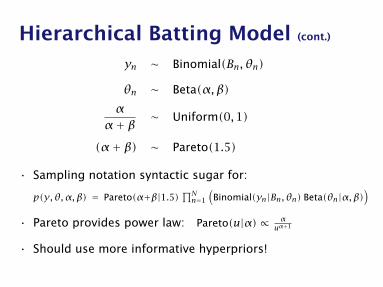
Hierarchical Batting Model (cont.)

yn ∼ Binomial(Bn, θn)

θn ∼ Beta(α,β)α

α+ β ∼ Uniform(0,1)

(α+ β) ∼ Pareto(1.5)

• Sampling notation syntactic sugar for:

p(y, θ,α,β) = Pareto(α+β|1.5)∏Nn=1

(Binomial(yn|Bn, θn) Beta(θn|α,β)

)• Pareto provides power law: Pareto(u|α)∝ α

uα+1

• Should use more informative hyperpriors!

68

Hierarchical Prior Posterior

• Draws from posterior(crosshairs at posteriormean)

• Prior population mean: 0.271

• Prior population scale: 400

• Together yield prior std devof 0.022

• Mean is better estimatedthan scale (typical)

69

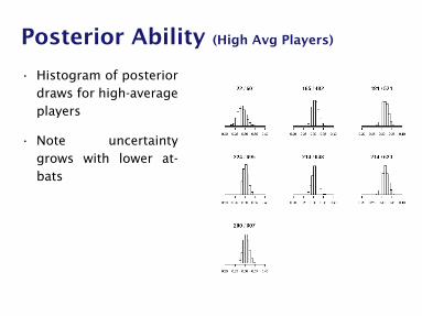
Posterior Ability (High Avg Players)

• Histogram of posteriordraws for high-averageplayers

• Note uncertaintygrows with lower at-bats

70

Multiple Comparisons• Who has the highest ability (based on this data)?

• Probabilty player n is best is

Average At-Bats Pr[best].347 521 0.12.343 623 0.11.342 482 0.08.330 648 0.04.330 607 0.04.367 60 0.02.322 695 0.02

• No clear winner—sample size matters.

• In last game (of 162), Mauer (Minnesota) edged out Jeter (NY)

71

End (Section 1)

72