standard error estimation for eu-silc target indicators...
TRANSCRIPT
Standard Error Estimation for EU-SILC target indica tors – First Results of the Net-SILC2 Project
Emilio Di Meglio1, Guillaume Osier2, Yves Berger3, Tim Goedemé4, and Emanuela
Di Falco5
1Eurostat, Unit F4 « Quality of Life », e-mail: [email protected]
2Statistics Luxembourg (STATEC) and Luxembourg Income Study, e-mail: [email protected]
3University of Southampton, UK, e-mail: [email protected]
4University of Antwerp, Belgium, e-mail: [email protected]
5Eurostat, Unit F4 « Quality of Life », e-mail: [email protected]
Abstract We present the first results of the Net-SILC2 project with regard to standard error estimation in
EU-SILC (EU Statistics on Income and Living Conditions). EU-SILC is the main data source for
comparative analysis and indicators on income and living conditions in the European Union
(EU), covering all the 27 EU countries and a number of other European countries. The growing
complexity of EU-SILC, the widening of the user community and the increasing reliance on EU-
SILC for policy targeting and evaluation have enhanced the need for comparable, accurate as
well as workable solutions to the estimation of standard errors and confidence intervals for the
indicators based on the EU-SILC surveys. After presenting the Net-SILC2 project and the
recommended variance estimators, we show preliminary estimates of standard error and
confidence intervals for cross-sectional measures, longitudinal measures and measures of changes
between two waves. The proposed approach is general and can be implemented with multistage
surveys. As far as variance of change is concerned, the proposed approach can be used with
rotating longitudinal surveys (Kalton 2009) such as Labour Force Surveys.
Keywords: Variance, Linearisation, Confidence interval

2
Standard Error Estimation for EU-SILC target indica tors – First Results of the Net-SILC2 Project
Abstract We present the first results of the Net-SILC2 project with regard to standard error estimation in
EU-SILC (EU Statistics on Income and Living Conditions). EU-SILC is the main data source for
comparative analysis and indicators on income and living conditions in the European Union
(EU), covering all the 27 EU countries and a number of other European countries. The growing
complexity of EU-SILC, the widening of the user community and the increasing reliance on EU-
SILC for policy targeting and evaluation have enhanced the need for comparable, accurate as
well as workable solutions to the estimation of standard errors and confidence intervals for the
indicators based on the EU-SILC surveys. After presenting the Net-SILC2 project and the
recommended variance estimators, we show preliminary estimates of standard error and
confidence intervals for cross-sectional measures, longitudinal measures and measures of changes
between two waves. The proposed approach is general and can be implemented with multistage
surveys. As far as variance of change is concerned, the proposed approach can be used with
rotating longitudinal surveys (Kalton 2009) such as Labour Force Surveys.
Keywords: Variance, Linearisation, Confidence interval
3
1. Introduction – Description of the Work Package
The "EU Statistics on Income and Living Conditions" (EU-SILC) surveys (Eurostat 2012a) cover
the 28 EU countries as well as Switzerland, Norway, Iceland and Turkey. It is the main data
source for comparative analysis and indicators on income and living conditions in the European
Union (EU). Since the launch of the "Europe 2020" Strategy for smart, sustainable and inclusive
growth, the importance of EU-SILC has grown even further: one of the five Europe 2020
headline targets is based on EU-SILC data (the social inclusion EU target, which consists of
lifting at least 20 million people in the EU from the risk of poverty and exclusion by 2020).
Since EU-SILC was launched in 2003, much attention has been paid to sampling errors, mainly
because the EU-SILC data are collected through sample surveys carried out in each participating
country. Given that all the indicators based on EU-SILC are sample estimates, they should be
reported along with standard errors estimates and confidence intervals, particularly if they are
used for policy purposes. The Commission Regulation (EC) n°28/2004 of 5th January 2004
regarding the detailed content of intermediate and final EU-SILC quality reports requires that
standard error estimates be provided by countries along with the EU-SILC main target indicators.
EU-SILC methodological work is undertaken in the framework of the "Second Network for the
Analysis of EU-SILC" (Net-SILC2), funded by Eurostat (Atkinson and Marlier 2010). Net-
SILC2 brings together expertise from 16 European partners: the Luxembourg-based
CEPS/INSTEAD Research Institute (Net-SILC2 coordinator), six National Statistical Institutes
(from Austria, Finland, France, Luxembourg, Norway and the UK), the Bank of Italy and
academics from 8 research bodies (in Belgium, Germany, Sweden and the UK). The two main
aims of Net-SILC2 are: a) to carry out in-depth methodological work and socio-economic
analysis based on EU-SILC data (covering both the cross-sectional and longitudinal dimensions
4
of the instrument); and b) to develop common tools and approaches regarding various aspects of
data production. The activities of the Network are set out in terms of 26 work packages (WP)
covering key EU-SILC methodological topics such as, for example, the use of income registers,
the measurement of material deprivation in the EU or the implications of the EU-SILC following
rules for longitudinal analysis. One of those 26 work packages deals with standard error
estimation and other related sampling issues in EU-SILC. The main objective of the WP is to
develop a practicable set of recommendations both for data producers (NSIs) and data users
regarding standard error estimation. Those recommendations include suggestions concerning the
concrete implementation procedures for computing standard errors at NSI’s level (production
database) and at database users level, i.e. non-NSI’s level. It also includes concrete
recommendations for better recording of sampling design variables (e.g. suitable documentation
and metadata), after reviewing the current practices on micro-data for the sample design variables
(Goedemé 2013b).
2. Variance Estimation Approach
The computation of standard errors for estimates based on EU-SILC is confronted with many
challenges. Standard error estimation should reflect as much as possible the complexity of the
EU-SILC surveys, otherwise estimates may be severely biased. Among others, the complexity of
EU-SILC is related to complex sample designs involving stratification, geographical clustering,
unequal probabilities of selection and post-survey weighting adjustments (re-weighting for unit
non-response and calibration to external data sources) and rotating samples. We also have
complex cross-sectional and longitudinal indicators and indicators of net changes. Furthermore,
different methods of imputation are used across countries. There are also confidentiality issues

5
and limited resources in terms of budget, staff and time at national and at EU level. Standard
errors estimates also depend on the availability of good and well-documented sample design
variables (Goedemé 2010, 2013a, 2013b)
Given the growing number of requests for SILC-based statistics, the proposed approach delivers
standard error estimates as quickly and accurately as possible for any set of target indicators,
including breakdowns. The variance estimation approach makes a trade-off between statistical
accuracy and operational efficiency. The proposed approach is general enough to be valid under
most of the EU-SILC sampling designs, which is a challenge if we consider the range of
sampling designs used in EU-SILC (see Table 1). In addition, the approach is simple to
implement with standard statistical software (SAS, SPSS, Stata…) and requires minimal
computing power.
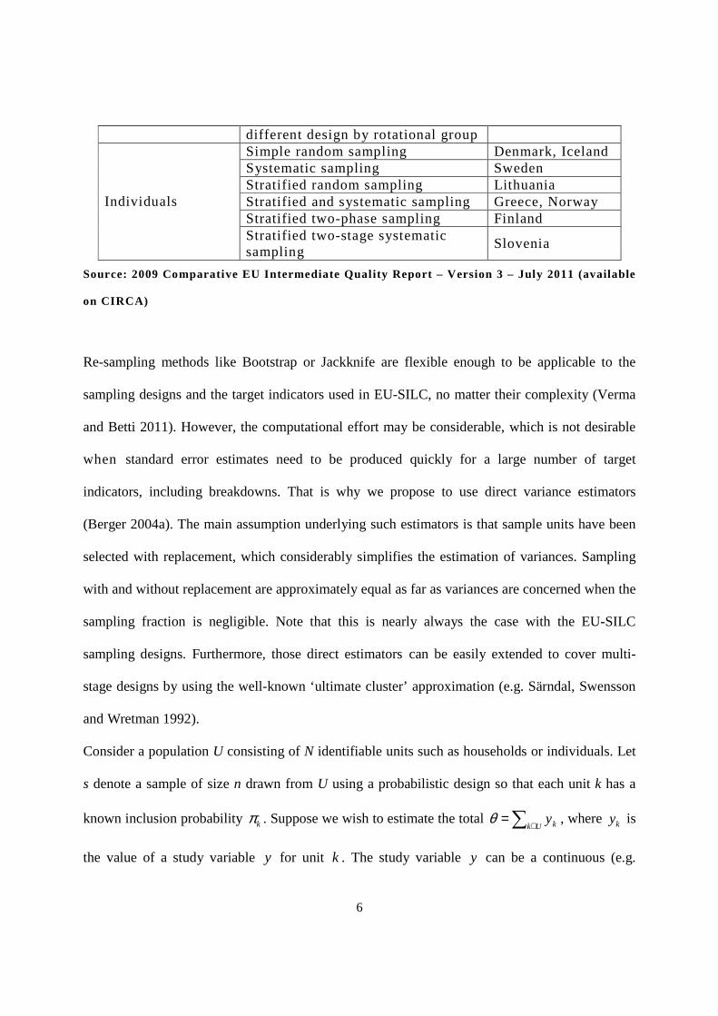
Table 1: EU-SILC sampling designs by country (2009)
Sampling unit
Sampling design Country
Dwellings/ addresses
Simple random sampling Malta Stratified simple random sampling Luxembourg Stratified random sampling from former participants of micro census
Germany
Stratified multi-stage sampling
Austria, Czech Republic, Spain, Poland, Portugal, Romania
Stratified multi-stage systematic sampling
France, Latvia, United Kingdom, Netherlands
Households
Stratified random sampling Cyprus, Slovakia, Switzerland
Stratified multi-stage sampling Ireland
Stratified multi-stage systematic sampling
Belgium, Bulgaria, Greece, Italy
Stratified sampling according to Hungary
6
different design by rotational group
Individuals
Simple random sampling Denmark, Iceland Systematic sampling Sweden Stratified random sampling Lithuania Stratified and systematic sampling Greece, Norway Stratified two-phase sampling Finland Stratified two-stage systematic sampling
Slovenia
Source: 2009 Comparative EU Intermediate Qual ity Report – Version 3 – July 2011 (available
on CIRCA)
Re-sampling methods like Bootstrap or Jackknife are flexible enough to be applicable to the
sampling designs and the target indicators used in EU-SILC, no matter their complexity (Verma
and Betti 2011). However, the computational effort may be considerable, which is not desirable
when standard error estimates need to be produced quickly for a large number of target
indicators, including breakdowns. That is why we propose to use direct variance estimators
(Berger 2004a). The main assumption underlying such estimators is that sample units have been
selected with replacement, which considerably simplifies the estimation of variances. Sampling
with and without replacement are approximately equal as far as variances are concerned when the
sampling fraction is negligible. Note that this is nearly always the case with the EU-SILC
sampling designs. Furthermore, those direct estimators can be easily extended to cover multi-
stage designs by using the well-known ‘ultimate cluster’ approximation (e.g. Särndal, Swensson
and Wretman 1992).
Consider a population U consisting of N identifiable units such as households or individuals. Let
s denote a sample of size n drawn from U using a probabilistic design so that each unit k has a
known inclusion probability kπ . Suppose we wish to estimate the total ∑ ∈=
Uk kyθ , where ky is
the value of a study variable y for unit k . The study variable y can be a continuous (e.g.
7
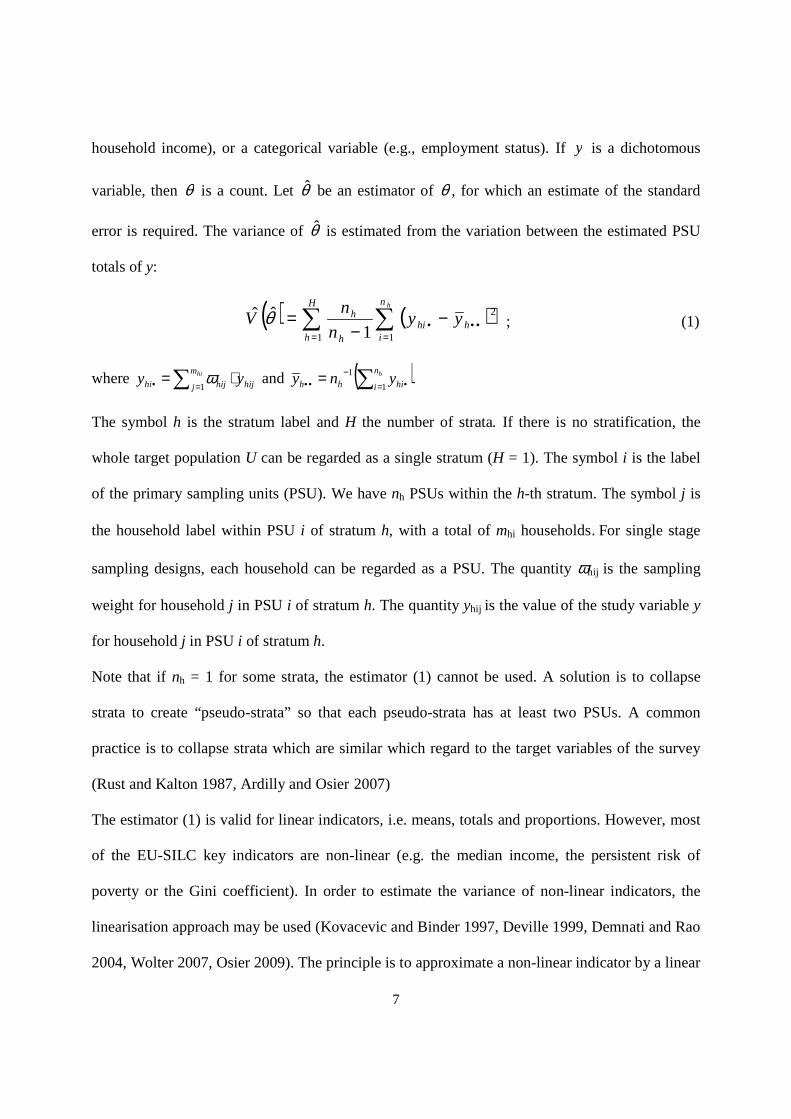
household income), or a categorical variable (e.g., employment status). If y is a dichotomous
variable, then θ is a count. Let θ̂ be an estimator of θ , for which an estimate of the standard
error is required. The variance of θ̂ is estimated from the variation between the estimated PSU
totals of y:
( ) ( )∑ ∑= =
••• −−
=H
h
n
ihhi
h
hh
yyn
nV
1 1
2
1ˆˆ θ ; (1)
where ∑ =• ⋅= him
j hijhijhi yy1ω and ( )∑ = •
−•• = hn
i hihh yny1
1
The symbol h is the stratum label and H the number of strata. If there is no stratification, the
whole target population U can be regarded as a single stratum (H = 1). The symbol i is the label
of the primary sampling units (PSU). We have nh PSUs within the h-th stratum. The symbol j is
the household label within PSU i of stratum h, with a total of mhi households. For single stage
sampling designs, each household can be regarded as a PSU. The quantity ωhij is the sampling
weight for household j in PSU i of stratum h. The quantity yhij is the value of the study variable y
for household j in PSU i of stratum h.
Note that if nh = 1 for some strata, the estimator (1) cannot be used. A solution is to collapse
strata to create “pseudo-strata” so that each pseudo-strata has at least two PSUs. A common
practice is to collapse strata which are similar which regard to the target variables of the survey
(Rust and Kalton 1987, Ardilly and Osier 2007)
The estimator (1) is valid for linear indicators, i.e. means, totals and proportions. However, most
of the EU-SILC key indicators are non-linear (e.g. the median income, the persistent risk of
poverty or the Gini coefficient). In order to estimate the variance of non-linear indicators, the
linearisation approach may be used (Kovacevic and Binder 1997, Deville 1999, Demnati and Rao
2004, Wolter 2007, Osier 2009). The principle is to approximate a non-linear indicator by a linear
8
form by retaining only the first-order term of a Taylor expansion. The variance of the linear
approximation can be used as an approximation of the variance of the non-linear indicator
considered. The linearisation procedure is justified on the basis of asymptotic properties of large
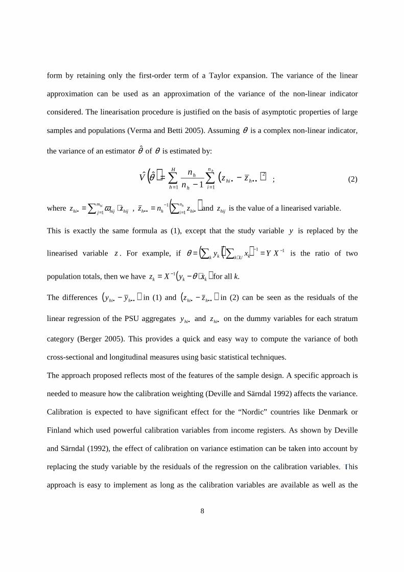
samples and populations (Verma and Betti 2005). Assuming θ is a complex non-linear indicator,
the variance of an estimator θ̂ of θ is estimated by:
( ) ( )∑ ∑= =
••• −−
=H
h
n
ihhi
h
hh
zzn
nV
1 1
2
1ˆˆ θ ; (2)
where ∑ =• ⋅= him
j hijhijhi zz1ω , ( )∑ = •
−•• = hn
i hihh znz1
1 and hijz is the value of a linearised variable.
This is exactly the same formula as (1), except that the study variable y is replaced by the
linearised variable z . For example, if ( )( ) 11 −−
∈== ∑∑ XYxy
Uk kk kθ is the ratio of two
population totals, then we have ( )kkk xyXz ⋅−= − θ1 for all k.
The differences ( )••• − hhi yy in (1) and ( )••• − hhi zz in (2) can be seen as the residuals of the
linear regression of the PSU aggregates •hiy and •hiz on the dummy variables for each stratum
category (Berger 2005). This provides a quick and easy way to compute the variance of both
cross-sectional and longitudinal measures using basic statistical techniques.
The approach proposed reflects most of the features of the sample design. A specific approach is
needed to measure how the calibration weighting (Deville and Särndal 1992) affects the variance.
Calibration is expected to have significant effect for the “Nordic” countries like Denmark or
Finland which used powerful calibration variables from income registers. As shown by Deville
and Särndal (1992), the effect of calibration on variance estimation can be taken into account by
replacing the study variable by the residuals of the regression on the calibration variables. This
approach is easy to implement as long as the calibration variables are available as well as the

9
initial weights before calibration or, equivalently, the calibration adjustment factors (also called
g-weights).
3. Extension to estimators of changes between two time points
The regression-based approach described in the previous section can be easily extended to cope
with estimators of changes between two time points (Berger and Priam 2013, Berger and Oguz
Alper 2013). Monitoring changes or trends in indicators over time is of key importance in many
areas of economic and social sciences.
In order to monitor trends towards agreed policy goals, we compare two cross-sectional estimates
for the same study variable taken on two different waves or occasions. The aim is to judge
whether the observed change is statistically significant. Therefore, interpreting differences
between point estimates may be misleading if temporal correlations between indicators is not be
taken into account properly. This would be relatively straightforward if estimates were based
upon independent samples. However, nearly all the EU-SILC countries have adopted a four-year
rotating structure (see Figure 1) as recommended by Eurostat, where individuals are interviewed
for a maximum of four years and 25% of the sample is refreshed every year with new individuals.

10
Figure 1: The EU-SILC four-year rotating structure
Berger and Priam (2013) proposed to use the residual variance matrix of a multivariate regression
model. The residual correlation matrix is used to produce estimates of correlation which are used
in the variance of the net change between indicators. The multivariate model includes covariates
which specify the stratification and interactions terms which specify the rotation of the sampling
designs. The estimator proposed by Berger and Priam (2013) is simpler to implement than the
estimators proposed by Munnich and Zins (2011), Nordberg (2000), Qualité (2009), Qualité and
Tillé (2008), Tam (1984) and Wood (2008). In particular cases, the proposed estimator reduces to
these estimators.
Sample at t
Sample at t+1
Sample at t+2
Sub-sample 1
Sub-sample 2
Sub-sample 3
Sub-sample 4
11
4. Preliminary results
We implemented the proposed regression-based approach to compute standard error estimates for
key EU-SILC cross-sectional measures, longitudinal measures and measures of changes. The first
indicator considered is the at-risk-of-poverty or social exclusion indicator (AROPE) and its three
sub-indicators: the at-risk-of-poverty rate (POV), the severe material deprivation rate (DEP) and
the share of individuals aged less than 60 living in households with very low work intensity
(LWI) (Eurostat 2012b). The at-risk-of-poverty or social exclusion (AROPE) is the “Europe
2020” headline indicator on poverty and social exclusion. It counts the number of individuals
living in households which are at-risk-of-poverty, severely materially deprived or with very low
work intensity; the individuals present in several sub-indicators being counted only once
(Eurostat 2013). The change in the AROPE between two years is also considered. We also
consider the persistent at-risk-of-poverty rate, which is the key EU-SILC longitudinal indicator.
The persistent risk of poverty is defined as having an equivalised disposable income below the at-
risk-of-poverty threshold in the current year and in at least two of the preceding three years.
The estimates are based upon anonymised EU-SILC micro-data files that are provided by
Eurostat for statistical/research purposes only. Since research files do not include any stratum
identification number nor calibration variables, we had to use NUTS2 region as a proxy for
stratification and ignore the impact of calibration on the variance estimates.
4.1. Cross-sectional measures
In table 2, we have the estimator of the standard error for the at-risk-of-poverty rate (POV), the
severe material deprivation rate (DEP), the share of individuals aged less than 60 living in
households with very low work intensity (LWI) and the AROPE.

12
The standard error estimates for the AROPE lies between 0.5 and 1 percentage point in most of
the countries, which means that the absolute margin of error for the indicators (based on
normality assumption) lies between ±1 and ±2 percentage points. The standard errors are greater
than 1 point in Bulgaria, Lithuania and Romania; while they are lower than 0.5 point in Germany
and Sweden.
As far as the AROPE’s three sub-indicators are concerned (POV, DEP, LWI), the standard error
estimates appear lower than those calculated for the AROPE because, by definition, the AROPE
indicator reaches higher values than its three components. For example, the estimated standard
errors for the severe material deprivation rates are relatively low for some countries (e.g. 0.1
percentage point for Sweden and 0.2 point for Luxembourg).
Table 2: Standard error estimates for the at-risk-of-poverty or social exclusion indicator
(AROPE) and its three sub-indicators, 2011
At-risk-of-poverty rate (POV)
Severe material deprivation rate (DEP)
Share of individuals living aged < 60 living in
households with very low work intensity (LWI)
At-risk-of-poverty or social exclusion
(AROPE)
Indicator value (%)
Estimated standard error (% points)
Indicator value (%)
Estimated standard error (% points)
Indicator value (%)
Estimated standard error (% points)
Indicator value (%)
Estimated standard error (% points)
Austria 12,6 0,58 3,9 0,35 8,0 0,51 16,9 0,63
Belgium 15,3 0,86 5,7 0,53 13,7 0,87 21,0 0,98
Bulgaria 22,2 0,97 43,5 1,07 11,0 0,75 49,0 1,07
Switzerland 15,0 0,57 1,0 0,26 4,7 0,41 17,2 0,61
Cyprus 14,5 0,66 10,7 0,70 4,5 0,36 23,5 0,85
Czech Republic 9,8 0,49 6,1 0,41 6,6 0,43 15,3 0,57
Germany 15,8 0,38 5,3 0,23 11,1 0,38 19,9 0,41
Denmark 13,0 0,71 2,6 0,35 11,4 0,76 18,9 0,77
Estonia 17,5 0,65 8,7 0,48 9,9 0,57 23,1 0,73
Greece 21,4 0,78 15,2 0,77 11,8 0,69 31,0 0,94
Spain 21,8 0,55 3,9 0,27 12,2 0,45 27,0 0,58
Finland 13,7 0,45 3,2 0,24 9,8 0,45 17,9 0,50
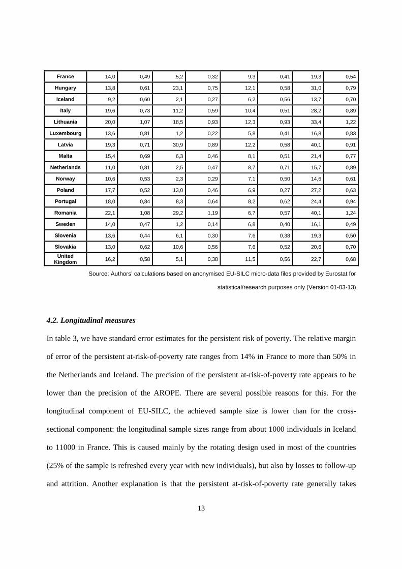
13
France 14,0 0,49 5,2 0,32 9,3 0,41 19,3 0,54
Hungary 13,8 0,61 23,1 0,75 12,1 0,58 31,0 0,79
Iceland 9,2 0,60 2,1 0,27 6,2 0,56 13,7 0,70
Italy 19,6 0,73 11,2 0,59 10,4 0,51 28,2 0,89
Lithuania 20,0 1,07 18,5 0,93 12,3 0,93 33,4 1,22
Luxembourg 13,6 0,81 1,2 0,22 5,8 0,41 16,8 0,83
Latvia 19,3 0,71 30,9 0,89 12,2 0,58 40,1 0,91
Malta 15,4 0,69 6,3 0,46 8,1 0,51 21,4 0,77
Netherlands 11,0 0,81 2,5 0,47 8,7 0,71 15,7 0,89
Norway 10,6 0,53 2,3 0,29 7,1 0,50 14,6 0,61
Poland 17,7 0,52 13,0 0,46 6,9 0,27 27,2 0,63
Portugal 18,0 0,84 8,3 0,64 8,2 0,62 24,4 0,94
Romania 22,1 1,08 29,2 1,19 6,7 0,57 40,1 1,24
Sweden 14,0 0,47 1,2 0,14 6,8 0,40 16,1 0,49
Slovenia 13,6 0,44 6,1 0,30 7,6 0,38 19,3 0,50
Slovakia 13,0 0,62 10,6 0,56 7,6 0,52 20,6 0,70
United Kingdom 16,2 0,58 5,1 0,38 11,5 0,56 22,7 0,68
Source: Authors’ calculations based on anonymised EU-SILC micro-data files provided by Eurostat for
statistical/research purposes only (Version 01-03-13)
4.2. Longitudinal measures
In table 3, we have standard error estimates for the persistent risk of poverty. The relative margin
of error of the persistent at-risk-of-poverty rate ranges from 14% in France to more than 50% in
the Netherlands and Iceland. The precision of the persistent at-risk-of-poverty rate appears to be
lower than the precision of the AROPE. There are several possible reasons for this. For the
longitudinal component of EU-SILC, the achieved sample size is lower than for the cross-
sectional component: the longitudinal sample sizes range from about 1000 individuals in Iceland
to 11000 in France. This is caused mainly by the rotating design used in most of the countries
(25% of the sample is refreshed every year with new individuals), but also by losses to follow-up
and attrition. Another explanation is that the persistent at-risk-of-poverty rate generally takes

14
lower value than the cross-sectional at-risk-of poverty rate (POV) or the AROPE indicator.
Finally, the higher dispersion of the longitudinal sampling weights, which are adjusted at each
wave for attrition and calibration to external data sources, is likely to reduce the precision of the
persistent risk of poverty.
Table 3 – Standard error estimates and confidence intervals for the persistent at-risk-of-
poverty rate, 2006-2009
Persistent at-risk-of-poverty rate (%)
Confidence interval (Empirical Likelihood - EL)
Confidence interval (Central Limit Theorem - CLT)
Lower Upper Lower Upper
Austria 5.93 4.59 7.73 4.38 7.47
Belgium 8.94 7.10 11.31 6.89 10.98
Bulgaria 10.67 8.20 13.87 7.92 13.42
Cyprus 10.95 9.13 13.10 8.88 13.02
Czech Republic
3.55 2.53 5.13 2.33 4.77
Denmark 6.27 4.58 8.43 4.39 8.15
Estonia 12.97 11.13 15.13 10.91 15.04
Spain 11.1 9.49 12.95 9.40 12.80
Finland 6.91 5.55 8.59 5.37 8.45
France 6.92 6.04 7.92 6.00 7.84
Greece 14.5 11.76 17.84 11.76 17.25
Hungary 8.28 6.60 10.41 6.46 10.10
Ireland 6.34 4.34 9.54 3.74 8.94
Iceland 4.17 2.36 6.89 1.97 6.38
Italy 13.38 11.16 16.04 11.28 15.48
Lithuania 11.73 9.18 15.19 8.91 14.54
Luxembourg
8.82 6.88 11.47 6.66 10.98
Latvia 17.74 13.96 23.94 13.48 22.01
Malta 6.21 4.62 8.21 4.40 8.03
Netherlands 6.36 4.10 9.78 3.73 9.00
Norway 5.36 4.15 6.93 4.03 6.70
Poland 10.16 7.54 13.43 8.62 11.71
Portugal 9.98 7.81 12.67 7.60 12.36
Sweden 5.66 4.38 7.24 4.24 7.07
Slovakia 5.01 3.54 7.11 3.30 6.72
United Kingdom
8.36 6.66 10.48 6.51 10.21

15
Source: Authors’ calculations based on anonymised EU-SILC micro-data files provided by Eurostat for
statistical/research purposes only (Version 01-03-13)
In table 3, we also have the empirical likelihood (EL) confidence intervals based on a novel
approach proposed by Berger and De la Riva Torres (2012). These intervals have better coverage
than the intervals based upon the Central limit theorem (CLT). The difference between the CLT
confidence intervals and the EL confidence intervals are due to the lack of normality of the
sampling distribution.
4.3. Standard errors of measures of changes
In table 4, we have the standard error estimates and confidence intervals (based on normality
assumption) for changes in the AROPE between 2010 and 2011. The computations were made
within Eurostat premises using the EU-SILC Production Data Base (EU-SILC PDB). In this case,
we use the right stratification variable. If a confidence interval does not include 0, we can say the
difference between 2010 and 2011 is statistically significant (at a given level of confidence).
Table 4 – Estimated standard errors for estimators of net change in the AROPE between
2010 and 2011
AROPE
(%) - 2010 AROPE
(%) - 2011
(2011) - (2010)
(% points)
Estimated standard error (% points)
Confidence interval at
95% - Lower bound
Confidence interval at
95% - Upper bound
Is the difference significant (Y/N)?
Austria 16,6 16,9 0,34 0,47 -0,58 1,26 N
Belgium 20,8 21,0 0,14 0,70 -1,23 1,51 N
Bulgaria 49,2 49,1 -0,04 0,76 -1,53 1,44 N
Switzerland 17,2 17,2 0,02 0,37 -0,71 0,74 N
Cyprus 23,5 23,7 0,24 0,65 -1,05 1,52 N
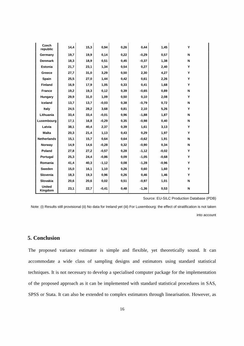
16
Czech republic 14,4 15,3 0,94 0,26 0,44 1,45 Y
Germany 19,7 19,9 0,14 0,22 -0,29 0,57 N
Denmark 18,3 18,9 0,51 0,45 -0,37 1,38 N
Estonia 21,7 23,1 1,34 0,54 0,27 2,40 Y
Greece 27,7 31,0 3,29 0,50 2,30 4,27 Y
Spain 25,5 27,0 1,44 0,42 0,61 2,26 Y
Finland 16,9 17,9 1,05 0,33 0,41 1,68 Y
France 19,2 19,3 0,12 0,39 -0,65 0,89 N
Hungary 29,9 31,0 1,09 0,50 0,10 2,08 Y
Iceland 13,7 13,7 -0,03 0,38 -0,79 0,72 N
Italy 24,5 28,2 3,68 0,81 2,10 5,26 Y
Lithuania 33,4 33,4 -0,01 0,96 -1,88 1,87 N
Luxembourg 17,1 16,8 -0,29 0,35 -0,98 0,40 N
Latvia 38,1 40,4 2,37 0,39 1,61 3,13 Y
Malta 20,3 21,4 1,13 0,43 0,29 1,97 Y
Netherlands 15,1 15,7 0,64 0,64 -0,62 1,91 N
Norway 14,9 14,6 -0,28 0,32 -0,90 0,34 N
Poland 27,8 27,2 -0,57 0,28 -1,12 -0,02 Y
Portugal 25,3 24,4 -0,86 0,09 -1,05 -0,68 Y
Romania 41,4 40,3 -1,12 0,08 -1,28 -0,96 Y
Sweden 15,0 16,1 1,10 0,26 0,60 1,60 Y
Slovenia 18,3 19,3 0,96 0,26 0,46 1,46 Y
Slovakia 20,6 20,6 0,02 0,51 -0,97 1,01 N
United Kingdom 23,1 22,7 -0,41 0,48 -1,36 0,53 N
Source: EU-SILC Production Database (PDB)
Note: (i) Results still provisional (ii) No data for Ireland yet (iii) For Luxembourg: the effect of stratification is not taken
into account
5. Conclusion
The proposed variance estimator is simple and flexible, yet theoretically sound. It can
accommodate a wide class of sampling designs and estimators using standard statistical
techniques. It is not necessary to develop a specialised computer package for the implementation
of the proposed approach as it can be implemented with standard statistical procedures in SAS,
SPSS or Stata. It can also be extended to complex estimators through linearisation. However, as

17
the linearisation procedure is justified on the basis of asymptotic properties, variance estimates
may not be reliable if the sample size is not sufficiently large.
The numerical results obtained using this approach seem plausible, although they have to be
interpreted with caution given the lack of sampling design information in the EU-SILC user data
files and potential quality problems with the current design variables. Eurostat is currently
working with Net-SILC2 to improve the situation. Concrete recommendations have already been
made for better recording of sampling design variables in EU-SILC (Goedemé 2013b).
A major shortcoming of the proposed approach is that it does not take the imputation variance
into account. However, the income variables have been heavily imputed, with different
imputation methods used across countries. For simplicity, imputed values have been treated as
true values. However, this assumption may lead to severely under-estimating the variance,
particularly when the proportion of imputed values is important (Rao and Shao 1992). Variance
estimation under imputation is not an easy task. Direct variance formulas are usually very
complex (Deville and Särndal 1994) and method-specific. For example, for hot-deck imputation,
Berger and Escobar (2012) proposed an approach to estimate the variance of change in the
presence of imputed values. Thus, it does not seem realistic to try to estimate the imputation
variance on a streamline basis, especially when the imputation methods vary greatly from one
country to another. Nevertheless, the imputation variance may be estimated occasionally using
for instance the SAS software SEVANI developed by Statistics Canada (Beaumont and
Bissonnette 2011). It would be useful to develop a “rule of the thumb” approach which would
take into account of the effect of imputation.
The proposed approach can be implemented with any rotating longitudinal survey as long as the
sampling fraction is negligible. Berger (2004b) proposed a variance estimator for change which is
more complex and can be used with large sampling fractions. With small sampling fraction,
18
Berger and Priam (2013) showed that the estimator proposed in this paper is asymptotically equal
to Berger (2004b) estimator. In a series of simulation based on the Swedish Labour Force Survey,
Andersson et al. (2011) showed that for estimation of strata domains the variance estimator
proposed by Berger (2004a) gives accurate variance estimates.
Empirical likelihood confidence intervals (Berger and De la Riva Torres 2012) are an alternative
way to measure the accuracy of indicators. This approach does not require analytic derivation of
variances, linearisation or resampling. Its implementation is relatively simple, but requires a
specialised computer package (currently developed in R at the University of Southampton).
Acknowledgement: We wish to thank Omar de la Riva Torres (University of Southampton) for
calculating the empirical likelihood confidence intervals for table 3.
References
• Andersson, C., Andersson, K. and Lundquist, P. (2011) Variansskattningar avseende
forandringsskattningar i panelundersokningar (variance estimation of change in panel
surveys). Methodology reports from Statistics Sweden (Statistiska centralbyran).
• Ardilly, P. and Osier, G. (2007). Cross-sectional variance estimation for the French
“Labour Force Survey”. Survey Research Methods, 1, 2, pp. 75-83. Available at: URL =
http://w4.ub.uni-konstanz.de/srm/article/viewPDFInterstitial/77/55
• Atkinson, A. B. and Marlier, E. (2010) Income and living conditions in Europe.
Luxembourg: Office for Official Publications. Available at: URL =
http://epp.eurostat.ec.europa.eu/cache/ITY_OFFPUB/KS-31-10-555/EN/KS-31-10-555-
EN.PDF

19
• Beaumont, J.-F. and Bissonnette, J. (2011). Variance Estimation under Composite
Imputation: The Methodology Behind SEVANI. Survey Methodology, vol. 37, pp. 171-
179.
• Berger, Y. G. (2004a). A Simple Variance Estimator for Unequal Probability Sampling
Without Replacement. Journal of Applied Statistics, 3, 305-315.
• Berger, Y. G. (2004b) Variance estimation for measures of change in probability
sampling. Canadian Journal of Statistics, 32, 451–467.
• Berger, Y. G. (2005) Variance estimation with highly stratified sampling designs with
unequal probabilities. Australian and New Zealand Journal of Statistics, 47, 365–373.
• Berger, Y. G. and De La Riva Torres, O. (2012) A unified theory of empirical like- lihood
ratio confidence intervals for survey data with unequal probabilities and non negligible
sampling fractions,Working paper. http://eprints.soton.ac.uk/337688/
• Berger, Y. G. and Escobar, E. L. (2012). Variance estimation of imputed estimators of
change over time from repeated surveys. In Journées de Méthodologie Statistiques 2012,
Paris, FR, 24-26 Jan 2012. 8pp.
• Berger, Y. G. and Oguz Alper, M. (2013). Variance estimation of change of poverty based
upon the Turkish EU-SILC survey. Paper presented at the NTTS (New Techniques and
Technologies for Statistics) Conference, Brussels, 5-7 March 2013.
• Berger, Y. G. and Priam, R. (2013). A simple variance estimator of change for rotating
repeated surveys: an application to the EU-SILC household surveys. University of
Southampton, Statistical Sciences Research Institute. Available at: URL =
http://eprints.soton.ac.uk/347142
20
• Demnati, A. and Rao, J. N. K. (2004). Linearization variance estimators for survey data.
Survey Methodology, 30, 17-26.
• Deville, J-C. (1999). Variance estimation for complex statistics and estimators:
linearization and residual techniques. Survey Methodology, December 1999, 25, 2, 193-
203.
• Deville, J-C. and Särndal, C-E. (1992). Calibration estimators in survey sampling. Journal
of the American Statistical Association, 87, 418, 376-382.
• Deville, J-C. and Särndal, C-E. (1994). Variance Estimation for the Regression Imputed
Horvitz-Thompson Estimator. Journal of Official Statistics, 10, 4, 381–394.
• Eurostat (2012a) European Union statistics on income and living conditions (EU-SILC).
http://epp.eurostat.ec.europa.eu/portal/page/portal/microdata/eu_silc. [Online; accessed 7
Jan. 2013].
• Eurostat (2012b) People at risk of poverty or social exclusion (EU-SILC).
http://epp.eurostat.ec.europa.eu/portal/page/portal/product_details/dataset?p_product_cod
e=T2020_50. [Online; accessed 7 Jan. 2013]].
• Goedemé, T. (2010). The construction and use of sample design variables in EU-SILC. A
user’s perspective. Report prepared for Eurostat. Available at: URL =
http://www.centrumvoorsociaalbeleid.be/index.php?q=node/2157/en
• Goedemé, T. (2013a). How much Confidence can we have in EU-SILC? Complex
Sample Designs and the Standard Error of the Europe 2020 Poverty Indicators. Social
Indicators Research, vol. 110, no. 1, pp. 89-110
• Goedemé, T. (2013b). The EU-SILC sample design variables: critical review and
recommendations. CSB Working paper 13/02, Antwerp: Herman Deleeck Centre for
21
Social Policy – University of Antwerp. Available at:
http://www.centrumvoorsociaalbeleid.be/index.php?q=node/3891
• Kalton G. (2009). Design for surveys over time. Handbook of Statistics: Design, Method
and Applications: D. Pfeffermann and C.R. Rao. (editors). Elsevier.
• Kovacevic, M. and Binder, D.A. (1997). Variance Estimation for Measures of Income
Inequality and Polarization – The Estimating Equations Approach. Journal of Official
Statistics, 13, 1, 41-58.
• Muennich, R. and Zins, S. (2011). Variance estimation for indicators of poverty and social
exclusion. Work-package of the European project on Advanced Methodology for
European Laeken Indicators (AMELI).
Available at URL = http://www.uni-trier.de/index.php?id=24676. [Online; accessed 4 Jan.
2013].
• Nordberg, L. (2000). On variance estimation for measures of change when samples are
coordinated by the use of permanent random numbers. Journal of Official Statistics, 16,
363–378.
• Osier, G. (2009). Variance estimation for complex indicators of poverty and inequality
using linearization techniques. Survey Research Methods, 3, 3, 167-195. Available at:
URL = http://w4.ub.uni-konstanz.de/srm/article/view/369
• Qualité, L. (2009). Unequal probability sampling and repeated surveys. PhD Thesis,
University of Neuchatel, Switzerland.
• Qualité, L. and Tillé, Y. (2008). Variance estimation of changes in repeated surveys and
its application to the Swiss survey of value added. Survey Methodology, 34, 173–181.

22
• Rao, J. N. K. and Shao, A. J. (1992). Jackknife variance estimation with survey data under
hotdeck imputation. Biometrika, 79, 811-822.
• Rust, K. and Kalton, G. (1987). Strategies for collapsing strata for variance estimation.
Journal of Official Statistics, 3, 1, 69-81.
• Särndal, C-E., Swensson, B. and Wretman, J. (1992). Model Assisted Survey Sampling.
Springer Series in Statistics.
• Tam, S. M. (1984). On covariances from overlapping samples. American Statistician, 38,
288–289.
• Verma, V. and Betti, G. (2005). Sampling errors and design effects for poverty measures
and other complex statistics. University of Siena, working paper n°53. Available at: URL
= http://www.econ-pol.unisi.it/dmq/pdf/DMQ_WP_53.pdf
• Verma, V. and Betti, G. (2011). Taylor linearization sampling errors and design effects
for poverty measures and other complex statistics. Journal of Applied Statistics, 38, 8,
1549-1576.
• Wolter, K. M. (2007). Introduction to Variance Estimation. 2nd ed. New York: Springer.
• Wood, J. (2008). On the covariance between related Horvitz-Thompson estimators.
Journal of Official Statistics, 24, 53–78.