STABILIZATION AND ADJUSTMENT POLICIES AND PROGRAMMES

RESEARCH ADVISERS: Professors Lance Taylor and G K Helleiner

COUNTRY STUDY: ARGENTINA

Authors: Jose Maria Fanelli CEDES (Centro de Estudios de Estado y Sociedad) Argentina Roberto Frenkel CEDES Argentina Carlos Winograd CEDES Argentina

WORLD INSTITUTE FOR DEVELOPMENT ECONOMICS RESEARCH Lal Jayawardena, Director

The Board of WIDER:

Saburo Okita, Chairman Reimut Jochimsen Abdlatif Y. Al-Hamad Pentti Kouri Bernard Chidzero Carmen Miro Mahbub ul Haq I. G. Patel Albert 0. Hirschman Soedjatmoko (ex officio) Lai Jayawardena (ex officio) Janez Stanovnik

(WIDER) was established in 1984 and started work in Helsinki in the spring of 1985. The principal purpose of the Institute is to help identify and meet the need for policy-oriented socio-economic research on pressing global and development problems and their inter-relationships. The establishment and location of WIDER in Helsinki have been made possible by a generous financial contribution from the Government of Finland.

The work of WIDER is carried out by staff researchers and visiting scholars and through networks of collaborating institutions and scholars in various parts of the world.

WIDER*s research projects are grouped into three main themes:

I. Hunger and poverty - the poorest billion II. Money, finance and trade - reform for world development III. Development and technological transformation - the

management of change

WIDER seeks to involve policy makers from developing countries in its research efforts and to draw specific policy lessons from the research results. The Institute continues to build up its research capacity in Helsinki and to develop closer contacts with other research institutions around the world.

In addition to its scholarly publications, WIDER issues short, non-technical reports aimed at policy makers and their advisers in both developed and developing countries. WIDER will also publish a series of study group reports on the basic problems of the global economy.

TABLE OF CONTENTS

Page

PREFACE BY THE DIRECTOR

EXECUTIVE SUMMARY

INTRODUCTION

SHORT-RUN ECONOMIC POLICY 1

1. The failure of traditional orthodoxy (1976-79) 1 2. The failure of the new orthodoxy:

active crawling peg (1979-81) 3 3. The chaotic adjustment (1981-83) 5

A LONG-RUN VIEW 10

1. Inflation and relative prices 10 2. Real sector and growth 11 3. Balance of payments and foreign debt 13 4. Investment, savings and debt 15

STRUCTURAL FEATURES OF THE ARGENTINE ECONOMY 20

1. Real sector 20 2. Financial sector 25 3. Dynamic of inflation 34

THE AUSTRAL PLAN: AN ATTEMPT TO DO IT BETTER 40

1. Learning from the past 40 2. The Austral plan 41

(a) Monetary reform 42 (b) Fiscal adjustment and external debt 43 (c) Prices, wages and the exchange rate 44

3. Behaviour of the economy 45 (a) The freezing (June 1985 - March 1986) 46 (b) Lifting the freeze (April - September 1986) 48 (c) Administered prices and active monetary

policy (September 1986) 50 4. The future 51

APPENDIX 54

FOOTNOTES 57

REFERENCES 61

TABLES 64

FIGURES 72

PREFACE BY THE DIRECTOR

This monograph is part of a series being published by WIDER on the experience of developing countries with stabilization and adjustment programmes in the 1970s and 1980s. Each study analyzes the package of policies implemented by a specific country; its relations with the IMF and World Bank; the effects of the policies on production, employment, the balance of payments and social welfare; and what other policies might have been followed instead.

The intention of the series is to assist developing countries to devise adjustment policies that would, while accomplishing desirable adjustment and growth objectives, simultaneously remain politically viable in the particular country settings studied.

For this purpose it was thought desirable to explore policy alternatives to the adjustment programmes being implemented. Built into the design of the series, therefore - and constituting indeed its special feature - is the requirement that each study include a 'counterfactual' exercise to illustrate the effects of alternative policies. Utilizing econometric models adapted or specifically developed for each country, the probable effects of alternative policy packages are estimated; the object was to see how far the balance-of-payments adjustment and growth goals of a particular programme might have been achieved at a possibly lower social cost with a different policy mix.

Each country study is written by an independent scholar and expert in the relevant country. First drafts of the studies in this series were discussed at the WIDER conference on stabilization and adjustment policies in developing countries which was held 19-22 August, 1986 in Helsinki. Each study has been reviewed by WIDER's research advisers for the project, Professors Gerry Helleiner and Lance Taylor, and revised substantively by the author as necessary; subsequent editing has been conducted under the overall supervision of Mr Robert Pringle, Senior Fellow, who serves also as editorial adviser on WIDER publications.

A companion volume by Professor Taylor summarizing the experience of the countries surveyed will draw broader implications for the theory and practice of stabilization and adjustment policies; this volume will be published by Oxford University Press. The individual country studies in this series will subsequently be grouped into separate volumes, also for eventual publication by Oxford University Press.

Lal Jayawardena Director March 1987

EXECUTIVE SUMMARY

Argentina has had successive stabs at stabilization since the mid-1970s. Throughout most of this time it has had to wrestle with acute problems of hyperinflation, capital flight, rising external debt, a stop-go pattern of output, and for a long time a heavily depressed level of real wages. It has tried orthodox stabilization policies, a more monetarist approach, and what can perhaps be described as 1 ad hocery'.

In June 1985 these efforts culminated in the Austral plan, a type of shock treatment to change inflation expectations. Essentially, this consisted of a price freeze, tight control of the monetary and fiscal aggregates, and a currency reform.

Initially, the results were encouraging. Inflation fell, output recovered and the trade balance was in surplus. But short-run success will be converted into long-run stability, the authors argue, only if international economic conditions prove helpful and, in particular, if the burden of servicing Argentina's heavy external debt is eased by an adequate flow of fresh credits.

I. INTRODUCTION

The purpose of this paper is to investigate the effects

on the structure and functioning of the Argentine economy of

the programmes and policies implemented in the last ten

years in an effort to achieve short-run stabilization.

The work is organized in four sections. The first

describes the main economic policies implemented in

Argentina over the past decade; it is aimed at readers

unfamiliar with the country's recent economic experience.

The second section provides a long-run view of the evolution

of the Argentine economy.

The third interprets the workings and structural

features of the Argentine economy in terms of stylized

facts. In the last section, the Austral plan is analyzed.

Appended to the paper is the algebra used in the third

section.

We are indebted to Gerald Helleiner, Nora Lustig and Lance

Taylor for helpful comments on an early draft of this paper.

1.

II. SHORT-RUN ECONOMIC POLICY

1. The failure of traditional orthodoxy (1976-79)

As explained more fully later, 1975 was a crucial

turning point for the Argentine economy. By the beginning of

1976 the economy was characterized by a runaway fiscal

deficit, external bottlenecks caused by both a current

account deficit and capital flight, and a rate of increase

in domestic prices approaching hyperinflation. In response,

the military government in 1976-77 signed two successive

agreements with the IMF. Structural reforms were also

initiated by liberalization in two areas: the financial

system and external trade.

Stabilization policy centered on effecting a radical

change in relative prices. Between March and May 1976 the

nominal exchange rate for imports rose by 162 per cent,

state controlled prices by 137 per cent, industrial prices

by 144 per cent and consumer prices by 106 per cent. The

increase in nominal wages was a mere 20 per cent. Real wages

thus fell markedly and remained depressed until 1979. The

increase in the real exchange rate and the reduction in real

wages led to a redistribution of income from wage earners to

profits. This in turn led to a reduction in aggregate demand

which led to lower imports, reducing pressure on the balance

of payments.

In 1977 the program had been in effect for a year and

government officials were highly optimistic. The balance of

payments outlook was excellent: the trade surplus had

reached US$ 880 million in 1976 and the current account

suprlus US$ 650 million. In the meantime, higher investment

and exports led in the last months of 1976 to an increase in

overall economic activity.

Inflation, however, had not been brought under control.

In the last four months of 1976 price rises accelerated,

reaching an average of 10 per cent a month as against 4.1

2.

per cent in the third quarter. Inflation became the central

preoccupation of stabilization policy. Following a brief

experiment with price controls, the last quarter of 1977 saw

monetary policy become the main tool of anti-inflationary

strategy. This was also the quarter of the reform of the

financial sector, which in McKinnon's terms was

'de-repressed': interest rates were set free to fluctuate

according to market forces, and quantitative constraints on

credit were eliminated. This had far-reaching effects.

Prior to financial reform, the government had not used

monetary policy as an active instrument of economic

adjustment. But once persistent inflation had been diagnosed

to be the consequence of excessive money creation, the rate

of growth of the monetary aggregates was reduced, leading to

a sudden sharp drop in the real money supply. Given the

rising nominal demand for credit, the decline in the supply

of real money provoked a sharp increase in nominal interest

rates from a monthly average of 0.4 per cent in the third

quarter of 1977 to 4.6 per cent in the fourth quarter.

Higher interest rates in turn led rapidly to the contraction

of aggregate demand and production. Total investment dropped

by 8.5 per cent in the fourth quarter of 1977, and the

recession extended into the first quarter of 1978.

Although the increase in nominal interest rates had no

disinflationary impact, it was effective in securing foreign

capital attracted by the possibility of earning higher

returns in Argentina than elsewhere. The contraction in

domestic credit was thus partially offset in 1978 by an

inflow of foreign capital, which jeopardized control of the

money supply. Indeed, traditional monetarism in the context

of financial liberalization showed little success in the

short run: the main features of the Argentine economy

following a year of stabilization were recession, higher

inflation and speculative capital inflows. The failure of

traditional monetarism opened the way for a new

anti-inflationary policy which was put into practice at the

beginning of 1979.

3.

2. The failure of the new orthodoxy: active crawling

peg (1979-81)

In December 1978 a new stabilization plan was announced.

It centred on predetermining the trend in the exchange rate

over a given period of time. The exchange rule established

that the peso would be devalued monthly at a rate

diminishing progressively from 5.25 per cent in February

1979 to zero in March 1981. The plan assumed that, from that

point on, domestic inflation would be identical with the

external rate.

The exchange rule was complemented by rules for public

prices and domestic money supply consistent with the

devaluation target. Wages were exposed to a much higher

degree of market determination as collective agreements by

economic sectors were replaced by decentralized negotiations

at the firm level. Various import restrictions were lifted

and virtually no controls were placed on the foreign

exchange market. The stabilization plan assumed that by

fixing in advance the exchange rate and public prices,

inflationary expectations would diminish. If this mechanism

failed, import competition would discipline

'inflation-biased1 firms. It was expected that

liberalization and the integration of the domestic capital

and goods markets into the world market would allow short

and long-run targets to converge.

The theoretical framework for all these policy measures

was provided by a monetary approach to the balance of

payments. Under the assumptions used in this approach, the

pre-announced rate of devaluation appeared to be an

efficient stabilization strategy. Disinflation could be

achieved with no cost in terms of employment or production.

The law of one price and capital mobility would guarantee

that domestic inflation and the nominal interest rate would

both decrease in accordance with a declining rate of

devaluation which was known with certainty by economic

agents. The domestic real interest rate would come to equal

4.

the international rate, and balance-of-payments performance

would be determined by domestic monetary policy.

The effects of the experiment were not up to the

expectations of its authors. First, the law of one price did

not hold in this instance: the crawling peg devaluation rule

was very powerful in influencing the prices of tradable

goods, but not of wages and non-tradable goods.

Consequently, the domestic rate of inflation was

systematically higher than the one predicted by the exchange

rate rule and by external inflation. In 1979 the peso was

devalued by 63 per cent while the inflation rate was 159.5

per cent (CPI). In 1980 devaluation was 24.3 per cent while

prices rose by 100.8 per cent. Secondly, the nominal

domestic interest rate was higher than predicted because the

risk premium - defined as the difference between nominal

domestic interest rates and the cost of external credit -

showed an increasing trend. In effect, as the lagging

exchange rate led to an increasing current account deficit

and to a widespread belief that the exchange rate rule would

be broken, the expectation of an 'unexpected' devaluation

raised exchange risk and nominal interest rates.

The lack of convergence between the actual and expected

values of the exchange rate induced cumulative and explosive

disequilibria which were to change profoundly the country's

economic structure. The overvaluation of the peso at a time

when the economy was being opened up to foreign capital and

goods markets provoked a sharp decrease in net exports of

goods and services, mainly as a consequence of rising

imports. Imports as a percentage of GDP, which averaged 7.3

per cent in 1970-78, reached the hitherto unheard-of level

of 15 per cent in 1980-81. In addition, monetary policy in

1979 at the beginning of the plan widened the spread between

the internal and external cost of credit, resulting in

massive capital inflows and a significant increase in

reserves. A short-lived illusion of external solvency arose.

As the exchange rate rule began to lose its credibility, the

flow of speculative capital was reversed and previously

5.

accumulated foreign exchange headed for more secure shores.

One result of this reversal was that net external indebtness

jumped from $ 6,500 million in December 1978 to $ 19,500

million at the end of 1980 (see table 5).

In order that the subsequent evolution of the economy is

understood, it needs to be stressed that the aggregate

figures for capital flows hide very different patterns of

behaviour on the part of public and private sector actors

respectively. Both sectors shoved net capital inflows in

1979. In 1980, however, Argentinians lost confidence in the

active crawling peg policy and began to buy up foreign

exchange. The public sector compensated for this by stepping

up its external borrowing, which in 1980 increased by 45 per

cent. The increase in the public external debt during the

first quarter of 1981 was almost equal to that of the entire

previous year. It was insufficient, however, to compensate

for the flight of private capital, and the active crawling

peg policy had to be abandoned. In February 1981 the

government was forced to decree an unheralded 10 per cent

devaluation in an effort to halt the depletion of Central

Bank reserves. This measure was utterly useless in

correcting the disequilibria and the experiment with the

'new orthodoxy' came to an end. Its consequences, however,

were just beginning to be felt.

3. The chaotic adjustment (1981-83)

The three years after the crisis generated by the active

crawling peg policy were chaotic in that the external and

internal disequilibria produced by the active crawling peg

experience were not tackled with a set of consistent

economic policies. At the beginning of 1981 the economy

showed a large current account deficit, a sharp decline in

overall activity, and a financial crisis. From that point on

inflation accelerated rapidly.

In a context of high political instability, successive

economy ministers implemented isolated measures in response

6.

to the problems which seemed most urgent at a given moment.

Hence 1981 was the year of the devaluation, 1982 the year of

the 'socialization' and 'nationalization' (by a fiscal

bail-out) of private liabilities, and 1983 the year of wage

increases in response to the strong pressure exerted by

unions on a decadent military government about to give way

to democracy.

A similarly chaotic profile was displayed in the

negotiations with external banks during this period over

foreign debt payments. After the Malvinas War, foreign

credit was cut and arrears in external payments accumulated.

More than US$ 3,500 million fell due. To resolve this

situation, a stand-by arrangement was signed with the IMF in

December 1982, the first since 1977. The targets established

in the Letter of Intent were not fulfilled, however. It was

clear by mid-1983 that the stabilization plan had failed.

And this failure increased the economic uncertainty

attending the arrival of the new democratic government.

Three sets of policies implemented during this period

are particularly important for understanding the subsequent

evolution of the Argentine economy: those concerning the

financial sector, relative prices and private external debt

respectively.

With regard to prices, the authorities favoured policies

aimed at correcting relative prices over those aimed at

controlling inflation. The first step was taken in 1981 when

a strong increase in the real exchange rate was induced and

thereafter maintained at a high level (see table 1). Given

the structural features of the inflation process, the

devaluation accelerated inflation from 100 per cent in 1980

to a rate of 343 per cent in 1983 (see table 1). The

inflationary process was also fueled during 1982-83 by

increases in real public prices and wages.

In the financial system, policy was conditioned by the

growing budget deficit and by the explosive increase in

7.

private sector indebtedness to domestic banks. With the

onset of the external crisis, public confidence in the

exchange rate policy deteriorated and savers shifted

peso-dominated assets into foreign currency. As a

consequence, the demand for money fell rapidly and the banks

were obliged to call in outstanding credits to their

borrowers to try to make up for their depleted deposits.

Enterprises, however, were for the most part unable to make

good on their liabilities. Many were experiencing strong

liquidity constraints resulting from the recession and heavy

competition from abroad. As a result, various financial

institutions (among them the top-ranked domestic bank) went

into insolvency.

In order to avoid a breakdown of the financial system,

the Central Bank decided to back the credit porfolios of

banks by increasing its allotment of rediscounts to them. In

this way, the contraction of the monetary base caused by the

outflow of foreign exchange from the private sector was

offset by the increase in rediscounts. On the other hand,

the fiscal gap widened as devaluation increased the burden

of interest payments on the external public debt. To avoid

crowding out the private sector in the credit market, the

government began to finance its deficit by issuing money,

further accelerating the expansion of the monetary base and

providing individuals buying foreign currency with the

necessary liquidity to do so. Indeed, many enterprises took

advantage of this situation by substituting domestic for

external credit; an activity which helps to explain the

explosive growth in private domestic indebtness which took

place during this period. This could not endure. Given the

high interest rates, domestic credit and its counterpart -

the rediscounts - accelerated explosively.

In April 1982 the foreign exchange market was placed

under strict control in an effort to stop capital flight. In

the second semester of the year, a new financial reform was

enacted which had as its main objective refinancing the

local currency indebtness of the private sector on longer

8.

terms and a substantially lower real interest rates than had

hitherto prevailed. To this end, the Central Bank introduced

a rediscount facility called the Prestamo Basico, which was

offered to financial institutions for the rescheduling of

private sector debt. At the same time, ceilings were imposed

on short-term deposit rates. Since a deliberate effort was

then underway to curb inflation (among other measures by a

large devaluation of the peso decreed on July 5 1982), real

interest rates became highly negative. By way of the 'Fisher

effect1, private liabilities fell rapidly as a result of the

fiscal deficit.

Private liabilities were thereby in part 'socialized':

they were involuntarily paid for by those who had domestic

assets in their portfolios, while the fiscal gap was largely

financed by the inflationary tax. As a consequence of

financial reform, a strong financial disintermediation

ensued which would put significant constraints on future

stabilization policies.

The third set of policies which needs to be highlighted

concerned private external debt and resulted in its partial

nationalization. In order to alleviate the critical

situation facing the external sector, the Central Bank

introduced during 1981-82 a system of exchange-rate

guarantees for private sector loans. The system consisted

basically of a forward contract under which the Central Bank

agreed to deliver foreign exchange at a specified future

date at a currently determined price. The system was

available only for private firms. Foreign credits

outstanding on 1 June 1981, as well as new ones, could

qualify for the guarantee if renewed or contracted for at

least 540 days. The contract was very profitable for debtors

because it underestimated the future devaluation rate.

Indeed, the mechanism aimed at subsidizing the cost of

external credit. An estimated US$ 5.000 million in exchange

rate guarantees was contracted under this scheme during

1981. To the same end, a shorter-term forward contract known

as the 'swap' was introduced in 1982.

9.

Since, when exchange guarantee contracts fell due, the

Central Bank lacked sufficient reserves to fulfil the

promises it has assumed, the government agreed to cancel the

debt assumed by the private sector at the subsidized

exchange rate established in the contract and took over the

foreign liabilities of the private sector. The state's

assumption of these liabilities provoked a sharp

deterioration in the budget, since from that point on the

government had to pay interest on this debt.

By the end of the chaotic adjustment period, then, the

inflation rate was accelerating, the fiscal deficit was out

of control, the financial sector was experiencing an acute

process of disintermediation and the stand-by arrangement

with the Fund had been broken.

So much for the immediate background to the events

leading up to the Austral plan and the present phase of

policy-making in Argentina. Before turning to this, however,

we take a longer-term look at the two decades either side of

the turning point in 1975.

10.

III. A LONG-RUN VIEW

The ten years 1964-74 were a period of growth,

industrialization and moderate inflation. By contrast

1975-84 was a period of stagnation, de-industrialization,

high inflation, erratic evolution of relative prices and

dramatic foreign indebtness. This section compares the

evolution of the Argentine economy during the two decades,

highlighting the effect of the inappropriate economic

policies enacted between 1975 and 1984 in inducing deep

structural changes reflected in the indicators just

mentioned.

1. Inflation and relative prices

Inflation during the second decade was much higher than

in 1964-74. Between 1964 and 1974 the average annual rate

of inflation was 30.5 per cent (table 1), with a peak of

60.3 per cent in 1973 and a trough of 7.5 per cent in 1969.

By contrast, inflation in 1975-84 averaged 248 per cent

annually, soaring to 626.7 per cent in 1984 and never

dropping below the 100.8 per cent registered in 1980. Thus,

the highest annual rate of inflation recorded during 1964-74

was lower than the lowest rate for the subsequent decade.

The year 1975 represents a breaking point. The dramatic jump

in the inflation rate during that year was due to a policy

shock: a 100 per cent devaluation largely eliminated by real

wage resistance. The devaluation was followed by a nominal

wage increase of equal magnitude, so that real wages and the

real exchange rate varied little in relation to previous

values. The inflation rate, however, rose from 24.2 per cent

in 1974 to 182.8 per cent in 1975 making the June 1975

devaluation shock the starting point of a decade of annual

inflation rates topping 100 per cent.

The two decades differ markedly in the evolution of key

relative prices such as real wages and the real exchange

rate. Between 1964 and 1974 real wages rose by 20 per cent,

peaking in 1974 as a result of the incomes policy

11.

implemented by the Peronist government (table 1). During the

following decade wage earners' incomes showed very sharp

variations. The dramatic changes in relative prices which

took place between 1975 and 1984 resulted from the

successive stabilization policy packages of the period. The

maxi-devaluation of June 1975 provoked a small reduction of

6.7 per cent in real wages. In 1976, with a new

stabilization program under way, wages fell more

precipitously, declining by 30 per cent relative to their

1973 levels. Thereafter, until the end of 1978, the real

incomes of wage earners showed no major changes. The 'active

crawling peg' policy of 1979-80 corresponded to a persistent

increase in real wages, the counterpart of a revaluation of

the real exchange rate. This rising trend was reversed in

1981-83 when massive devaluations took place, only to emerge

again during the last six months of the military

administration (June-December 1983), which corresponded with

a phase of increasing real wages which extended into the

first year of the democratic government. Indeed, the average

real wage, in 1984, had regained its 1974 level.

The exchange rate in real terms varied erratically

between 1975 and 1984 (table 1). After the exchange rate hit

a high in 1976-77, government policy induced a drop which

continued until early 198.1. Thereafter, a succession of

maxi-devaluations, followed by passive indexation of the

nominal exchange rate, drove up the real exchange rate from

its 1980 nadir to the peak levels of 1976-77.

2. Real sector and growth

Comparing economic growth between the two decades

reveals no less striking a contrast than in inflation.

Between 1964 and 1974 the rate of GDP growth was positive

every year, and the average annual rate for the period was

4.4 per cent (table 1). Industry grew at a 6.7 per cent

average annual rate (table 2). Between 1975 and 1984, by

contrast, the average annual rate of GDP growth was 0.4 per

cent, and negative growth was recorded in five of the ten

12.

years comprising the decade. Moreover, the industrial sector

was undergoing a severe contraction as the economy as a

whole stagnated. The average annual industrial growth rate

between 1975 and 1984 was a negative 0.7 per cent, years of

expansion alternating with years of contraction. The

percentage of GDP accounted for by the industrial sector

fell from 28.3 in 1974 to 24.7 in 1984 (table 2). In per

capita terms GDP fell by 13.4 per cent between 1975 and 1984

while industrial production fell by 23 per cent.

In both decades consumption accounted for an annual

average of 79 per cent of GDP though per capita consumption

(in absolute terms) was 11 per cent lower in 1984 than in

1974. Similarly, investment as a percentage of GDP stood at

20 per cent in both 1964-74 and 1975-84. Nonetheless, the

investment/GDP ratio dropped sharply after 1981, reaching 13

per cent (table 3), the lowest figure since World War II.

Domestic investment clearly absorbed a major part of the

capital outflow imposed by the adjustment to external

disequilibria which began in 1981. There are at least four

causes that explain this fact. First, interest on foreign

debt weighs heavily in the fiscal deficit because the debt

was nationalized. In order to close the fiscal gap, the

government reduced its expenditure on capital goods. Second,

since there are strong complementarities between public and

private investment, the reduction in public expenditure

depressed entrepreneurs* animal spirits. Third, as long as

there was a rising fiscal deficit, there was an excess

government demand for credit. As a consequence, the interest

rate began to rise and private investment fell. Fourth, this

situation provoked an increment in financial fragility and

uncertainty which negatively affects the present value of

future profits.

3. Balance of payments and foreign debt

Economic growth in 1964-74 was consistent with the

13.

favourable external situation. A balance-of-trade surplus

existed for 9 of the 10 years with a deficit only in 1971

(tables 1 and 4). The world commodities price boom in

1972-73, moreover, reversed the trend toward smaller

balance-of-trade surpluses; very favourable terms of trade

from 1972 to 1974 allowed the Argentine economy to

accumulate large trade surpluses. The current account showed

a deficit between 1968 and 1972, but a cumulative surplus

for 1964-74 as a whole.

The most important element in the evolution of the

external sector between 1975 and 1984 was the dramatic

increase in foreign indebtedness. It is rather astounding

that a stagnating economy, self-sufficient in energy,

suffered a 325 per cent increase in real net external debt

from 1974 to 1984 (table 5). Nominal net external debt rose

from US$ 5,359 million in 1974 to US$ 44,155 million in

1984. The ratio of exports to net external debt fell from 73

per cent in 1974 to 18.3 per cent in 1984, while the ratio

of interest payments on the foreign debt to exports rose

from 8.5 per cent in 1974 to 70.5 per cent in 1984.

The increase in external indebtness cannot be explained

just by trade account disequilibria. Capital flight and

current account deficits - the latter resulting mainly from

a rise in imports, interest payments, and the expenditures

of Argentines travelling abroad - together boosted the

foreign debt. Indeed, the trade account registered an

average annual surplus of US$ 596.2 million between 1975 and

1984 (table 4.b). In 1975, the net external debt increased,

mainly as a result of a significant trade account deficit.

Between 1976 and 1978 trade and current accounts show an

impressive surplus with v/hich the net external debt was

reduced in nominal terms from US$ 7,256 million in 1975 to

US$ 6,459 million in 1978 (table 5). 1979 marks the

beginning of the 'active crawling peg1 experiment leading to

a sharp revaluation of the real exchange rate. In 1979 the

current account showed a small deficit (7 per cent of

exports), the combined result of a reduction of trade

14.

account surplus - only half that of 1978 - and a significant

increase in tourism expenditures and payments on the foreign

debt. The most dramatic phase of external disequilibrium

occurred in 1980 and 1981. These two years1 accounted for a

US$ 23,000 million increase in net external debt, which

respresents 66 per cent of the rise in net external debt

between 1978 and 1983. The current account deficit for both

years displayed almost identical values, but whereas both

the trade deficit and interest payments abroad contributed

to the 1980 current account deficit in roughly equal

proportions, interest payments were almost wholly

responsible for the current account deficit of 1981 (table

4.a). It was in 1981 that adjustment to external

disequilibria began, with massive devaluations to re-balance

the trade account. By 1981, however, accumulated external

debt was already very high, bringing with it a heavy burden

of financial payments. The following years, 1982-83, show

substantial trade account surpluses (the value of imports,

in constant dollars, was equivalent to the 1970 level)

although not big enough to compensate the outflow in

financial services.

It should be noted that the annual current account

deficits for 1976-82 amount cumulatively to US$ 8,600

million, less than a third of the US$ 29,600 million

increase in nominal net indebtedness in the same period. Of

the remainder, a Central Bank account labelled Unjustified

Capital Flows (UCF) explains US$ 9,600 million. Adding

together the cumulative annual current account deficits and

UCF, we obtain an 'explained* increase in net indebtness of

US$ 17,500 million for 1976-82. Unexplained indebtness thus

amounts to around $ 12,100 million (table 6). A large

proportion of this 'unexplained1 deficit resulted from

unregistered government operations, mainly involving

armaments. Taking into account estimates of unregistered

government operations, capital flight between 1975 and 1984 p

amounted to $ 15,000-20,000 million . Indeed, Argentina's

external debt includes an important component of

unidentified and unregistered asset acquisitions by

15.

Argentines.

4. Investment, savings and debt

The structural changes which took place are evident in

the evolution of the deficits and surplus in each economic

sector. V/e shall use the following accounting identities to

investigate that evolution:

(sp - zp - ip) + (t - g - ig - zg) + (h + z - x) = 0 (1)

Where, sp: gross private saving

zp: private payments to foreign factors of production

ip: private investment

t: taxes

g: government consumption expenditures

ig: public investment

zg: public payments to foreign factors of production

h: imports (goods and services)'

x: exports (goods and services)

and z = zg + zp

i = ip + ig

All variables are expressed as percentage of GDP.

Given the interlocking nature of the system, it follows

that on the financial side:

ap - sp - zp - ip

ag - t - g - ig - zg

ae = h + z - x

Where, ap: net financial investment of the private sector

ag: net financial investment of the government

ae: net financial investment of the rest of the world

16.

That is, there is an equality between the non-financial

deficit (or surplus) of each sector and its financial

investment. A change in the position of a sector on the real

side - deficit or surplus - is related to changes in the sum

of financial assets or liabilities held by that sector.

Between 1964 and 1974 the private sector registered a

yearly surplus, that is, ap was continuously positive over

these ten years (its average value was 3.3 per cent of GDP).

However, ap showed a great year to year variation, with 0

per cent the lowest value and 8 per cent the highest (table

7). Years of low ap were correlated with periods of

expanding domestic absorption. By contrast, when an

adjustment program was under way, ap was usually high. The

proportion of GDP which was invested (i), followed the

oscillations of ap but in the opposite direction: i

increased when ap decreased, and vice versa; ip+ig averaged

20 per cent during the decade. The fiscal deficit (ag with

the sign reversed) was on average 3.5 per cent of GDP and,

as in the case of the private surplus, oscillated greatly

over the decade (from one to seven per cent of the GDP).

These figures indicate that the real surplus of the private

sector was roughly enough to meet the financing requirements

of the public sector. Nevertheless, when there was a

shortage of saving, it was met by the rest of the world

although foreign saving was on average less than one percent

of the GDP. It should be noted, however, that foreign saving

also fluctuated considerably from year to year between

positive and negative figures (table 7). Taken together,

these figures show that the growing economy of 1964-74 v/as

able to generate all the saving required to finance its own

development. Rising domestic absorption, or the lack of

external saving, produced periodic declines in the rate of

growth but not in the level of output. From this point of

view, neither internal nor external savings represented

serious constraints on long-run growth. Reflecting the low

importance of external borrowings, the proportion of the GDP

allocated to pay for external factors never exceeded 1.5 per

cent in any year between 1964 and 1974.

17.

1975, as mentioned above, was a turning point marked by

the collapse of the previously-followed model of

development. Enormous pressures stemming from unresolved

political, social and economic tensions produced something

akin to hyperinflation in the economic sphere and, in the

political arena, a replacement of the democratic government

by a dictatorship. From 1976 to 1978 the new military

government put into practice a stabilization program which

strictly followed IMF orthodoxy. In 1975 the government

budget deficit (-ag) reached the previously unheard of level

of 14.0 per cent of GDP. In 1977-78, however, once the IMF

program was under way, the fiscal adjustment led ag back to

its traditional level of 3/4 per cent of GDP. The fiscal gap

was closed primarily by making sharp cuts in workers' real

purchasing power and raising taxes, and secondly by reducing

overall public expenditures. The surplus (ap) of the private

sector during those years was very high compared with the

preceding decade. Between 1975 and 1978 ap averaged 8 per

cent of GDP; that is, it was then almost three times the

level of the previous ten years. The financial surplus of

the private sector was as big as it was because it was

necessary to finance the budget gap. Private savings were so

large that they permitted a reduction of net external debt

between 1975 and 1978 (table 5). That is, ae was on average

negative during these years.

Success in reducing the foreign debt came at a price,

however. Several disequilibrla were introduced into the

economy. On the external side, there was a huge "overkill1;

on the internal side, most of the surplus of the private

sector was accomplished by forced saving since the

distribution of income was severely skewed against workers.

The acceleration in inflation also cut back sharply on the

financial assets of workers and the middle class, sectors

which suffered a huge loss of resources. The major

•adjustment variable' that produced the huge private surplus

was consumption.

18.

The internal and external maladjustments of 1975-76 were

significantly different in magnitude from those of the

previous decade. But the stabiliation tools utilized and the

dynamics of the adjustment of the economy between 1976 and

1978 did not differ greatly from the instruments and

processes that characterized the 1960s and early 1970s. The

most important structural changes of 1975-84 really began in

1979.

As already mentioned, at the end of 1978 the military

government implemented a new stabilization program aimed at

reducing inflation. The main anti-inflationary instrument

used, a lagging exchange rate, led to a huge overvaluation

of the domestic currency. In 1980, two years after

implementation of the new policy, changes in the structure

of surpluses and deficits were apparent. In that year, for

the first time since 196.1, the net surplus of the private

sector was negative, that is the private sector became a net 4

taker of loanable funds. As a result, the use of external

financing reached the hitherto unknown level of 5.5 per cent

of GDP, even though the fiscal deficit (-ag) was at its

normal level. A year later, in 1981, as a consequence of the

external sector crisis (due to a trade account deficit and

capital flight) the net demand for foreign saving would

reach a historically high level (roughly 3 per cent of GDP

in the following years).

The domestic currency was heavily devalued in 1981,

initiating a process of chaotic adjustment. Since the

private sector was unable to meet its external obligations,

foreign private debt was progressively nationalized. The

government would have to meet interest payments of the

private sector as well as its own. As a result of this

"socialization' of private liabilities and the increase in

foreign interest rates, zg rose suddenly in relation both to

its previous values and to zp. The improvement in the budget

constraint of the private sector thus corresponded with a

worsening of government's overall position. At the beginning

of the external sector crisis in 1980, 47 per cent of

19.

foreign debt was held by the private sector: in 1984 the

proportion had fallen to 21.3 per cent (table 5). The

redistribution within z between zp and zg partly explains

the rise in the fiscal deficit (-ag) during recent years,

reaching a peak of 10.8 per cent of GDP in 1983.

Correspondingly, the surplus of the private sector (ap)

increased reaching 7.6 per cent of GDP in 1983.

It should be stressed that, in contrast with 1975-78,

investment bore the brunt of the post-1978 adjustment.

Investment as a proportion of GDP fell from 20 per cent on

average between 1975 and 1978 to 12.8 per cent in 1984 as a

result of the chaotic adjustment process. At the same time

total payments abroad (z) rose to 8 per cent of GDP. Service

on foreign debt was crowding out investment. On the other

hand, consumption as a percentage of GDP rose as the

marginal propensity to save declined. Per capita

consumption, however, declined. These facts impose heavy

constraints on the design of future stabilization and

development policies.

Before picking up the story again in 1984-85, with the

launching of the Austral plan, we now examine some of the

structural features of the Argentine economy - features that

go far to explain not only why orthodox medicine has failed,

but also why the failures have been so costly to the

Argentine economy.

20.

IV. STRUCTURAL FEATURES OF THE ARGENTINE ECONOMY

As is clear from post-1975 experience, standard

stabilization tools have had undesirable effects in

Argentina. We believe these effects can be traced to

structural features of the Argentine economy which are

omitted in the standard models which provide the theoretical

framework for stabilization packages. In this section we

delineate some of the most important of these features -

e.g. the fact that institutional and political factors

determine real wages and inflation - and assess their

consequences for the functioning of the Argentine economy.

We have organized the exposition in terms of stylized facts 5

making use of a 'generalized* version of the two-gap model

(see Appendix).

1. Real sector

Argentina is a small semi-industrialized country which

acts as price taker in international markets. Its exports

are mainly foodstuffs (60 per cent of total exports) and,

secondarily, manufactures (36 per cent). On the import side,

the most important are intermediate goods and raw materials

(82 per cent of total imports) and capital goods (13 per

cent). Imports of consumption goods are insignificant

because of the strong import substitution process in the

past. In the short run a deepening of the import

substitution process is difficult because it would be

necessary to undertake the domestic production of

sophisticated capital and intermediate goods requiring heavy

investment. When the country faces balance-of-payments

difficulties, therefore, policies aimed at shifting spending

from imports to domestic goods through currency depreciation

are unlikely to succeed. In addition, the short-run price

elasticity of export supply is very low. In this context,

devaluation is not a useful tool in managing an external

crisis. But devaluation affects external accounts because it

induces strong income effects.

21.

The stylized fact is that there is a negative

correlation between real wages and the real exchange rate,

and a positive one between aggregate spending and wage

earners' income (because worker's marginal propensity to

spend is higher than the average). So, as devaluation cuts

back sharply on workers' real purchasing power, absorption

falls. This initial fall in aggregate demand leads to

further economic contraction through multiplier processes.

The balance of payments improves to the extent that a fall

in income leads to reductions in both capital and

intermediate goods imports.

In Argentina three other contractionary effects of

devaluation, highlighted by the structuralist literature,

are of importance in explaining the improvement in the 7

balance of trade which follows devaluations. First, when

there is a trade deficit, the shift against the relative

price of non-traded goods leads to a reduction in real

domestic income. Second, a higher exchange rate, as we shall

see, means more inflation. If, at the same time as it boosts

the exchange rate, the government restrains monetary

expansion (as has usually been the case in Argentina's

stabilization attempts), there will be a fall in real money

balances and hence a fall in aggregate demand. Finally, ad

valorem taxes on exports and imports are very important Q

government revenues in Argentina. Hence, as the exchange

rate goes up, disposable private income goes down.

These consequences of devaluation are very relevant, but

it also has consequences as a result of the structural

changes occurring in the overall asset-liabilities positions

of the different sectors after 1980. These new effects act

in the opposite direction.

There was, in effect, a 'dollarization' of the Argentine

economy as a consequence of the government-financed capital

flights of 1980-82. As a result the private sector now has

foreign assets and the public sector foreign liabilities, a

situation that leads to at least three new consequences of

22.

devaluation. First, devaluation improves the overall

position of agents holding foreign assets. That is, there is

a new wealth effect that has to be taken into account to

specify the consumption function. Second, devaluation

worsens the fiscal gap because interest on external debt 9 weighs heavily in the government budget. Third, the

authorities cannot gain tight control of monetary aggregates

as long as they have to pay more for each dollar bought to

service foreign debt. Nonetheless, whatever the final

outcome of a devaluation, what does remain valid is that in

the short run the main tool for generating an external

surplus is to provoke a decline in imports. This is the

stylized fact to account for in modelling the external

sector of the Argentine economy.

In order to investigate some behavioural hypothesis, we

turn now to the accounting identities expressed in equation

(1), interpreting them as equilibrium conditions. Suppose

that sp is the private sector's marginal propensity to save,

and mk the marginal propensity to import capital goods as

a proportion of total investment. Taking into account the

structural features mentioned above, figure one describes

the relationship between external saving available (current

account deficit) and private investment. The 'external

balance* schedule shows all combinations of investment and

foreign saving such that the balance of payments is in

equilibrium. Its slope is 1/mk because one new peso of

investment only utilizes mk dollars of foreign saving such

that planned spending equals planned income. The internal

balance schedule has a slope equal to one because, when

saving increases, investment has to go up by the same amount

in order to maintain equilibrium in the goods markets. At

point H there is internal and external equilibrium. Or, to

put it in another way, at H the planned and realized values

of the variables come to be the same. Point H is the only

one where ex-ante aggregate equilibrium becomes actual. That

is, only at point H is equation (1), as an identity and as

an equilibrium condition, met with the same values of

endogenous variables (ip and ae). If the value of all other

variables are exogenously determined, all the other points

23.

in the ip-ae plane correspond to states of disequilibrium.

Hence, the two schedules determine four regions of

disequilibrium which we label structural, populist,

classical and overkill according to the kind of

disequilibrium that takes place in each region. In the

'populist' region, which represents Argentina's economic

situation in 1975, there is a shortage of both internal and

external savings because absorption is too high. In this

case, typical IMF packages can be applied with some success.

In the region labeled 'classical', there is an excess demand

for internal savings. It is perhaps the best case for 11 McKinnon's therapy. However, this region is not a place

where Argentina has been accustomed to living. The other

regions are more familiar for Argentina. In the 'overkill'

region both foreign and domestic savings are in excess

supply. The IMF's strategy applied to countries in the

'populist' sector usually carries them into the 'overkill'

region. We have mentioned before that 'overkill' was induced

in 1977-78. Finally structural maladjustment, where foreign

savings supply binds investment and at the same time there

is an excess of internal savings, is where Argentina is now.

Consider now the effect of an increase in the interest

cost of outstanding debt, such as has been the case in

Argentina. That is, assume that zp goes up. At the initial

level of income, we now have an excess demand for saving

because the private sector has to use its gross savings not

only to finance investment, but also to afford foreign

interest payments. Hence, there is a rightward shift of both

the external and the internal balances schedules as shown in

figure two. The new equilibrium is at point H. where more

foreign saving (ae.) is needed to finance the same level of

investment/output ratio (ip ).

But what happens if, at the same time, the international

financial situation changes, the supply of fresh money by

the banks becomes highly inelastic and ae does not adjust?

That is, what happens if ae becomes exogenous? The answer is

24.

that the model becomes overdetermined (i.e. we have two

equations and only one endogenous variable, ip). This case

is shown in figure 2 at B where the new exogenously

determined level of foreign saving is aeQ. Interest payments

on foreign debt crowd out investment, as has occured in

Argentina since 1980. As a consequence, the potential rate

of growth of the economy declines. If the external balance

is the binding constraint, something must adjust on the

domestic side of the economy as long as ex post the

internal balance identity is by definition always true.

After adjustment, investment will be ip2. Hov/ever the answer

to the question of which constraint will bind is not

independent of the policy implemented. That is, the

government can determine ip as a target variable at ip0 in

figure two in order to give preference to the internal

balance. Hence something must adjust on the external side of

the economy so that the ex post level of foreign saving ae1

results.

When the ex post outcome is B, the ex ante demand for

capital goods is greater than the realized rate of

investment. The economy is in disequilibrium. That is, the

planned expenditure of some agents cannot be realized. This

is the case when the ex post consistency is met by avoiding

imports of capital goods, or when letting 'queues' at the

Central Bank to obtain foreign exchange to buy import goods

become longer. This was the case in Argentina after April

1982 when a lot of imports where prohibited or postponed by

law and the foreign exchange markets were closed.

However, there are also mechanisms to avoid the

rationing of markets. The Central Bank can close the gap by

selling its reserves. This happened between 1980 and 1981

when the Central Bank lost a huge amount of foreign assets.

Obviously, this means of closing the gap ceases when

reserves are exhausted. One can maintain the economy

artificially, say in H1, by depleting reserves, but this

mechanism cannot last too long and tends to promote market

rationing.

25.

Why not devalue? It is possible to try to close the gap

this way, but the external equilibrium thus achieved cannot

avoid the internal imbalance as long as devaluation has

contractionary effects. Besides, since zp is an important

component of government payments, the monetary expansion

that results is normally unsustainable and induces a strong

disequilibrium in asset markets. That is ceteris paribus the

fiscal budget gap is greater as the exchange rate goes up.

Devaluation was an important component of policy packages

since 1981 as a tool for closing the external gap.

Argentina's external crisis began at the end of 1980.

Thereafter devaluation, loss of international reserves,

import prohibitions and queues, unemployment, and a huge

fall in the invested proportion of GDP were not enough to

close the gap. So an unintended form of closing the gap was

put into practice.The exchange rate market was closed in

April 1982. The Central Bank ceased to sell foreign exchange

demanded by both public and private sectors to meet

financial commitments. As a result, arrears rose to more

than US$ 3.5 billions. Only at the beginning of 1985 was

this situation normalized. That is, domestic expenditure was

partially financed by 'forced' saving to the extent that the

international banking system was forced to lend more than it 12 wanted. The banks were driven out of their notional saving

supply curve. The situation of a country that systematically

incurred arrears to get funds would be represented at H1 in

figure two. Arrears would allow the country to invest at a

rate ip , since the ex post availability of foreign savings

would be ae instead of ae..

2. Financial sector

So far our analysis of the behaviour of the economy has

dealt with the real side. Let us now shift the discussion to

the financial sector. In so doing, it is important to keep

in mind some crucial structural features highlighted in

previous sections.

26.

First, the large increment in foreign debt and the

nationalization of the debt by the government. It is now the

government that has to come up with interest payments on

outstanding foreign debt.

Second, it is now very difficult to get 'fresh money'

because external credit is rationed. As long as interest

payments are higher than the availability of foreign

savings, the scarcity of external credit requires Argentina

to maintain a surplus in the trade balance. That is,

Argentina has become a net exporter of capital.

Third, exports come from the private sector which is,

consequently, the owner of the trade surplus. So, to be able

to pay the interest on outstanding external debt, the

authorities have to buy foreign exchange from the Drivate

sector.

These transactions are carried out through the financial

system. A priori, one might suppose that markets would 13 provide a set of prices (asset yields) such that domestic

residents voluntarily accept domestic currency or government

bonds in exchange for the foreign currency earned in

external trade. However, given the huge volume of funds

required, such a set of equilibrium prices may not exist.

One way to overcome this problem might be to raise taxes and

devote this revenue to external payments. A tax hike,

however, would imply a huge fall in disposable income which

would be disastrous for production incentives in a

profit-driven capitalist economy. This dilemma is the core

of the internal transfer problem.

The debt crisis, with the rationing of international

credit and high interest rates, induced a structural change

in the GDP/GNP ratio that has averaged 6 per cent in recent

years (table 7). Hence, someone must give up a part of his

or her income, or else accept domestic government debt

(which means, in effect, that the government is transforming

external into internal debt) which amounts to the

27.

government's promise to pay in an uncertain future.

We turn again to accounting identities expressed earlier

to demonstrate the link between the real side of the economy

and the financial structure. For the private sector we have

the following budget constraint:

ap = Am - Acp + Abg (2)

for the government, the definition of deficit is:

-ag = 4bg° + Acg

and for the rest of the world it is true that:

ae = Ak - Ar

where all variables are expressed as percentage of GDP, and:

m: money

eg: credit to the public sector

bg: government bonds (d stands for demanded and o for

supplied)

k: external credit

r: foreign reserves

Since we are now introducing the financial sector into

the model the following aggregate restriction is always met:

Am - Acp = 4r + A eg - 4k

since ex post

4bg° = 4 b gd

These relationships provide a framework for defining a

market-clearing equation for each of the main assets of the

economy: money, government bonds and foreign exchange.

28.

As long as credit is rationed in international financial

markets, we will suppose (to simplify the discussion) that

the country is unable to get fresh money. Hence Ak = 0.

Furthermore, we assume that Ar = 0 (the Central Bank is not

building reserves). From these assumptions, it follows that:

ap = Am - Acp + Abg

-ag = ̂ cg + Abg°

ae = 0

From equation (1) it can be deduced that

£m - Acp + Abg = Acg + Abg

and from the consolidated banking account

Am - Acp = Acg = Aco + 4br

where co: bills and coins as a proportion of GDP

br: banks reserves as a proportion of GDP

So, when budgets and money market are both in

equilibrium, the same happens with the bond market in order

to meet budget constraints. Am - Acp is the net demand for

financial assets by the private sector to the banking

system. We shall call this variable nf. It follows that in

equilibrium:

Anf = Aco + Abr = Acg

That is, the net supply of loanable funds made by the

private sector to the rest of the economy has to equal to

the financial requirements of the government in order to

finance the budget deficit (-ag).

We can now investigate some behavioural hypotheses under

the restrictions that were mentioned in relation to the real

sector.

29.

Suppose that zp increases. Then, to meet its budget

constraint in equation (2), the private sector has to reduce

investment in the same amount because the availability of

savings after paying the external debt is lower. However,

this reduction of investment is not enough because, as we

have shown in figure 2, the investment must be reduced by

more than zp in order to maintain the external balance. To

liberate zp dollars in order to pay interest abroad, ip must

be reduced by the amount 1/mk. This is so because one peso

of reduction in investment only liberates mk dollars to pay

abroad. That is, the existence of the two gaps implies that

at point B in figure 2, we have an excess of saving over

investment. Or, to put it in another way, we will have an

excess supply of loanable funds in the financial side of the

economy because of the higher liquidity of the private

sector due to the fall in investment. That is, Anf> ^cg or

Abg >• <4bg . This means that the interest rate has to 15 fall . Given that it is impossible to get foreign exchange

in the amount mk to invest one peso (ie the queue in the

Central Bank is growing), another component of effective

demand must rise in order to achieve equilibrium.

If the interest rate falls, consumption credit may rise,

reducing nf and s. If government expenditures rise, the

equilibrium is met as long as eg or bg rises.

The adjustment dynamic is different if the government

has nationalized the debt because in that case it is zg and

not zp that rises. It can be demonstrated that, as in the

first case, the outcome is a fall in s and ip. But now the

interest rate goes up (see appendix). This is so because

when zg rises, there is an excess government demand for

credit as long as there is a growing fiscal deficit. That is

Anf < <4cg (or Ah < <^bg°). And this is so because when zg

rises, there will be an ex ante excess demand for credit,

given that the government must finance its growing budget

gap. To reach equilibrium, investment has to fall more than

saving in the private sector in order to finance the fiscal

deficit with the difference between them. In other words, a

30.

kind of 'liquidity preference' is induced in the system in

the sense that the private sector must be encouraged to

substitute financial (nf and bg) for real assets (ip). To

maintain equilibrium, the yields of real assets must decline

and the rate of interest on financial assets must rise. We

believe that this kind of dynamic explains the fall in the

demand price of capital goods that has depressed the ip 1 ft

ratio to its lowest level in the postwar period.

This second alternative is not too different from the

first if we look only at the real side. In both alternatives

ip and s fall and the potential rate of growth of the

economy declines. However, in the second alternative, the

internal transfer problem appears, while in the first one

(when zp rises) it does not. This is very important because

when zg begins to rise, producing a strong increment in the

financial assets' yield, it bears with it as a by-product an

increment in financial fragility and uncertainty that is in

itself capable of inducing a new increment in interest rates

in the financial markets. This means lower demand prices for

capital goods. In this case, it is very probable that the

adjustment process led the economy not to a point like B in

figure two but to one below the external balance schedule:

that is, to the 'overkill' region.

The Argentine experience since 1980 shows that the

internal transfer problem accelerates the domestic

disfunctions which arise in an economy when a country is

facing structural maladjustment in its external sector and

is trying to implement stabilization policies.

We have seen that when zg goes up, the domestic interest

rate rises. This seems to suggest that there might be a

level of interest rate such that economy would be in

equilibrium. However, as Frenkel (1983a) has demonstrated,

in the Argentine experience since 1980 the increase in

interest rates did not lead the economy toward equilibrium

but toward an unstable state due to the continuous shift in

the risk premium in the arbitrage between domestic and

31.

external interest rates. When this happened, the government

was obliged to close the exchange market in April 1982 and,

a few months later, to control interest rates.

Instead of inducing overkill, the government was

politically induced to choose the alternative of controlling

interest rates. That is, a choice was made to put financial

markets in 'disequilibrium' in order to avoid a deeper

recession. As a consequence, since the end of 1982 the

financing of the budget deficit has rested heavily on

monetary expansion. The dynamic of the economy under such

circumstances can be highlighted by using the following

well-known identity:

M. V, = P Y or __^t ^ _ _ 1

tYt *t

where M.: money supply at time t

V. : velocity of money at time t

P.: domestic prices index at time t

Yt: real GDP at time t

m : real money balances at time t

1.: liquidity coefficient at time t

From this identity we can easily deduce that

= t Lt-1 PtYt " 1+7rt 1+*t

Where II stands for the inflation rate and g. for the

growth rate at time t.

1 7 If we suppose gf = 0, it follows that

AM. t P Y t t

a Ait + it-1 rt =

i+rt Y t +

m t - l Y t - 1

n i+rt

This identity reveals that the increase in the money

stock in nominal terms as a proportion of GDP is identically

equal to the increment in real balances as a percentage of

GDP (the liquidity coefficient) plus the amount of the

32.

previous money stock that disappeared during period t as a

consequence of the on-going inflation. That is,

m t - i V t

l + 7Tt

18 is what monetarists call 'inflationary tax* , representing

the redistribution of wealth between creditors (the public)

and debtors (the government).

To relate all this algebra to our previous framework,

let us suppose that the monetary base is the only asset in 19 the economy, and that M. is the monetary base , then

Anf _ AMt 1 + l t t (3)

The net increment in the financial wealth of the private

sector in real terms will be less than the amount of new

financial assets acquired in nominal terms:

dnwp = Anf - 1. . II t = Al. l + tt

That is, from the wealth constraint of the private

sector, it follows that A nwp (the increment in private 20 financial wealth in real terms) declines as long as there

is inflation and the owner of nominal assets suffers capital

losses. The government as a debtor has a symmetric capital

gain, because

Anwgt = -Alt

21 while the money issued to finance the budget deficit was

Acg = Ait + i t - 1 7Tt 1 + n If government's budget is balanced and zg rises in a

context where the authorities must issue money to get the

necessary funds, Acg will be positive and ex post either the

liquidity coefficient must rise (Al.), inflation has to go

up, or both. Again, the result of an increase in zg is that

33.

the financial assets held by the public must rise. But in

this context, as long as the government keeps interest rates

under control, the burden of adjustment cannot fall on 22 interest rates.

Up to now we have worked with identities. We can now

interpret 1. as the demand for liquidity of the private

sector. Suppose that ^1 is an inverse function of the

expected inflation, and expected inflation a direct function

of actual inflation, then

Anf t = Alt(1Tt) + lt_x 1ft 1+K

where 9*h 9 Ft

and

^ n f t

< 0

- > 0 9111

So, when inflation exists, the private sector's demand

for money grows as it seeks to recover the part of the real

balances eaten up by inflation, and declines if inflation

accelerates to avoid paying the inflationary tax. In

equilibrium <Acg, = Anf. . Graphically, in figure 3, ' - 2 3 equilibrium is at point A and the inflation rate is /'o.

If prices adjust to the excess demand for money there

will be a stationary value of inflation Ho when the amount

of money issued by the government is /Acg because if the

inflation rate is /'o there will be equilibrium in the money

market. But, if the inflation is not a monetary phenomenon

(ie if it is 'structural') and is determined from outside at

II 1< Ho while the government deficit is equal to -Acg, we have

a 'third gap', a financial gap, due once again to

over-determination of our system. The difference between

Anft and Acg is a measure of the disequilibrium on the

financial side. People will have undesired real balances in

an amount equal to (Acg - Anf). How will the economy adjust?

34.

Given the rationing of imports and the depressed level

of the demand price of capital goods, if the public 'flees'

money it will be consumption and not investment demand that

will rise. This kind of perverse 'transmission mechanism'

worked during the short run upswing of economic activity

during 1983 and 1984.

However, there is an even more perverse transmission

mechanism: people may substitute dollars for domestic assets

in the illegal foreign exchange market. The exchange rate

will rise in the black market. If the government devalues in

order to avoid illegal capital flight (under-invoicing of

exports and over-invoicing of imports), given the structural

features of inflation, the devaluation (as we shall see in

the next section) accelerates the rise in prices.

To summarize our financial discussion. If we allow open

assets markets, the huge increase in interest rates to

counter capital flight will lead to growing instability and

overkill. If we control these markets, the liquidity

coefficient will fall and the economy will tend to become a

barter economy because of the disequilibrium on the

financial side which provokes capital flight and

acceleration of inflation. Of course, we have been

discussing here some polar cases to highlight the most

important structural features in the functioning of the

economy. Reality is more complex. In the Argentine case, as

we have mentioned before, it is incorrect to assume that

Ak=0 because of arrears and out-of-market negotiation with

international banks. It remains true, however, that the

economy works under high uncertainty, financial fragility

and nil growth.

3. Dynamic of inflation

As we have seen, the Argentine economy since 1975 has

shown high and variable rates of inflation. As a

consequence, key relative price changes followed a pattern

with a strong random component. In such an economy, no one

35.

wants to sign agreements in nominal terms because they will

be gambling too heavily on the future behaviour of both the

level of prices and relative prices. Due to the high

probability of changes in future inflation'rates, long-term

contracts in nominal terms are eschewed and even indexed

contracts become risky. The risk of changes in future key

relative prices cannot be avoided since indexation makes the

overall price level the basis for future nominal payments.

In short, an inverse relationship between actual inflation

and the length of contracts may be asserted. And, as the

length of contracts gets shorter, uncertainty about the

future grows. Under such circumstances, the cost of

gathering relevant information about the future evolution of

the economy becomes higher.

However, as long as there are no shocks to relative

prices (for example, a maxi-devaluation), indexation based

on past inflation is a rational and efficient choice. It is

thus crucial to know not only how people form expectations

of inflation, but also the costs of gathering the relevant

information and of recontracting.

The Argentine experience has demonstrated that, in a

normal situation, agents tend to set prices with reference

to past inflation. In such a situation, wages, public sector

prices, and the exchange rate tend to be governed by such

rules and inflation becomes 'inertial'. There is inflation

today because there was inflation yesterday. 'Normal1, in

this context, means that no large changes in key relative

prices are under way because, for example, of supply shocks,

policy measures, or union demands for higher wages.

Nonetheless, apart from inertial inflation reflecting

indexation, the central thesis of the structural theory in

explaining inflation is that changes in key relative prices

provoke inflation.

24 On the basis of structural theory, the dynamic of 25 inflation in Argentina can be represented as follows:

3 6 .

% - a iV l e x + * 2 V 1 X + • 3 V o b <4)

A where P. is the inflation rate in terms of an aggregate

price level and P. ex, P. l x and Ptg° are, respectively,

the rate of change of prices in the flexible-price sector,

the fixed-price sector, and the public sector . On the

other hand, a.. , a? and a~ are parameters that represent the

participation of each sector in aggregate supply.

The disaggregation implicit in (4) reflects the

structural features of the Argentine economy. In the

flexible-price sector, economic agents are 'price takers'.

That is, prices are determined by supply and demand. This

sector produces foodstuffs and raw materials. In this

sector, the behaviour of prices shows more variance than in

the others. So, the flexible-price index imparts more

volatility to the aggregate price level.

The fixed-price sector is predominantly industrial and

oligopolistic. Here, mark-up pricing is the rule. In a

normal situation (ie without shocks), mark-up rates, as 27 Frenkel (1983b) demonstrated, are constant. Given that at

an aggregated level the main prime costs are wages and

imported intermediate goods, inflation in terms of

industrial goods can be expressed as follows:

-$ fix . A . A Pt = blet + b2Wt

where e is the rate of increment in the domestic prices of

imports and w, the rate of increase of wages: b.. and b ? are

parameters. So the fixed-price sector acts as a transmission

mechanism of the inflation generated in other parts of the

system. The elasticity b.. , and hence the importance of the

exchange rate in explaining inflation, will depend on the

proportion of tradables utilized as intermediates in the

production process. The variance of e. will depend on both

international prices and authorities' policy regarding the

exchange rate. In Argentina, the exchange rate is a variable

largely controlled by the government (at least in the short

37.

run). The rate of growth of wages depend on several factors

including the institutional setting in which wages are

negotiated, the level of demand for labour, and workers*

expectations about future inflation ratesi However, oh the

basis of Argentina's experience, it seems that institutional

and political factors, such as the 'strength' of unions,

play a crucial role in the determination of real wages and

inflation. In 1975 and 1983 money wages increased by more

than inflation as a result of union demands. Higher wages

were passed along into higher output prices and a cumulative

inflationary process was initiated.

The third component of (4), public prices, are under the

government's control and should be considered a policy

variable.

Substituting (5) into (4), we have:

•£ £ flex A A A g0b . x Pt = XlPt + X2et + X3Wt + X4Pt ( 6 )

The inflation rate at time t is a function of: the rate

of growth of flexible prices, the exchange rate, wages, and

public prices. The elasticities x. reflect the structural

features of the economy just mentioned. In a 'normal'

situation, relative prices are more or less constant, and

indexation of past inflation becomes an optimal rule for A A A A

both government and private agents, so w = P , e. = P. A p A ^ t-1 t t-1 and P.

b =

pt_i« !f» as we assume, there is no variation in

the key relative price

P flex ^ >

Ptfix A A inflation does not disappear but becomes inertial: P = Pt ,

Backward-looking indexation is not optimal in every

context however. What happens when relative prices change?

If the changes are gradual, indexed contracts and implicit

agreements remain cheaper alternatives to a costly process

of recontracting. But this will not be the case if there is

38.

a large change in relative prices. Turning to our basic

comparative static exercise, we may ask what happens when

there is an increment in zg, as has been the case in

Argentina since 1980. As we have seen, an immediate

consequence will be that both the fiscal (financial) and

external gap will be opened. In such a context, it is highly

probable that the government will raise both public prices

'to close the fiscal gap) and the exchange rate (to close

the external gap). According to (6), this would lead to an

acceleration of inflation and to a rupture with 'normality'.

A likely result of this development is that people will

change the way they form expectations. That is, there is

structural change in the model stated in (6).

People base their expectations of inflation on available

information, including the information that the economy is

in disequilibrium, and hence huge changes in relative prices

are likely. Given that a mistake in setting prices could

imply enormous capital and income losses, people will begin

to form expectations looking forward instead of looking

backward. The costs of re-contracting and re-setting prices

become lower than the benefits of avoiding capital or income

losses. Such shifts in the way people form expectations

constitute a basic feature of the dynamics of an economy

under a policy shock.

But if people take into account all information

available in a rational way, why have shocks been so

effective in changing relative prices in the past? How were

they changed in 1976-77 and from 1981 on? The answer is that

it is one thing to have correct expectations, and another to

be able to reset wages or to recontract prices. Wage setting

and price contracting depend heavily on the institutional

setting. It is another feature of shocks that they are

capable of driving the economy to a certain kind of

disequilibrium in accordance with policy targets of the

government (such as to close the external gap while opening

simultaneously the internal or the financial gap). A

necessary condition for this result is the existence of

39.

inflexible contracts which act as an 'anchor' for economic

stability. When economic actors show an 'undue' propensity

to draw up flexible contracts (especially wage agreements),

economic instability results, as happened in Argentina in

1975.

40.

V. THE AUSTRAL PLAN: AN ATTEMPT TO DO IT BETTER

1. Learning from the past

During the last decade Argentina has signed orthodox

stand-by agreements with the IMF in 1976, 1977, 1983 and

1984. In 1979 and 1980 the country put into practice a

stabilization programme inspired by the new orthodoxy of the

monetary approach to the balance of payments. In other

words, the country has been pursuing 'stabilization' for the

last ten years with the result we have seen - namely

increased economic instability.

To summarize, the most important failures of the

short-run economic policies which have been implemented have

been:

1. Monetary programming has tended systematically to

induce an excessive contraction in net domestic assets.

2. Incomes policies have been brushed aside even though

fulfilment of the nominal targets agreed with the IMF seems

to depend crucially on the government's ability to 'anchor'

nominal wages.

3. Efficient allocation of resources cannot be achieved

as long as stabilization programmes set targets for

government expenditure and the fiscal deficit which induce

huge distortions in the economy.

4. Policy-induced changes in relative prices tend to

lead to overkill of targets.

5. After 1980 the implemented programmes did not take

into account in a relevant way the new international

situation. The key components of this situation were (a)

international prices of the raw materials exported by

Argentina were falling, (b) nominal (and real) interest

rates were very high, and (c) international credit markets

41.

were being rationed.

6. Since the targets established by the IMF were very

difficult to meet, the process of continuous negotiation

which resulted was itself a factor of uncertainty in the

domestic economy.

2. The Austral plan

At the end of 1984 the democratic authorities signed a

stand-by agreement with the Fund. They agreed in the 'Letter

of Intent' to carry out a stabilization plan whose main

objective was to induce a change in relative prices in

favour of the government and the external sector. The goal

was to close the fiscal deficit (8 per cent of GDP) and

reduce the current account deficit (at the time about 4 per

cent of GDP). The main anti-inflationary tool was to be

monetary restraint.

After five or six months the results were very

disappointing. Sudden and severe monetary restraint provoked

a liquidity crisis and a large rise in interest rates. The

attempt to shift relative prices had led to price increase

at rates approximating to hyperinflation. As a consequence,

a deep recession began at the end of 1984.

On 14 June 1985, when the Austral plan was put into

practice, the price index was growing at a rate of more than

25 per cent a month and the liquidity coefficient

\ GDP /

was 3 per cent. Under such circumstances, there was no room

for partial adjustments. The designers of the Austral plan

therefore decided to tackle all of the relevant variables

simultaneously. The policy package contained three basic

measures: a) monetary reform; b) adjustment of fiscal budget

and external debt agreements; c) freezing of wages, prices,

the exchange rate and public prices.

42.

(a) Monetary reform

As we have shown, the financial system had been in a

critical situation since 1980 because of external and fiscal

maladjustments. The main features were first, because of

accelerating inflation, the cost of holding idle cash

balances was growing and the liquidity coefficient was

accordingly falling. Second, the demonetization of the

economy had led to higher nominal (and real) interest rates.

This in turn gave a strong incentive to the development of

informal financial markets beyond the monetary authorities'

control. The main purpose of these 'curb' markets was to

reduce the 'transaction' demand for money in order to avoid

paying the inflationary tax. This gave new impetus to the

rising velocity of money and reduced credit available to the

government and to firms in the institutional markets. Third,

the high and variable inflation rate, together with the high

variance of expected relative prices, impeded economic

calculations as long as the uncertainty about future yields

of financial and real assets was growing. As a result,

contracts tended to become unavailable for terms longer

than, say, a month or even a week. Finally, the

disappearance of all but very short-term contracts meant

that the financial structure as a whole began to crumble.

Economic agents who wanted to save for the long run could do

so only by placing their assets outside the domestic

financial system. In other words, uncertainty created

incentives to capital flight, and savings of domestic

residents went to finance investments in other countries. So

domestic firms were led either to reduce investment and

working capital or to declare bankruptcy. The government was

led either to crowd out firms in financial markets (since

less money was available to finance the budget deficit) or

to incur arrears with both internal and external creditors.

These ways of adjusting the budget in the face of liquidity

restraints are recessive because they restrain effective

demand.

The Austral plan was aimed at inducing a strong change

43.

in inflation expectations in order to reduce both inflation

itself and uncertainty about the future. The main tools were

the sudden freezing of key nominal prices immediately after

an adjustment in public prices and the exchange rate,

together with tight control of both fiscal and monetary

aggregates. The monetary reform followed as a necessary

factual condition for the success of the freeze. It was not,

as some economists have believed, the 'essence* of the plan.

The core of the monetary reform consisted of the

following elements. First, the government formally agreed

not to issue money to finance the fiscal budget. Second, the

nominal interest rate was reduced from 30 per cent monthly

to 4 per cent. Third, a new currency was created called the

austral. The exchange rate between the austral and the peso

was set at 1 A = 1,000 $ on the first day of the programme.

Thereafter, the old currency would depreciate daily with

respect to the austral, following a pattern close to the

ongoing inflation rate before the plan (that is, about 28

per cent monthly).

As we have seen, a characteristic of policy shocks has

been that they change the way people form expectations. The

monetary measures were aimed at influencing the change in

expectations in the right direction. On the other hand, the

old currency was depreciated to preclude the wealth transfer

that disinflation implies: that is to avoid the Fisher

effect. As long as the contracts made prior to freezing

incorporated the expected inflation rate in agreements

governing future nominal payments, the real interest rate

which results will be too high if the rate of inflation

falls suddenly.

(b) Fiscal adjustment and external debt

As discussed before, the government was unable to

finance the fiscal deficit without disorganising the

monetary side of the economy, driving the economy either to

hyperinflation or overkill (due to the rise in interest

44.

rates). At the time the austral plan was implemented the

fiscal gap, as noted above, amounted to about 8 per cent of

GDP. Given that in June the authorities reached an agreement

with the IMF for external financing in the amount of 2.5 per

cent of GDP, the funds needed to close the gap were about

5.5 per cent of GDP. Since the government was unable to

issue money or absorb funds from domestic financial markets,

it chose to close the budget gap, on the one hand, by

raising public prices and taxes and, on the other, by

avoiding new hirings of government officials. This choice

was sub-optimal, especially in the case of public prices,

but necessary given the constraints. The main purpose behind

closing the fiscal gap in this way was to replace a highly

disruptive way of financing the budget (the inflationary

tax) with other sub-optimal but more efficient means. It was

expected that the disposable income of the private sector

would not change too much since the fiscal gap is always

financed ex post and, as we saw in the previous section, the

inflation tax and the disequilibrium in the money market

become the adjustment variables. Indeed, an important

objective of the plan was to reduce uncertainty by

'clarifying' both the matrix of assets and liabilities and

the flow of funds among sectors.

The fiscal and monetary targets mentioned were the

topics of tough negotiations with the Fund, and a stand-by

agreement was signed as a prior condition for receiving the

external credit required.

(c) Prices, wages and the exchange rate

This part of the programme was the most heterodox

because it implied a diagnosis of inflation based on the

structuralist viewpoint mentioned earlier. The IMF staff was

not easily persuaded, believing that the government's

commitment to refrain from issuing money in order to finance

the deficit obviated the need for a price freeze.

Argentine officials, on the contrary, considered that

45.

the effects of excess supply on inflation were very weak

since, during previous stabilization programmes, the

'structural' inflation provoked by changes in relative

prices had predominated. The result had always been a fall

in quantities instead of in the inflation rate.

The freezing of prices, then, was implemented to change

inflation expectations and to reduce the costs of gathering

relevant information about the future evolution of the

economy. It was expected that, as a result, contracts would

be set for longer periods. In short, the freeze was

implemented to provide new coordination rules to agents at a

microeconomic level and to cut sharply the inertial

component of price increases.

Wages, on the other hand, were raised by 22.6 per cent

in July to offset the effects of past inflation and from

then on they were frozen. This was done in order to avoid a

fall in real wages. That is, the real wage ruling before the

plan's introduction was more or less maintained.

3. Behaviour of the economy

The purpose of this section is to describe and comment

on the performance of the economy during the first year and

a half of the plan's application. That is, between June 1985

and December 1986. It should be mentioned that during this

period the measures mentioned above were modified to take

into account changes in the economic environment. As a

result, the development of the economy during this period

may be analyzed more conveniently if examined in three

separate stages. In the first, from June 1985 to March 1986,

the initial 'shock* measures prevailed practically without

change. This freeze was followed by a period of increasing

flexibility, from March to September 1986. The third stage

then began and is still in progress. The criteria used for

timing the beginning and the end of each stage took account

of the dates when key measures were announced as well as of

the periods when inflation rates were relatively

46.

homogeneous.

(a) The freezing (June 1985 - March 1986)

The lowest inflation rate of the entire plan was

experienced during the freeze, which lasted almost nine

months. Between July 1985 and March 1986 the combined price

index (average of cost-of-living index plus wholesale price

index) increased by around 1.8 per cent a month (discounting

the residual effects of past inflation, reflected in the

consumer price index for the first month of the programme).

This result was achieved without the need for strict

government surveillance of the freeze, since consumers and

entrepreneurs alike cooperated with the pricing policy.

Nevertheless, inflation was not zero, basically because this

period was distinguished by major relative-price changes in

favour of products traded on flexible-price markets (meat,

fruit, vegetables) These may to a large extent have resulted

from the increase in wage-earner purchasing power which

occured at the outset of the plan. Indeed, there is evidence

that wage-earner spending capacity increased significantly

(even though the plan did not grant wage increases over and

above past inflation), owing to the quasi-disappearance of

the inflationary tax. Thus, with nominal wages being

deflated at prices corresponding with the expenditure and

not the accrual period, the sudden drop in inflation at the

start of the plan resulted in an increase in workers' real

spending capacity of around 20 per cent (real wages,

measured traditionally, fell by 2 per cent). Also, as time

went by and economic activity was revitalized, industrial

wage increases occurred which did not observe the freeze. To

sum up, the purchasing power of private-sector wage-earners

was higher during the second half of 1985 than it had been

prior to the plan.

Substantial changes have come about in the financial

sector. As inflation declined, private-sector demand for

money rose markedly. The coefficient of liquidity measured

by Ml (Ml/GDP) rose from 3.5 per cent during the quarter

47.

preceding the programme to 8.3 per cent in the first quarter

of 1986, while in terms of M5 (which includes all interest-

bearing deposits) the same variable rose from 11.5 per cent

to 21.2 per cent. The sources of money creation from which

this demand for money was met were the external sector and

the rediscounting operations of the Central Bank (used to

create a lending capacity earmarked for specific purpose).

Central Bank financing of the government was not the cause

of the expansion of the base, since the government complied

strictly with its undertaking not to issue for purposes of

financing the fiscal deficit. It was also able to honour

this commitment since the fiscal deficit remained around the

low levels programmed at the time the plan was announced.

Despite the accelerated process of remonetization, this

stage was characterized by the presence of positive real

interest rates. The negative effects on the level of

economic activity were offset by the increase in credit

available to the private sector and by the substantial

decline in nominal interest rates - which in itself had a

positive effect on the level of financial fragility. During

this period, however, there was no reversal in another of

the basic causes of the financial system's fragility - the

extremely short maturities of financial placements which

prevented any extension in the financing term granted to

enterprises in the productive sector.

Lastly, levels of economic activity, which were still

low during the first quarter of the plan, rapidly gained

momentum from the second quarter onwards. Industrial output

grew rapidly during that quarter (by 13 per cent) and

continued its upward trend in the following quarters. Thus,

far from having recessive effects (aside from the initial

short-term impact), the drop in inflation was accompanied by

an increase in economic activity. Even so, since the revival

did not come about until the last quarter of the year, the

level of imports was very low and in consequence the

commercial balance was very positive. Contributing to this

result was the fact that many enterprises turned to exports

48.

as a way of placing surplus production not sold at home

because of low effective demand.

(b) Lifting the freeze (April - September 1986)

The duration of the freeze was not determined beforehand

as this might have created expectations which would

destabilize the economy as the end of the freeze approached.

Nevertheless, the freeze could not last indefinitely as an

artificial damper on inflation since, as has been mentioned,

movements in the prices of different goods and services were

dissimilar. In particular, the increase in flexible prices

was greater than the increase in industrial prices, wages,

public-utility tariffs and the exchange rate. Thus, toward

the beginning of the second quarter of 1986, economic policy

was faced with a dilemma: on the one hand the longer the

freeze lasted the greater would be the cumulative

disequilibrium in relative prices, with consequently a

potential for greater inflation during the subsequent

adjustment, in view of the structural characteristics of the

economy. On the other hand, the longer the freeze was

extended the greater would be the probability that economic

agents would lose their inflationary memory of the past and

not revert to their defensive indexing practices during the

adjustment period following the lifting of the freeze.

As early as February/March 1986, the government was

starting to ease up on the freeze, authorizing corrections

in certain industrial-product prices. Nevertheless, the

widespread freeze officially ended in April, with the start

of a new stage marked by the announcement of new rules

designed to provide greater flexibility for the programme

within the framework of moderate inflation. Thus a system of

pre-announced increments in public-utility rates was

established, with guidelines for wage variations and a

passive crawling-peg rule for the exchange rate. With

respect to private-sector prices, a maximum-price list was

drawn up for a set of mass-consumption goods, to be

gradually modified in the future, and, in addition, a

49.

price-control system was drawn up for around 500 major

enterprises, allowing them to vary their prices to take

account of variations in their costs. These measures were

designed to correct the imbalances in key relative prices

that had accumulated during the freeze.

Fears that lifting the freeze would mean a sudden return

to excessively high inflation were not borne out - the

transition did not produce any major discontinuity in price

trends. Nevertheless, inflation accelerated. During the

second quarter of 1986, the average consumer price and

wholesale price index grew at a monthly rate of 3.9 per cent

and in the third quarter by 7.2 per cent a month. These

increases were more homogenous among the various categories

of goods than in preceding months. This meant a smaller

spread in relative-price movements, but at the same time

more generalized nominal-price increases.

During this more flexible period, although price indexes

accelerated, other economic variables remained largely as

much under the control of the economic authorities as they

were during the period of the freeze. The coefficients of

liquidity attained during the first nine months of the plan

remained stable, and the fiscal deficit continued to remain

under control (even tending to decline). Interest rates, on

the other hand, varied considerably, going from positive to

negative in real terms, owing to the fact that nominal

interest rates did not completely follow the price indexes.

This was largely because monetary policy during the period

was not very restrictive. In this connection, it is worth

pointing out that during this period monetary programming

lost part of the strict consistency with fiscal policy it

had maintained during the freeze. This was because there was

a certain over-expansion in the rediscounts granted to

'system banks*, which resulted in an increase in the money

supply which perhaps was not in line with the pace of the

increase in the demand for money.

Levels of economic activity continued to mount rapidly,

50.

boosted mainly by consumption and investment, since export

levels suffered from the drop in the external prices of

Argentina's principal grain exports. Between the third

quarter of 1985 and the third quarter of 1986, the global

product rose by over 11 per cent, and the industrial product

by over 26 per cent. Investment in machinery and equipment

went up by 34.6 per cent. Such expansion of economic

activity over such a short time has occurred very rarely in

postwar Argentina. In contrast with the previous year, the

trade surplus declined, partly because of the increase in

imports due to rising incomes, but to a greater extent

because of the reduction in the value of exports caused by

the drop in international prices already mentioned.

(c) Administered prices and active monetary policy

As mentioned above the period of more flexible price and

wage guidelines came about within the framework of a largely

passive monetary policy and of recovery in economic

activity. By the middle of 1986 there were signs that the

pace of expansion could not be maintained if at the same

time attempts were being made to achieve a certain stability

in the inflation indices. On the one hand, nominal wage

increases widely exceeded the government's guidelines in the

second quarter, and, on the other hand, the relative price

of fresh foodstuffs continued to improve in relation to

other prices. Since these prices are formed in markets where

supply and demand play a decisive role, it is possible that

strong excess demand was being fueled by wage increases and

the expansion of industrial production.

With the aim of controlling inflation, moderating the

pace at which production was expanding so as to bring it to

levels sustainable over the long term, and controlling

certain financial variables showing signs of instability, a

new set of measures was launched in September, giving rise

to the third phase of the plan. In fact, the upsurge in

inflation in July and August, when monthly inflation rates

jumped from 4 per cent to 9 per cent, represented the first

51.

radical test of the stabilization plan. The government's

reaction made it clear that, where policy administration was

concerned, the room to manoeuvre had considerably increased

since the start of the plan.

The measures taken in September 1986 were designed to

make price and wage policies compatible with demand

management, ie with monetary and fiscal policy. For this

reason, this stage could be described as one of

'administered' prices with active monetary policy.

In accordance with the foregoing, a policy was announced

giving guidelines for prices, tariffs and the exchange rate,

with slower rates of variation than in previous months. The

wage increases already announced for the fourth quarter were

observed, since they were compatible with those guidelines.

In addition, the Central Bank set itself the task of

exercising greater control over the money supply, adapting

it to the expected rate of inflation fixed in the

guidelines.

It is very difficult to appraise the effects of these

measures because of the short time since their

implementation and because of the lack of a clear cut trend

in the evaluation of the economy. However, the inflationary

pressures underlying recent economic events still seem to be

active and indeed inflation accelerated further in the early

months of 1987.

A . The future

The austral plan was an attempt to 'do it better', given

existing constraints. That is, given the available foreign

resources, the plan aimed to avoid the most important

failures of earlier short-run economic policies. The

short-run results have been encouraging since hyperinflation

was stopped without inducing a recession of economic

activity (in fact GDP grew strongly). But this success was

in the short run. In the long run stability will be achieved

52.

only if the constraints cited in this paper can be reduced,

especially those related to interest payments on outstanding

foreign debt. In the long run, Argentina has no choice but

to find a solution to the debt problem. But this is not a

problem which can be solved through domestic policy only.

The solution depends also on future international economic

condit"1' ons.

Argentina has been in a "stationary state' during the

last ten years. In coming years the country should direct

its policy efforts towards achieving a socially acceptable

rate of growth. As the rate of growth in population is lower

than that of other LDCs (about 1.6 per cent a year), a

steady improvement in economic wellbeing could be achieved

with an annual average economic growth rate of 3-4 per cent.

To achieve this goal Argentina has steadily to improve the

performance of both exports and investment. This means, at

least in the medium run, per capita consumption cannot be

increased too fast. Nevertheless, as long as the interest

cost of outstanding foreign debt and international credit

rationing both persist, even these modest goals will be very

difficult to achieve. In the present situation, if the

country implements an export-led development policy to

increase the trade surplus and uses this surplus to pay more

debt, the most likely outcome will be a deterioration in the

domestic situation because of the internal transfer problem.

More trade surplus means more government internal borrowing.

The further rapid growth of domestic government debt would

be unbearable given the size of the Argentine financial

system. Consequently, investment should increase in step

with exports. This means that in the years to come Argentina

will not be able to reduce its demand for external credit.

The effective amount of credit demanded will, however,

be a function of the evolution of the international economic

system. A fall in foreign interest rates would benefit

Argentina substantially. When the prime rate falls by 1 per

cent it is as if Argentina's exports grow by 5 per cent.

Furthermore, the discount rate taken into account internally

53.

in project evaluation, is a function of both international

rates and the risk premium for investing in Argentina.

Domestic policy can influence the risk premium but it cannot

influence foreign interest rates.

A devaluation of the dollar would benefit Argentina

since its debt is denominated in dollars. Furthermore, if

devaluation leads to an improvement in the US trade account,

this would not hit Argentina too much since the country did

not take as much advantage of the US import boom as other

LDCs such as Brazil or Mexico did. The evolution of

Argentine exports depends heavily on both Latin American

countries' purchasing power (because they are the main

buyers of its industrial products) and protectionist

policies put into practice by the OECD countries. A fall in

interest rates and a devaluation of the dollar improves the

position of Latin American countries and makes European

protectionist policies more expensive. Consequently a

'cooperative scenario* would be the most profitable

alternative for Argentina.

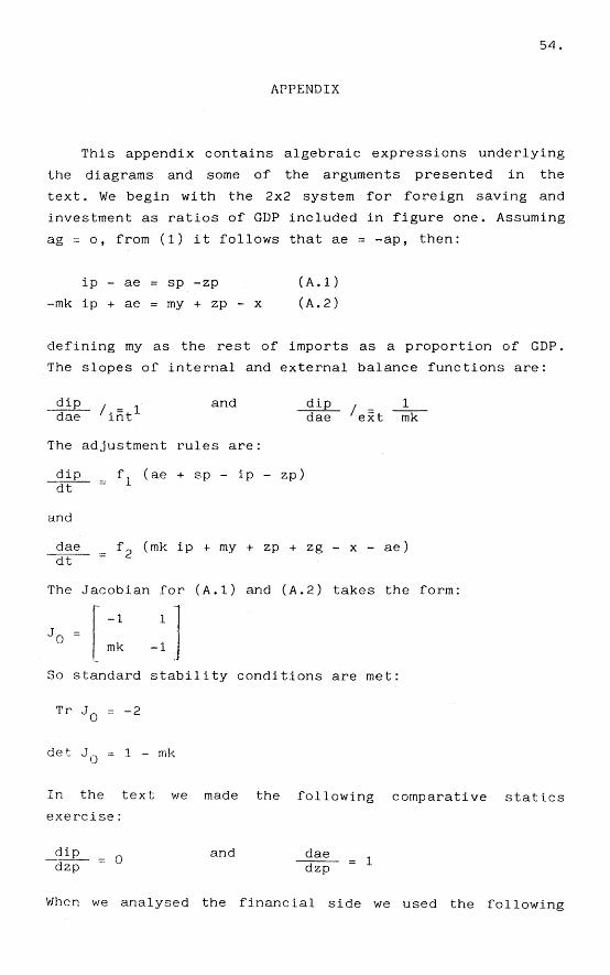
54.

APPENDIX

This appendix contains algebraic expressions underlying

the diagrams and some of the arguments presented in the

text. We begin with the 2x2 system for foreign saving and

investment as ratios of GDP included in figure one. Assuming

ag = o, from (1) it follows that ae = -ap, then:

ip - ae = sp -zp (A.l)

-mk ip + ae = my + zp - x (A.2)

defining my as the rest of imports as a proportion of GDP.

The slopes of internal and external balance functions are:

dip i - \ a n d dip / _ 1 dae int dae 'ext mk

The adjustment rules are:

dip f (ae + sp - ip - zp) dt =

and

dae _ fp (mk ip + my + zp + zg - x - ae) dt

The Jacobian for (A.l) and (A.2) takes the form:

-1 1

mk -1

So standard stability conditions are met:

Tr JQ = -2

det J = 1 - mk

In the text we made the following comparative statics

exercise:

dip _ 0 and dae _ 1 dzp dzp

When we analysed the financial side we used the following

55.

model:

ip - sp + Anf = -zp (A.3)

-mk ip = ink ig + my + zg + zp - x - 4k - ̂ r (A.4)

Anf = -Ak + Ar + Acg (A.5)

The right-hand side variables are all exogenous and

ip = ip (q; rm)

Anf = nf (q; rm)

Acg = g + zg + ig - t

with:

9 i p i p q > 0 3Q

3 i p i p r < 0

" m

dAnf nfq < 0 aq -

9Anf n f r > 0 9 r ° m

Where r s

(A.6)

(A.7)

(A.8)

(A.9)

t a n d s fo stands for the interest rate of financial m assets and q stands for the demand price of capital goods.

This variable should be interpreted in the Minsky sense.

That is, it represents the price which capitalists are

prepared to pay for capital goods and not necessarily the

actual price of capital goods on the market.

The adjustment rules are:

dsp _ f (ip + Anf + zp - sp) dt ~

dq _ f (4k + x - mk ip - my - zp - zg - Ar) dt q

dr f J}] r (Av + g + zg + ig - Anf - t - Ak)

dt " m

The Jacobian for (A.3), (A.4), and (A.5) takes the form:

56.

-1 ipq + nfq ipr + nfr

-mk ipq -mk ipr

0 -nfq -nfr

And the stability conditions are the following:

(1) Tr JL = -1 - mk ipq - nfr<0, which is true given that

the signs of (A.6), (A.9), and mk are all positive.

(2) det J. = mk (nfq ipr - ipq nfr)<0, wnich is met if we

assume that the assets are gross substitutes.

(3) mk (ipq nfr - nfq ipr)> 0, which is met if (2) is true

nfr>0, which is true given the assumption made in (A.9)

mk ipq>0, which is true given (A.6).

These are the algebraic equations relevant to the

comparative statics exercises in the text; first an

increment of zp:

dsp _ 1-mk .n dzp ~ mk

dq nfr dzp dr m

dzp

detJ 1

nfq detJ.

<0

<0

and, second, an increase of zg:

dsp 1-mk dzg mk <0

dq _ nfr + mk ipr , n dzp ~ detJ.

dr , _ m _ -mk ipq -nfq v n

detJ1 > u dzp

57.

FOOTNOTES

1. For a detailed analysis of the economic policies implemented during 1975-84 see Canitrot (1981), Fanelli y Frenkel (1985b), Feldman y Sommer (1983) and Frenkel (1980a). For 1964-74 see Mallon y Sorrouille (1975) and Williamson (1983). Frenkel (1983a) and Winograd (1984) examine the internal consistency of the 'active crawling peg' policy.

2. This estimation is based on Fanelli y Frenkel (1985a).

3. Regrettably no data are available on income distribution.

4. For an examination of the evolution of the domestic financial market during the 'active crawling peg' policy and the financial liberalization see Damill y Frenkel (1985) and Fanelli (1984).

5. The formalization in relation to the real side of the economy follows partially Taylor (1983) and Bacha (1983).

6. See, among others, Diaz Alejandro (1963), Canitrot (1975), Canitrot y Rozenwurcel (1984) and Sidrauski (1968).

7. See, for example, Krugman and Taylor (1978).

8. 2.4 per cent of GDP in 1984.

9. 4.3 per cent of GDP in 1984.

10. mk averaged 10.5 per cent in the last years. For the model see eq. (A.l) and (A.2) in the Appendix.

11. See McKinnon (1973) and Shaw (1973). In 1977 a financial reform was implemented which followed the 'financial liberalization' paradigm to the letter. Interest rates were freed and quantitative constraints on credit eliminated.

12. 'Notional' in the 'clower' sense. See Clower (1965), Leijonhufvud (1968) or Benassy (1982).

58.

13. See for example Tobin (1969).

14. See Tobin (1982) or Taylor and Rosensweig (1984). Damill and Fanelli (1986) develop a less aggregated financial matrix for Argentina taking into account the effects of capital gains and losses due to changes in relative asset prices.

15. We are ignoring here the financial adjustment within the private sector. If, as a consequence of falling investment (ie falling sales), debtors' liquidity worsens, financial fragility will grow and the interest rate will increase. For the concepts of 'financial fragility1 and 'demand price of capital goods', see Minsky (1975). For the model see the second model in the appendix.

16. The conclusion, then, is that there is an inverse relationship between fiscal deficit and investment. However, this should not be interpreted as a simple crowding out argument, because we are not assuming that output is fixed. We are only trying to explain what happens with investment/output ratio, that is - given the capital/output ratio - what happens to the potential rate of growth of the economy in the medium run. The model is not aimed at explaining the level of short-run activity because its main purpose is to stress the trade off between payments on outstanding foreign debt and the potential growth rate.

Nonetheless, we want to stress here the difference between our rationale of the adjustment of the economy and the crowding out argument. The latter says that, assuming full employment, if the government increases public expenditures (either of consumption or of capital goods), private investment would fall because of the increase in interest rates caused by this action. In principle, output could remain constant because the increase in public expenditure would roughly offset the decrease in investment. In our model, on the contrary, the fiscal gap worsens because of the increases in interest payments on outstanding foreign debt. That is, the government borrows funds from the market but the government does not spend such funds on goods. As a consequence, effective demand cannot remain constant. At the same time, since our framework is the two-gap model (with rationing in the international credit market) output should not be constant as long as the main tool for generating an external surplus in the short run is to provoke a decline in imports of both intermediate and capital goods. Given that my and mk are constant, not only investment but output has to decline. In order to maintain a manipulable model we emphasize here the effect of higher interest payments on investment. But there is also a trade-off between interest payments and

59.

activity level in the short run.

17. The main justification for this assumption is that, in the context of high inflation, the growth of output is small in comparison to price changes. So, for the sake of simplifying the algebra, g. can be ignored. This should not be interpreted as a 'full employment' assumption. On the other hand, we are only discussing identities here. We are not saying that inflation does not influence aggregate demand. It is obvious that an acceleration of inflation would cause a contraction in demand because of the increment in the 'inflationary tax' paid by the private sector. However, this last effect might be offset by the Fisher effect. That is, in any economy there are not only 'external' assets issued by the government but also 'inside' assets issued by banks and firms. In this sense Tobin (1980) is very clear, he says 'aggregation (of financial assets and liabilities) would not matter if we could be sure that the marginal propensities to spend from wealth were the same for creditors and debtors. But if the spending propensity were systematically greater for debtors, even by a small amount, the Pigou effect would be swamped by the Fisher Effect' (p. 10). The Argentine experience in 1982 was that the acceleration of inflation provoked a fall in private (and public) debt that led to output expansion. Nonetheless, the relation between changes in inflation and effective demand depend heavily on the economic context. To be specific, it is very important to know if nominal interest rates adjust to the increase in inflation or not.

18. Damill and Fanelli (1986) develop a methodology for a correct measure of the inflationary tax that differs from Cagan (1956) and Friedman (1971).

19. To the extent that the reserve requirement was almost 100 per cent during the last years. M practically does not generate credit to the private sector. In 1983, on the other hand, lt = 3.8 per cent and the inflationary tax paid averaged 5.86 per cent of the GDP. In 1984 1. maintained its level, but the inflationary tax paid averaged 6.9 per cent of the GDP.

20. For a more detailed discussion of this concepts see Damill and Fanelli (1986).

21. For example, in 1984, ex post:

Zll, = 0.4 per cent

—— = 6.5 per cent Pt Yt

60.

a n d 1. - 1 — £ — =6.9 per cent z-i i+ t

This calculation was made following the methodology proposed by Damill and Fanelli (1986).

22. This dilemma appears here because of our assumption that the monetary base is the only financial asset in the economy. In fact, the government could create new government liabilities to avoid this problem. However, this alternative would put high pressure on domestic interest rates as we have seen before. Another alternative that the government usually employs is that of incurring in arrears ('atrasos de tesoreria') and thus forcing the private sector to hold financial assets. This is a disequilibrium solution to the problem in the sense that ex post the private sector would have undesired financial assets in an amount equal to the quantity of arrears. This solution would also provoke a rise in the interest rate.

23. A model closely related to the present one is described in Taylor (1979), chapter 9. Taylor follows Cauas' line of work. We thank Lance Taylor for this reference.

24. For a review of Latin American structural theory of inflation, see Figueiredo et al (1985).

25. Here we follow Frenkel (1983b) and (1984a).

26. Good references on the microeconomic rationale for mark up pricing are Kalecki (1971), Okun (1981) and (for high inflation) Frenkel (1979).

27. Indeed, the mark up rate depends on expected capital losses and expected income losses. See Frenkel (1979).

61.

REFERENCES

Bacha, Edward L. (1983) 'Growth with Limited Supplies of Foreign Exchange: A Reappraisal of the Two Gap Model', Pontifical Catholic University.

Benassy, Jan Pascal (1982) The Economics of Market Disequilibrium, Academic Press.

Cagan, P. (1956) 'The Monetary Dynamics of Hyperinflation', in Friedman (ed.), Studies in the Quantity Theory of Money, Chicago University Press.

Canitrot, Adolfo (1975) 'La experiencia populista de redistribucion de ingresos', Desarrollo Eccnomico, N 59.

Canitrot, Adolfo (1981) 'Teoria y practica del liberalismo. Politica anti-inflacionaria y apertura economica en la Argentina', Desarrollo Economico, N82.

Canitrot, Adolfo y Rozenwurcel, Guillermo (1984) 'El papel de la relacion entre el tipo de cambio y los salarios en una economia semi-industrializada', Buenos Aires, CEDES, Mimeo.

Clower, R. W. (1965) 'The Keynesian conterrevolution: a theoretical appraisal*, in The Theory of Interest Rates, Hahn, F. H. and Brechling, P. R. (eds.), Macmillan.

Damill, M. y Fanelli, J. M. (1986) 'Un Modelo para el analisis del Sistema Financiero y el Deficit Fiscal', Buenos Aires, CEDES, Mimeo.

Damill, M. y Frenkel, R. (1985) 'De la Apertura a la Crisis Financiera. Un Analisis de la Experiencia Argentina de 1977-82', Ensayos Economicos, Forthcoming.

Diaz Alejandro, Carlos F. (1963) 'A note on the impact of devaluation and distributive effect', Journal of Political Economy, N°71.

Fanelli, Jose Maria (1984) 'Ahorro, inversion y financiamiento. Una vision macroeconomica de la experiencia argentina', Ensayos Economicos, N°31.

62.

Fanelli, J. M. y Frenkel, R. (1985a) 'La deuda externa argentina: un caso de endeudamiento forzado', PES. Politica, Economia y Sociedad, N 1.

Fanelli, J. M. y Frenkel, R. (1985b) 'La Argentina y el Fondo en la ultima decada', SELA, Forthcoming.

Feldman E. y Sommer, J. (1983) Crisis Financiera y Endeudamiento Externo, CET/IPAL.

Figueiredo, J. et al. (1985) Empleo y Salarios en America Latina, ECIEL.

Frenkel, Roberto (1979) Decisiones de precio en alta Inflacion, Buenos Aires, Estudios CEDES.

Frenkel, Roberto (1980) Las recientes politicas de estabilizacion en la Argentina: de la vieja a la nueva ortodoxia, PUC/RJ\

Frenkel, Roberto (1983a) 'Mercado financiero, expectativas cambiarias y movimiento de capitales', El Trimestre Economico, N 200.

Frenkel, Roberto (1983b) La dinamica de los precios industriales en la Argentina, 1966-1982. Un estudio econometrico. Buenos Aires, Estudios CEDES.

Frenkel, Roberto (1984) 'Salarios industriales e inflacion. El periodo 1976-1982', Desarrollo Economico, N°95.

Friedman, Milton (1971) 'Government Revenue from Inflation', Journal of Political Economy, July, August.

Kalecki, Michal (1971) "Cost and Prices' and Distribution of National Income', in Selected Essays on the Dynamics of the Capitalist Economy, Cambridge University Press.

Krugman, P. y Taylor, L. (1978) 'Contractionary Effects of Devaluation', Journal of International Economics, N°8.

Leijonhufvud, A. (1968) On Keynesian economics and the economics of Keynes, Oxford University Press.

63.

Mallon, R. y Sourrouille, J. (1975) La politica economica en una sociedad conflictiva: El caso argentino, Buenos Aires, Amorrortu.

McKinnon, Ronald I. (1973) Money and Capital in Economic Development, The Brookings Institution.

Minsky, Hyman (1975) John Maynard Keynes, Columbia University Press.

Okun, Arthur (1981) Prices and Quantities. A Macroeconomic Analysis, The Brookings Institution.

Shaw, Edward (1973) Financial Deepening in Economic Development, Oxford University Press.

Sidrauski, Miguel (1968) 'Devaluacion, inflacion y desempleo', Economica, Vol. 14, Jan.Aug.

Taylor, Lance (1979) Macromodels for developing countries, Mc Graw Hill.

Taylor, Lance (1983) Structuralist Macroeconomics, Basic Books.

Taylor, Lance and Rosenweig, J. A. (1984) 'Devaluation, Capital Flows, and Crowding Out. A Computable General Equilibrium Model with Portfolio Choice for Thailand1, MIT, Mimeo.

Tobin, James (1969) 'A General Equilibrium Approach to Monetary Theory', Journal of Money, Credit and Banking, N 1. ~~

Tobin, James (1980) Asset accumulation and economic Activity, Basil Blackwell.

Tobin, James (1981) 'Money and Finance in the Macroeconomic Process', Journal of Money, Credit and Banking, N°14.

Williamson, John (ed.) (1983) IMF Condicionality, MIT Press.

Winograd, Carlos (1984) Economia abierta y tipo de cambio prefijado. j Que aprendemos del caso argentino? Estudios CEDES.

64.

Table 1

MACROECONOMIC INDICATORS

1965-74

J 975-84

197C

197]

1972

1973

1974

1975

1976

1977

1976

1979

1980 1981

1962

19B3

1-984

GDP Growth Rate

(1)

4,4

0,4

4.5

3.7

1,9

3,4

5,7

-0,4

-0,5

6,4

-2,9

6,2

0,8

-6,2

-5,1

3,1

2.4

Inflation Rate (CPI)

(2)

30,5

247,9

13,6

34,9

58,4

60,3

24,2

182,8

444,1

176,0

175,5

159,5

100,8

104,5

164,6

343,8

626,7

Real Exchange Rate (3)

(a)

99,8

105,4

101,6

90,2

106,6

100,0

109,4

112,6

142,6

119,9

95,e

68,6

53, C

68,7

121,e

141,1

126,7

(b)

90,9

93,8

100,5

91,5

101 ,1

100,0

104,7

88,9

110,3

110,6

95,6

72,1

61,3

75,9

103,9

109,5

109,6-

Real Wage

(4)

97,4

84,8

95,5

99,0

94,1

100,0

113,1

105,5

71,2

71,9

69.3

79,8

86,7

80,5

71,7

94,5

114,9

Balance of Payment6 (5)

Trade Account

269,1

1166,5

79,1

-127,7

36,4

1036,5

295,8

-985,2

883,1

1490,3

2565,8

1109,9

-2519,2

-287,0

2286,8

3320,0

3800,0

Current Account

35,7

-1481,5

-158,9

-388,7

-222,9

720,7

f*r,Z

-1284,6

649,6

1289,9

1833,6

-536,4

-4767.8

-4714,0

-2657,7

-2437,5

-2190,0

Nomina! . Net

External Debt

(6)

na

na

na

3948,0

5359,0

7256,0

6467,0

5639,0

6<f«"9,0

8554,0

19478,0

31794,0

37477,0

40907,0

44155,0

(?• - a) Deflator Domestic Prices : Consumer Price Index (CPI) (3 - b) Deflator Doestic Prices : Knolesale Industrial Prices Net of Foodstuf (3) and (4) Index 1973. «= 100 (5) and (6) In Millions of Dollars (7) As % of GDP

Sources : Based on Central Bank, Secretary of Finance and Indec.

Table 2

COMPOSITION OF OUTPUT AND RATES OF GROWTH

196J-74*

1975-84*

1970

1971

1972

1973

1974

1975

1976

1977

1978

1979

1980

1981

1982

1983

1984

-

Total GDP

A.G.

4,4

0,4

4,5

3,7

1,9

3,5

5,7

-0,4

-0,5

6,4

-2,9

6,2

0,8

-6,2

-5,1

3,1

2,4

(c)

100,0

100,0

100,0

100,0

100,0

100,0

100,0

100,0

100,0

100,0

100,0

100,0

100,0

100,0

100,0

100,0

100,0

Agriculture

A.G.

2,7

1,8

4,8

1,6

1,9

10,7

2,7

-2,8

4,5

2,5

2,8

3,5

-6,7

2,4

7,3

0,9

3,5

(c)

13,0

14,1

13,2

12,9

12,9

. 13,8

13,4

13,1

13,7

13,3

14,1

13,7

12,7

13,8

15,6

15,3

15,5

Mining

A.G.

5,8

2,6

5,1

7,8

2,9

-2,8 2»4

-1,5

2,4

8,5

1,9

6,3

5,8

0,6

-0,7

2,2

0,3

(c)

2.1.

2,5

2,3

2,4

2,4

2,3

2,2

2,2

2,2

2,3

2,4

2,4

2,5

2,7

2,8

2,8

2,7

Industry

A.G.

5,7

-0,7

4,2

6,1

4,0

4,0

5,9

-2,6

-3,0

7,8

-10,5

10,2

-3,8

-16,0

-4,7

10,8

4,4

<c)

31,1

25,5

27,0

27,6

28,2

28,3

28,4

27,8

27,0

27,4

25,4

26,2

25,0

22,4

24,5

24,2

24,7

Elect.

A.G.

9,1

5,3

10,7

9,3

9,9

7,5

6,0

6,1

3,7

4,6

3,3

10,7

7,8

-1,1

3,1

8,0

6,8

& Water

(c)

2,4

3,6

2,3

2,5

2,6

2,8

2,8

2,9

3,1

3,0

3,2

3,3

3,6

3,8

4,1

4,3

4,5

Construction

A.G.

7,2

-3,4

13,8

6,3

-1,0

-11,7

7,9

4,6

14,9

12,1

-4,7

-0,5

1,2

-13,8

-19,8

-6,8

-20,9

(c)

5,1

6,0

6,5

6,6

6,4

5,5

5,6

5,9

6,8

7,2

7,1

6,6

6,6

6,1 5»J

4,7

3,6

Services

A.G.

3,7

0,7

3,0

2,2

0,7

3,3

6,3

0,5

-2,4

5,9

-1,4

6,6

4,6

-3,2

-7,7

0,9

2,9

(c)

46,3

48,4

48,7

48,0

47,5

47,3

47,6

48,1

47,2

46,8

47,8

47,8

49,6

51,2

47,9

48,7

49,0

A.G. : Annual Rate of Growth, (c) : % of GDP * : Average Rate of Growth.

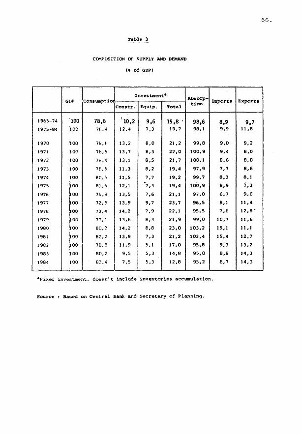
66.

Table 3

COMPOSITION OF SUPPLY AND DEMAND

(% of GDP)

1 9 6 5 - 7 4

1 9 7 5 - 8 4

1970

1971

1972

1973

1974

1975

1976

1977

1976

1979

1980

1981

1982

1983

1984

GDP

100 100

ioo 100

100

100

100

boo 1 Si o o

koo 300

a oo 3 00

jioo J 00

3 00

100

Consumptior

78,8 7f.. 4

7 8 , (•

7 8 , 9

7 6 , 4

7 8 , 5

8 0 . r.

8 1 . r>

7 5 , 9

7 2 , 8

7 3 , 4

7 7 , 1

8 0 , 2

8 2 , 2

7 8 , 8

8 0 , 2

8 2 , 4

I n v e s t m e n t *

C o n s t r .

' l0 ,2 1 2 , 4

1 3 , 2

1 3 , 7

1 3 , 1

1 1 , 3

1 1 , 5

1 2 , 1

1 3 , 5

1 3 , 9

1 4 , 2

1 3 , 6

1 4 , 2

1 3 , 9

1 1 , 9

9 , 5

7 , 5

E q u i p .

9.6 7 , 3

8 , 0

8 , 3

8 , 5

8 , 2

7 , 7

*7,3

7 , 6

9 , 7

7 , 9

8 , 3

8 , 8

7 , 3

5 , 1

5 , 3

5 , 3

T o t a l

19,8 ' 1 9 , 7

2 1 , 2

2 2 , 0

2 1 , 7

1 9 . 4

1 9 , 2

1 9 , 4

2 1 , 1

2 3 , 7

2 2 , 1

2 1 , 9

2 3 , 0

2 1 , 2

1 7 , 0

1 4 , 8

1 2 , 8

A b s o r p ­t i o n

98,6 9 8 , 1

9 9 , 8

1 0 0 , 9

1 0 0 , 1

9 7 , 9

9 9 , 7

1 0 0 , 9

9 7 , 0

9 6 , 5

9 5 , 5

9 9 , 0

1 0 3 , 2

1 0 3 , 4

9 5 , 8

9 5 , 0

9 5 , 2

Imports

8,9 9 , 9

9 , 0

9 , 4

8 , 6

7 , 7

8 , 3

8 , 9

6 , 7

8 , 1

7 , 6

1 0 , 7

1 5 , 1

1 5 , 4

9 . 3

8 , 8

8 , 7

E x p o r t s

9,7 1 1 , 8

9 , 2

8 , 0

8 , 0

8 , 6

8 , 1

7 , 3

9 , 6

1 1 , 4

1 2 , B "

1 1 , 6

1 1 , 1

1 2 , 7

1 3 , 2

1 4 , 3

1 4 , 3

'Fixed investment, doesn't include inventories accumulation.

Source : Based on Central Bank and Secretary of Planning.

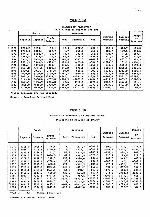
6 7 .

T a b l e 4 (a )

BALANCE OF PAYMENTS-

( In M i l l i o n s o f c u r r e n t D o l l a r s )

1970 1971 1972 1 9 7 3 1974 1 9 7 5 1976 1977 1978 1979 1980 1961 1982 1982 1984

Goods

E x p o r t s

1 7 7 3 , 2 1 7 4 0 , 4 1 9 4 1 , 1 3 2 6 6 , 0 3 9 3 0 , 7 2 9 6 1 , 3 3 9 1 6 , 1 5 6 5 1 , 8 6 3 9 9 , 5 7 8 0 9 , 9 8 0 2 1 , 4 9 3 4 3 , 0 7 6 2 3 , 7 7 e 3 5 , 0 8 1 0 0 , 0

I m p o r t s

1 6 9 4 , 1 1 8 6 8 , 1 1 9 0 4 , 7 2 2 2 9 . 5 3 6 3 4 , 9 3 9 4 6 , 5 3 0 3 3 , 0 4 .161,5 3 8 3 3 , 7 6 7 0 0 , 0

1 0 5 4 0 , 6 9 4 3 0 , 0 5 3 3 6 , 9 4 5 1 5 , 0 4 6 0 0 , 0

Trade B a l a n c e

7 9 , 1 - 1 2 7 , 7

3 6 , 4 1 0 3 6 , 5

2 9 5 , 8 - 9 8 5 , 2

8 8 3 , 1 1 4 9 0 , 3 2 5 6 5 , 8 1 1 0 9 , 9

- 2 5 1 9 , 2 - 2 8 7 , 0 2 2 8 6 , 8 3 3 2 0 , 0 3 5 0 0 , 0

S e r v i c e s

Real

- 1 2 , 3 1 ,7

7 8 , 3 6 7 , 9

1 6 4 , 4 1 2 5 , 6 2 4 0 , 5 3 4 6 , 8 - 9 9 , 8

- 7 6 ) , 3 - 7 4 0 , 1 - ? 0 4 , 9

4 2 , 5 - 3 6 5 , 0 - 2 8 3 , 0

F i n a n c i a l

- 2 2 2 , 5 - 2 5 5 , 9 - 3 3 3 , 6 - 3 9 4 , 4 - 3 3 3 , 3 - 4 2 9 , 6 - 4 9 2 , 5 - 5 7 8 , 5 - 6 8 0 , 8 - 9 2 0 , 0

- 1 5 3 1 , 4 - 3 6 9 9 , 7 - 4 7 1 8 , 5 - 5 4 0 7 , 9 - 5 7 1 2 , 0

Net

- 2 3 4 , 6 - 2 5 7 , 6 - 2 5 5 , 3 - 3 2 6 , 5 - 1 6 8 , 9 - 3 0 4 , 0 - 2 5 2 , 0 - 2 3 1 , 7 - 7 8 0 , 6

- 1 6 8 1 , 3 - 2 2 7 1 , 5 - 4 4 0 4 , 6 - 4 6 7 6 , 0 - 5 7 7 2 , 9 - 5 9 9 5 , 0

C u r r e n t A c c o u n t

- 1 5 8 , 9 - 3 8 8 , 7 - 2 2 2 , 9

7 2 0 , 7 1 2 7 , 2

- 1 2 8 4 , 6 6 4 9 , 6

1 2 8 9 , 9 1 8 3 3 , 6 - 5 3 6 , 4

- 4 7 6 7 , 6 - 4 7 1 4 , 0 - 2 3 5 7 , 7 - 2 4 3 7 , 5 - 2 4 9 2 , 1

C a p ! t a l Account

4 1 3 , 7 - 1 8 9 , 5

- 7 4 , 5 1 5 , 0

- 5 3 , 7 1 9 1 , 1

- 5 1 5 . 9 1 2 8 6 , 5 1 3 3 3 , 9 4 6 S 6 . 9 2 5 5 1 , 7 1 4 8 9 , 7

- 2 3 2 3 , 5 - 1 4 0 3 , 0

6 8 4 , 3

— — — — — i

Change i n

R e s e r v e s

1 8 5 , 0 - 3 8 4 , 6

1 6 7 , 1 9 2 1 , 0 - 5 1 , 3

- 7 9 1 , 1 1 1 9 2 , 4 2 2 2 6 , 5 1 9 9 8 , 4 4 4 4 2 , 4

- 2 7 9 6 , 1 - 3 8 0 6 , 5

- 6 5 1 , 1 2 4 3 , 7 1 9 6 , 0

•Minor a c c o u n t s a r e n o t i n l u d e d .

S o u r c e : Based on C e n t r a l Bank

T a b l e 4 (b)

BALANCE OF PAYMENTS IN CONSTANT VALUE

( M i l l i o n s o f D o l l a r s o f 1 9 7 3 ) *

1970 1971 1972 1973 1974 1975 1976 1977 1976 1 9 7 9 1 9 8 0 1 9 6 !

, 1 9 6 2 : i 9 e 3 1984

1

Goods

E x p o r t s

2 1 6 5 , 0 2 0 5 4 , 7 2 1 9 5 , 8 3 2 6 6 , 0 3 3 0 8 , 0 2 2 7 9 , 7 2 8 6 3 , 7 3 9 1 9 , 4 4 1 1 8 , 1 4 4 6 5 , 3 4 0 2 0 , 7 4 2 0 3 , 7 3 4 3 1 , 1 3 4 8 1 , 2 3 5 1 2 , 5

I m p o r t s

2 0 6 8 , 4 2 2 0 5 , 5 2 1 5 4 , 6 2 2 2 9 , 5 3 0 5 9 , 7 3 0 3 8 , 1 2 2 3 2 , 9 2 8 8 5 , 9 2 4 6 7 , 0 3 8 3 7 , 3 5 2 8 3 , 5 4 3 3 5 , 7 2 4 0 1 , 9 2 0 0 6 , 1 1 9 9 4 , 7

Trade B a l a n c e

9 6 , 6 - 1 5 0 , 8

4 1 , 2 1 0 3 6 , 5

2 4 8 , 3 - 7 5 6 , 4

6 5 0 , 8 1 0 3 3 , 5 1 6 5 1 , 1

6 2 8 , 0 - 1 2 6 2 , 8

- 1 3 2 , 0 1 0 2 9 , 2 1 4 7 5 , 1 1 6 4 7 , 6

S e r v i c e s

Rea l

- 1 5 , 0 2 , 0

8 8 , 6 6 7 , 9

1 3 6 , 4 9 6 , 7

1 7 7 , 1 2 4 0 , 5 - 6 4 , 2

- 4 3 6 , 5 - 3 7 1 , 0 - 3 2 4 , 1

1 9 , 1 - 1 6 2 , 2 - 1 2 2 , 7

F i n a n c i a l

- 2 7 1 , 7 - 3 0 2 , 1 - 3 7 7 , 4 - 3 9 * , 4 - 2 8 0 , 6 - 3 3 0 , 7 - 3 6 2 , 7 - 4 0 1 , 2 - 4 3 8 , 1 - 5 2 6 , 0 - 7 6 7 , 6

- 1 7 0 1 , 1 - 2 1 2 3 , 5 - 2 4 0 2 , 8 - 2 4 7 7 , 0

N e t

- 2 8 6 , 7 - 3 0 4 , 1 - 2 8 8 , 1 - 3 2 6 , 5 - 1 4 2 , 2 - 2 3 4 , 0 - 1 8 5 , 6 - 1 6 0 , 7 - 5 0 2 , 3 - 9 6 2 , 5

- 1 1 3 8 , 6 - 2 0 2 5 , 2 - 2 1 0 4 , 4 - 2 5 6 5 , 0 - 2 5 9 9 , 7

C u r r e n t

A c c o u n t

- 1 9 4 , 0 - 4 5 6 , 9 - 2 5 2 , 1

7 2 0 , 7 1 0 7 , 0

- 9 8 8 , 9 4 7 8 , 4 8 9 4 , 5

1 1 7 9 , 9 - 3 1 4 , 5

- 2 3 8 9 , 9 - 2 1 6 7 , 3 - 1 0 6 1 , 0 - 1 0 8 3 , 0 - 1 0 8 0 , 7

C a p i t a l

A c c o u n t

5 0 5 , 1 - 2 2 3 , 7

- 8 4 , 3 1 5 , 0

- 4 5 , 2 1 4 7 , 1

- 3 8 0 , 1 8 9 2 , 2 8 5 8 , 3

2 7 0 2 , 2 1 2 7 9 , 1

6 8 5 , 0 1 0 4 5 , 6 - 6 2 3 , 4

2 9 6 , 7

Change

i n

R s e r v e s

2 2 5 , 8 - 4 5 4 , 0

1 8 9 , 0 9 2 1 , 0 - 4 3 , 1

- 6 0 9 , 1 8 7 8 , 7

1 5 4 4 , 5 1 2 8 5 , 5 2 5 3 9 , 5

- 1 4 0 1 , 7 - 1 7 4 9 , 9

- 2 9 3 , 0 1 0 8 , 3

8 4 , 9

• D e f l a t o r *>-S. *'«wt£i»u£ vace. »vn>e*

S o u r c e : Based on C e n t r a l Bank

Table 5

BALANCE OF EXTERNAL INDEBTNESS ANO SOLVENCY INDICATORS

1973

1974

1975

1976

1977

1978

1979

1980

1981

1982

1983

1984

Public Debt

*

3316

' 4300

4021

5189

6044

8357

9960

14**9

20024

26341

30108

37628

A.G

29,6

-6,5

29,0

16,4

38,2

19,1

45,1

38,4

31,5

14,5

25,0

Private Debt

*

2094

2470

385.4

3090

3634

4139

9074

12703

15647

14362

14269

10193

A.G

17,9

56,0

-19,9

17,6

13,8

119,2

39,9

23,1

-8,3

-0,7

-28,6

(1)

Total Debt

*

5410

6770

7875

8279

9678

12496

19034

27162

35671

40703

44377

47821

A.G

25,1

?6,3

5,1

16,8

29,1

52,3

42,7

31,3

14,1

9,0

7,8

(2)

Reserves

*

1462

1411

619

1812

4039

6037

10480

7684

3877

3226

3470

3666

A.G

-3,5

-56,2

192,7

122,9

49,4

73,5

-26,6

-49,6

-16,8

7,5

5,6

Total Net Debt U)-(2)

*

3948

5359

7256

6467

5639

6459

8554

19478

31794

37477

40907

44155

A.G

35,7

35,3

-10,9

-12,9

14,5

32,4

127,7

63,2

17,8

9,1

7,9

Total Real Net Debt

* «

3948

4510

5587

4671

3912

4155

4890

9764

14616

16866

18176

19147

A.G

14,2

23,8

-16,4

-16,3

6,2

17,6

99,6

49,6

15,3

7,7

5,3

ExportsFinancial Net Services Debt Exports Ratio Ratio

( * ) ( % ) •

82,7

13, h

40,8

61,7

100,1

99,1

91,3

4L1

28,7

20,3

19,1

i§;3

12,0

8,4

14,5

12,5

10,2

10,6

11,7

19,0

40,4

62,5

69,0

70,5

• In Millions of current dollars. ** In Millions of constant dollars of 1973. oi h.Q t Annual rate of growth. J°

69.

Table 6

SOURCES OF EXTERNAL XNDEBTHESS

(in Millions of dollars)

Increase in Net Debt* (i)

Registered Sources**

of Indebtness (2)

Current Account (a)

Trade Credit***

(Exports) (b)

Direct Investment (c)

Parity Adjustment (d)

Unjustified Capital

Flows (e)

Errors and Omissions (f)

Unidentified Debt

Increase (1) - (2)

1976

-788,4

1'386,8

649,6

263,4

-

-16,4

499,2

-9,0

598,4

1977

-827,5

-1035,8

1289,9

255,3

-52,1

9,3

-369,2

-97,4

208,3

1978

819,6

-1738,8

1833,6

8,6

274,2

166,0

-575,9

32,3

2558,4

1979

2095,6

239,8

-536,4

840,8

264,6

132,0

-1142,7

201,9

1855,8

1980

10924,1

9180,3

-4767,8

-33,0

787,7

-213,0

-4655,8

-298,4

1743,8

1981

12315,5

9320,8

-4714,0

-1463,0

927,0

-363,0

-3499,0

-208,8

2994,7

1982

5683,0

2892,1

-2357,7

-504,0

257,0

-106,0

107,0

-286,4

2790,9

1976-82

29591.9

17471,6

-8602,8

-631,9

245E,4

-391,1

-9636,4

-667,8

12120,3

* & Total Debt - h Reserves = (1)

* - ( a * b + c + d + e 4 f ) = (2)

*** Exports credit is not included in foreign debt figures.

Source : Based on Central Bank Data.

7 0 .

Table 7

FINANCIAL INVESTMENT AND FOREIGN PAYMENTS (% Of GDP)

1964

1965

1966

1967

1968

1969

1970

1971

1972

1973

1974

1975

1976

1977

1978

1979

1980

1981

1982

1983

1984

ae

-0,5

-1,5

-1,9

-1

0

0,9

0,9

1

0,9

-1,4

0,1

2,5

-0,9

-1,8

-1,6

1,8

5,5

6,8

2,7

3,2

3,2

-ag

5,5

3,2

4,1

1,2

1,4

1,1

1,1

3,8

4,6

6,6

6,9

14,0

9,8

3,2

3,8

3,6

4,3

6,6

3,4

10,8

7.4

ap

6,0

4,7

6

2,2

1,4

0,2

0,2

2,8

3,7

8,0

6,8

11,5

10,7

5,0

5,4

1,8

-1,2

-0,2

-0,7

7,6

4,2

z

0,5

0,4

1,2

1,4

1,4

1,3

1,1

0,4

1.3

1.5

1.2

1,2

1.3

1,3

1,7

1,9

2,1

5,5

7,2

8,2

8,4*

^Estimated Source: Secretary of planning

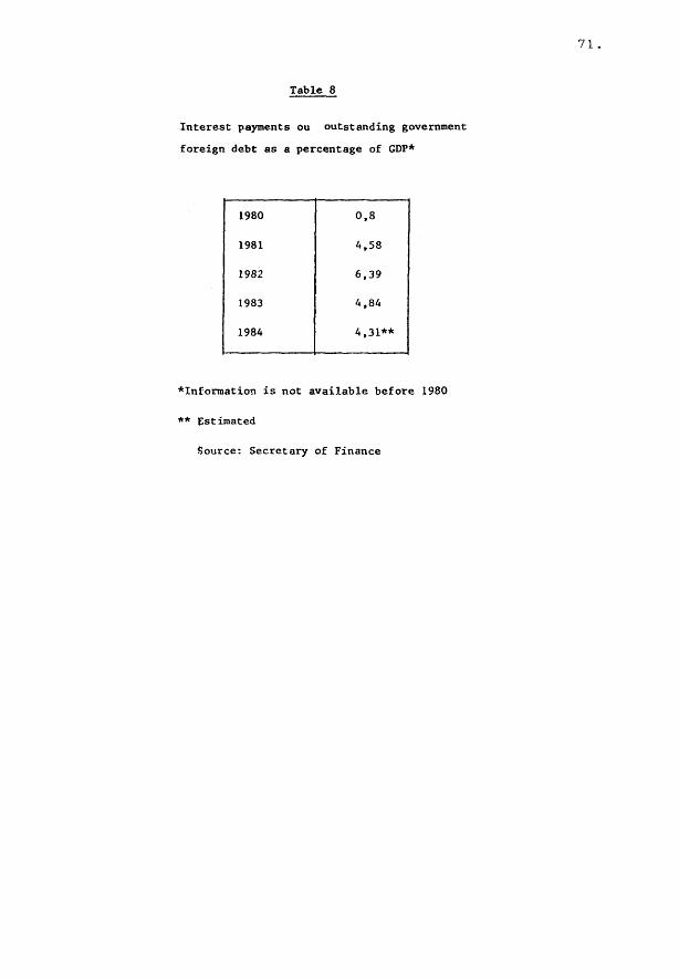
71.

Table 8

Interest payments ou outstanding government

foreign debt as a percentage of GDP*

1980

1981

1982

1983

1984

0,8

4,58

6,39

4,84

4,31**

*Information is not available before 1980

** Estimated

Source: Secretary of Finance

7 2 .

FIGURE ONE

7 3 .

FIGURE TWO

74.

FIGURE THREE