"global pricing of risk and stabilization policies" -- imfs working lunch: tobias adrian
TRANSCRIPT

Global Pricing of Risk and Stabilization Policies
Tobias Adrian Daniel Stackman Erik Vogt
Federal Reserve Bank of New York
The views expressed here are the authors’ and are not necessarily representative of
the views of the Federal Reserve Bank of New York or of the Federal Reserve System
July 2015
T Adrian, D Stackman, E Vogt Global Pricing of Risk July 2015 1
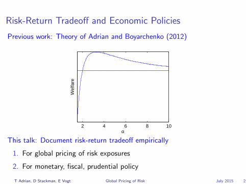
Risk-Return Tradeoff and Economic Policies
Previous work: Theory of Adrian and Boyarchenko (2012)
2 4 6 8 10α
Wel
fare
2 4 6 8 10
0.2
0.4
0.6
0.8
1
α
Dis
tres
s pr
obab
ility
6 month1 year5 year
This talk: Document risk-return tradeoff empirically
1. For global pricing of risk exposures
2. For monetary, fiscal, prudential policy
T Adrian, D Stackman, E Vogt Global Pricing of Risk July 2015 2
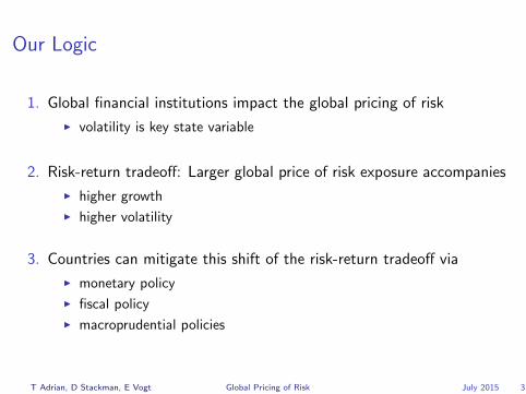
Our Logic
1. Global financial institutions impact the global pricing of risk
I volatility is key state variable
2. Risk-return tradeoff: Larger global price of risk exposure accompanies
I higher growth
I higher volatility
3. Countries can mitigate this shift of the risk-return tradeoff via
I monetary policy
I fiscal policy
I macroprudential policies
T Adrian, D Stackman, E Vogt Global Pricing of Risk July 2015 3

Global Institutions and Global Pricing of Risk
Outline
Global Institutions and Global Pricing of Risk
Global Pricing of Risk and the Macro Risk-Return Tradeoff
The Macro Risk-Return Tradeoff and Economic Policies
T Adrian, D Stackman, E Vogt Global Pricing of Risk July 2015 4

Global Institutions and Global Pricing of Risk
VIX as a Measure of Risk Appetite
I VIX measures global pricing of riskI Global capital flows, credit growth, & asset prices comove with the VIX
(Rey (2015))
I Price of sovereign risk correlates strongly with the VIX
(Longstaff, Pan, Pedersen, and Singleton (2011))
I Nonlinear function of the VIX forecasts stock & bond returns
(Adrian, Crump, and Vogt (2015))
I Monetary policy and the pricing of risk interactI Policy rate reacts to the VIX (Bekaert, Hoerova, and Duca (2013))
I Substantial variation in the VIX attributed to rate shocks
(Miranda-Agrippino and Rey (2014))
I Risk taking channel of monetary policy (Borio and Zhu (2012))
I Why is the VIX so important?
T Adrian, D Stackman, E Vogt Global Pricing of Risk July 2015 5

Global Institutions and Global Pricing of Risk
Global Financial Institutions
I Asset allocation is largely delegated to financial institutions
I The delegation gives rise to principal agents problems
I Contractual features between institution and their investors
I redemptions for asset managers (Vayanos (2004))
I high water marks for hedge funds (Panageas and Westerfield (2009))
I VaR constraints for banks (Adrian and Shin (2014))
I Intermediary constraints tend to correlate with volatility
I In equilibrium, such constraints impact pricing
I intermediary asset pricing He and Krishnamurthy (2008, 2011)
T Adrian, D Stackman, E Vogt Global Pricing of Risk July 2015 6

Global Institutions and Global Pricing of Risk
VaR Constraints of Global Financial Institutions
T Adrian, D Stackman, E Vogt Global Pricing of Risk July 2015 7

Global Institutions and Global Pricing of Risk
Large VIX and Fund Flows
T Adrian, D Stackman, E Vogt Global Pricing of Risk July 2015 8
Global Institutions and Global Pricing of Risk
Institutional Asset Pricing: Theory
Each global financial institution i maximizes
maxnit
Et [nitrt+1]− Covt [n
itrt+1,Xt+1]ψi
t
s.t.VaR it · α ≤ w i
t
Then the demand for each risky asset is:
nit =
1
λitα[Et [rt+1]− Covt [rt+1,Xt+1]ψi
t ][Vart(rt+1)]−1
Market clearing gives equilibrium returns
Et [rt+1] = Covt(rt+1, rMt+1)
1
Σiw it
λitα
+ Covt [rt+1,Xt+1]Σi
w itψ
it
λitα
Σiw it
λitα
T Adrian, D Stackman, E Vogt Global Pricing of Risk July 2015 9

Global Institutions and Global Pricing of Risk
Institutional Asset Pricing: Predictions
Global equilibrium expected returns are:
Et [rt+1] = βtΛt
We assume affine prices of risk:
Λt = λ0 + λ1Xt
Xt =[rMt , r
ft , φ (vixt)
]′φ (vixt) is a nonlinear function of the VIX that is forecasting returns.
T Adrian, D Stackman, E Vogt Global Pricing of Risk July 2015 10
Global Institutions and Global Pricing of Risk
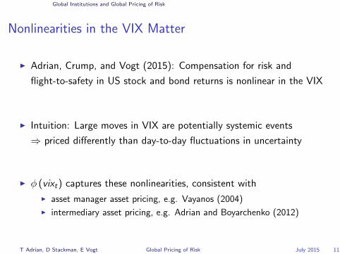
Nonlinearities in the VIX Matter
I Adrian, Crump, and Vogt (2015): Compensation for risk and
flight-to-safety in US stock and bond returns is nonlinear in the VIX
I Intuition: Large moves in VIX are potentially systemic events
⇒ priced differently than day-to-day fluctuations in uncertainty
I φ (vixt) captures these nonlinearities, consistent with
I asset manager asset pricing, e.g. Vayanos (2004)
I intermediary asset pricing, e.g. Adrian and Boyarchenko (2012)
T Adrian, D Stackman, E Vogt Global Pricing of Risk July 2015 11

Global Institutions and Global Pricing of Risk
Estimation of the VIX Pricing Function
I The global price of risk variable φ (VIXt) is unknown
I Estimate nonparametrically by running a forecasting regressions of
global USD equity and bond returns of 27 countries on lagged VIX +
global market
I Sieve Reduced Rank Regressions (SRRR) of (Adrian, Crump, Vogt)
r ct+h = ac + bcφ (VIXt) + ηct+h, c = 1, . . . , (neqts + nbnds + mkt)
I Each expected asset return is an affine transformation of a common
nonlinear function
I SRRR advantage: all 27 equity and 27 bond returns are jointly
informative about shape of φ(·)
T Adrian, D Stackman, E Vogt Global Pricing of Risk July 2015 12

Global Institutions and Global Pricing of Risk
Conditional Sharpe Ratios of Global Stocks and Bonds
Et
[r ct+h
]= ac + bc φ (VIXt)
T Adrian, D Stackman, E Vogt Global Pricing of Risk July 2015 13

Global Institutions and Global Pricing of Risk
Robustness of the Shape of the Nonlinearity:
φ(v) Separately Estimated for US and Rest-of-the-World
T Adrian, D Stackman, E Vogt Global Pricing of Risk July 2015 14

Global Institutions and Global Pricing of Risk
Global Pricing of Risk
Prices of Risk MKT RF φ(v)
λ1 1.09*** -0.03** -0.49***
Et [rt+h] = β(λ0 + λ1Xt)
State variables Xt = [MKTt ,RFt , φ(vt)]′ are
1. price of risk forecasting variables
2. cross sectional pricing factors
T Adrian, D Stackman, E Vogt Global Pricing of Risk July 2015 15
Global Institutions and Global Pricing of Risk
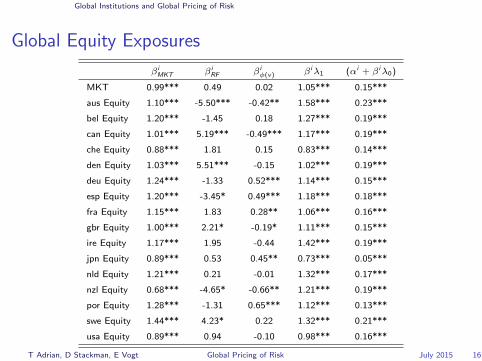
Global Equity Exposures
βiMKT βi
RF βiφ(v) βiλ1 (αi + βiλ0)
MKT 0.99*** 0.49 0.02 1.05*** 0.15***
aus Equity 1.10*** -5.50*** -0.42** 1.58*** 0.23***
bel Equity 1.20*** -1.45 0.18 1.27*** 0.19***
can Equity 1.01*** 5.19*** -0.49*** 1.17*** 0.19***
che Equity 0.88*** 1.81 0.15 0.83*** 0.14***
den Equity 1.03*** 5.51*** -0.15 1.02*** 0.19***
deu Equity 1.24*** -1.33 0.52*** 1.14*** 0.15***
esp Equity 1.20*** -3.45* 0.49*** 1.18*** 0.18***
fra Equity 1.15*** 1.83 0.28** 1.06*** 0.16***
gbr Equity 1.00*** 2.21* -0.19* 1.11*** 0.15***
ire Equity 1.17*** 1.95 -0.44 1.42*** 0.19***
jpn Equity 0.89*** 0.53 0.45** 0.73*** 0.05***
nld Equity 1.21*** 0.21 -0.01 1.32*** 0.17***
nzl Equity 0.68*** -4.65* -0.66** 1.21*** 0.19***
por Equity 1.28*** -1.31 0.65*** 1.12*** 0.13***
swe Equity 1.44*** 4.23* 0.22 1.32*** 0.21***
usa Equity 0.89*** 0.94 -0.10 0.98*** 0.16***
T Adrian, D Stackman, E Vogt Global Pricing of Risk July 2015 16

Global Institutions and Global Pricing of Risk
Global Bond Exposures
βiMKT βi
RF βiφ(v) βiλ1 (αi + βiλ0)
aus Bonds 0.15** -3.05** -0.28* 0.40*** 0.11***
bel Bonds 0.14** -6.66*** 0.09 0.32*** 0.09***
can Bonds 0.12** 0.07 -0.24** 0.25*** 0.09***
che Bonds -0.07 -5.93*** -0.09 0.16* 0.06***
den Bonds 0.07 -5.58*** -0.00 0.25*** 0.08***
deu Bonds 0.04 -6.39*** 0.08 0.21** 0.07***
esp Bonds 0.25*** -8.71*** 0.30* 0.41*** 0.12***
fra Bonds 0.10* -6.95*** 0.12 0.28*** 0.08***
gbr Bonds 0.07 0.38 -0.30 0.20*** 0.08***
ire Bonds 0.08 -5.49*** -0.11 0.32*** 0.10***
jpn Bonds -0.15*** -1.44 -0.09 -0.08 0.00
nld Bonds 0.06 -6.32*** 0.01 0.27*** 0.08***
nzl Bonds 0.16** -4.29** -0.24 0.43*** 0.11***
por Bonds 0.43*** -8.07*** 0.61* 0.44*** 0.12***
swe Bonds 0.17*** -3.25* -0.10 0.34*** 0.10***
usa Bonds -0.23*** -0.03 -0.05 -0.23*** 0.03***
T Adrian, D Stackman, E Vogt Global Pricing of Risk July 2015 17

Global Institutions and Global Pricing of Risk
Institutional Asset Pricing Setup Implies bc = βcλ1
T Adrian, D Stackman, E Vogt Global Pricing of Risk July 2015 18
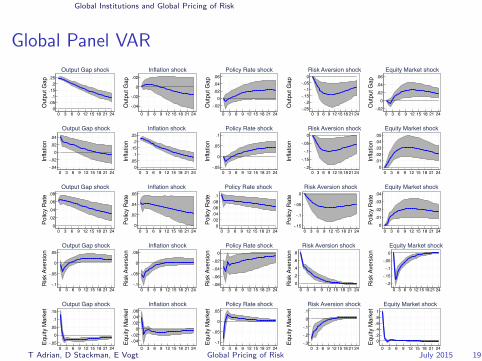
Global Institutions and Global Pricing of Risk
Global Panel VAR
0.05
.1.15
.2.25
Out
put G
ap
0 3 6 9 12 15 18 21 24
Output Gap shock
-.04
-.02
0
.02
Out
put G
ap
0 3 6 9 12 15 18 21 24
Inflation shock
-.020
.02
.04
.06
Out
put G
ap
0 3 6 9 12 15 18 21 24
Policy Rate shock
-.25-.2
-.15-.1
-.050
Out
put G
ap
0 3 6 9 12 15 18 21 24
Risk Aversion shock
-.02
0
.02
.04
.06
Out
put G
ap
0 3 6 9 12 15 18 21 24
Equity Market shock
-.04-.02
0.02.04
Infla
tion
0 3 6 9 12 15 18 21 24
Output Gap shock
0.05
.1.15
.2.25
Infla
tion
0 3 6 9 12 15 18 21 24
Inflation shock
-.05
0
.05
.1
Infla
tion
0 3 6 9 12 15 18 21 24
Policy Rate shock
-.2
-.15
-.1
-.05
0
Infla
tion
0 3 6 9 12 15 18 21 24
Risk Aversion shock
0.01.02.03.04.05
Infla
tion
0 3 6 9 12 15 18 21 24
Equity Market shock
0
.02
.04
.06
.08
Polic
y Ra
te
0 3 6 9 12 15 18 21 24
Output Gap shock
0
.02
.04
.06
Polic
y Ra
te
0 3 6 9 12 15 18 21 24
Inflation shock
0.02.04.06.08
.1
Polic
y Ra
te
0 3 6 9 12 15 18 21 24
Policy Rate shock
-.15
-.1
-.05
0
Polic
y Ra
te
0 3 6 9 12 15 18 21 24
Risk Aversion shock
0
.01
.02
.03
.04
Polic
y Ra
te
0 3 6 9 12 15 18 21 24
Equity Market shock
-.1
-.05
0
.05
Risk
Ave
rsio
n
0 3 6 9 12 15 18 21 24
Output Gap shock
-.1
-.05
0
.05
Risk
Ave
rsio
n
0 3 6 9 12 15 18 21 24
Inflation shock
-.08-.06-.04-.02
0
Risk
Ave
rsio
n
0 3 6 9 12 15 18 21 24
Policy Rate shock
0.2.4.6.8
Risk
Ave
rsio
n0 3 6 9 12 15 18 21 24
Risk Aversion shock
-.2-.15
-.1-.05
0
Risk
Ave
rsio
n
0 3 6 9 12 15 18 21 24
Equity Market shock
-.05
0
.05
.1
.15
Equi
ty M
arke
t
0 3 6 9 12 15 18 21 24
Output Gap shock
-.04-.02
0.02.04.06
Equi
ty M
arke
t
0 3 6 9 12 15 18 21 24
Inflation shock
-.1
-.05
0
.05
Equi
ty M
arke
t
0 3 6 9 12 15 18 21 24
Policy Rate shock
-.3
-.2
-.1
0
.1
Equi
ty M
arke
t
0 3 6 9 12 15 18 21 24
Risk Aversion shock
0.2.4.6.81
Equi
ty M
arke
t
0 3 6 9 12 15 18 21 24
Equity Market shock
T Adrian, D Stackman, E Vogt Global Pricing of Risk July 2015 19

Global Institutions and Global Pricing of Risk
Takeaways from the Global Pricing of Risk
I Theoretically: VaR constraints of global financial institutions give role
to volatility in the pricing of risk
I Empirically: VIX is a strong nonlinear forecasting variable as predicted
by intermediary asset pricing theories
I Consequence 1: Cross country dispersion in the exposure to the
global pricing of risk
I Consequence 2: Shocks to the global pricing of risk forecasts
domestic macro performance
What are the macroeconomic consequences?
T Adrian, D Stackman, E Vogt Global Pricing of Risk July 2015 20

Global Pricing of Risk and the Macro Risk-Return Tradeoff
Outline
Global Institutions and Global Pricing of Risk
Global Pricing of Risk and the Macro Risk-Return Tradeoff
The Macro Risk-Return Tradeoff and Economic Policies
T Adrian, D Stackman, E Vogt Global Pricing of Risk July 2015 21

Global Pricing of Risk and the Macro Risk-Return Tradeoff
Global Bond Exposures and Macro Outcomes
I Exposure b to global pricing of risk varies across countries
I How does it relate to macro outcomes?
I Are countries with higher exposure more volatile?
I Do countries with higher exposure grow faster?
I Are crises more likely?
T Adrian, D Stackman, E Vogt Global Pricing of Risk July 2015 22

Global Pricing of Risk and the Macro Risk-Return Tradeoff
Macroeconomic Outcomes and Global Risk Exposures
T Adrian, D Stackman, E Vogt Global Pricing of Risk July 2015 23

Global Pricing of Risk and the Macro Risk-Return Tradeoff
Cross-Section of Macro and Financial Outcomes
Table 6: The Risk-Return Tradeo↵ in the Cross-Section of Macro and Financial Out-comes
This table reports results from cross-sectional regressions of the indicated outcome variables on globalrisk loadings bi, obtained from sieve reduced rank regressions (SRRR) Et[Rxi
t+h] = ↵i + bi�h(vixt).The index i ranges over the global market excess return (MKT), 27 country stock returns, andcorresponding 27 10-year sovereign bond excess returns in the SRRR estimation. The resulting 27 bi
country stock return loadings and 27 bi bond return loadings form the independent regressors in thetable below. The forecast horizon is h = 6 months, and the sample consists of an unbalanced panelof observations from 1990:1 to 2014:12. All returns are expressed in US dollars.
Panel A: Macro Outcomes Real GDP Inflation
Mean Volatility Mean Volatility
Equities 3.16*** 4.49*** 1.05 1.90Bonds �1.34 �1.91 4.55* 4.87
p-val 0.00 0.00 0.20 0.36R2 0.56 0.55 0.22 0.09Obs 27 27 27 27
Panel B: Banking Outcomes Credit Crisis Output
Boom NPL Pre-Crisis Gain Crisis Loss
Equities 1.14*** 28.38*** 19.81*** 60.58**Bonds 0.21 �12.25 �3.44 �1.18
p-val 0.00 0.00 0.00 0.04R2 0.46 0.41 0.41 0.24Obs 22 22 27 22
Panel C: Financial Market Outcomes Equity Market Bond Market
Mean Downside Volatility Mean Upside Volatility
Equities 0.00 0.30*** 0.25 �0.20Bonds 0.07*** �0.01 5.20*** 0.83**
p-val 0.02 0.00 0.00 0.01R2 0.26 0.74 0.59 0.22Obs 27 27 27 27
12
T Adrian, D Stackman, E Vogt Global Pricing of Risk July 2015 24
Global Pricing of Risk and the Macro Risk-Return Tradeoff
Global Bond Exposures and Economic Policies
I Is aggressiveness of stabilization policies systematically related to
global price of risk exposure?
I Aggressiveness of monetary policy
I Degree of countercyclicality of fiscal policy
I Macroprudential policies
T Adrian, D Stackman, E Vogt Global Pricing of Risk July 2015 25

Global Pricing of Risk and the Macro Risk-Return Tradeoff
Aggressiveness of Stabilization Policies
Table 10: Summary Table: Policy Instruments
This table reports Taylor Rule coe�cient estimates from quarterly regressions of country-specificshort rates on associated output gap and inflation (Ri
f,t = �i0 + �i
outputOGit + �i
inflinflit + "it), along
with sample means of fiscal policy and macroprudential variables used in subsequent tables. Column
(1) reports �ioutput, column (2) �i
infl, and (3) reports���output
i
�� +����infl
i
���. Column (4) reports Mean
ratio of government spending to GDP, and column (5) reports the the degree of countercyclicality offiscal policy, which is proxied by the slope coe�cient from a regression of country i’s output gap ongovernment consumption. Column (6) is the financial sector-targeted macroprudential policy indexas defined in [?].
Taylor Rule Coe�cients Fiscal Policy Variables Macroprudential Index
Mean Gov’t Output Gap - Financial Inst. -
�outputc �infl
c
���outputc
�� +���infl
c
�� Spending/GDP Fiscal Exp. Corr. Targeted
aus �0.42 0.25 0.67 17.81 �1.38*** 1.00bel 0.09** 0.52 0.62 22.40 �0.45*** 2.00can �0.15 1.02*** 1.17 21.09 �0.23*** 3.00che 0.05*** 0.72*** 0.77 10.95 �0.54** 1.57cze 0.06** 0.48*** 0.54 19.93 �0.33** 1.00den 0.22*** 1.21 1.43 25.05 �0.50***
deu 0.40*** 0.67*** 1.07 18.79 �0.61*** 0.57esp �0.17 1.06*** 1.22 18.03 �0.33*** 2.00fin 0.19*** 0.32** 0.51 22.22 �0.51*** 0.07fra 0.13** 1.22*** 1.36 22.64 �0.78*** 2.21gbr 0.09*** 0.75*** 0.84 19.16 �0.22*** 0.00hun 0.00* 0.15*** 0.15 21.35 0.27** 0.50ire �0.04 �0.18* 0.21 16.12 �0.32*** 0.00ita 0.03*** 0.61* 0.65 18.89 �0.70*** 2.00jpn 0.18** 0.69** 0.87 16.70 �0.41*** 1.00kor 0.34*** 0.05*** 0.39 12.30 �0.63*** 0.71mal 0.11*** �0.05 0.16 11.93 �0.44*** 1.00nld 0.28*** 1.31*** 1.59 23.10 �0.25*** 0.14nor 0.43*** 0.46*** 0.89 20.53 �0.21** 1.07nzl 0.05*** 0.13 0.18 17.99 �0.36*** 0.00pol 0.28** 0.67*** 0.95 18.35 �0.58*** 1.00por �0.31 0.24** 0.55 19.39 0.20** 0.50saf �0.65* �0.23 0.89 18.91 0.18 0.07sgp �0.01* �0.17 0.18 9.98 0.08 1.00swe 0.09** 0.84*** 0.92 25.46 �0.13 0.00tha �0.06*** 0.44*** 0.50 13.80 0.24*** 0.21usa 0.18*** 1.54*** 1.72 15.38 �0.71*** 2.93
16
T Adrian, D Stackman, E Vogt Global Pricing of Risk July 2015 26

Global Pricing of Risk and the Macro Risk-Return Tradeoff
Global Risk Exposures and Taylor Rule Coefficients
More aggressive Taylor rule coefficients associated with lower b
T Adrian, D Stackman, E Vogt Global Pricing of Risk July 2015 27
Global Pricing of Risk and the Macro Risk-Return Tradeoff
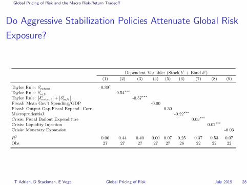
Do Aggressive Stabilization Policies Attenuate Global Risk
Exposure?
Table 7: Global Risk Loadings and Policy Tools
This table reports results from cross-sectional regressions of global risk loadings bi on the indicatedpolicy variables. The global risk loadings bi are obtained from sieve reduced rank regressions (SRRR)Et[Rxi
t+h] = ↵i + bi�h(vixt). The index i ranges over the global market excess return (MKT), 27country stock returns, and corresponding 27 10-year sovereign bond excess returns in the SRRRestimation. The resulting 27 bi country stock return loadings and 27 bi bond return loadings formthe dependent variables in the table below. The forecast horizon is h = 6 months, and the sampleconsists of an unbalanced panel of observations from 1990:1 to 2014:12. All returns are expressed inUS dollars.
Dependent Variable: Stock bi
(1) (2) (3) (4) (5) (6) (7) (8) (9)
Taylor Rule: �ioutput 0.08
Taylor Rule: �iinfl -0.37***
Taylor Rule:���i
output
�� +���i
infl
�� -0.46***
Fiscal: Mean Gov’t Spending/GDP -0.02Fiscal: Output Gap-Fiscal Expend. Corr. 0.12Macroprudential -0.13**
Crisis: Fiscal Bailout Expenditure 0.02***
Crisis: Liquidity Injection 0.01***
Crisis: Monetary Expansion -0.03*
R2 0.00 0.32 0.42 0.07 0.02 0.14 0.50 0.29 0.14Obs 27 27 27 27 27 26 22 22 22
Dependent Variable: Bond bi
(1) (2) (3) (4) (5) (6) (7) (8) (9)
Taylor Rule: �ioutput -0.47***
Taylor Rule: �iinfl -0.18
Taylor Rule:���i
output
�� +���i
infl
�� -0.11Fiscal: Mean Gov’t Spending/GDP 0.02**
Fiscal: Output Gap-Fiscal Expend. Corr. 0.18Macroprudential -0.09*
Crisis: Fiscal Bailout Expenditure 0.00Crisis: Liquidity Injection 0.01***
Crisis: Monetary Expansion 0.00
R2 0.26 0.14 0.05 0.09 0.08 0.12 0.04 0.49 0.00Obs 27 27 27 27 27 26 22 22 22
Dependent Variable: (Stock bi + Bond bi)
(1) (2) (3) (4) (5) (6) (7) (8) (9)
Taylor Rule: �ioutput -0.39*
Taylor Rule: �iinfl -0.54***
Taylor Rule:���i
output
�� +���i
infl
�� -0.57***
Fiscal: Mean Gov’t Spending/GDP -0.00Fiscal: Output Gap-Fiscal Expend. Corr. 0.30Macroprudential -0.22***
Crisis: Fiscal Bailout Expenditure 0.03***
Crisis: Liquidity Injection 0.02***
Crisis: Monetary Expansion -0.03
R2 0.06 0.44 0.40 0.00 0.07 0.25 0.37 0.53 0.07Obs 27 27 27 27 27 26 22 22 22
13
T Adrian, D Stackman, E Vogt Global Pricing of Risk July 2015 28
Global Pricing of Risk and the Macro Risk-Return Tradeoff
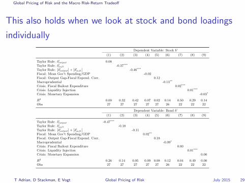
This also holds when we look at stock and bond loadings
individually
Table 7: Global Risk Loadings and Policy Tools
This table reports results from cross-sectional regressions of global risk loadings bi on the indicatedpolicy variables. The global risk loadings bi are obtained from sieve reduced rank regressions (SRRR)Et[Rxi
t+h] = ↵i + bi�h(vixt). The index i ranges over the global market excess return (MKT), 27country stock returns, and corresponding 27 10-year sovereign bond excess returns in the SRRRestimation. The resulting 27 bi country stock return loadings and 27 bi bond return loadings formthe dependent variables in the table below. The forecast horizon is h = 6 months, and the sampleconsists of an unbalanced panel of observations from 1990:1 to 2014:12. All returns are expressed inUS dollars.
Dependent Variable: Stock bi
(1) (2) (3) (4) (5) (6) (7) (8) (9)
Taylor Rule: �ioutput 0.08
Taylor Rule: �iinfl -0.37***
Taylor Rule:���i
output
�� +���i
infl
�� -0.46***
Fiscal: Mean Gov’t Spending/GDP -0.02Fiscal: Output Gap-Fiscal Expend. Corr. 0.12Macroprudential -0.13**
Crisis: Fiscal Bailout Expenditure 0.02***
Crisis: Liquidity Injection 0.01***
Crisis: Monetary Expansion -0.03*
R2 0.00 0.32 0.42 0.07 0.02 0.14 0.50 0.29 0.14Obs 27 27 27 27 27 26 22 22 22
Dependent Variable: Bond bi
(1) (2) (3) (4) (5) (6) (7) (8) (9)
Taylor Rule: �ioutput -0.47***
Taylor Rule: �iinfl -0.18
Taylor Rule:���i
output
�� +���i
infl
�� -0.11Fiscal: Mean Gov’t Spending/GDP 0.02**
Fiscal: Output Gap-Fiscal Expend. Corr. 0.18Macroprudential -0.09*
Crisis: Fiscal Bailout Expenditure 0.00Crisis: Liquidity Injection 0.01***
Crisis: Monetary Expansion 0.00
R2 0.26 0.14 0.05 0.09 0.08 0.12 0.04 0.49 0.00Obs 27 27 27 27 27 26 22 22 22
Dependent Variable: (Stock bi + Bond bi)
(1) (2) (3) (4) (5) (6) (7) (8) (9)
Taylor Rule: �ioutput -0.39*
Taylor Rule: �iinfl -0.54***
Taylor Rule:���i
output
�� +���i
infl
�� -0.57***
Fiscal: Mean Gov’t Spending/GDP -0.00Fiscal: Output Gap-Fiscal Expend. Corr. 0.30Macroprudential -0.22***
Crisis: Fiscal Bailout Expenditure 0.03***
Crisis: Liquidity Injection 0.02***
Crisis: Monetary Expansion -0.03
R2 0.06 0.44 0.40 0.00 0.07 0.25 0.37 0.53 0.07Obs 27 27 27 27 27 26 22 22 22
13
T Adrian, D Stackman, E Vogt Global Pricing of Risk July 2015 29

Global Pricing of Risk and the Macro Risk-Return Tradeoff
Takeaway from the Macro Risk-Return Tradeoff
1. Higher exposure to the global pricing of risk corresponds to higher
growth and higher volatility
I Macro risk-return tradeoff
2. Economic policies are systematically related to price of risk exposures
I Monetary policy
I Fiscal policy
I Macroprudential policy
How does pricing of risk interact with economic policies?
T Adrian, D Stackman, E Vogt Global Pricing of Risk July 2015 30
The Macro Risk-Return Tradeoff and Economic Policies
Outline
Global Institutions and Global Pricing of Risk
Global Pricing of Risk and the Macro Risk-Return Tradeoff
The Macro Risk-Return Tradeoff and Economic Policies
T Adrian, D Stackman, E Vogt Global Pricing of Risk July 2015 31
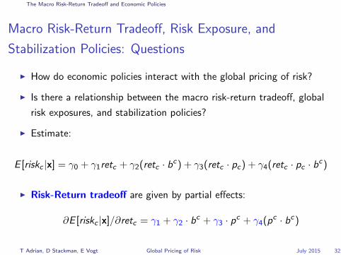
The Macro Risk-Return Tradeoff and Economic Policies
Macro Risk-Return Tradeoff, Risk Exposure, and
Stabilization Policies: Questions
I How do economic policies interact with the global pricing of risk?
I Is there a relationship between the macro risk-return tradeoff, global
risk exposures, and stabilization policies?
I Estimate:
E [riskc |x] = γ0 + γ1retc + γ2(retc · bc) + γ3(retc · pc) + γ4(retc · pc · bc)
I Risk-Return tradeoff are given by partial effects:
∂E [riskc |x]/∂retc = γ1 + γ2 · bc + γ3 · pc + γ4(pc · bc)
T Adrian, D Stackman, E Vogt Global Pricing of Risk July 2015 32

The Macro Risk-Return Tradeoff and Economic Policies
Macro Risk-Return Tradeoff
∂E [riskc |x]/∂retc = γ1 + γ2 · bc + γ3 · pc + γ4(pc · bc)
T Adrian, D Stackman, E Vogt Global Pricing of Risk July 2015 33

The Macro Risk-Return Tradeoff and Economic Policies
Macro Risk-Return Tradeoff and Monetary Policy
Table 8: Macro Risk-Return Tradeo↵s, Global Pricing of Risk, and Monetary PolicyStance
This table reports results from cross-sectional regressions of macro stability outcomes on globalrisk loadings, policies, macro control variables, and their interactions. The baseline regression isriski = �0 + �1ri + �2(ri · bi) + �3(ri · pi) + �4(ri · bi · pi) + "i, where riski denotes a macroeconomicor financial risk measure as indicated in the table headers, ri is the corresponding macroeconomic orfinancial return, and pi denotes country i’s policy stance as given by a measure of total Taylor rule
aggressiveness (pi =���output
i
�� +����infl
i
���). The global risk loadings bi are obtained from sieve reduced
rank regressions (SRRR) Et[Rxit+h] = ↵i + bi�h(vixt). The index i ranges over the global market
excess return (MKT), 27 country stock returns, and corresponding 27 10-year sovereign bond excessreturns in the SRRR estimation. The resulting 27 bi country stock return loadings and 27 bi bondreturn loadings are used as independent variables in the table below. The forecast horizon is h = 6months, and the sample consists of an unbalanced panel of observations from 1990:1 to 2014:12. Allreturns are expressed in US dollars.
GDP Volatility Inflation Volatility
(1) (2) (3) (4) (1) (2) (3) (4)
r 0.96*** �1.04** �0.13 �0.20 1.59*** 2.06*** 2.13*** 2.38***
r · b 1.02*** 0.57* 0.61* �0.91*** �0.97*** �1.56***
r · p �0.50** �0.41 �0.10 �0.47r · b · p �0.07 1.22*
R2 0.45 0.55 0.60 0.60 0.78 0.83 0.83 0.85Obs 27 27 27 27 27 27 27 27
Crisis Peak NPL Bank Flows Volatility
(1) (2) (3) (4) (1) (2) (3) (4)
r 8.01 �47.01*** �33.45* �106.26*** 0.93 0.58 2.16* 2.62**
r · b 38.61*** 31.86*** 81.72*** 1.39 0.25 �2.85r · p �7.10 89.59** �1.62** �2.26***
r · b · p �70.11** 3.98**
R2 0.12 0.38 0.39 0.44 0.09 0.11 0.26 0.32Obs 22 22 22 22 24 24 24 24
Equity Downside Volatility Yield Upside Volatility
(1) (2) (3) (4) (1) (2) (3) (4)
r 0.00 �5.22*** �5.15*** �4.35*** 0.14*** 0.19* 0.15* 0.16r · b 4.14*** 4.10*** 3.52*** �0.04 �0.04 �0.06r · p �0.04 �1.06 0.07** 0.06r · b · p 0.84 0.03
R2 0.00 0.68 0.68 0.68 0.29 0.30 0.40 0.40Obs 27 27 27 27 27 27 27 27
14
T Adrian, D Stackman, E Vogt Global Pricing of Risk July 2015 34

The Macro Risk-Return Tradeoff and Economic Policies
Macro Risk-Return Tradeoff and Fiscal Policy
Table 9: Macro Risk-Return Tradeo↵s, Global Pricing of Risk, and Fiscal Policy Stance
This table reports results from cross-sectional regressions of macro stability outcomes on globalrisk loadings, policies, macro control variables, and their interactions. The baseline regression isriski = �0 + �1ri + �2(ri · bi) + �3(ri · pi) + �4(ri · bi · pi) + "i, where riski denotes a macroeconomicor financial risk measure as indicated in the table headers, ri is the corresponding macroeconomic orfinancial return, and pi denotes country i’s policy stance as given by the degree of countercyclicalityof fiscal policies to output gap deviations. The global risk loadings bi are obtained from sieve reducedrank regressions (SRRR) Et[Rxi
t+h] = ↵i + bi�h(vixt). The index i ranges over the global marketexcess return (MKT), 27 country stock returns, and corresponding 27 10-year sovereign bond excessreturns in the SRRR estimation. The resulting 27 bi country stock return loadings and 27 bi bondreturn loadings are used as independent variables in the table below. The forecast horizon is h = 6months, and the sample consists of an unbalanced panel of observations from 1990:1 to 2014:12. Allreturns are expressed in US dollars.
GDP Volatility Inflation Volatility
(1) (2) (3) (4) (1) (2) (3) (4)
r 0.96*** �1.04** �0.50 �0.51 1.59*** 2.06*** 2.07*** 2.41***
r · b 1.02*** 0.82*** 0.83** �0.91*** �0.93** �1.18***
r · p �0.49** �0.44 �0.02 �1.09**
r · b · p �0.03 2.72**
R2 0.45 0.55 0.63 0.63 0.78 0.83 0.83 0.86Obs 27 27 27 27 27 27 27 27
Crisis Peak NPL Bank Flows Volatility
(1) (2) (3) (4) (1) (2) (3) (4)
r 8.01 �47.01*** �42.10*** �4.01 0.93 0.58 0.19 0.35r · b 38.61*** 37.56*** 12.97 1.39 1.49 0.94r · p �13.52* �133.42** 0.70 0.20r · b · p 76.53* 1.57
R2 0.12 0.38 0.43 0.45 0.09 0.11 0.13 0.13Obs 22 22 22 22 24 24 24 24
Equity Downside Volatility Yield Upside Volatility
(1) (2) (3) (4) (1) (2) (3) (4)
r 0.00 �5.22*** �5.24*** �5.05*** 0.14*** 0.19* 0.20* 0.22**
r · b 4.14*** 4.14*** 3.98*** �0.04 �0.06 �0.08r · p 0.15 �0.81 �0.02 �0.09r · b · p 0.70 0.19
R2 0.00 0.68 0.68 0.68 0.29 0.30 0.30 0.33Obs 27 27 27 27 27 27 27 27
15
T Adrian, D Stackman, E Vogt Global Pricing of Risk July 2015 35

The Macro Risk-Return Tradeoff and Economic Policies
Macro Risk-Return Tradeoff and Macroprudential Policy
Table 10: Macro Risk-Return Tradeo↵s, Global Pricing of Risk, and MacroprudentialPolicy Stance
This table reports results from cross-sectional regressions of macro stability outcomes on globalrisk loadings, policies, macro control variables, and their interactions. The baseline regression isriski = �0 + �1ri + �2(ri · bi) + �3(ri · pi) + �4(ri · bi · pi) + "i, where riski denotes a macroeconomicor financial risk measure as indicated in the table headers, ri is the corresponding macroeconomic orfinancial return, and pi denotes country i’s policy stance as given by the degree of countercyclicalityof fiscal policies to output gap deviations. The global risk loadings bi are obtained from sieve reducedrank regressions (SRRR) Et[Rxi
t+h] = ↵i + bi�h(vixt). The index i ranges over the global marketexcess return (MKT), 27 country stock returns, and corresponding 27 10-year sovereign bond excessreturns in the SRRR estimation. The resulting 27 bi country stock return loadings and 27 bi bondreturn loadings are used as independent variables in the table below. The forecast horizon is h = 6months, and the sample consists of an unbalanced panel of observations from 1990:1 to 2014:12. Allreturns are expressed in US dollars.
GDP Volatility Inflation Volatility
(1) (2) (3) (4) (1) (2) (3) (4)
r 0.99*** �0.99** �0.13 �1.07 1.59*** 2.06*** 2.54*** 2.65***
r · b 1.00*** 0.67** 1.48*** �0.91*** �1.32*** �1.89***
r · p �0.88** 2.11* �1.17** �1.55***
r · b · p �2.61** 2.61***
R2 0.46 0.56 0.65 0.72 0.78 0.83 0.88 0.90Obs 26 26 26 26 26 26 26 26
Crisis Peak NPL Bank Flows Volatility
(1) (2) (3) (4) (1) (2) (3) (4)
r 7.38 �47.64*** �53.77*** �36.88*** 0.93 0.57 1.40 1.70r · b 38.61*** 41.80*** 28.92*** 1.39 0.19 �1.36r · p 7.12 �84.99 �2.05** �2.53**
r · b · p 74.91* 3.29
R2 0.10 0.37 0.38 0.42 0.09 0.11 0.22 0.23Obs 21 21 21 21 23 23 23 23
Equity Downside Volatility Yield Upside Volatility
(1) (2) (3) (4) (1) (2) (3) (4)
r 0.09 �5.26*** �5.34*** �4.93*** 0.15*** 0.20** 0.21** 0.22*
r · b 4.16*** 4.20*** 3.82*** �0.05 �0.06 �0.08r · p 0.15 �1.51 �0.02 �0.03r · b · p 1.55 0.06
R2 0.00 0.67 0.67 0.67 0.31 0.32 0.33 0.33Obs 26 26 26 26 26 26 26 26
16
T Adrian, D Stackman, E Vogt Global Pricing of Risk July 2015 36
Conclusion
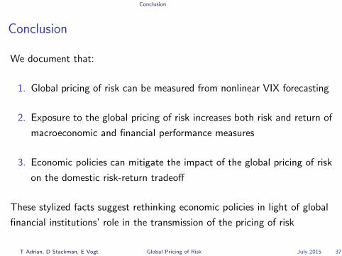
Conclusion
We document that:
1. Global pricing of risk can be measured from nonlinear VIX forecasting
2. Exposure to the global pricing of risk increases both risk and return of
macroeconomic and financial performance measures
3. Economic policies can mitigate the impact of the global pricing of risk
on the domestic risk-return tradeoff
These stylized facts suggest rethinking economic policies in light of global
financial institutions’ role in the transmission of the pricing of risk
T Adrian, D Stackman, E Vogt Global Pricing of Risk July 2015 37

Conclusion
To do list
1. Instrumenting for the policies
2. Dynamic interactions
3. Magnitudes
T Adrian, D Stackman, E Vogt Global Pricing of Risk July 2015 38

Literature
Adrian, T., and N. Boyarchenko (2012): “Intermediary Leverage Cyclesand Financial Stability,” Federal Reserve Bank of New York Staff Report, 567.
Adrian, T., R. Crump, and E. Vogt (2015): “Nonlinearity and flight tosafety in the risk-return trade-off for stocks and bonds,” Federal Reserve Bankof New York Staff Report, 723.
Adrian, T., and H. S. Shin (2014): “Procyclical Leverage and Value atRisk,” Review of Financial Studies, 27(2), 373–403.
Bekaert, G., M. Hoerova, and M. L. Duca (2013): “Risk, uncertaintyand monetary policy,” Journal of Monetary Economics, 60(7), 771–788.
Borio, C., and H. Zhu (2012): “Capital regulation, risk-taking and monetarypolicy: a missing link in the transmission mechanism?,” Journal of FinancialStability, 8(4), 236–251.
He, Z., and A. Krishnamurthy (2008): “Intermediary asset pricing,”Discussion paper, National Bureau of Economic Research.
(2011): “A model of capital and crises,” The Review of EconomicStudies, p. rdr036.
T Adrian, D Stackman, E Vogt Global Pricing of Risk July 2015 39

Literature
Longstaff, F. A., J. Pan, L. H. Pedersen, and K. J. Singleton(2011): “How Sovereign Is Sovereign Credit Risk?,” American EconomicJournal: Macroeconomics, 3(2), 75–103.
Miranda-Agrippino, S., and H. Rey (2014): “World Asset Markets and theGlobal Financial Cycle,” Discussion paper, Technical Report, Working Paper,London Business School.
Panageas, S., and M. M. Westerfield (2009): “High-Water Marks: HighRisk Appetites? Convex Compensation, Long Horizons, and Portfolio Choice,”The Journal of Finance, 64(1), 1–36.
Rey, H. (2015): “Dilemma not trilemma: the global financial cycle andmonetary policy independence,” Discussion paper, National Bureau ofEconomic Research.
Vayanos, D. (2004): “Flight to quality, flight to liquidity, and the pricing ofrisk,” Discussion paper, National Bureau of Economic Research.
T Adrian, D Stackman, E Vogt Global Pricing of Risk July 2015 40