Stability of Feature Selection Algorithms:a study on high dimensional spaces

Alexandros Kalousis, Julien Prados, Melanie HilarioUniversity of Geneva, Computer Science DepartmentRue General Dufour 24, 1211 Geneva 4, Switzerland

{kalousis, prados, hilario}@cui.unige.ch

Abstract

With the proliferation of extremely high-dimensional data, feature selection algorithms have become indispensable com-ponents of the learning process. Strangely, despite extensive work on the stability of learning algorithms, the stability offeature selection algorithms has been relatively neglected. This study is an attempt to fill that gap by quantifying the sensi-tivity of feature selection algorithms to variations in thetraining set. We assess the stability of feature selection algorithmsbased on the stability of the feature preferences that they express in the form of weights-scores, ranks, or a selected featuresubset. We examine a number of measures to quantify the stability of feature preferences and propose an empirical way toestimate them. We perform a series of experiments with several feature selection algorithms on a set of proteomics datasets.The experiments allow us to explore the merits of each stability measure and create stability profiles of the feature selectionalgorithms. Finally we show how stability profiles can support the choice of a feature selection algorithm.

1 Introduction

High dimensional datasets are becoming more and more abundant in classification problems. A variety of feature selectionmethods have been developed to tackle the issue of high dimensionality. The major challenge in these applications is to extracta set of features, as small as possible, that accurately classifies the learning examples.

A relatively neglected issue in the work on high dimensionalproblems, and in general in problems requiring featureselection, is the stability of the feature selection methods used. Stability, defined as the sensitivity of a method to variationsin the training set, has been extensively studied with respect to the learning algorithm itself. We propose to investigate howdifferent subsamples of a training set affect a method’s assessment of a feature’s importance and consequently the finalset ofselected features.

The stability of classification algorithms was examined by Turney [16] who proposed a measure based on the agreementof classification models produced by an algorithm when trained on different training sets. He defined the agreement of twoclassification models as the probability that they will produce the same predictions over all possible instances drawn froma probability distributionP (X). Note that instances are drawn fromP (X) and not fromP (X, C), the joint probabilitydistribution of class and training instances; the underlying reason is that the agreement of two concepts—classificationmodels—should be examined in all possible input worlds. In order to estimate stability he suggested usingm× 2-fold cross-validation. In each of them repetitions of cross-validation a classification model is produced from each one of the two folds.The two models are then tested on artificial instances drawn by sampling fromP (X) and their agreement is computed. Thefinal estimation of stability is the average agreement over all m runs.

Related to the notion of stability is the bias-variance decomposition of the error of classification algorithms, [6, 2, 3]. Thevariance term quantifies instability of the classification algorithm in terms of classification predictions. Variance measuresthe percentage of times that the predictions of different classification models, learned from different training sets,for a giveninstance are different from the typical (average) prediction. Bias-variance decomposition is usually done via bootstrapping,where part of the data is kept as a hold-out test set and the remainder is used to create different training sets by using samplingwith replacement. The final estimation of variance is also the average over the different bootstrap samples.

In both approaches described above, the predictions of the classification models are crucial in quantifying the sensitivityof classification algorithms to changes in the training sets(note that both approaches can also be used for error estimationwhich is then tightly coupled with the stability analysis).However when one wants to examine only feature selection algo-rithms without involving a classification algorithm, the above methods do not apply. Typical feature selection algorithms donot construct classification models and thus cannot provideclassification predictions. They usually output what we call afeature preference statement (for conciseness,feature preference); this can take the form of a subset of selected features, oralternatively of a weighting-scoring or a ranking of the features, based on which a small set of features can be selected (eitherby specifying a threshold or asking for a specific number of features). A classification algorithm should then be applied onthe selected feature set to produce a classification model. If we used the stability estimation methods described above tothe combined feature selection and classification algorithms, we would be measuring their joint sensitivity to training setvariations and we would have no way to delimit the (in)stability the feature selection algorithm from that of the classificationalgorithm.

To address this difficulty we introduce the notion of preferential stability, i.e., the stability of the feature preferencesproduced by a feature selection algorithm, to quantify its sensitivity to differences in training sets drawn from the samedistribution. The same approach can in fact be used to measure the preferential stability of any classification algorithm thatproduces models from which weightings or rankings of the features can be extracted, e.g. linear discrimination algorithms.

Stability, as introduced in [16], and the bias-variance decomposition frameworks are not able to accurately quantify pref-erential stability. It is possible that different trainingsamples lead to really different feature sets which howeveryield thesame prediction patterns. This can be especially true when the initial features have a high level of redundancy which is nothandled in a principled way by the algorithms used.

The motivation for investigating the stability of feature selection algorithms came from the need to provide applicationdomain experts with quantified evidence that the selected features are relatively robust to variations in the training data. Thisneed is particularly crucial in biological applications, e.g. genomics, DNA-micorarrays, and proteomics, mass spectrometry.These applications are typically characterized by high dimensionality, the goal is to output a small set of highly discriminatoryfeatures on which biomedical experts will subsequently invest considerable time and research effort. Domain experts tendto have less confidence in feature sets that change radicallywith slight variations in the training data. Data miners have toconvince them not only of the predictive potential but also of the relative stability of the proposed features.

The rest of the paper is organized as follows: in Section 2 we introduce measures of stability that can be applied to anyfeature selection algorithm that outputs a feature preference as defined above; we also show how we can empirically estimatethese measures. In Section 3 we describe the experimental setup, the datasets used, and the feature selection algorithmsincluded in the study; in Section 4 we present the results of the experiments, investigate the behavior of the different stabilitymeasures and establish the stability profiles of the chosen feature selection algorithms; in Section 5 we examine togetherclassification performance and stability of feature preferences, and suggest how we can exploit the latter to support thechoice of the appropriate feature selection algorithm; finally we conclude in Section 6.

2 Stability

The generic model of classification comprises: a generator of random vectorsx, drawn according to an unknown but fixedprobability distributionP (X); a supervisor that assigns class labelsc, to thex random vectors, according to an unknown butfixed conditional probability distributionP (C|X); a learning space populated by pairs(x, c) drawn from the joint probabilitydistributionP (X, C) = P (C|X)P (X).

We define thestabilityof a feature selection algorithm as the robustness of the feature preferences it produces to differencesin training sets drawn from the same generating distribution P (X, C). Stability quantifies how different training sets affectthe feature preferences.

Measuring stability requires a similarity measure for feature preferences. This obviously depends on the representationlanguage used by a given feature selection algorithm to describe its feature preferences; different representation languagescall for different similarity measures. We can distinguishthree types of representation languages for feature preferences. Inthe first type a weight or score is assigned to each feature indicating its importance. The second type of representation is asimplification of the first where instead of weights ranks areassigned to features. The third type consists of sets of selectedfeatures in which no weighting or ranking is considered. Obviously any weighting schema can be cast as a ranking schema,which in turn can be cast as a set of features by setting a threshold on the ranks or asking for a given number of features.

More formally, let training examples be described by a vector of featuresf = (f1, f2, ..., fm), then a feature selectionalgorithm produces either:

• a weighting-scoring:w = (w1, w2, .., wm), w ∈ W ⊆ Rm,

• a ranking:r = (r1, r2, .., rm), 1 ≤ ri ≤ m,

• or a subset of features:s = (s1, s2, .., sm), si ∈ {0, 1}, with 0 indicating absence of a feature and1 presence.

In order to measure stability we need a measure of similarityfor each of the above representations. To measure similaritybetween two weightingsw, w′, produced by a given feature selection algorithm we use Pearson’s correlation coefficient

SW (w, w′) =

∑

i(wi − µw)(w′

i− µw′)

√∑

i(wi − µw)2

∑

i(w′

i− µw′)2

,

whereSW takes values in [-1,1]; a value of 1 means that the weightingsare perfectly correlated, a value of 0 that there is nocorrelation while a value of -1 that they are anticorrelated.

To measure similarity between two rankingsr, r′, we use Spearman’s rank correlation coefficient

SR(r, r′) = 1 − 6∑

i

(ri − r′i)2

m(m2 − 1),

whereri andr′i

are the ranks of featurei in rankingsr andr′ respectively. Here too the possible range of values is in [-1,1].A value of 1 means that the two rankings are identical, a valueof 0 that there is no correlation between the two ranks, and avalue of -1 that they have exactly inverse orders.

Finally we measure similarity between two subsets of features using a straightforward adaptation of the Tanimoto distancebetween two sets, [4]:

SS(s, s′) = 1 −|s| + |s′| − 2|s ∩ s′|

|s| + |s′| − |s ∩ s′|.

The Tanimoto distance metric measures the amount of overlapbetween two sets of arbitrary cardinality.SS takes values in[0,1] with 0 meaning that there is no overlap between the two sets, and 1 that the two sets are identical.

To empirically estimate the stability of a feature selection algorithm for a given dataset, we can simulate the distributionP (X, C) from which the training sets are drawn by using a resampling technique like bootstrapping or cross-validation. Weopted for N-fold stratified cross-validation (N=10). In ten-fold cross-validation the overlap of training instances among thedifferent training folds is roughly 78%. The feature selection algorithm outputs a feature preference for each of the trainingfolds. The similarity of each pair of feature preferences, i.e.N(N − 1)/2 pairs, is computed using the appropriate similaritymeasure and the final stability score is simply the average similarity over all pairs.

We want to couple stability estimates with classification error estimates in view of identifying feature selection algorithmswhich maximize both stability and classification performance. To this end we embed the procedure described above withinanerror estimation procedure, itself conducted using stratified 10-fold cross-validation. In other words, at each iteration of thecross-validated error estimation loop, there is a full internal cross-validation loop aimed at measuring the stability of featureprecedences returned by the feature selection algorithm. The outer loop provides a classification error estimate in theusualmanner, while the inner loop provides an estimate of the stability of the feature selection algorithm.

3 Stability Experiments

3.1 Datasets

We have chosen to experiment with high dimensional data fromthree different application domains, namely proteomics,genomics and text mining. A short description of these datasets is given in table 1.

The proteomics datasets come all from the domain of mass-spectrometry. The goal is to construct classification modelsthat discriminate between healthy and diseased individuals, i.e we have two class problems. We worked with three differentdatasets:ovarian cancer [11], (version 8-07-02),prostate cancer [12] and an extended version of the earlystroke diagnosisdataset used in [14]. All features correspond to intensities of mass values and are continuous.

The genomics datasets are all datasets of DNA-microarray experiments. We worked with three different datasets:leukemia[7] where the goal is to distinguish between acute myeloid leukemia (AML) and acute lymphoblastic leukemia (ALL); clas-sification of embryonal tumors of the centralnervous system [13] where the goal is to predict whether a given treatment

dataset class 1 # class 1 class 2 # class 2 # featuresovarian normal 91 diseased 162 824prostate normal 253 diseased 69 2200stroke normal 101 diseased 107 4928leukemia ALL 47 AML 25 7131nervous survival 21 failure 39 7131colon normal 22 tumor 40 2000alt relevant 1425 not 2732 2112disease relevant 631 not 2606 2376function relevant 818 not 3089 2708structure relevant 927 not 2621 2368subcell relevant 1502 not 6475 4031

Table 1. Description of datasets.

will be effective or not (i.e., patient will or will not survive); andcolon cancer [1] where the goal is to distinguish betweenhealthy and tumor colon tissue. Features correspond to levels of expression of different genes and are continuous.

In text mining we worked with five datasets aimed at determining whether a sentence is relevant or not to a given topic:protein-disease relations (disease), protein-function and structure (function andstructure respectively), protein subcellularlocation (subcell), and related protein sequences produced by alternative splicing of a gene or by the use of alternativeinitiation codons (alt) [10]. Sentence features are stemmed words, each describedby a continuous value representing itstandardtf-idf score.

Dimensionality reduction and stability of selected features are very important especially in the first two types of applica-tions. The selected features provide the basis to distinguish between different types of pathologies, a first path to hypothesisconstruction, an initial understanding of the mechanisms involved in various diseases etc. In other words they provideastarting point which is followed by substantial laboratoryresearch. As such the quality and the robustness of the selectedfeatures is of paramount importance.

3.2 Feature Selection Algorithms

For feature selection we considered the following methods:Information Gain (IG), Chi-Square (CHI) [4], SymmetricalUncertainty (SYM), [9], ReliefF (RELIEF), [15], and SVMRFE[8]. Information gain, Chi-Square and Symmetrical Uncer-tainty are all univariate feature scoring methods for nominal attributes or continuous attributes which are discretized using themethod of [5]. ReliefF delivers a weighting of the features while taking their interactions into account; it uses all features tocompute distances among training instances and the K nearest neighbors of each of theM probe instances to update featureweights. We setK to 10 andM to the size of the training set, so that all instances were used as probes. SVMRFE is basedon repetitive applications of a linear support vector machine algorithm where theP% lowest ranked features are eliminatedat each iteration of the linear SVM. The ranks of the featuresare based on the absolute values of the coefficients assignedtothem by the linear SVM. In our experiments,P was set to 10% and the complexity parameterC of the linear SVM to 0.5.

We also include a simple linear support vector machine to show that the same type of stability analysis can be appliedto any linear classifier; here too the complexity parameter was set to 0.5. Provided that all features are normalized to acommon scale, the absolute values or the squares of the coefficients of the linear hyperplane can be taken to reflect theimportance of the corresponding features, in effect providing a feature weighting. This is actually the assumption underwhich SVMRFE works; alternatively the support vector machine is equivalent to SVMRFE with a single iteration, where theranking of the features is simply based on the absolute values or the squares of the coefficients of the support vector machine.We consider this version of support vector machines as yet another feature selection algorithm and identify it as SVMONE.The implementations of all the algorithms are those found inthe WEKA machine learning environment [17].

As already mentioned the stability estimates are calculated within each training fold by a nested cross-validation loop andthe final results reported are the averages,SW , SR, SS , over the ten external folds.

dataset IG CHI SYMSW SR SS SW SR SS SW SR SS

ovarian 0.9553 0.9105 0.4948 0.9560 0.9089 0.5614 0.9512 0.9068 0.5038prostate 0.8247 0.4070 0.4080 0.8249 0.4011 0.4212 0.8196 0.4039 0.4125stroke 0.8387 0.2042 0.1847 0.8434 0.2032 0.2152 0.8250 0.2023 0.2187avg 0.8729 0.5072 0.3625 0.8747 0.5044 0.3992 0.8652 0.5043 0.3783

leukemia 0.8507 0.2492 0.7392 0.8467 0.2477 0.7557 0.8397 0.2479 0.7897nervous 0.4652 0.0177 0.2320 0.4693 0.0166 0.2385 0.4652 0.0182 0.2436colon 0.7606 0.1138 0.4865 0.7587 0.1157 0.5024 0.7504 0.1159 0.5069average 0.6921 0.1269 0.4859 0.6915 0.1266 0.4988 0.6851 0.1273 0.5134

alt 0.9983 0.1254 0.9632 0.9985 0.1267 0.9640 0.9966 0.1268 0.9037disease 0.9231 0.0900 0.7589 0.9267 0.0853 0.7470 0.9002 0.0853 0.7405function 0.9151 0.1045 0.8055 0.9255 0.1058 0.7974 0.8972 0.1041 0.7491structure 0.9771 0.1636 0.8855 0.9807 0.1641 0.8853 0.9643 0.1629 0.8485subcell 0.9854 0.1136 0.8990 0.9873 0.1139 0.8599 0.9795 0.1135 0.8487average 0.9594 0.1194 0.8624 0.9637 0.1191 0.8507 0.9476 0.1185 0.8181

average

RELIEF SVMONE SMVRFESW SR SS SW SR SS SW SR SS

ovarian 0.9697 0.9537 0.7296 0.9379 0.8476 0.5965 NA 0.8386 0.4680prostate 0.9572 0.9399 0.5529 0.8685 0.7389 0.5243 NA 0.7323 0.4484stroke 0.8806 0.8230 0.3410 0.8174 0.7032 0.2721 NA 0.6971 0.1678avg 0.9358 0.9055 0.5411 0.8746 0.7633 0.4175 NA 0.7560 0.3614

leukemia 0.9157 0.8675 0.5793 0.8757 0.7655 0.4878 NA 0.7632 0.2678nervous 0.8078 0.7839 0.2873 0.8099 0.6751 0.4568 NA 0.6728 0.1065colon 0.9063 0.8363 0.6931 0.7782 0.6818 0.3512 NA 0.6799 0.2392average 0.8766 0.8292 0.5199 0.8213 0.7074 0.4319 NA 0.7053 0.2045

alt 0.8278 0.6945 0.6908 0.9889 0.7468 0.6676 NA 0.7307 0.6517disease 0.8270 0.6892 0.5277 0.8366 0.7033 0.5269 - - -function 0.6764 0.6417 0.5444 0.7826 0.7169 0.3255 - - -structure 0.7636 0.6678 0.5072 0.8543 0.7156 0.5325 - - -subcell 0.8016 0.6881 0.6794 0.9328 0.7345 0.7663 - - -average 0.7793 0.6763 0.5899 0.8790 0.7234 0.5638

Table 2. Stability results for the different stability meas ures. SS is computed on feature sets com-prising the top ten features proposed by each method.

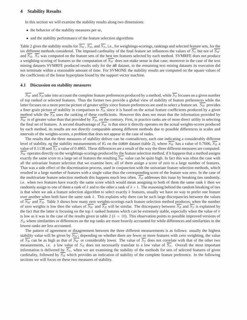
4 Stability Results

In this section we will examine the stability results along two dimensions:

• the behavior of the stability measures per se,

• and the stability performance of the feature selection algorithms

Table 2 gives the stability results forSW , SR, andSS , i.e., for weightings-scorings, rankings and selected feature sets, for thesix different methods considered. The imposed cardinalityof the final feature set influences the values ofSS but not ofSW

andSR. SS was computed on the feature sets of the best ten features selected by each method. SVMRFE does not producea weighting-scoring of features so the computation ofSW does not make sense in that case; moreover in the case of the textmining datasets SVMRFE produced results only for thealt dataset, in the remaining text mining datasets its execution didnot terminate within a reasonable amount of time. For SVMONEthe stability results are computed on the square values ofthe coefficients of the linear hyperplane found by the support vector machine.

4.1 Discussion on stability measures

SW andSR take into account the complete feature preferences produced by a method, whileSS focuses on a given numberof top ranked or selected features. Thus the former two provide a global view of stability of feature preferences while thelatter focuses on a more precise picture of greater utility since feature preferences are used to select a feature set.SW providesa finer grain picture of stability in comparison toSR since it is based on the actual feature coefficients producedby a givenmethod while theSR uses the ranking of these coefficients. However this does notmean that the information provided bySW is of greater value than that provided bySR, on the contrary. First, in practice ranks are of more directutility in selectingthe final set of features. A second disadvantage ofSW is that since it directly operates on the actual weights-scores producedby each method, its results are not directly comparable among different methods due to possible differences in scales andintervals of the weights-scores, a problem that does not appear in the case of ranks.

The results that the three measures of stability deliver canbe contradictory, each one indicating a considerably differentlevel of stability, eg the stability measurements of IG on the colon dataset (table 2), whereSW has a value of 0.7606,SR avalue of 0.1138 andSS a value of 0.4865. These differences are a result of the way the three different measures are computed.SW operates directly on the weightings-scorings produced by the feature selection method, if it happens that a method assignsexactly the same score to a large set of features the resulting SW value can be quite high. In fact this was often the case withall the univariate feature selection that we examine here, all of them assign a score of zero to a large number of features.That was a side effect of the discretization process, used inconjunction with the univariate feature selection methods, whichresulted in a large number of features with a single value thus the corresponding score of the feature was zero. In the caseofthe multivariate feature selection methods this happens much less often.SR addresses this issue by breaking ties randomly,i.e. when two features have exactly the same score which would mean assigning to both of them the same rankk then werandomly assign to one of them a rank ofk and to the other a rank ofk+1. The reasoning behind the random breaking of tiesis that when we ask a feature selection algorithm to select exactly k features, usually we have no way to prefer one featureover another when both have the same rankk. This explains why there can be such large discrepancies between the valuesof SW andSR. Table 3 shows how many zero weights-scorings each feature selection method produces; when the numberof zero weights is low then the values ofSW andSR will be similar. The discrepancy betweenSR andSS is explained bythe fact that the latter is focusing on the topk ranked features which can be extremely stable, especially when the value ofkis low as it was in the case of the results given in table 2 (k = 10). This observation points to possible improved versions ofSR where similarities or differences on the top ranks are more heavily accounted for while differences and similarities inthelowest ranks are less accounted.

The pattern of agreement or disagreement between the three different measurements is as follows: usually the higheststability value will be given bySW ; depending on whether there are fewer or more features with zero weighting, the valueof SR can be as high as that ofSW or considerably lower. The value ofSS does not correlate with that of the other twomeasurements, i.e. a low value ofSR does not necessarily translate to a low value ofSS . Overall the most importantinformation is delivered bySS , when we are examining the stability of the methods for sets of selected features of givencardinality, followed bySR which provides an indication of stability of the complete feature preference. In the followingsections we will focus on these two measures of stability.

IG CHI SYM RELIEF SVMONEovarian 35.07 35.07 35.07 0 01.08prostate 85.63 85.63 85.63 0 00.99stroke 91.25 91.25 91.25 0 02.33leukemia 87.68 87.68 87.68 0 16.21nervous 98.48 98.48 98.48 0 09.91colon 93.98 93.98 93.98 0 02.51alt 94.33 94.33 94.33 05.56 09.72disease 96.15 96.15 96.15 06.06 05.03function 95.17 95.17 95.17 07.35 05.64structure 92.82 92.82 92.82 06.88 05.69subcell 95.19 95.19 95.19 06.13 07.91

Table 3. Percentage of features with zero score for each meth od.

4.2 Discussion on stability of feature selection algorithms

First of all there is no feature selection method that is consistently more stable than all the others for all the differentproblems that we examined. However it seems that there are types of problems for which a given method is more stable thanthe others.

In the case of the proteomics problems the most stable methodseems to be RELIEF which achieved the highest stabilityscores in all three problems both in terms ofSR andSS . The feature preferences that RELIEF produces for the giventype ofproblem are stable both globally, i.e. the ranking of the features does not change considerably with different trainingsets, andat the top, i.e. the ten top ranked features do not change considerably with changes in the training set. The global stability ofRELIEF’s feature preferences as measured bySR is on average 0.9055 for the three proteomics datasets, considerably higherthan all the other feature selection methods. ForSS RELIEF scores 0.7295, 0.5529 and 0.3410 for theovarian, prostateandstroke datasets respectively. These scores correspond to an average overlap of 8.43, 7.12 and 5.08 features, out of theten contained in the final set of selected features, among thedifferent subsets of the training folds1. The rest of the methodshave a considerably lower score.

In the case of the genomics datasets the picture is mixed. In terms of the global stability of the feature preferencesmeasured bySR the clear winner is again RELIEF, with an average score of 0.8292. The results of all the univariate methodsare catastrophic, on average around 0.126, a fact that is dueto the very large number of features to which these methodsassigned a score of zero resulting in random rankings for these features. SVMONE and SVMRFE have relatively stablefeature preferences, around 0.7. However when we turn toSS the picture changes. For theleukemia dataset the univariatemethods achieve the highest stability compared to all the other methods, the best being SYM with a score of 0.7897 (8.82common features out of ten on average); for thenervous dataset the most stable algorithm is by far SVMONE and forcolonRELIEF.

For the text mining problems in terms of the global stabilitythe clear winner is SVMONE, with anSR that is consistentlyhigher than 0.7 for all datasets, followed by RELIEF. All univariate methods have a very lowSR score, in the best case around0.16, again this is due to the large number of features to which these methods assign a score of zero. The picture changesradically when we examine the stability behavior with respect to SS . This time the most stable methods are the univariatemethods with an averageSS score always above 0.8 (8.88 common features).

Overall RELIEF produces very stable feature preferences asthese are evaluated bySR, being the most stable in all theproteomics and genomics datasets and the second most stablein the text mining datasets. When we evaluate the stability ofthe top ten selected features RELIEF is the clear winner in the proteomics datasets and on average the best for the genomicsdatasets. The univariate feature selection methods perform badly in terms of their global stability but better when we evaluatethe stability of the top ten features, in fact for the text mining applications they are by far more stable than the other methods.The SVM based algorithms are somewhere in the middle gettingthe second place in terms of global stability in two out ofthe three application domains (proteomics, genomics). In what concerns the stability of the top ten selected features they donot have an application domain in which they excel.

1It is easy to compute the actual number of common features when we know theSS score and the cardinality of the final feature set simply by thedefinition ofSS .

Examining the stability profiles of the different feature selection algorithms three groups of algorithms arise naturally,where the algorithms that belong to a given group share a verysimilar stability behavior. The first group consists of all theunivariate feature selection algorithms, the second contains SVMONE and SVMRFE, while RELIEF is a group on each ownsince it does not have a stability behavior similar to any of the other methods.

IG, SYM and CHI have almost identical stability scores for all three measures of stability and all application domainsconsidered. This is not a surprise since all of them are basedin a similar principle, i.e. they select individual features on thebasis of how well they discriminate among the different classes.

SVMONE and SVMRFE are quite similar in terms ofSR—a fact that can be easily explained since the ranking of featuresprovided by SVMONE can be considered as a less refined versionof the ranking provided by SVMRFE, the former being theresult of a single execution of the SVM algorithm and the latter the result of an iterative execution where each time 10% ofthelower ranked features are removed. However in terms ofSS SVMONE appears to be more stable; for the proteomics datasetsSVMONE has an average overlap of 7.47, 6.87, 4.27 features out of ten against 6.37, 6.19, 2.87 for SVMRFE forovarian,prostate andstroke respectively. In the case of genomics datasets the difference is even greater, SVMONE has an averagefeature overlap of 6.55, 6.27, 5.19 against 4.22, 1.92, 3.86for SVMRFE for leukemia, nervous andcolon respectively;finally in alt the only text dataset in which SVMRFE terminated, the difference is small: 8 and 7.9. Here too the fact thatSVMRFE is based on multiple iterations explains its higher instability on the top ten ranked features. When the differencesof the coefficients of two features are rather small and a choice is about to be made on which of the two to eliminate, differenttraining sets could result in opposite rankings for these two features thus eliminating a different feature each time.

The results of the estimation process ofSS can be very eloquently visualized, not only providing insight on the stabilityof each method, but also clearly indicating which features are considered important by each method. An example of such avisualization for one dataset from each application domainis given in figure 1, where the cardinality of the final featuresetis set to ten. In each of the graphs the x-axis corresponds to the individual features. The y-axis is separated into 10 rows,each one corresponding to one of the outer cross-validationfolds. Within each row we find 10 rows (not visibly separated)corresponding to each of the inner cross-validation folds of the outer fold. A perfectly stable method, i.e. one that alwayschooses the same features, would have in its graph as many vertical lines as the cardinality of the final feature set. Each linewould correspond to one selected feature.

Examining figure 1 it is obvious that the most stable behaviorfor all algorithms is attained for thealt dataset while theless stable in the case of thenervous dataset, withprostate being somewhere in the middle. In the case of thealt datasetit is clear that the univariate methods are more stable than RELIEF, SVMONE and SVMRFE. The visual inspection of thegraphs allows for a clear understanding of which features are considered most important by each method. We can see that thethree univariate methods select roughly the same features on each dataset. The feature patterns established by SVMONE andSVMRFE are also similar between them, albeit to a lesser extent, while RELIEF has a distinctively different pattern fromall the other methods. Moreover it is clear that the actual value of stability is affected by the dataset examined with somedatasets resulting in systematically higher levels of stability for all algorithms.

4.3 Stability profiles with SS

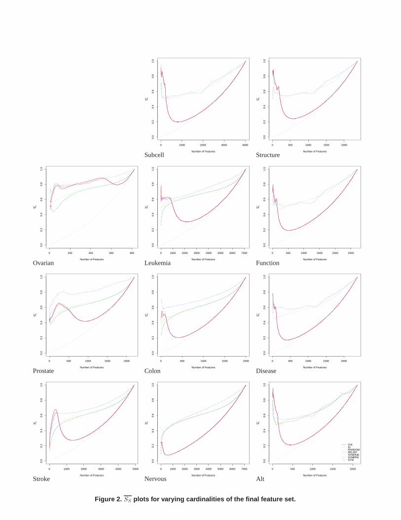
The more interesting stability estimation is provided bySS since it focuses on a subset of features, the ones selected byeach method, which is actually what interests us when we are performing feature selection. Nevertheless this estimation isspecific to a given number of selected features. To get a more global picture of the stability profile of the different methodswith respect toSS we computed its values for different sizes of selected feature sets, ranging from 10 up to the cardinality ofthe full feature set in increments of five, the results are given in figure 2. However as the cardinality of the selected featureset increases so does the estimated value of stability simply because with a larger number of selected features there is alsoa higher probability that there will be more features in common only due to chance. To quantify the increase in stabilityattributed to the increasing cardinality of the selected feature set we included as a stability baseline a random feature selectorthat outputs random feature sets of a given cardinality. We should note here that the computation of the curves does not requireany extra application of the feature selection algorithms other than that described in the previous section for estimating thedifferent stability measures, the reason is that each algorithm simply outputs a complete feature preference which canbereadily used to compute the values ofSS for different feature set cardinalities.

The univariate feature selection methods have an acceptable stability performance only for low cardinalities of feature setsfor almost all datasets, with the exception ofovarian. After a point their behavior converges to that of the randomselectorand they are dominated by the remaining three algorithms, a fact that as already mentioned is due to the discretization methodused with them. For low feature set cardinalities they dominate all other algorithms in all the text mining problems and they

500 1000 1500 2000

020

4060

8010

0

IG

Attribute Index

fold

s

500 1000 1500 2000

020

4060

8010

0

CHI

Attribute Index

fold

s

500 1000 1500 2000

020

4060

8010

0

SYM

Attribute Index

fold

s

500 1000 1500 2000

020

4060

8010

0

RELIEF

Attribute Index

fold

s

500 1000 1500 2000

020

4060

8010

0

SVMRFE

Attribute Index

fold

s

500 1000 1500 2000

020

4060

8010

0

SVMONE

Attribute Index

fold

s

Alt

1000 2000 3000 4000 5000 6000 7000

020

4060

8010

0

IG

Attribute Index

fold

s

1000 2000 3000 4000 5000 6000 7000

020

4060

8010

0

CHI

Attribute Index

fold

s

1000 2000 3000 4000 5000 6000 7000

020

4060

8010

0

SYM

Attribute Indexfo

lds

1000 2000 3000 4000 5000 6000 7000

020

4060

8010

0

RELIEF

Attribute Index

fold

s

1000 2000 3000 4000 5000 6000 7000

020

4060

8010

0

SVMRFE

Attribute Index

fold

s

1000 2000 3000 4000 5000 6000 7000

020

4060

8010

0SVMONE

Attribute Index

fold

sNervous

500 1000 1500 2000

020

4060

8010

0

IG

Attribute Index

fold

s

500 1000 1500 2000

020

4060

8010

0

CHI

Attribute Index

fold

s

500 1000 1500 2000

020

4060

8010

0

SYM

Attribute Index

fold

s

500 1000 1500 2000

020

4060

8010

0

RELIEF

Attribute Index

fold

s

500 1000 1500 20000

2040

6080

100

SVMRFE

Attribute Index

fold

s

500 1000 1500 2000

020

4060

8010

0

SVMONE

Attribute Index

fold

s

Prostate

Figure 1. Stability results for three selected datasets, on e from each type of application (selectedfeature sets of cardinality 10).

have a slight advantage in the proteomics and in two of the three genomics datasets (leukemia andcolon) over the SVMbased algorithms. RELIEF has an almost systematic advantage over the other methods for two out of the three proteomicsdatasets (prostate, stroke). For all types of problems it appears to have a better (proteomics, genomics problems) or similar(text mining problems) stability profile with the SVM based algorithms.

The global relation of the stability profiles of the different algorithms is nicely summarized by theSR measure. Forexample in the case of theleukemia dataset RELIEF which has the best stability profile overall the other algorithms has alsothe highestSR value (0.8675). The SVM based algorithms have the next better stability profile with anSR value around0.754, while the univariate methods are the worst with anSR value around 0.247. WhileSR captures the global picture it isnot able to capture the finer details, for example in the same dataset there is a range of feature set cardinalities in whichtheunivariate methods clearly dominate the SVM based algorithms, and they are very similar to RELIEF.

Examining the graphs in figure 2 the separation of the featureselection algorithms in three groups is clearly visible. Thethree univariate feature selection methods have an indistinguishable stability profile for all the datasets to the point that thelines depicting their profile become one. SVMONE and SVMRFE have also a very similar profile with SVMONE beingmore stable on feature sets of lower cardinality, nevertheless as the cardinality increases their profiles converge andafter apoint, which depends on the dataset, they become indistinguishable. As we move to higher cardinalities, both methods addlow ranked features; these should be more or less the same forboth methods since for SVMRFE they are determined at theearliest iterations of the algorithm, thus resembling closely the behavior of SVMONE’s single run. For lower cardinalitiesthe instability of SVMRFE increases due to the already mentioned fact that small differences in the coefficients can inversethe rank and thus remove different features. The differencein instability between SVMONE and SVMRFE increases as wemove to lower cardinalities where the final feature sets of SVMRFE are determined during the last iterations of the SVMalgorithm.

Looking more closely at the behavior of the univariate methods we see that they reach a peak after which their stabilitydrops dramatically and their stability profile converges tothat of the random feature selector. The peak before the dramaticdrop in stability corresponds to the inclusion of all features whose score was different than zero. After this point features areactually included randomly. The three remaining algorithms, RELIEF, SVMONE and SVMRFE exhibit a different pattern ofstability. In almost all the datasets theirSS value reaches a plateau, either starting from lower values and increasing creatingan upwards looking ”knot” (this can be observed in all the proteomics datasets), or starting from higher values and decreasingcreating a downwards looking ”knot” (this can be observed inall the text mining datasets). After reaching the plateau theirstability values increase very slowly. In both cases reaching the plateau means that afterwards the stability value changesmainly due to the increase of the feature set cardinality, i.e. the algorithms do not select anymore features in an stronglyinformative manner. In some sense the stability of the algorithms converges at the stability value observed in the beginning ofthe plateau. A similar plateau is observed also for the univariate feature selection methods in the case of theovarian dataset.Note that the beginning of the plateau does not necessarily correspond to the most stable feature set size. In the cases whereit defines an upward looking knot this is true; in the cases where it defines a downwards looking knot it corresponds to theminimal stability feature set size, all feature sets with less features would have a higher stability.

The identification of the start of the plateau can provide a means of bounding the maximum cardinality,k, of the selectedfeature sets. In terms of information content it would not make sense to have feature sets of higher cardinality since thenewfeatures will not be incorporated in an strongly informative manner. This is an important observation that could guide theselection of the appropriate number of features. In almost all feature selection algorithms we have to set either a threshold ora number of selected features but usually there is no informed way this could be done and we most often rely on extensivecross validation using accuracy estimations to select the appropriate values. Reaching the plateau indicates that we shouldstop adding new features since selection is not done anymorein an informative manner.

5 Stability and Classification Performance

A feature selection algorithm alone can provide an indication of which features are informative for classification but itcannot provide an estimate of the discriminatory power of these features, since it does not construct classification modelswhose error could be estimated. In the same manner stabilityresults cannot provide the sole basis on which to select anappropriate feature selection algorithm; nevertheless they can support the selection of a feature selector when the latter iscoupled with a classification algorithm, and increase the confidence of the users in the analysis results (provided that thefeature selection is found to be stable).

Lets suppose that we use some resampling technique to perform error estimation of a pair of feature selection and classifi-cation algorithms. If the feature selection algorithm selects consistently the same features then we can have more confidence

0 1000 2000 3000 4000 5000

0.0

0.2

0.4

0.6

0.8

1.0

Number of Features

SS

Stroke

0 500 1000 1500 2000

0.0

0.2

0.4

0.6

0.8

1.0

Number of Features

SS

Prostate

0 200 400 600 800

0.0

0.2

0.4

0.6

0.8

1.0

Number of Features

SS

Ovarian

0 1000 2000 3000 4000 5000 6000 7000

0.0

0.2

0.4

0.6

0.8

1.0

Number of Features

SS

Nervous

0 500 1000 1500 2000

0.0

0.2

0.4

0.6

0.8

1.0

Number of Features

SS

Colon

0 1000 2000 3000 4000 5000 6000 7000

0.0

0.2

0.4

0.6

0.8

1.0

Number of Features

SS

Leukemia

0 500 1000 1500 2000

0.0

0.2

0.4

0.6

0.8

1.0

Number of Features

SS

CHIIGRANDOMRELIEFSVMONESVMRFESYM

Alt

0 500 1000 1500 2000

0.0

0.2

0.4

0.6

0.8

1.0

Number of Features

SS

Disease

0 500 1000 1500 2000 2500

0.0

0.2

0.4

0.6

0.8

1.0

Number of FeaturesS

S

Function

0 500 1000 1500 2000

0.0

0.2

0.4

0.6

0.8

1.0

Number of Features

SS

Structure

0 1000 2000 3000 4000

0.0

0.2

0.4

0.6

0.8

1.0

Number of Features

SS

Subcell

Figure 2. SS plots for varying cardinalities of the final feature set.

in the importance of the selected features and a higher confidence in the error estimates. The latter because the models pro-duced in the different folds of the resampling will be similar (at least in terms of the features they contain) a fact that meansthat the averaged error estimation we get corresponds to a model that remains relatively constant among different folds. Oneof the problems of the resampling based error estimations isthat they evaluate algorithms and not specific classification mod-els, nevertheless in practice what is going to be used is a single classification model that is the result of the learning phase ofthe algorithms. If the models are similar among the different resamples then we move closer to an estimate of the performanceof a given model. The simplest scenario of using the stability and error estimation to select the appropriate algorithmsgoes asfollows: couple a given classification algorithm with a number of feature selection algorithms and estimate the classificationperformance and the stability of the feature selector usingthe process described in section 2. Then calculate the statisticalsignificance of error differences. Among the feature selection algorithm-classification algorithm combinations thatare foundto be better than all the others, choose the combination thatcontains the most stable feature selector.

To demonstrate the above idea we selected as classification algorithm a linear SVM, setting its complexity parameter to0.5. We performed a series of experiments in which we paired each feature selection algorithm and the linear SVM. In thefollowing when we will refer to a feature selection algorithm we will actually mean the pair of the feature selection algorithmwith the linear SVM. From the univariate feature selection methods we have chosen to report results only for InformationGain since the others had a very similar behavior. For every dataset we fixed the number of selected features toN , with Nranging from 10 to 50 in steps of 10. For a givenN the four feature selection algorithms were compared with respect to theirclassification error and their stability. The statistical significance of error differences was computed using McNemar’s testwith a significance level of 0.05. To rank the feature selection algorithms on a given dataset and for a given numberN ofselected features we used the following approach: if two algorithmsA andB had a classification performance that was notsignificantly different, then each was assigned 0.5 points;if A was significantly better thanB thenA was assigned one pointandB zero. The rank of an algorithm is given by the sum of its points. The complete results are given in tables 4,5, 6 forthe proteomics, genomics and text mining datasets respectively. Each entry in the above tables gives the rank, classificationerror, and theSS stability estimate for a given feature selection algorithm, top ranked algorithms are noted initalics.

Applying the algorithm selection scenario mentioned abovewe see that there are many cases in which there is a numberof algorithms ranked on the top position in terms of classification error but whose stability values differ considerably. In thecase of the proteomics datasets this is observed often in theStroke dataset and less often in the case ofovarian. In the Strokedataset the algorithms do not have a significantly differentclassification performance forN = 30, 40 and50. In these casesSVMRFE is by far the less stable algorithm with anSS which is always less than 0.20, while RELIEF has a value of stabilitywhich is more than double. Similar observations can be done in the case ofovarian dataset. In the genomics datasets we cansee that forleukemia the algorithms have an indistinguishable performance for any value ofN but a great difference in theirstability values. Again SVMRFE has systematically a very low stability which can be as low as 1/3 of the stability value ofthe most stable algorithm. For example forN = 10 IG has a stability value of 0.7392 while SVMRFE has a value of 0.2678.A similar picture appears also in thecolon dataset, with SVM and SVMRFE being very far from the most stable algorithm,RELIEF (N = 10, 20 and30). Similar observations are in order also in the case of the text mining datasets; the most stablefeature selection algorithm, for the range ofN values examined here, is IG, which also appears in the top position in termsof classification performance in all datasets and almost allvalues ofN .

We should note here that high instability, as measured bySS , is not necessarily associated with a low classificationperformance. Among the cases examined there were many in which the best performing algorithm was the most unstable,e.g. SVMRFE instroke, ovarian for N = 10, 20, andprostate for all values ofN , or cases in which among the bestperforming there were also algorithms with high instability e.g. SVM and SVMRFE in thecolon dataset,N = 10, 20 and30.One possible explanation for that is redundancy. Among the initial full feature set there are possibly many different subsetson which classification models can be constructed that can accurately predict the target concept. Such cases of instabilitycoupled with high classification performance, can be an indication of redundancy within the full feature set. Neverthelessthis is a hypothesis that remains to be verified.

Stability provides an objective criterion on which we can base our choice of feature selection algorithm in the absenceof any significant difference in classification performance. Selecting the most stable algorithm we have a higher confidencein the quality of the features that it selects but also a higher confidence in the corresponding classification performance.Moreover coupling the selection procedure with a visual representation of stability, as the one given in figure 1, we get aclearpicture of the important features and how robust they are to perturbations of the training set.

6 Conclusions and Future Work

To the best of our knowledge this is the first proposal of a framework that measures the stability of feature selectionalgorithms. We defined the stability of feature selection algorithms as the robustness of the ”feature preferences” theyproduce to training set perturbations. We examined three different stability measures and proposed a resampling techniqueto empirically estimate them. The most interesting one was based onSS , a measure of the overlap of two feature sets. Weexploited the framework to investigate the stability of some well known feature selection algorithms on high dimensionaldatasets from different application domains. We showed howwe can use stability to support the selection of a featureselection algorithm among a set of equally performing algorithms.

We believe that the notion of stability is central in real world applications where the goal is to determine the most importantfeatures. If these features are consistent among models created from different training data, the confidence of the users in theanalysis results is strengthened. The results of the empirical estimation of stability can be elegantly visualized andprovidea clear picture of the relevant features, their robustness to different training sets, and the stability of the feature selectionalgorithm.

Future work includes refining theSR stability measure in order to reflect better large differences and similarities on topranked features. Exploring the stability profile in order toperform feature selection. Exploiting the notion of similaritiesbetween feature preferences to quantify the similarities of different feature selection algorithms. Aggregating thedifferentfeature sets produced from subsamples of a given training set in what can be viewed as the analogue of ensemble learningand model combination for feature selection; to draw a parallel with bias-variance, where aggregating models of a learningalgorithm with a high variance can reduce classification error, we could combine feature sets of an unstable feature selectionalgorithm to increase stability and possibly classification performance afterwards.

Acknowledgments

We are grateful to the PRINTS (School of Biological Sciences, University of Manchester) and UniProt (Swiss Instituteof Bioinformatics) database teams for the biological corpora from which we derived the 5 text classification datasets used inthis study.

References

[1] U. Alon, N. Barkai, D. Notterman, K. Gish, S. Ybarra, D. Mack, and A. Levine. Broad patterns of gene expression revealed byclustering analysis of tumor and normal colon tissues probed by oligonucleotide arrays.Proceedings of the National Academy ofScience (USA), 96(12):6745–6750.

[2] P. Domingos. A unified bias-variance decomposition and its applications. In P. Langley, editor,Proceedings of the SeventeenthInternational Conference on Machine Learning, pages 231–238. Morgan Kaufmann, 2000.

[3] P. Domingos. A unified bias-variance decomposition for zero-one and squared loss. InProceedings of the Seventeenth NationalConference on Artificial Intelligence, pages 564–569. AAAI Press, 2000.

[4] R. Duda, P. Hart, and D. Stork.Pattern Classification and Scene Analysis. John Willey and Sons, 2001.[5] U. Fayyad and K. Irani. Multi–interval discretization of continuous attributes as preprocessing for classification learning. In R. Bajcsy,

editor,Proceedings of the 13th International Joint Conference on Artificial Intelligence, pages 1022–1027. Morgan Kaufmann, 1993.[6] S. Geman, E. Bienenstock, and R. Doursat. Neural networks and the bias/variance dilemma.Neural Computation, 4:1–58, 1992.[7] T. Golub, D. Slonim, P. Tamayo, C. Huard, M. Gaasenbeek, J. Mesirov, H. Coller, M. Loh, J. Downing, M. Caligiuri, C. Bloomfield,

and E. Lander. Molecular classification of cancer: Class discovery and class prediction by gene expression.Science, 286:531–537,1999.

[8] I. Guyon, J. Weston, S. Barnhill, and V. Vladimir. Gene selection for cancer classification using support vector machines. MachineLearning, 46(1-3):389–422, 2002.

[9] M. Hall and G. Holmes. Benchmarking attribute selectiontechniques for discere class data mining.IEEE Transactions on Knowledgeand Data Engineering, 15(3), 2003.

[10] A. Mitchel, A. Divoli, J.-H. Kim, M. Hilario, I. Selimas, and T. Attwood. Metis: multiple extraction techniques forinformativesentences.Bioinformatics, 21:4196–4197, 2005.

[11] E. Petricoin, A. Ardekani, B. Hitt, P. Levine, V. Fusaro, S. Steinberg, G. Mills, C. Simone, D. Fishman, E. Kohn, and L. Liotta. Useof proteomic patterns in serum to identify ovarian cancer.The Lancet, 395:572–577, 2002.

[12] E. Petricoin, D. Ornstein, C. Paweletz, A. Ardekani, P.Hackett, B. Hitt, A. Velassco, C. Trucco, L. Wiegand, K. Wood, C. Simone,P. Levine, W. Marston Linehan, M. Emmert-Buck, S. Steinberg, E. Kohn, and L. Liotta. Serum proteomic patterns for detection ofprostate cancer.Journal of the NCI, 94(20), 2002.

StrokeN IG Relief SVM SVMRFE10 1.5-32.22-0.1847 1.5-30.29-0.3410 1.0-37.02-0.27212.0-26.45-0.167820 1.0-31.73-0.2612 1.0-28.85-0.3670 1.0-35.10-0.31013.0-21.64-0.167930 1.5-27.89-0.2944 1.5-27.41-0.3830 1.5-28.37-0.3390 1.5-23.56-0.180240 1.5-29.81-0.3261 1.5-25.97-0.3887 1.5-25.00-0.3583 1.5-25.49-0.188650 1.5-27.89-0.3576 1.5-28.37-0.4013 1.5-26.45-0.3801 1.5-25.49-0.1997

OvarianN IG Relief SVM SVMRFE10 1.0-10.28-0.4948 1.0-10.28-0.7296 1.0-07.11-0.59653.0-01.19-0.468020 1.0-05.53-0.6111 1.0-05.93-0.6933 1.5-03.95-0.58972.5-01.19-0.474930 0.0-04.74-0.6567 2.0-01.58-0.6966 2.0-01.19-0.5631 2.0-00.40-0.449840 0.5-03.16-0.7011 1.5-01.58-0.70802.0-00.40-0.5682 2.0-00.40-0.440150 1.5-02.77-0.7496 1.5-01.58-0.7368 1.5-00.40-0.5825 1.5-00.40-0.4473

ProstateN IG Relief SVM SVMRFE10 1.0-18.64-0.4073 1.0-18.95-0.5842 1.0-18.02-0.53083.0-13.05-0.441720 1.0-17.71-0.4299 1.0-17.09-0.6044 1.0-16.46-0.51313.0-11.50-0.400630 1.0-16.46-0.4639 1.0-15.84-0.6170 1.0-14.91-0.51933.0-10.87-0.378640 1.0-16.15-0.5044 1.0-14.91-0.6214 1.0-13.36-0.52803.0-09.01-0.384850 1.0-14.60-0.5374 1.0-13.36-0.6304 1.0-13.05-0.53433.0-09.32-0.3890

Table 4. Results on the proteomics datasets, each triplet of the form x− y − z gives the ranking, x, ofthe feature selection algorithm for the specific number of se lected features, the classification error,y, and the SS value, z. In italics the feature selection algorithms that are ranked at the top.

leukemiaN IG Relief SVM SVMRFE10 1.5-05.55-0.7392 1.5-06.94-0.5793 1.5-05.55-0.4878 1.5-05.55-0.267820 1.5-05.55-0.6570 1.5-04.16-0.6553 1.5-04.16-0.4544 1.5-01.38-0.297930 1.5-05.55-0.6294 1.5-02.77-0.6338 1.5-02.77-0.4681 1.5-01.38-0.310840 1.5-05.55-0.5958 1.5-02.77-0.6360 1.5-02.77-0.4852 1.5-01.38-0.333650 1.5-04.16-0.5938 1.5-02.77-0.6255 1.5-02.77-0.4921 1.5-01.38-0.3526

nervousN IG Relief SVM SVMRFE10 1.5-40.00-0.2320 1.5-30.00-0.2873 1.5-35.00-0.4568 1.5-36.66-0.106520 1.5-38.33-0.2491 1.5-30.00-0.2973 1.5-30.00-0.4469 1.5-40.00-0.149830 1.5-35.00-0.2506 1.5-36.66-0.3124 1.5-36.66-0.4288 1.5-28.33-0.190940 1.5-35.00-0.2488 1.0-40.00-0.3158 1.0-36.66-0.41742.5-23.33-0.212950 1.5-31.66-0.2501 1.0-41.66-0.3283 1.0-38.33-0.41272.5-23.33-0.2349

colonN IG Relief SVM SVMRFE10 1.5-17.74-0.4856 1.5-16.12-0.6931 1.5-25.80-0.3512 1.5-16.12-0.239220 1.5-17.74-0.5143 1.5-14.51-0.6530 1.5-22.58-0.3950 1.5-19.35-0.281030 1.5-14.51-0.5224 1.5-14.51-0.6174 1.5-16.12-0.4121 1.5-19.35-0.311540 1.5-14.51-0.5459 2-12.90-0.5937 1.5-16.12-0.4229 1.0-22.58-0.326150 1.5-14.51-0.5519 2-12.90-0.5837 1.5-14.51-0.4311 1.0-22.58-0.3470

Table 5. Results on the genomics datasets.

alt diseaseN IG Relief SVM IG Relief SVM10 1.0-10.77-0.9623 1.0-10.87-0.6908 1.0-10.89-0.66761.0-19.67-0.7589 1.0-19.46-0.5277 1.0-19.64-0.526920 1.5-10.56-0.8631 1.0-10.84-0.6187 0.5-11.01-0.61911.0-19.74-0.6778 1.0-19.36-0.5766 1.0-19.43-0.479030 1.0-10.68-0.8209 1.0-10.80-0.6103 1.0-10.58-0.58321.0-19.83-0.6282 1.0-19.24-0.6282 1.0-19.80-0.469140 1.0-10.58-0.7996 1.0-10.65-0.5719 1.0-10.65-0.55490.5-19.98-0.6124 2.0-19.09-0.6670 0.5-19.92-0.453650 1.0-10.46-0.7733 1.0-10.58-0.5545 1.0-10.51-0.53111.0-19.52-0.6133 1.0-19.02-0.6250 1.0-19.77-0.4489

function structureN IG Relief SVM IG Relief SVM10 1.5-20.24-0.8055 0.5-20.93-0.5444 1.0-20.37-0.32552.0-21.02-0.8855 0.5-22.66-0.5072 0.5-21.84-0.532520 1.0-20.29-0.7129 1.0-20.93-0.6304 1.0-20.45-0.36942.0-19.78-0.8141 0.0-22.26-0.6296 1.0-20.77-0.497730 1.0-20.27-0.6824 1.0-20.93-0.6566 1.0-20.47-0.37892.0-19.39-0.8481 0.0-21.95-0.6486 1.0-20.40-0.485340 2.0-20.06-0.6824 0.5-20.93-0.6032 0.5-20.68-0.39162.0-19.05-0.7718 0.5-20.54-0.6288 0.5-19.80-0.488950 2.0-19.98-0.6649 0.5-20.93-0.5732 0.5-20.68-0.39961.5-19.08-0.7331 0.0-20.71-0.6062 1.5-19.50-0.4866

subcellN IG Relief SVM10 1.5-15.97-0.8980 0.0-16.72-0.6794 1.5-15.80-0.766320 1.5-15.84-0.8646 0.0-16.47-0.7110 1.5-15.43-0.674930 1.5-15.48-0.8039 0.0-16.49-0.5878 1.5-15.19-0.634940 1.5-14.86-0.8117 0.0-16.48-0.5438 1.5-15.03-0.604450 1.5-14.64-0.8460 0.0-16.44-0.5339 1.5-14.93-0.5773

Table 6. Results on the text mining datasets.

[13] S. Pomeroy, P. Tamayo, M. Gaasenbeek, L. Sturla, M. Angelo, M. McLaughlin, J. Kim, L. Goumnerova, P. Black, C. Lau, J.Allen,D. Zagzag, J. Olson, T. Curran, C. Wetmore, J. Biegel, T. Poggio, S. Mukherjee, R. Rifkin, A. Califano, G. Stolovitzky, D.Louis,J. Mesirov, E. Lander, and T. Golub. Prediction of central nervous system embryonal tumour outcome based on gene expression.Nature, 415(6870):436–442.

[14] J. Prados, A. Kalousis, J.-C. Sanchez, L. Allard, O. Carrette, and M. Hilario. Mining mass spectra for diagnosis andbiomarkerdiscovery of cerebral accidents.Proteomics, 4(8):2320–2332, 2004.

[15] M. Robnik-Sikonja and I. Kononenko. Theoretical and empirical analysis of relieff and rrelieff.Machine Learning, 53(1–2):23–69,2003.

[16] P. Turney. Technical note: Bias and the quantification of stability. Machine Learning, 20:23–33, 1995.[17] I. Witten and E. Frank.Data Mining: Practical Machine Learning Tools and Techniques with Java Implementations. Morgan

Kaufmann, 1999.