Stability of Descriptive Models for the Term Structure of InterestRates1 2

Andrew J.G. Cairns 3 4 5

Department of Actuarial Mathematics and Statistics,Heriot-Watt University,Edinburgh, EH14 4AS,

United Kingdom

Abstract

This paper discusses the use of parametric models for the term structure of interest ratesand their uses. The paper focuses on a potential problem which arises out of the use ofcertain models. In most cases the process of parameter estimation involves the minimiza-tion or maximization of a function (for example, least squares or maximum likelihood).In some cases this function can have a global minimum/maximum plus one or more localminima/maxima. As we progress through time this leads to a process under which param-eter estimates and the fitted term structure can jump about in a way which is inconsistentwith bond-price changes.

Here a number of models are identified as susceptible to this sort of problem. A newdescriptive model (the restricted-exponential model) is proposed under which it is provedthat the likelihood and Bayesian posterior functions have unique maxima: both in a zero-coupon bond market and in a low-coupon bond market. A counterexample shows that thisresult can break down for larger-coupon bond markets. An alternative Bayesian estimatorin combination with the restricted-exponential model is shown to be free from the problemof catastrophic jumps in all coupon-bond markets.

Keywords: term-structure; multiple maxima; restricted-exponential model; likelihoodfunction; posterior distribution; Bayesian estimator.

Draft: not to be circulated or copied without the permission of the author.

1Short title: Stability of descriptive term-structure models2Presented at the conference on Quantitative Methods in Finance, Cairns, August 1997, and at the

Groupe Consultatif 10th Colloquium: Interest Risk in Insurance and Pensions, Barcelona, September 1997.3E-mail: A.Cairns@ma.hw.ac.uk4WWW: http://www.ma.hw.ac.uk/ andrewc/5Fax: +44 131 451 3249

1

1 Introduction

1.1 Descriptive models

A descriptive model takes a snapshot of the bond market as it is today. Generally, there isno reference to price data from other dates. The sole aim is to get a good description oftoday’s prices: that is, of the rates of interest which are implicit in today’s prices.

A descriptive model, on its own, gives us no indication of how the term structure mightchange in the future. We know that there is randomness in the future but this sort of modeldoes not describe this feature. The description of the dynamics of the term structure fallsinto the domain of arbitrage-free equilibrium and evolutionary models (for example, seeBaxter and Rennie, 1996, Rebonato, 1996, or Jarrow, 1996) or more general actuarial andeconometric models which are not necessarily arbitrage free but which pay more attentionto past history (for example, see Wilkie, 1995, or Mills, 1993).

Descriptive models have a number of uses:

They give us a broad picture of market rates of interest which are implied by marketprices (and, in particular, if there is only a coupon-bond market) (for example, seeNelson & Siegel, 1987, Svensson, 1994, and Dalquist & Svensson, 1996).

They can be used to price forward bond contracts.

They can assist in the analysis of monetary policy (Dalquist & Svensson, 1996).

A forward-rate curve can be used as part of the input to a model based on the Heath,Jarrow & Morton (1992) framework or the more recent positive interest frameworkof Flesaker & Hughston (1996). Of course, here, it is also necessary to specify avolatility structure (for example, see Jarrow, 1996). Once this has been added to thedescriptive model we have a full model which describes the dynamics of the termstructure. The input forward-rate curve is often recalibrated each day.

They can be used in the construction of yield indices (Feldman et al., 1998).

Finally descriptive models provide sufficient information for us to get a precisemarket value of a non-profit insurance portfolio or to price, for example, annuitycontracts.

1.2 Parametric models

This paper will concentrate on the use of parametric models.

The alternative to such models is spline graduation (for example, see McCulloch, 1971,1975, Mastronikola, 1991, Deacon & Derry, 1994, or Vasicek & Fong, 1982). Paramet-ric curves aim to give a parsimonious description of the term structure (Svensson, 1994)providing a broad picture which shows the main features of the term structure. Splinegraduations aim to give a detailed and highly-parametrized picture of the market: wartsand all. It is questionable, however, if all this detail is accurate. For example, splines can

2

overcompensate for small but genuine differences between observed prices and underly-ing theoretical prices (for example, due to liquidity problems, small variations in taxationor, simply, the bid/offer spread). Furthermore, the results of a spline graduation seemto be sensitive to the number and the location of the knots (Dalquist & Svensson, 1996,and, for example, see Deacon & Derry, 1994, Figures 3.2 to 3.5). In terms of confidenceintervals for rates of interest this is likely to result in a relatively wide band at all matu-rities (that is, a relatively wide margin of error). Parametric models, on-the-other-hand,display a relatively wide margin of error only at the very short and the very long end ofthe maturity spectrum (Cairns, 1998). At all other maturities estimates of par yields, spotrates and forward rates are all relatively robust.

With parametric curves, the aim is to get a parsimonious description of the term structure:that is, we wish to use a model which captures as much of the detail of the market aspossible. These two requirements clearly conflict: it is always possible to improve thefit of the model by increasing the number of parameters. For an additional parameter tobe worthwhile the improvement in fit must exceed a specified amount (for example, ac-cording to the Schwarz-Bayes Criterion discussed in Wei, 1990, and Cairns, 1995, 1998).Such curves avoid the lumpiness of spline models. However, they can still be biased atcertain maturities if there are small heterogeneities in the market not accounted for in themodel and if bonds with certain characteristics are clustered. For example, in the UKthere is a cluster of strippable gilts at the long end of the market.

1.3 Existing parametric models

1.3.1 Gross redemption yields

Dobbie & Wilkie (1978) proposed the model which is currently used in the construction ofthe UK yield indices published in the Financial Times. It is a model for gross redemptionyields: that is,

y t t s b0 b1e c1s b2e c2s

is the gross-redemption-yield curve at time t for a coupon bond maturing at time t s.This curve is fitted to low-, medium-, and high-coupon bands separately to take accountof the old, UK coupon effect. Since 1996, however, income and capital gains on UKgilts have been taxed on the same basis making this yield curve approach obsolete andforward-rate curves more relevant.

1.3.2 Forward-rate curves

Nelson & Siegel (1987) proposed the following curve:

f t t s b0 b10 b11s e c1s

The curve is of the form of a constant plus a polynomial-times-exponential term. It allowsfor a single hump or dip in the curve.

3

Svensson (1994) generalised this by adding a further polynomial-times-exponential term:

f t t s b0 b10 b11s e c1s b21se c2s

This curve can have up to two turning points.

Wiseman (1994) proposed another model of exponential type:

f t t s b0 b1e c1s bne cns

The order of the model n varies from one country to the next. The curve can have up ton 1 turning points.

Bjørk & Christensen (1997) generalised all of the previous forms of forward-rate curvesby describing the exponential-polynomial class of curves:

f t t s L0 sn

i 1Li s e cis

where each of L0 s Ln s is a polynomial in s:

Li s bi0 bi1s bikiski

In the unrestricted case all parameters (the bi j and the ci) are estimated. This is the case,for example, in Nelson & Siegel (1987), Svensson (1994) and Wiseman (1994).

1.4 Estimation

The parameters in a descriptive model are fitted by talking, first, a snapshot of the data.For example, this may give us a set of price data, P. For a given model, let be the setof parameters. For a given model and value for we have, for each i, a theoretical pricePi in addition to the observed price Pi. can be estimated by a number of means: forexample, weighted least squares (Dobbie & Wilkie, 1978, Wiseman, 1994); maximumlikelihood (Cairns, 1998); or Bayesian methods (Cairns, 1998). Least squares methodscan be demonstrated to have a sound statistical basis (Cairns, 1998) but only the likelihoodand Bayesian approaches can give a complete picture of the results. In particular, they givenot only parameter estimates but also an indication of the level of parameter uncertaintyand of the level of uncertainty in the estimates of various interest rates.

Let us take a specific example. Suppose that we are considering a zero-coupon bond mar-ket and that we wish to fit the Nelson & Siegel (1987) model using maximum likelihood.

For maximum likelihood we must specify a full statistical model. Here we assume forsimplicity that the logarithm of the price of a zero-coupon bond has a Normal distributionwith mean log Pi and with a variance which depends upon the term to maturity:

logPi N log Pi2 ti

where ti term of stock i

4

It is not necessary for us to specify the form of 2 t here. For possible definitions seeSvensson (1994), Wiseman (1994) or Cairns (1998).

Now the form of the forward-rate curve in the Nelson & Siegel (1987) model means thatlog Pi has the following simple form:

log Pi c1 b b0 ti b101 e c1ti

c1b11

1

c21

1 1 c1ti e c1ti

There are three components to this formula. Each component is of the form of a linearb-coefficient times a non-linear term involving ti and c1.

Because of this linearity in b it is easy to estimate b b0 b10 b11 for this statisticalmodel given a specific value of c1.

We call the b’s linear parameters and c1 a non-linear parameter.

If we go back to the log-likelihood function this is a function of c1 and b given P

l c1 b;P12

n

i 1log 2 2 ti

logPi log Pi c1 b 2

2 ti

and we have to maximise this over c1 and b. This function is quadratic in b so that, fora given value of c1, the estimate b c1 is unique. For simplicity we write l c1 when thefunction has been maximised over b. l c1 is the profile log likelihood.

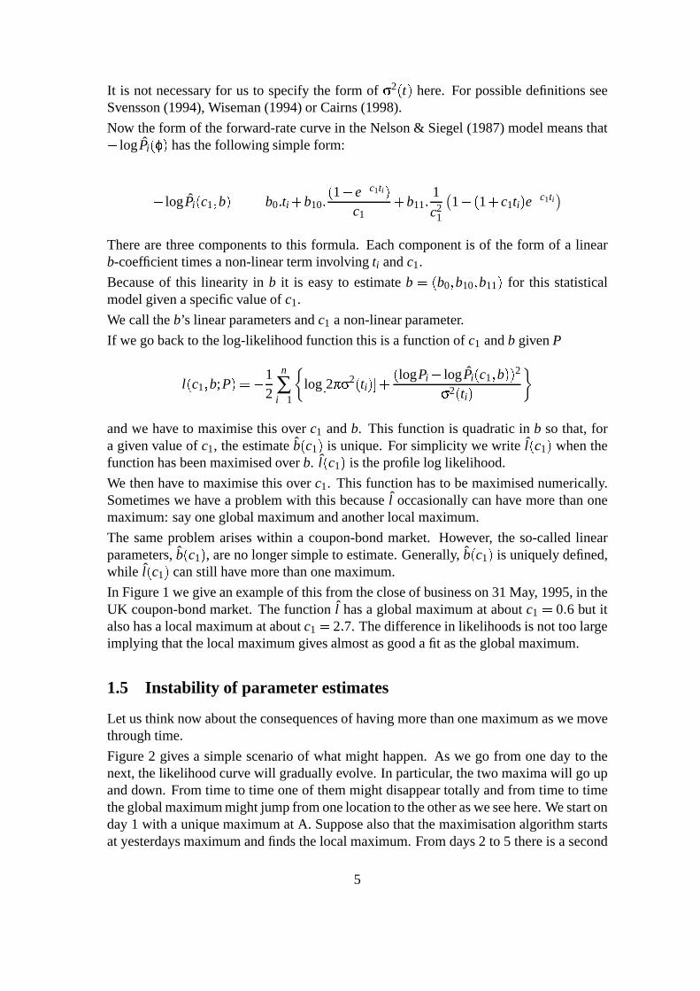
We then have to maximise this over c1. This function has to be maximised numerically.Sometimes we have a problem with this because l occasionally can have more than onemaximum: say one global maximum and another local maximum.

The same problem arises within a coupon-bond market. However, the so-called linearparameters, b c1 , are no longer simple to estimate. Generally, b c1 is uniquely defined,while l c1 can still have more than one maximum.

In Figure 1 we give an example of this from the close of business on 31 May, 1995, in theUK coupon-bond market. The function l has a global maximum at about c1 0 6 but italso has a local maximum at about c1 2 7. The difference in likelihoods is not too largeimplying that the local maximum gives almost as good a fit as the global maximum.

1.5 Instability of parameter estimates

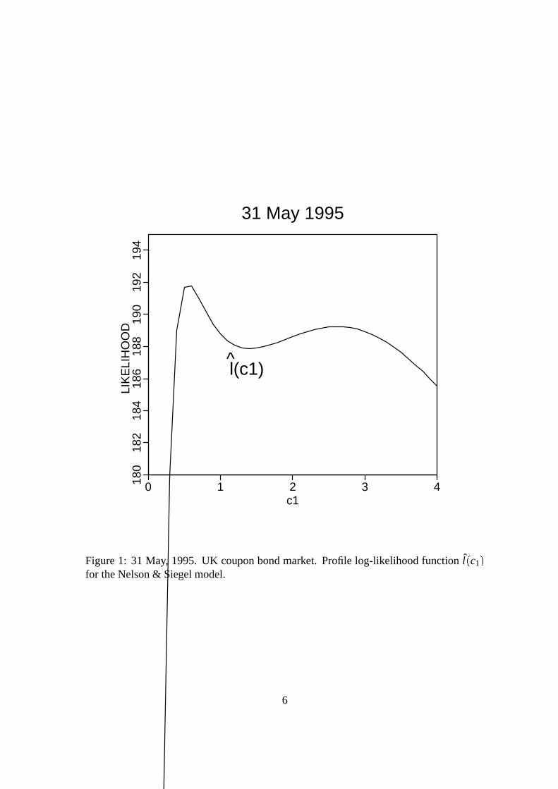
Let us think now about the consequences of having more than one maximum as we movethrough time.

Figure 2 gives a simple scenario of what might happen. As we go from one day to thenext, the likelihood curve will gradually evolve. In particular, the two maxima will go upand down. From time to time one of them might disappear totally and from time to timethe global maximum might jump from one location to the other as we see here. We start onday 1 with a unique maximum at A. Suppose also that the maximisation algorithm startsat yesterdays maximum and finds the local maximum. From days 2 to 5 there is a second

5

0 1 2 3 4c1

180

182

184

186

188

190

192

194

LIK

ELI

HO

OD

31 May 1995

l(c1)^

Figure 1: 31 May, 1995. UK coupon bond market. Profile log-likelihood function l c1

for the Nelson & Siegel model.

6

l(c1)^

Day 1

A

l(c1)^

Day 2

AB

l(c1)^

Day 3

AB

l(c1)^

Day 4

AB

l(c1)^

Day 5

AB

l(c1)^

Day 6

B

Figure 2: Possible development of the profile log-likelihood function through time.

7

maximum at B and indeed on days 3 and 5 this is the global maximum. The algorithm willcontinue until day 5, however, at maximum A. It is not until day 6 when the maximum atA disappears totally that the algorithm moves across to B. Other algorithms might jumpmore frequently, in particular if they are designed to find the global maximum.

What are the consequences of this problem?

We have identified that as we move from one day to the next the location of the maximummight jump. This is sometimes referred to as a catastrophic jump. When such a jumpoccurs, the size of the jump will typically be much larger than would be consistent withthe corresponding changes in prices. For example, if prices follow a diffusion process thenthe parameter estimates should also follow a diffusion process and in particular should bea continuous process: this continuity will clearly be violated if there is a catastrophicjump.

If parameter estimates jump then a published yield index will also jump in an equallyobvious way and the indices will start to lack credibility and fall into disuse. Equally ifthe curve is used as input to a Heath-Jarrow-Morton model with frequent recalibrationit is essential that the recalibrated curves evolve in a way which is consistent with pricechanges. This is not the case if catastrophic jumps occur which will cause unexpectedjumps, for example, in derivative prices.

The existence of more than one maximum can also lead to potential mispricing of suchthings as bonds, interest-rate derivatives or the pricing of annuities or other life insurancecontracts.

All of the Dobbie & Wilkie (1978), Svensson (1994) and Wiseman (1994) models exhibitthe same problem with multiple maxima (for example, see Cairns, 1998). In particular,this problem can arise in a zero-coupon bond market as well as in a coupon-bond market.In each case estimates for the linear, polynomial coefficients are unique and simple toderive while the multiple maxima show up in their profile log-likelihood functions. Theproblem arises on different dates, however, for different models and with varying degreesof magnitude.

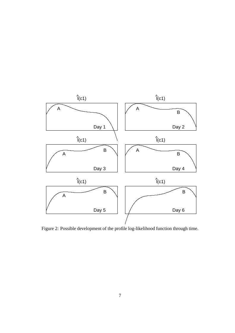
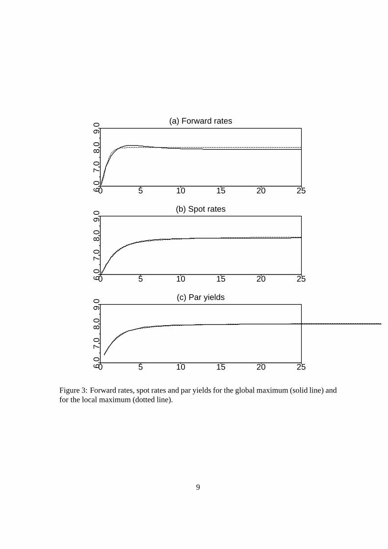
In Figure 3 we return to the previous example. Here we have plotted forward-rate, spot-rate and par-yield curves for each of the two maxima in Figure 1. The largest differencesoccur between the two forward-rate curves. This is because these rates are the furthestfrom what we actually observe: which is coupon-bond prices. Par yields are closest towhat we see on the market so the errors are smallest. The maximum difference here isabout only 0.03% which does not sound very much. But if we take the issue of a long-dated stock with a duration, say, of 10 years, then this leads to an error of £3 million per£1 billion issued, which is not trivial. On other dates and for other models these errorscan be bigger.

2 The restricted-exponential family

Given the shortcomings of the models described in the previous section, an alternativemodel is therefore appropriate. Here we describe the the restricted-exponential family.This is a simple family of forward-rate curves:

8

0 5 10 15 20 256.0

7.0

8.0

9.0 (a) Forward rates

0 5 10 15 20 256.0

7.0

8.0

9.0 (b) Spot rates

0 5 10 15 20 256.0

7.0

8.0

9.0 (c) Par yields

Figure 3: Forward rates, spot rates and par yields for the global maximum (solid line) andfor the local maximum (dotted line).

9

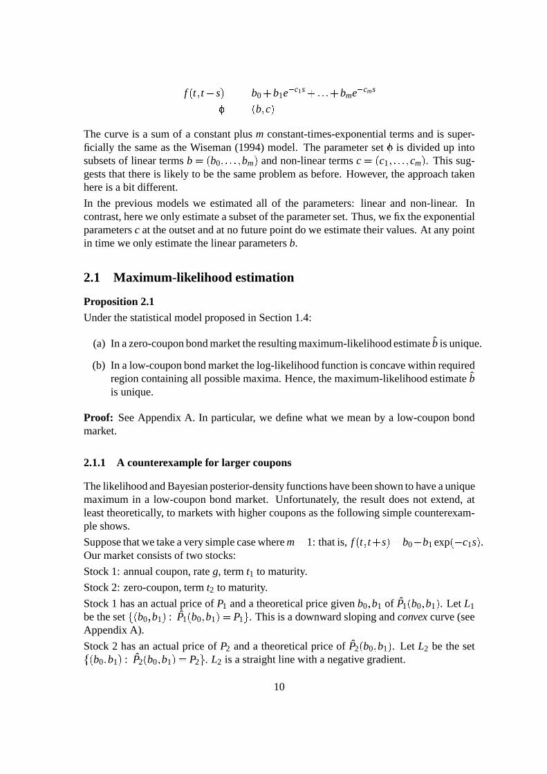
f t t s b0 b1e c1s bme cms

b c

The curve is a sum of a constant plus m constant-times-exponential terms and is super-ficially the same as the Wiseman (1994) model. The parameter set is divided up intosubsets of linear terms b b0 bm and non-linear terms c c1 cm . This sug-gests that there is likely to be the same problem as before. However, the approach takenhere is a bit different.

In the previous models we estimated all of the parameters: linear and non-linear. Incontrast, here we only estimate a subset of the parameter set. Thus, we fix the exponentialparameters c at the outset and at no future point do we estimate their values. At any pointin time we only estimate the linear parameters b.

2.1 Maximum-likelihood estimation

Proposition 2.1

Under the statistical model proposed in Section 1.4:

(a) In a zero-coupon bond market the resulting maximum-likelihood estimate b is unique.

(b) In a low-coupon bond market the log-likelihood function is concave within requiredregion containing all possible maxima. Hence, the maximum-likelihood estimate bis unique.

Proof: See Appendix A. In particular, we define what we mean by a low-coupon bondmarket.

2.1.1 A counterexample for larger coupons

The likelihood and Bayesian posterior-density functions have been shown to have a uniquemaximum in a low-coupon bond market. Unfortunately, the result does not extend, atleast theoretically, to markets with higher coupons as the following simple counterexam-ple shows.

Suppose that we take a very simple case where m 1: that is, f t t s b0 b1 exp c1s .Our market consists of two stocks:

Stock 1: annual coupon, rate g, term t1 to maturity.

Stock 2: zero-coupon, term t2 to maturity.

Stock 1 has an actual price of P1 and a theoretical price given b0 b1 of P1 b0 b1 . Let L1

be the set b0 b1 : P1 b0 b1 P1 . This is a downward sloping and convex curve (seeAppendix A).

Stock 2 has an actual price of P2 and a theoretical price of P2 b0 b1 . Let L2 be the setb0 b1 : P2 b0 b1 P2 . L2 is a straight line with a negative gradient.

10

Given the details of stock 1 it is possible to choose P2 and t2 such that L1 and L2 intersectin two points within the feasible region b : f t t s 0 for all s 0 . (Withm 2, b : b0 0 b0 b1 0 .) Let the points of intersection be b10 bb11 andb20 bb21 . At each point the theoretical prices equal the observed prices so clearly the

likelihood function will be maximised at both points of intersection. These maxima willalso, of course, be of the same height.

Numerical example:

Suppose that c1 0 2. For stock 1 we have P1 1, t1 20 and g 0 08, and for stock 2we have P2 0 352478, t2 13 3562.

The there are two solutions in b b0 b1 : b 0 03 0 137958 and b 0 11 0 091620 .

The experience of the UK gilts market suggests, however, that there is no problem withmultiple maxima. The counterexample above just shows that we cannot rule out the possi-bility altogether. This is possibly because the problem diminishes as the number of stocksincreases.

2.2 Bayesian estimation

2.2.1 Maximum-posterior-density estimation

Suppose instead we wish to use Bayesian methods with a prior distribution g b for b anda 0-1 loss function. Then the log-posterior density function is g b P g b l b;Pconstant, and the Bayesian estimator is the mode of the posterior distribution. (The 0-1loss function thus gives an estimator which gives the best fit which is consistent with theprior distribution.)

There are two principal reasons for using Bayesian methods:

We have introduced a constraint that the forward-rate curve should be positive atall maturities, on the basis that the risk-free rate will be non-negative at all times.If f t t s is equal to zero for any value of s then this means that r t s 0with probability 1. If we wish to exclude this possibility then we must require thatf t t s is strictly positive for all s. It is unreasonable to require that f t t s hasa minimum value higher than 0. However, if we use maximum likelihood and thisfinds that the maximum is at some b for which the forward-rate curve is negativeat some maturities then the introduction of a constraint will mean that the forward-rate curve is still equal to 0 for some s. This problem can be avoided if we useBayesian methods. In particular, if the prior density function, g b , tends to zeroon the boundary of the feasible region (in which f t t s remains positive) thenthe maximum of the posterior will give a strictly positive forward-rate curve at allmaturities.

Bayesian methods provide a coherent framework within which we can analyse pa-rameter risk and construct confidence intervals for specified interest rates and so

11

on.

Corollary 2.2

If the log-prior distribution function is concave then:

(a) In a zero-coupon bond market the resulting Bayesian estimate b is unique.

(b) In a low-coupon bond market the log-posterior density function is concave withinrequired region containing all possible maxima. Hence, the Bayesian estimate b isunique.

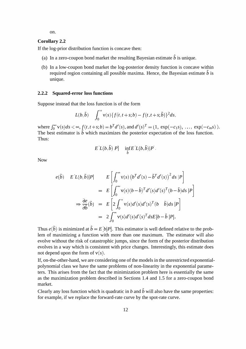
2.2.2 Squared-error loss functions

Suppose instead that the loss function is of the form

L b b0

s f t t s;b f t t s; b 2ds

where 0 s ds , f t t s;b bTd s , and d s T 1 exp c1s exp cms .The best estimator is b which maximizes the posterior expectation of the loss function.Thus:

E L b b P infb

E L b b P

Now

e b E L b b P E0

s bT d s bT d s2

ds P

E0

s b b T d s d s T b b ds P

e

bb E 2

0s d s d s T b b ds P

20

s d s d s T dsE b b P

Thus e b is minimized at b E b P . This estimator is well defined relative to the prob-lem of maximizing a function with more than one maximum. The estimator will alsoevolve without the risk of catastrophic jumps, since the form of the posterior distributionevolves in a way which is consistent with price changes. Interestingly, this estimate doesnot depend upon the form of s .

If, on-the-other-hand, we are considering one of the models in the unrestricted exponential-polynomial class we have the same problems of non-linearity in the exponential parame-ters. This arises from the fact that the minimization problem here is essentially the sameas the maximization problem described in Sections 1.4 and 1.5 for a zero-coupon bondmarket.

Clearly any loss function which is quadratic in b and b will also have the same properties:for example, if we replace the forward-rate curve by the spot-rate curve.

12

3 Further remarks

3.1 Choice of m

To get a consistently good fit in the UK gilts market we require m 4: that is, 4 expo-nential terms. Inevitably we require more terms than if we estimate both the linear andnon-linear parameters. The new approach with 4 exponential terms is roughly equivalentto estimating b and c in a model with only 2 exponential terms (but in each case we arestill only estimating 5 parameter values). However, the restricted exponential model hasthe advantage that it will fit much better on dates where more than one turning point inthe forward-rate curve is apparent.

With m 4 we can have a very rich or wide range of yield curves with up to 3 turningpoints.

3.2 Choice of c

The restricted-exponential fixes c at the outset. It is relevant, therefore, to ask the ques-tions what is an appropriate choice for c and what quantities are sensitive to the choice ofc?

One point that can be made at the outset is that it is reasonable to think of variation of theparameters c as variation within a continuous spectrum of models rather than parametervalues. Normally we consider a collection of models to be a discrete and possibly finitecollection. Here different values of c can be thought of as representing different models.

First, goodness of fit can be seen to be not sensitive to changes in c (Cairns, 1998). Onthe other hand, fitted very short and very long rates are sensitive. In between, fitted rateshardly vary if the value of c is changed. This, in fact, is an artefact of the data rather thanthe model since we are exptrapolating beyond the range of the data. The same would betrue of other models.

Other quantities, for example, swaps or spreads might be sensitive to the choice of c butthis is beyond the scope of this paper.

3.3 A more general family of curves

Bjørk and Christensen (1997) consider what families of curve are consistent with theevolution of certain models for the term structure. They describe a more general classof model: the restricted-exponential-polynomial family. Any curve in this family inwhich the polynomials are all of degree 0 is in the restricted-exponential family. A sim-ple example is the Vasicek (1977) model. This is a one-factor model under which theforward-rate curve evolves within the family of curves f t t s b0 b1 exp c1tb2 exp c2t b0 b1 b2 where c1 and c2 are fixed and c2 2c1. There are of course fur-ther restrictions on the parameters b0, b1 and b2 but the curve does evolve within thishigher-dimensional family.

13

Acknowledgements

The author has benefitted from conversations with many individuals: in particular, DavidWilkie, Geoff Chaplin, Andrew Smith, Gerry Kennedy, Freddy Delbaen and Julian Wise-man.

Part of this work was carried out while the author was in receipt of a grant from theFaculty and Institute of Actuaries.

14

References

1. BJØRK, T. AND CHRISTENSEN, B. J. Forward rate models and invariant mani-folds. Preprint, Stockholm School of Economics (1997)

2. CAIRNS, A.J.G. Uncertainty in the modelling process. Transactions of the 25thInternational Congress of Actuaries, Brussels 1, 67-94. (1995)

3. CAIRNS, A.J.G. Descriptive bond-yield and forward-rate models for the Britishgovernment securities’ market.. To appear in the British Actuarial Journal. (1998)

4. DALQUIST, M., AND SVENSSON, L.E.O. Estimating the term structure of interestrates for monetary policy analysis. Scandinavian Journal of Economics 98, 163-183 (1996)

5. DEACON, M., AND DERRY, A. Estimating the term structure of interest rates.Bank of England Working Paper Series Number 24 (1994)

6. DOBBIE, G.M. AND WILKIE, A.D. The FT-Actuaries Fixed Interest Indices.Journal of the Institute of Actuaries 105, 15-27 (1978) and Transactions of theFaculty of Actuaries 36:203-213.

7. FELDMAN, K.S., BERGMAN, B., CAIRNS, A.J.G., CHAPLIN, G.B., GWILT,G.D., LOCKYER, P.R., AND TURLEY, F.B. Report of the fixed interest work-ing group. To appear in the British Actuarial Journal (1998)

8. FLESAKER, B., AND HUGHSTON, L.P. Positive interest. Risk 9(1), 46-49(1996)

9. HEATH, D., JARROW, R. AND MORTON, A. Bond pricing and the term structureof interest rates: a new methodology for contingent claims valuation. Economet-rica 60, 77-105 (1992)

10. JARROW, R. Modelling Fixed Income Securities and Interest Rate Options. NewYork: McGraw-Hill 1996

11. MASTRONIKOLA, K. Yield curves for gilt-edged stocks: a new model. Discussionpaper number 49. Bank of England. (1991)

12. MCCULLOCH, J.H. Measuring the term structure of interest rates. Journal ofBusiness 44, 19-31 (1971)

13. MCCULLOCH, J.H. The tax-adjusted yield curve. Journal of Finance 30, 811-830 (1975)

14. MILLS, T.C. The Econometric Modelling of Financial Time Series. Cambridge:CUP 1993

15

15. NELSON, C.R., AND SIEGEL, A.F. Parsimonious modeling of yield curves. Jour-nal of Business 60, 473-489 (1987)

16. REBONATO, R. Interest Rate Option Models. Chichester: Wiley 1996

17. SVENSSON, L.E.O. Estimating and interpreting forward interest rates: Sweden1992-1994. Working paper of the International Monetary Fund 94.114, 33 pages(1994)

18. VASICEK, O. An equilibrium characterisation of the term structure. Journal ofFinancial Economics 5, 177-188 (1977)

19. VASICEK, O.E., AND FONG, H.G. Term structure modelling using exponentialsplines. Journal of Finance 37, 339-348 (1982)

20. WEI, W.W.S. Time Series Analysis. Redwood City: Addison-Wesley 1990

21. WISEMAN, J. The exponential yield curve model. J.P.Morgan, 16 December(1994)

16

Appendix A

A.1 Zero-coupon bond market

Define Z b; t Z b Z b; t exp bT d t where bT b0 bm , d t T d0 t dm t ,d0 t t and dk t 1 exp ckt ck for k 1 m.

For a bond maturing at ti write di d ti and dik dk ti .

Suppose that the observed prices are P1, P2, ..., PN . The likelihood function is

l b;P12

N

i 1log2 2 ti logPi logZ b; ti

2 2 ti

12

N

i 1i logPi dT

i b 2 constant

where i 1 2 ti

Maximising the likelihood is thus equivalent to minimising the function

g P b12

N

i 1i logPi dT

i b 2

d2gdb i

ididTi

The matrix of second derivatives is constant and positive definite.

Proposition 2.1(a)

Hence g P b is convex and has a unique minimum in b.

If we wish instead to use Bayesian methods it is necessary for us to specify also a priordensity function. Suppose that the log-prior density function is denoted by p b . Thelog-posterior density function is then

p b P p b g P b constant

Corollary 2.2(a)

If p b is convex then 2 p b b2 is positive semi-definite. Thus the matrix of secondderivatives of minus the log-posterior density function 2 p b P b2 is positive definiteand there is a unique value of b for which p b P b 0.

A.2 Coupon-bond market

Suppose that there are N bonds each with a nominal value of 1. Bond i has cashflowsci1 cini at times 0 ti1 tini respectively. Given b, the theoretical price of eachbond is then:

17

Pi bni

j 1ci jZ b; ti j

ni

j 1ci j exp bT d ti j

Write di j d ti j

di jk dk ti j

g b12

N

i 1i logPi log

ni

j 1ci jZ b; ti j

2

(Recall that the log-likelihood is l b;P g b constant.)

Now

Z b; t exp bT d tdZ b; t

dbZ b; t d t

d2Z b; tdb2 Z b; t d t d t T

Thus g bi

i logPi logj

ci jZ b; ti jj ci j

dZ b;ti jdb

j ci jZ b; ti j

ii logPi log

jci jZ b; ti j

jfi j b di j

ii logPi log

jci jZ b; ti j di b

where di bj

fi j b di j

and fi j bci jZ b; ti j

j ci jZ b; ti j

g bi

ij ci j

dZ b;ti jdb

j ci jZ b; ti j

j ci jdZ b;ti j

db

j ci jZ b; ti j

T

ii logPi log

jci jZ b; ti j Vi b

iibi b bi b T

ii logPi log

jci jZ b; ti j Vi b

where Vi bddb

j ci jdZ b;ti j

db

j ci jZ b; ti j

j ci jZ b; ti j di jdTi j j ci jZ b; ti j j ci jZ b; ti j di j j ci jZ b; ti j dT

i j

j ci jZ b; ti j2

jfi j b di jd

Ti j

jfi j b di j

jfi j b di j

T

18

jfi j b di j di b di j di b T

0

Now write Xi b logPi log j ci jZ b; ti j log Pi Pi b .

g bi

iXi b di b

g bi

i di b di b T Xi b Vi b

Now in a zero-coupon bond market Vi b 0 and the di b are constant and do not dependon b. Thus g b is constant and positive definite confirming the simpler derivation above.

A.3 Assumptions

We make the following assumptions:

The range of acceptable values for b is denoted by . Each b must satisfy the fol-lowing criterion: for all 0 t s, 1 Z b; t Z b;s . This criterion is equivalent tothe assumption that the forward-rate curve f t t s is non-negative for all t and for alls 0: that is,

b : bT d t 0 for all t

where d t T 1 exp c1t exp cmt

Suppose that u 0 and that b . For any 0 t s we note that 1 Z b; t Z b;sand therefore 0 bT d t bT d s . Thus

0 u bT d t u bT d s

1 exp ubT d t exp ubT d s

1 Z bu; t Z bu;s

Thus b if and only if bu for all u 0. That is, is a cone.

Furthermore, suppose that bA and bB are in . Then for any such that 0 1, andfor any 0 t s:

0 bTAd t bAd s

and 0 bTBd t bBd s

0 1 bTAd t bT

Bd t 1 bTAd s bT

Bd s

0 1 bA bBT d t 1 bA bB

T d s

1 bA bB

Thus is a convex cone.

19

A.4 Locality of possible minima

We define the following sets:

B0 b : Pi Pi b for all i

B1 b : Pi Pi b for all i

B2 B1

Clearly for all b B0, Pi bs Pi for all 0 s 1. That is, b B0 implies that bs B0

for all 0 s 1.

Similarly, b B1 implies that bs B1 for all 1 s .

Lemma A.1

There does not exist b B0 or b B1 such that g b 0 is positive definite.

Proof Suppose that there exists such a b B1.

Let s0 inf s : bs B1 . Thus Pi bs Pi for all s s0 and Pi bs is decreasing with sfor s s0. Hence g bs is an increasing function of s for s s0 which indicates that therecannot be a minimum at b.

Similarly there does not exist such a b B0.

Lemma A.2

B1 is convex.

Proof

Note that Pi b is convex in b for all i.

Suppose bA and bB are members of B1.

Then Pi bA Pi and Pi bB Pi.

For 0 1: since Pi b is convex,

Pi 1 bA bB 1 Pi bA Pi bB Pi

Thus bA bB B1 1 bA bB B1.

Given bA bB B1 this is true for all i. Thus B1 is convex.

Proposition 2.1(b)

For small coupon rates there is a unique maximum.

Proof

We proceed as follows:

(a) Establish a means of moving continuously and smoothly from zero-coupon bonds, viaa new parameter, ( 0 giving a zero-coupon bond market and 1 giving us the truecoupon-bond market).

(b) Establish that B2 B1 is finite, and let B3 be some finite expansion of B2 and whichcontains B2 for all values of : 0 1.

20

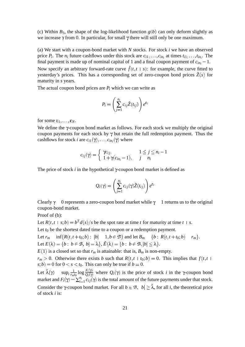
(c) Within B3, the shape of the log-likelihood function g b can only deform slightly aswe increase from 0. In particular, for small there will still only be one maximum.

(a) We start with a coupon-bond market with N stocks. For stock i we have an observedprice Pi. The ni future cashflows under this stock are ci1 cini at times ti1 tini . Thefinal payment is made up of nominal capital of 1 and a final coupon payment of cini 1.

Now specify an arbitrary forward-rate curve f t t s : for example, the curve fitted toyesterday’s prices. This has a corresponding set of zero-coupon bond prices Z s formaturity in s years.

The actual coupon bond prices are Pi which we can write as

Pi

ni

j 1ci jZ ti j e i

for some 1 N.

We define the -coupon bond market as follows. For each stock we multiply the originalcoupon payments for each stock by but retain the full redemption payment. Thus thecashflows for stock i are ci1 cini where

ci jci j 1 j ni 1

1 cini 1 j ni

The price of stock i in the hypothetical -coupon bond market is defined as

Qi

ni

j 1ci j Z ti j e i

Clearly 0 represents a zero-coupon bond market while 1 returns us to the originalcoupon-bond market.

Proof of (b):

Let R t t s;b bT d s s be the spot rate at time t for maturity at time t s.

Let t0 be the shortest dated time to a coupon or a redemption payment.

Let rm inf R t t t0;b : b 1 b and let Bm b : R t t t0;b rm .

Let E b : b b , E b : b b .

E 1 is a closed set so that rm is attainable: that is, Bm is non-empty.

rm 0. Otherwise there exists b such that R t t t0;b 0. This implies that f t ts;b 0 for 0 s t0. This can only be true if b 0.

Let ˜ supi1

rmt0log Fi

Qiwhere Qi is the price of stock i in the -coupon bond

market and Finii 1 ci j is the total amount of the future payments under that stock.

Consider the -coupon bond market. For all b b ˜ , for all i, the theoretical priceof stock i is:

21

Qi bni

j 1ci j exp R t t ti j;b ti j

ni

j 1ci j exp R t t ti j;b b ti j b

ni

j 1ci j exp rmt0 b

Fi exp rmt0˜

Qi

Thus B2 B1 E ˜ .

Choose some such that sup0 1˜ .

Let B3 E .

Write g b for the log-likelihood function for the -coupon bond market.

Clearly g b is infinitely differentiable.

For any (0 1), for any i and for any b B3, Qi b Qi .

Thus, by Lemma A.1, there can be no b outside E such that g b b 0 at b.Hence no local maxima can come sliding in from infinity as soon as 0.

Let b B3 be the unique value of b such that

gb

b 0 0

Note that 2g b2 b 0 is constant and strictly positive definite. (This leads to theunique maximum b mentioned above for the zero-coupon bond market.)

Hence there exists 1 0 such that 2g b2 b is strictly positive definite for all0 1 and for all b B3 (since g is C and B3 is finite).

Thus for each (0 1) there is a unique b B3 (and hence ) which maximisesg b .

Corollary 2.2(b)

Furthermore, if a prior distribution for b is such that -1 times the log-prior density func-tion is positive semi-definite then -1 times the log-posterior density function is also posi-tive definite within B3.

22