sro.sussex.ac.uksro.sussex.ac.uk/id/eprint/70716/1/parmar, kiresh.pdfsro.sussex.ac.uk
TRANSCRIPT

A University of Sussex PhD thesis
Available online via Sussex Research Online:
http://sro.sussex.ac.uk/
This thesis is protected by copyright which belongs to the author.
This thesis cannot be reproduced or quoted extensively from without first obtaining permission in writing from the Author
The content must not be changed in any way or sold commercially in any format or medium without the formal permission of the Author
When referring to this work, full bibliographic details including the author, title, awarding institution and date of the thesis must be given
Please visit Sussex Research Online for more information and further details

Time-Delayed Models of Genetic
Regulatory Networks
Kiresh Parmar
A thesis submitted for the degree of Doctor of Philosophy
School of Mathematical and Physical Sciences
University of Sussex
March 2017

Declaration
I hereby declare that this thesis has not been, and will not be, submitted in whole or in
part to another University for any other academic award. I also declare that this thesis
was composed by myself and that the work contained therein is my own, except where
explicitly stated otherwise.
Signature ..........................................................................
Kiresh Parmar
i

Acknowledgements
First and foremost I would like to thank my incredible supervisors, Dr Yuliya Kyrychko
and Dr Konstantin Blyuss, whose encouragement during my undergraduate degree gave me
the confidence to pursue a PhD. I am grateful for their guidance and support throughout
this research and I am so happy to have chosen them as my MMath project supervisors
back in 2012.
I would also like to thank Dr Stephen John Hogan whom I collaborated with, alongside
my supervisors, on my paper.
A special thanks goes to the University of Sussex Mathematics department for funding
my PhD. The staff and faculty have made my 8 years at Sussex a memorable experience.
I am eternally grateful to have such an amazing wife, who keeps me calm and focussed.
I am blessed to have my Mum, Dad, and brother, who have all helped me along this journey.
My thanks also extends to my in-laws and all of my family and friends, who have
encouraged and inspired me. In particular, I would like to thank Charlie, whose support
has been invaluable throughout my time at Sussex.
ii

Abstract
In this thesis I have analysed several mathematical models, which represent the dynamics
of genetic regulatory networks. Methods of bifurcation analysis and direct numerical
simulations were employed to study the biological phenomena that can occur due to the
presence of time delays, such as stable periodic oscillations induced by Hopf bifurcations.
To highlight the biological implications of time-delayed systems, different models of genetic
regulatory networks as relevant to the onset and development of cancer were studied in
detail, as well as genetic regulatory networks which describe the effects of transcription
factors in the immune system. A network of an oscillator coupled with a switch was
explored, as systems such as these are prevalent in genetic regulatory networks. The
effects of time delays on its oscillatory and bistable behaviour were then investigated, the
results of which were compared with available results from the literature.
iii
Contents
Acknowledgements ii
Abstract iii
List of Figures vi
Preface xiv
1 Introduction 1
1.1 Literature Review . . . . . . . . . . . . . . . . . . . . . . . . . . . . . . . . 2
1.1.1 Mathematical Models of Gene Regulatory Networks . . . . . . . . . 2
1.1.2 Delay Differential Equations . . . . . . . . . . . . . . . . . . . . . . . 7
1.1.3 Autoinhibition Model with Transcriptional Delay . . . . . . . . . . . 11
1.2 Thesis Outline . . . . . . . . . . . . . . . . . . . . . . . . . . . . . . . . . . 19
2 Time-Delayed Models of Gene Regulatory Networks 21
2.1 Time-Delayed Models: Derivation and Positivity . . . . . . . . . . . . . . . 22
2.2 Analysis of the Delayed Simplified Nonlinear Model (DSNM) . . . . . . . . 27
2.3 Analysis of the Delayed Complete Nonlinear Model (DCNM) . . . . . . . . 33
2.4 Discussion . . . . . . . . . . . . . . . . . . . . . . . . . . . . . . . . . . . . . 37
3 Time-Delayed Model of a Genetic Regulatory Network in the Immune
System 40
3.1 Derivation of the Time-Delayed Model . . . . . . . . . . . . . . . . . . . . . 42
3.2 Time Delayed Model: Positivity and Steady States . . . . . . . . . . . . . . 45
3.3 Analysis of the Delayed Repressilator with Auto-activation Model (DRAM) 47
3.3.1 Stability of Steady States with a Zero Component . . . . . . . . . . 48
iv

3.3.2 Stability of Steady States with Non-zero Components . . . . . . . . 54
3.4 Discussion . . . . . . . . . . . . . . . . . . . . . . . . . . . . . . . . . . . . . 70
4 Time-Delayed Model of a Genetic Network with Switches and Oscilla-
tions 71
4.1 The Delayed Model . . . . . . . . . . . . . . . . . . . . . . . . . . . . . . . . 73
4.2 Time Delayed Model: Positivity and Steady States . . . . . . . . . . . . . . 77
4.3 Analysis of the Delayed Repressilator Coupled with Toggle Switch Model . 80
4.3.1 The Effect of Delays in the Toggle Switch . . . . . . . . . . . . . . . 82
4.3.2 The Effect of Delays in the Repressilator . . . . . . . . . . . . . . . . 84
4.4 Oscillatory Behaviour of the DDE System . . . . . . . . . . . . . . . . . . . 86
4.5 Discussion . . . . . . . . . . . . . . . . . . . . . . . . . . . . . . . . . . . . . 91
5 Discussion and Future Work 92
5.1 Summary and Conclusions . . . . . . . . . . . . . . . . . . . . . . . . . . . . 92
5.2 Future Research . . . . . . . . . . . . . . . . . . . . . . . . . . . . . . . . . 94
Bibliography 96
v

List of Figures
1.1 Network motif for the auto-inhibitory gene, X, of the Zebrafish somite seg-
mentation clock. The node is gene X and the loop represents regulation of
mRNA production by self-inhibition. . . . . . . . . . . . . . . . . . . . . . . 12
1.2 Stability boundary of the steady state (p, m) of system (1.11). The steady
state is stable below the surface in (a) and to the left of the boundary curves
shown in (b). Parameter values are c = 0.23, k = 33, and p0 = 40. . . . . . 16
1.3 Numerical solution of system (1.11): (a) τ = 5; (b) τ = 7. Parameter values
are a = 5, b = 0.7, c = 0.23, k = 33, and p0 = 40. The critical time delay
is τ0 = 6.1271. . . . . . . . . . . . . . . . . . . . . . . . . . . . . . . . . . . . 17
1.4 Stability boundary of the steady state (p, m) of system (1.11). The steady
state is stable below the surface in (a) and to the left of the boundary curves
shown in (b). Parameter values are a = 4.5, c = 0.23, and p0 = 40. . . . . . 18
1.5 Stability boundary of the steady state (p, m) of system (1.11). The steady
state is stable below the surface in (a) and to the left of the boundary curves
shown in (b). Parameter values are b = c = 0.23, and p0 = 40. . . . . . . . . 19
2.1 Hill functions for activation and inhibition of transcription in system (2.1),
varying the Hill coefficient, n. (a) Activation function. (b) Inhibition function. 23
2.2 Network motif for the activation-inhibition model of the DCNM and DSNM.
The nodes are genes A and B where expression of gene B is inhibited by
gene A, whilst expression of gene A is activated by gene B. . . . . . . . . . 25
2.3 Stability boundary of the steady state (pa, pb) of DSNM system (2.8). The
steady state is stable below the surface in (a) and to the left of the boundary
curves shown in (b). Parameter values are ma = mb = 2.35, θa = θb = 0.21,
na = nb = 3, and ka = kb = γa = γb = 1. . . . . . . . . . . . . . . . . . . . . 30
vi

2.4 Stability boundary of the steady state (pa, pb) of DSNM system (2.8). The
steady state is stable below the surface in (a) and (c) and to the left of the
boundary curves shown in (b) and (d). Parameter values are ma = mb =
2.35, na = nb = 3, and ka = kb = δa = δb = γa = γb = 1. . . . . . . . . . . . 31
2.5 Stability boundary of the steady state (pa, pb) of DSNM system (2.8). The
steady state is stable below the surface in (a), and to the left of the boundary
curves shown in (b). Parameter values are θa = θb = 0.21, na = nb = 3,
and ka = kb = δa = δb = γa = γb = 1. . . . . . . . . . . . . . . . . . . . . . 32
2.6 Numerical solution of DSNM system (2.8): (a) τ = 0.5; (b) τ = 2. Pa-
rameter values are ma = mb = 2.35, θa = θb = 1, na = nb = 3, and
ka = kb = δa = δb = γa = γb = 1. The critical time delay is τ0 = 0.9762. . . 32
2.7 Stability boundary of the steady state (ra, rb, pa, pb) of DCNM system (2.3).
The steady state is stable below the surface in (a), (c), and below the
boundary curves shown in (b), (d). Parameter values: θa = θb = 0.21,
na = nb = 3 and ka = kb = δa = δb = γa = γb = 1. . . . . . . . . . . . . . . 37
2.8 Numerical solution of DCNM system (2.3): (a) τ = 0.25; (b) τ = 2. Pa-
rameter values: ma = 0.6, mb = 0.3, θa = θb = 0.21, na = nb = 3, and
ka = kb = δa = δb = γa = γb = 1. The critical time delay is τ0 = 0.5314. . . 38
3.1 Network motif of the Repressilator with auto-activation model. The nodes
are genes X, Y, and Z, which are connected by edges, in red, representing
regulation of each gene by inhibition from the preceding gene in the cycle.
The loops, in blue, represent self activation of each gene. . . . . . . . . . . . 43
3.2 Numerical solution of three-gene Repressilator model with auto-activation
and without time delays. Parameter values: τx = τy = τz = 0, α1 = 4,
α2 = 5, α3 = 6, b1 = 4, b2 = 3, b3 = 1, c1 = 8, c2 = 10, c3 = 15, d1 = 0.5,
d2 = 2, d3 = 0.2, γ2 = 0.8, γ3 = 2. . . . . . . . . . . . . . . . . . . . . . . . . 44
vii
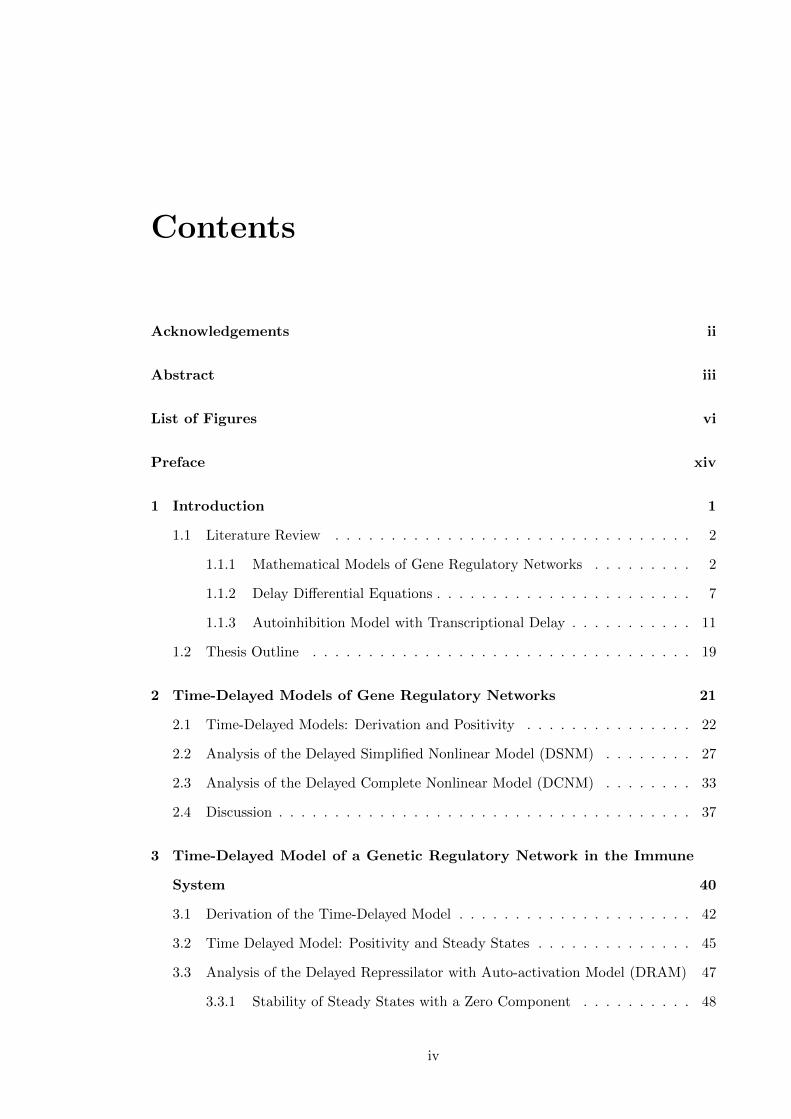
3.3 Parameter regions for stable and unstable steady states of DRAM sys-
tem (3.4). Each colour coded number is the indice of the corresponding
steady state which is stable in that region, whilst all other steady states
are unstable or infeasible. The blue region labelled 0 is where all steady
states are unstable, leading to sustained oscillations. Parameter values:
τx = τy = τz = 0, α3 = 6, b1 = 4, b2 = 3, b3 = 1, c1 = 8, c2 = 10, c3 = 15,
d1 = 0.5, d2 = 2, d3 = 0.2, γ2 = 0.8, γ3 = 2. . . . . . . . . . . . . . . . . . . 50
3.4 Numerical solutions of DRAM system (3.4): (a) α1 = 13. (b) α1 = 25.
Parameter values: τx = τy = τz = 0, α2 = 17, α3 = 6, b1 = 4, b2 = 3,
b3 = 1, c1 = 8, c2 = 10, c3 = 15, d1 = 0.5, d2 = 2, d3 = 0.2, γ2 = 0.8, γ3 = 2. 51
3.5 Parameter regions for stable and unstable steady states of DRAM sys-
tem (3.4). Each colour coded number is the indice of the corresponding
steady state which is stable in that region, whilst all other steady states
are unstable or infeasible. The blue region labelled 0 is where all steady
states are unstable, leading to sustained oscillations. Parameter values:
τx = τy = τz = 0, α1 = 4, α2 = 5, α3 = 6, b1 = 4, b2 = 3, b3 = 1, c3 = 15,
d1 = 0.5, d2 = 2, d3 = 0.2, γ2 = 0.8, γ3 = 2. . . . . . . . . . . . . . . . . . . 52
3.6 Parameter regions for stable and unstable steady states of DRAM sys-
tem (3.4). Each colour coded number is the indice of the corresponding
steady state which is stable in that region, whilst all other steady states
are unstable or infeasible. The blue region labelled 0 is where all steady
states are unstable, leading to sustained oscillations. Parameter values:
τx = τy = τz = 0, α1 = 4, α2 = 5, α3 = 6, b1 = 4, b2 = 3, b3 = 1, c1 = 8,
c2 = 10, c3 = 15, d3 = 0.2, γ2 = 0.8, γ3 = 2. . . . . . . . . . . . . . . . . . . 52
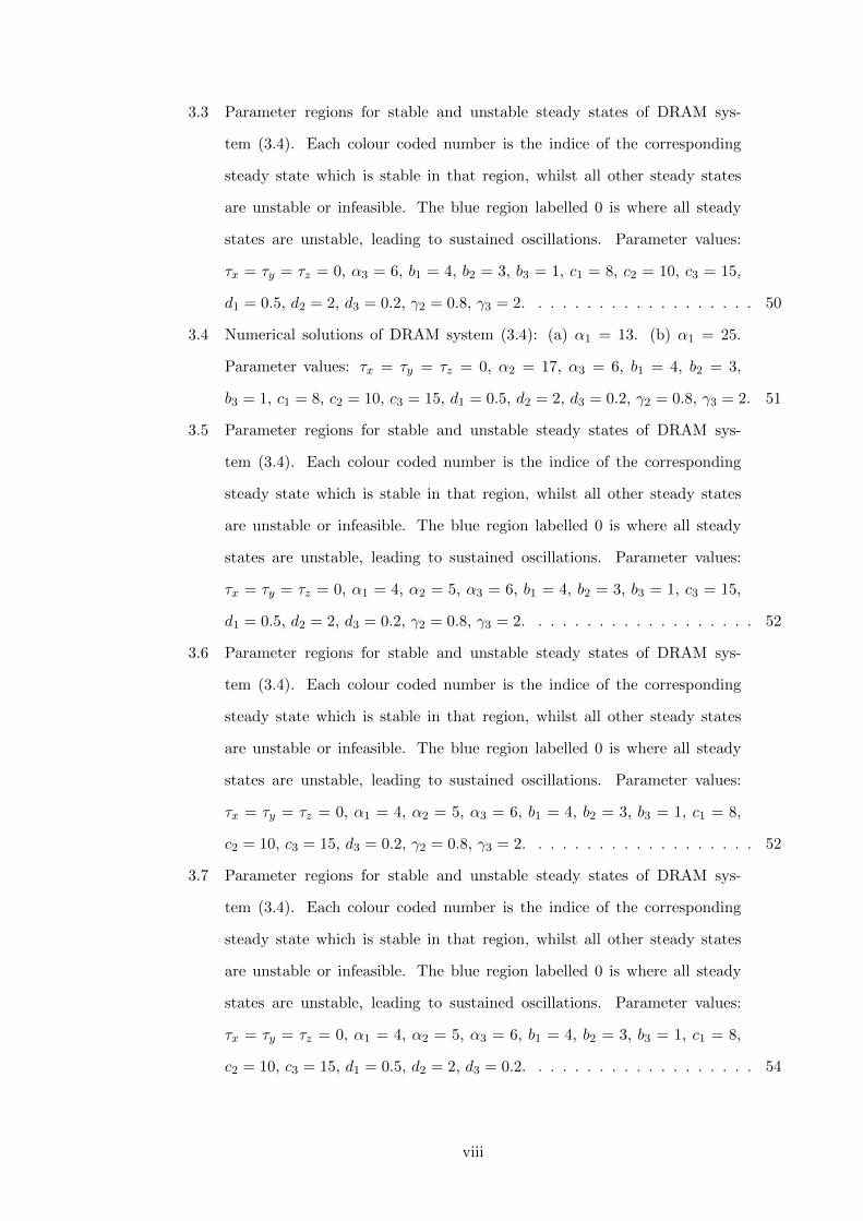
3.7 Parameter regions for stable and unstable steady states of DRAM sys-
tem (3.4). Each colour coded number is the indice of the corresponding
steady state which is stable in that region, whilst all other steady states
are unstable or infeasible. The blue region labelled 0 is where all steady
states are unstable, leading to sustained oscillations. Parameter values:
τx = τy = τz = 0, α1 = 4, α2 = 5, α3 = 6, b1 = 4, b2 = 3, b3 = 1, c1 = 8,
c2 = 10, c3 = 15, d1 = 0.5, d2 = 2, d3 = 0.2. . . . . . . . . . . . . . . . . . . 54
viii

3.8 Parameter regions for stable and unstable steady states of SDRAM system
(3.11). Each colour coded number is the indice of the corresponding steady
state which is stable in that region, whilst all other steady states are unsta-
ble or infeasible. The blue region labelled 0 is where all steady states are
unstable, leading to sustained oscillations. (b) is a magnified view of (a).
Parameter values: τ2 = 0, α2 = 5, α3 = 6, b1 = 4, b2 = 3, b3 = 1, c1 = 8,
c2 = 10, c3 = 15, d1 = 0.5, d2 = 2, d3 = 0.2, γ2 = 0.8, γ3 = 2. . . . . . . . . 59
3.9 Parameter regions for stable and unstable steady states of SDRAM system
(3.11). Each colour coded number is the indice of the corresponding steady
state which is stable in that region, whilst all other steady states are un-
stable or infeasible. The blue region labelled 0 is where all steady states
are unstable, leading to sustained oscillations. Parameter values: τ2 = 15,
α2 = 5, α3 = 6, b1 = 4, b2 = 3, b3 = 1, c1 = 8, c2 = 10, c3 = 15, d1 = 0.5,
d2 = 2, d3 = 0.2, γ2 = 0.8, γ3 = 2. . . . . . . . . . . . . . . . . . . . . . . . . 66
3.10 Parameter regions for stable and unstable steady states of SDRAM system
(3.11). Each colour coded number is the indice of the corresponding steady
state which is stable in that region, whilst all other steady states are un-
stable or infeasible. The blue region labelled 0 is where all steady states
are unstable, leading to sustained oscillations. Parameter values: τ2 = 15,
α1 = 4, α2 = 5, α3 = 6, b1 = 4, b2 = 3, b3 = 1, c2 = 10, c3 = 15, d1 = 0.5,
d2 = 2, d3 = 0.2, γ2 = 0.8, γ3 = 2. . . . . . . . . . . . . . . . . . . . . . . . . 67
3.11 Parameter regions for stable and unstable steady states of SDRAM system
(3.11). Each colour coded number is the indice of the corresponding steady
state which is stable in that region, whilst all other steady states are un-
stable or infeasible. The blue region labelled 0 is where all steady states
are unstable, leading to sustained oscillations. Parameter values: τ2 = 15,
α1 = 4, α2 = 5, α3 = 6, b1 = 4, b2 = 3, b3 = 1, c1 = 8, c2 = 10, c3 = 15,
d2 = 2, d3 = 0.2, γ2 = 0.8, γ3 = 2. . . . . . . . . . . . . . . . . . . . . . . . . 68
ix

3.12 The values of Max(Re(λ)) in the (τ1, τ2) parameter space for steady state
(x9, y9, z9) of SDRAM system. All other steady states are either unstable
or infeasible for these parameter schemes. (a) Parameter values: α1 = 4,
α2 = 5, α3 = 6, b1 = 4, b2 = 3, b3 = 1, c1 = 8, c2 = 10, c3 = 15, d1 = 0.5,
d2 = 2, d3 = 0.2, γ2 = 0.8, γ3 = 2. (b) α1 = 2. (c) c1 = 1. (d) d1 = 2.4. All
other parameters remain the same as (a) in (b)-(d). . . . . . . . . . . . . . . 69
4.1 Network motif of the Repressilator coupled with a Toggle switch. The nodes
are genes G1, G2, and G3 of the Repressilator, which are connected by
edges, in red, representing regulation of each gene by inhibition from the
preceding gene in the cycle. The genes X and Y of the Toggle switch are
connected by edges, in red, representing regulation of each gene by mutual
repression. The Repressilator and Toggle switch are coupled through an
edge, in blue, connecting gene G1 with X which represents regulation of
gene X by activation from G1. . . . . . . . . . . . . . . . . . . . . . . . . . . 74
x
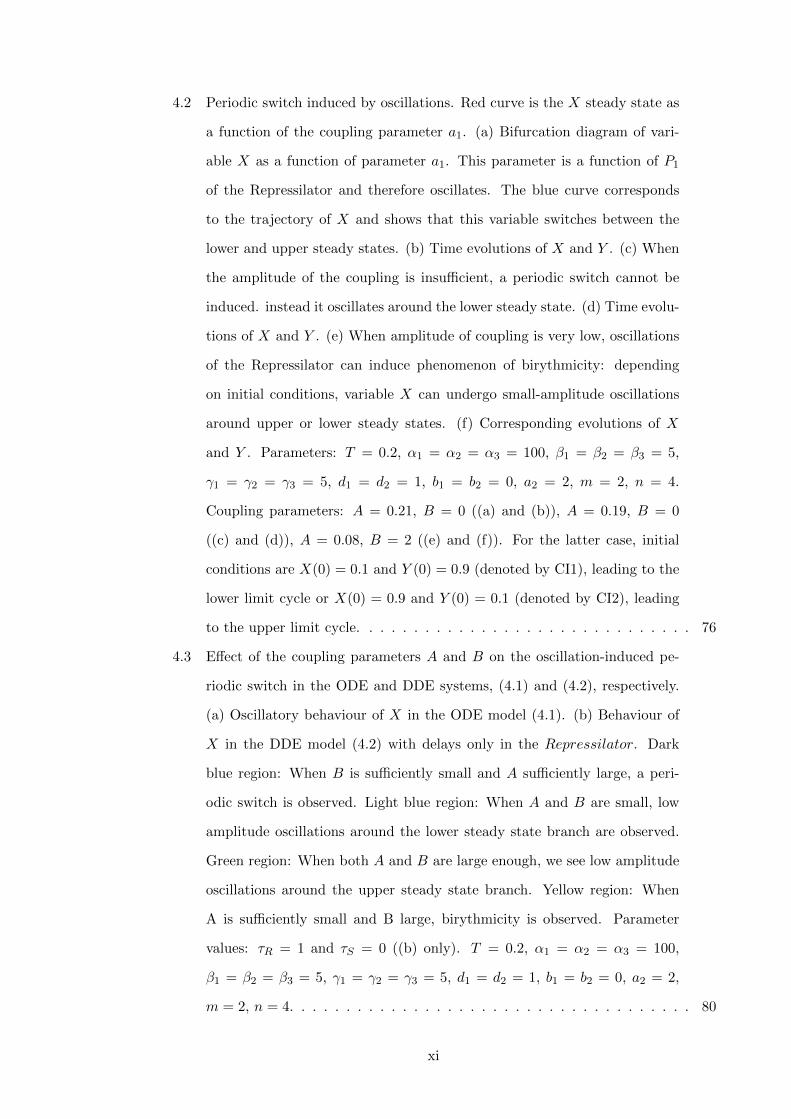
4.2 Periodic switch induced by oscillations. Red curve is the X steady state as
a function of the coupling parameter a1. (a) Bifurcation diagram of vari-
able X as a function of parameter a1. This parameter is a function of P1
of the Repressilator and therefore oscillates. The blue curve corresponds
to the trajectory of X and shows that this variable switches between the
lower and upper steady states. (b) Time evolutions of X and Y . (c) When
the amplitude of the coupling is insufficient, a periodic switch cannot be
induced. instead it oscillates around the lower steady state. (d) Time evolu-
tions of X and Y . (e) When amplitude of coupling is very low, oscillations
of the Repressilator can induce phenomenon of birythmicity: depending
on initial conditions, variable X can undergo small-amplitude oscillations
around upper or lower steady states. (f) Corresponding evolutions of X
and Y . Parameters: T = 0.2, α1 = α2 = α3 = 100, β1 = β2 = β3 = 5,
γ1 = γ2 = γ3 = 5, d1 = d2 = 1, b1 = b2 = 0, a2 = 2, m = 2, n = 4.
Coupling parameters: A = 0.21, B = 0 ((a) and (b)), A = 0.19, B = 0
((c) and (d)), A = 0.08, B = 2 ((e) and (f)). For the latter case, initial
conditions are X(0) = 0.1 and Y (0) = 0.9 (denoted by CI1), leading to the
lower limit cycle or X(0) = 0.9 and Y (0) = 0.1 (denoted by CI2), leading
to the upper limit cycle. . . . . . . . . . . . . . . . . . . . . . . . . . . . . . 76
4.3 Effect of the coupling parameters A and B on the oscillation-induced pe-
riodic switch in the ODE and DDE systems, (4.1) and (4.2), respectively.
(a) Oscillatory behaviour of X in the ODE model (4.1). (b) Behaviour of
X in the DDE model (4.2) with delays only in the Repressilator. Dark
blue region: When B is sufficiently small and A sufficiently large, a peri-
odic switch is observed. Light blue region: When A and B are small, low
amplitude oscillations around the lower steady state branch are observed.
Green region: When both A and B are large enough, we see low amplitude
oscillations around the upper steady state branch. Yellow region: When
A is sufficiently small and B large, birythmicity is observed. Parameter
values: τR = 1 and τS = 0 ((b) only). T = 0.2, α1 = α2 = α3 = 100,
β1 = β2 = β3 = 5, γ1 = γ2 = γ3 = 5, d1 = d2 = 1, b1 = b2 = 0, a2 = 2,
m = 2, n = 4. . . . . . . . . . . . . . . . . . . . . . . . . . . . . . . . . . . . 80
xi
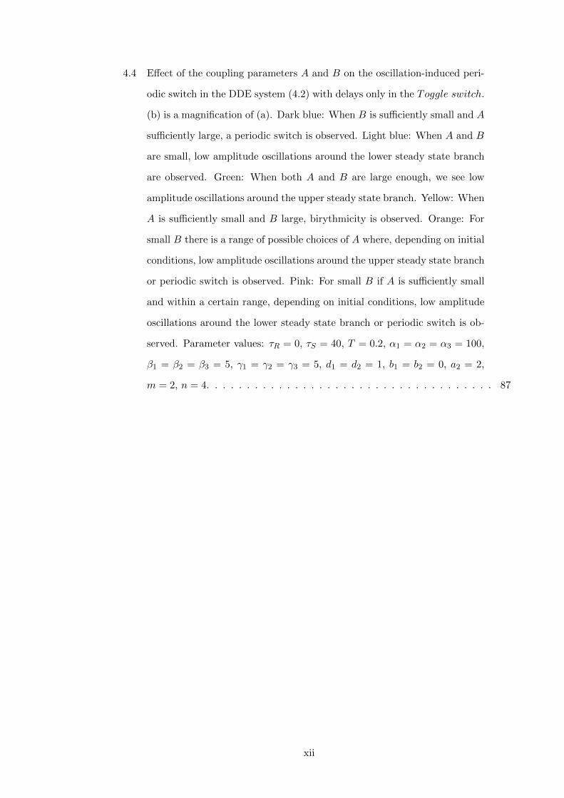
4.4 Effect of the coupling parameters A and B on the oscillation-induced peri-
odic switch in the DDE system (4.2) with delays only in the Toggle switch.
(b) is a magnification of (a). Dark blue: When B is sufficiently small and A
sufficiently large, a periodic switch is observed. Light blue: When A and B
are small, low amplitude oscillations around the lower steady state branch
are observed. Green: When both A and B are large enough, we see low
amplitude oscillations around the upper steady state branch. Yellow: When
A is sufficiently small and B large, birythmicity is observed. Orange: For
small B there is a range of possible choices of A where, depending on initial
conditions, low amplitude oscillations around the upper steady state branch
or periodic switch is observed. Pink: For small B if A is sufficiently small
and within a certain range, depending on initial conditions, low amplitude
oscillations around the lower steady state branch or periodic switch is ob-
served. Parameter values: τR = 0, τS = 40, T = 0.2, α1 = α2 = α3 = 100,
β1 = β2 = β3 = 5, γ1 = γ2 = γ3 = 5, d1 = d2 = 1, b1 = b2 = 0, a2 = 2,
m = 2, n = 4. . . . . . . . . . . . . . . . . . . . . . . . . . . . . . . . . . . . 87
xii

4.5 Oscillatory behaviour in the DDE model (4.2). (a) Bifurcation diagram of
variable X as a function of parameter a1. The blue curve shows that this
variable switches between the lower and upper steady states, with different
dynamics than seen in the ODE model (4.1). (b) Time evolutions of X
and Y . (c) When amplitude of coupling is insufficient, a periodic switch
cannot be induced and variable X oscillates around the lower steady state.
(d) Corresponding time evolution of X and Y . (e) When amplitude of
coupling is high, oscillations around the upper steady state can occur. (f)
Corresponding time evolution of X and Y . (g) When amplitude of coupling
is very low, oscillations of the Repressilator can induce birythmicity. (h)
Corresponding evolutions of X and Y . Parameter values: τR = 0, τS = 40,
T = 0.2, α1 = α2 = α3 = 100, β1 = β2 = β3 = 5, γ1 = γ2 = γ3 = 5,
d1 = d2 = 1, b1 = b2 = 0, a2 = 2, m = 2, n = 4. Coupling parameters:
A = 0.3, B = 0.5 ((a) and (b)), A = 0.05, B = 0.5 ((c) and (d)), A = 0.3,
B = 2.5 ((e) and (f)), A = 0.05, B = 2.5 ((g) and (h)). For the latter case,
initial conditions are X(0) = 0.1 and Y (0) = 10 (denoted by CI1), leading
to the lower limit cycle or X(0) = 10 and Y (0) = 0.1 (denoted by CI2),
leading to the upper limit cycle. . . . . . . . . . . . . . . . . . . . . . . . . . 88
4.6 New Oscillatory behaviour found in the DDE model (4.2). (a) For suffi-
ciently large amplitude of coupling, it is possible to induce a phenomenon
where, depending on initial conditions, variableX can undergo small-amplitude
oscillations around the upper steady state or undergo a periodic switch. (b)
Time evolution of correspondingX and Y . (c) For a sufficiently small ampli-
tude of coupling, a type of behaviour is possible where, depending on initial
conditions, variable X can undergo a periodic switch or undergo small-
amplitude oscillations around the lower steady state. (d) Corresponding
time evolution of X and Y . Parameter values: τR = 0, τS = 40, T = 0.2,
α1 = α2 = α3 = 100, β1 = β2 = β3 = 5, γ1 = γ2 = γ3 = 5, d1 = d2 = 1,
b1 = b2 = 0, a2 = 2, m = 2, n = 4. Coupling parameters: A = 0.3,
B = 1.25 ((a) and (b)), A = 0.12, B = 1 ((c) and (d)). Initial condi-
tions are X(0) = 0.1 and Y (0) = 10 (denoted by CI1), or X(0) = 10 and
Y (0) = 0.1 (denoted by CI2). . . . . . . . . . . . . . . . . . . . . . . . . . . 89
xiii
Preface
Genetic regulatory networks (GRNs) are often modelled mathematically to gain informa-
tion about a vast array of life processes within an organism. The ability to derive simple
models which capture the important dynamical behaviours in a biological system, such as
a GRN, allows one to understand the impact of specific system parameters on the network
dynamics. The level of control that can be achieved through parameter tuning can yield
valuable results and help make crucial predictions on biological phenomena outside of an
experimental environment. One such parameter type that can be more easily represented
mathematically, but are more difficult to measure accurately experimentally, are the time
delays associated to transcriptional and translational processes in GRNs. Mathemati-
cal models of GRNs which consider these time delays are essential in obtaining a better
understanding of the processes in their representative biological environment.
In the first part of the thesis I investigate the role of transcriptional and translational
time delays in GRN models, and show how such delays can be introduced in a paradigmatic
two-gene activator-inhibitor GRN. Depending on a particular biological regime in which
a given GRN is operating, it is often possible to encounter a situation where there is
a significant separation of time scales due to, for instance, very fast mRNA dynamics
compared to other characteristic time scales. In such a case it is possible to perform
dimensional reduction and concentrate on the dynamics of a smaller number of variables.
A reduced model of this type is analysed and conditions are derived that lead to a transition
from a stable steady state to stable periodic oscillations that are impossible in the model
without the time delays. This result highlights the importance that time delays have on
the dynamical behaviour of GRNs, revealing information that would have otherwise been
inaccessible. Analysis is then extended to the full nonlinear system to illustrate differences
in stability conditions, and it is shown how critical values of the parameters at the Hopf
boundary change when the time delay increases from zero.
xiv

In order to better understand the role of time delays in genetic regulatory networks, in
the next part of the thesis I derive a delayed model based on the so-called Repressilator.
The model incorporates auto-activation, which is a process present in many gene networks
in the immune system. After proving that the model is well posed, the model is anal-
ysed and conditions are derived for the existence of a Hopf bifurcation leading to stable
periodic oscillations. This result was not possible for the earlier models of the symmetric
Repressilator without a large Hill coefficient. Numerical simulations are performed and
they fully support theoretical findings.
Many GRNs are known to be composed of interconnected sub-networks of oscillators
and switches. To investigate the role of transcriptional and translational time delays on
networks such as these I introduce discrete delays to a five-gene network, which extends
the work in the earlier literature, of the Repressilator coupled with a Toggle switch. I focus
on analysing analytically and numerically the dynamics of the delayed model, and show
the existence of new behaviours, which were not present in the model system without the
time delays.
xv

Chapter 1
Introduction
The networks of interactions between DNA, RNA, proteins and molecules, are defined as
gene regulatory networks (GRNs). GRNs play a major role in a large number of normal life
processes, including cell differentiation, metabolism, the cell cycle and signal transduction,
hence, significant efforts have been made to develop mathematical techniques for their
analysis [1–3].
The process of protein synthesis by a gene is known as gene expression. In this process
a promoter, which is a regulatory region that precedes the gene in its DNA sequence, de-
termines the rate at which the RNA polymerase (RNAp) transcribes encoded information
into mRNA. mRNA are then translated into proteins, which accumulate and perform a
certain task in the organism. The rate of transcription can be affected by special types
of proteins called transcription factors, which are themselves encoded by genes. External
signals influence whether a transcription factor is in the active state. When active, the
transcription factor binds to the promoter and influences the probability of the RNAp
producing an mRNA [1]. Thus, transcription factors can either activate or repress the
transcription of its target gene. Multiple connections of gene products that regulate tran-
scription of other genes then give rise to GRNs, which are usually formalised as networks
(undirected or directed) where the nodes represent individual genes, proteins etc, and the
edges correspond to some form of regulation between the nodes.
An important consideration to be made is the separation of timescales within each
process of gene expression. The influence of external signals on the transcription factor
typically takes less than a second, binding of transcription factors to its target DNA
1

sites takes seconds, whereas transcriptional and translational processes take minutes and
accumulation of protein products can take minutes to hours [1]. It is therefore vital
to account for these timescales within mathematical models of GRNs to enable a more
complete picture of the underlying behaviours within the biological environment.
1.1 Literature Review
1.1.1 Mathematical Models of Gene Regulatory Networks
In the analysis of gene regulatory networks and their dynamics, the first step is the iden-
tification of key modules or components and possible relations between them, which is
often done by interrogating available expression data. Once the topology of the GRN has
been fixed, the next step in modelling the dynamics is making realistic assumptions about
specific rules that govern the expression of particular genes. Depending on the level of
understanding of underlying processes, the complexity of the GRN under investigation,
and the specific questions to be addressed, there are several methodologically different
approaches that can be employed. Endy & Brent [4] and Hasty et al. [5] discuss biological
underpinnings for studying and modelling GRNs, while excellent reviews by de Jong [2],
Bernot et al. [3], Tusek & Kurtanjek [6], and Hecker et al. [7] give an overview of mathe-
matical and statistical techniques that have been successfully used to model GRNs, and
some of these methods are discussed below.
Boolean Networks
Some of the first models developed for modelling GRNs were the so-called Boolean networks
[8–10], where the states of all genes participating in the interactions are represented by
binary variables having the values of ON and OFF, or 1 and 0, with the possibility of
either synchronous or asynchronous update rules for the nodes. Boolean logic rules are
then used to approximate regulatory control of gene expression [11], with updates of
binary states of all genes taking place simultaneously [12]. Boolean networks approach
has been extended in several directions to provide a better approximation of real GRNs.
Shmulevich et al. [13] have proposed a probabilistic analogue of Boolean networks to
account for stochastic nature of many processes involved in gene expression. Silvescu and
Honavar [14] have proposed temporal Boolean networks, where the next state of genes in
2
the networks is determined not only by their current state, but also by a fixed number
of their previous states, which effectively allows one to take into account some history of
transitions in a GRN. Recently, Boolean network models of GRNs have been compared to
models based on ordinary differential equations (ODEs), and, in fact, it has been shown
that some Boolean models can be rigorously derived as coarse-grained analogues of some
ODE models [15].
Significant advantage of using Boolean networks to model GRNs lies in the fact that
they allow one to consider networks with a very large number of nodes. At the same time,
there are several deficiencies in this approach. The first one concerns the fact that since
the gene states only admit the values of ON or OFF, this formalism does not take into
account intermediate stages of gene expression [16]. Another issue is that GRNs modelled
by Boolean networks can exhibit behaviour not observed in real life, hence, special care
has to be taken when choosing the class of admissible Boolean functions [17].
Fuzzy Methods
Due to intrinsic imprecision and uncertainty associated with gene expression data, it may
be appropriate to move away from precise rules of Boolean logic in favour of machine
learning techniques based on fuzzy logic. The basic idea is that rather than trying to
reconstruct some assumed fixed gene network topology, one considers the whole family of
possible networks with all possible distributions of links between nodes. The problem lies
in using actual data to assign appropriate probabilities to each of these configurations, so
that for a given input the fuzzy network would provide an output that most resembles
actual data. A significant advantage of fuzzy logic for inferring the structure of GRNs
lies in their ability to rely on already available knowledge of biological relations between
different nodes in the network, and, at the same time, being able to recover important
previously unknown connections. On the other hand, fuzzy methods for GRN inference
are characterised by a high level of computational complexity.
To give a few examples, fuzzy approach has been used to analyse microarray data from
the yeast cell cycle and to recover a set of GRNs, with k-nearest-neighbour algorithm
being used to replace missing data [18]. Woolf and Wang [19] have used a k-means
clustering algorithm to reconstruct and evaluate GRNs for Saccharomyces cerevisiae. In
this approach, groups of co-regulated genes are considered as clusters, and the clustering
3

algorithm is then used to detect cluster centres. Volkert and Mahlis [20] have used a smooth
response surface algorithm to recover GRNs from gene expression data for Saccharomyces
cerevisiae. Approaches based on an artificial bee colony search algorithm have allowed the
reconstruction of a GRN in Escherichia coli [21]. A very recent review by Al Qazlan et
al. [22] gives an overview of different fuzzy methods, as well as their combinations with
other approaches, such as ordinary differential equations, with the purpose of optimising
data mining of gene expression and microarray datasets to recover GRNs.
Ordinary and Delay Differential Equation Models
A very powerful and mathematically insightful methodology for analysis of GRNs is based
on nonlinear ordinary or delay differential equations (ODEs or DDEs). In this approach, a
gene regulatory network is represented by concentrations of different mRNAs and proteins,
and the dynamics can be written as a system of ODEs or DDEs using the law of mass
action for individual reactions [1]. Some of the earliest results on ODE models of gene
regulation go back to Goodwin [23, 24], who introduced and studied a negative feedback
loop involving the concentrations of mRNA, an enzyme and a metabolite. It has been
later shown that a negative feedback loop is absolutely essential to ensure the existence of
stable periodic solutions, while positive feedback is required for multi-stationarity [25,26].
This approach was subsequently generalised and expanded [27–30]; reviews by Smolen et
al. [12], de Jong [2] and Hecker et al. [7] discuss some of these models based on systems
of nonlinear ODEs. A very important aspect of all these models is a regulation function
that controls the rates of gene expression. In light of experimental evidence suggesting
monotonic sigmoidal shape of regulation functions [31], a conventional choice for this
function is given by the Hill function [32–34]. Weiss [35] has discussed various chemical
mechanisms associated with the Hill function, including different kinds of ligand binding,
and a more recent review of the uses of the Hill function in GRN models can be found
in [36].
In order to more accurately represent a switch-like behaviour of the gene expression,
several authors have developed models of GRNs using piecewise-linear differential equa-
tions, in which the continuous Hill function is replaced by a discontinuous step func-
tion [37–42]. Besides regular steady states, the piecewise-linear models also allow for sin-
gular steady states, which although important for representing homeostasis in GRNs, are
4

complex to analyse due to discontinuities at the thresholds [43,44]. Polynikis et al. [32] dis-
cuss various features of piecewise-linear ODE models and different dynamical regimes that
can be exhibited in these models, including possible periodic solutions, sharp-threshold
dynamics, and the comparison with models based on continuous regulation function.
In terms of applications to cancer, ODE models have explained aberrant dynamics of
the NF-κB transcription factor linked to oncogenesis, tumour progression and resistance
to therapy, as well as the dynamics of IκB-NF-κB [45,46]. Another example is the analysis
of the feedback loop between the tumour suppressor p53 and the oncogene Mdm2 [47],
and the single-cell response of p53 to radiation-induced DNA damage [48]. Clinical evi-
dence suggests that different components of the PI3K/AKT pathway can lead to aberrant
cell growth, metastatic competence and therapy resistance, and some progress has been
made in modelling this pathway and identifying inhibitors responsible for the regulation
of PI3K/AKT signalling [49]. Cheng et al. [50] and Edelman et al. [51] give a number
of examples of the uses of differential equation based models for the analysis of GRNs in
cancer.
Another aspect that has to be properly accounted for in dynamical models is the
fact that transcription and translation during gene expression often take place over non-
negligible time periods. Monk [52] has shown how time delays can cause oscillatory gene
expression and provide insights into the dynamics of interactions between p53 and Mdm2
proteins associated with cancer suppression. Subsequent research has focused on the
role of time delays in GRN dynamics [53–57]. Xiao and Cao [58] have analysed a Hopf
bifurcation in a gene network with two transcriptional delays, which occurs when the sum
of the delays passes through a critical value, and shown how the amplitude and period of
oscillations of gene expression change with the time delays. Due to the fact that it may not
be practically possible to identify discrete transcription/translation time delays, a better
alternative would be to use models with distributed delay [59]. Models with time delays
have been used to understand the regulation of feedback loops involving transcription
factors E2F and Myc, known oncogenes and possible tumour suppressors [60,61]. Ribeiro
et al. [62] have developed a delayed stochastic simulation algorithm for analysis of the
p53-Mdm2 feedback loop whose malfunction is associated with 50% of cancers. Sequences
of multiple reactions with unknown intermediate kinetics can also be successfully analysed
using time-delayed models [63,64].
5
Stochastic Models
Experimental evidence suggests that significant stochastic fluctuations are observed dur-
ing gene expression and regulation, hence, in many cases it is paramount to use stochastic
models for studying GRN dynamics [65, 66]. Even in the absence of extrinsic noise as-
sociated with variability in different environmental factors, there are several fundamental
processes responsible for intrinsic stochasticity of gene expression [67, 68]. One of these
is the process of initiation of transcription, which starts by first forming an elongation
complex by binding RNA polymerase (RNAp) to the promoter region of the gene, and
there is a significant variation in the duration of elongation processes between different
transcription events [69–72]. Binding of RNAp to the promoter regions of different genes
results in switching of these genes on and off, thus either blocking or facilitating further
transcription, which gives another major source of noise in GRNs. Stochasticity in ex-
pression of individual gene results in stochastic behaviour of larger genetic circuits and
GRNs [65, 73]. Some of the early work on stochastic gene expression emerged from ex-
periments in synthetic biology [74, 75] that demonstrated how stochasticity can result in
sustained oscillations, and significant amount of research has been subsequently done both
theoretically and experimentally on the analysis of stochastic (and delayed) oscillations in
gene regulatory networks [68, 76–78]. Zavala and Marquez-Lago have recently considered
delay-induced oscillations in deterministic and stochastic models of single-cell gene expres-
sion, highlighting important differences between these two types of models and associated
behaviours [79].
Besides being an intrinsic feature of biological dynamics, stochasticity has proved to
be important in the context of engineered genetic switches [74, 80]. de Jong [2] and El
Samad et al. [81] discuss various methods for modelling stochastic GRN models, including
stochastic master equation and various stochastic simulation algorithms. Bratsun et al.
[78] have developed an algorithm for analysis of non-Markovian dynamics in GRNs with
time delays and showed that these delays are able to induce oscillatory dynamics in the
case where deterministic models do not exhibit oscillations. This methodology was later
improved, and several exact stochastic simulation algorithms have been developed for
simulations of time-delayed models [82, 83]. A review by Ribeiro [72] discusses various
techniques for simulating stochastic time-delayed dynamics of gene expression, and very
6

recently Jansen et al. [84] have reviewed the role of delay distribution in the stochastic
dynamics during gene expression.
Another way to approach stochasticity in the analysis and reconstruction of GRNs is
by using so-called Bayesian networks [85], where gene expression values are represented as
random variables, and relations between them are probabilistic. Learning techniques for
Bayesian networks [86,87] allow one to combine expression data with an a priori knowledge
to deduce the structure of GRN that best matches the available expression data. Friedman
et al. [85] have developed an algorithm for deriving Bayesian networks that circumvents
a dimensionality problem, and this method has been used to analyse the cell cycle data
for S. cerevisiae containing numerous measurements of mRNA expression levels [88]. Out
of 800 genes it was possible to identify a few genes controlling the regulation of cell cycle
processes.
1.1.2 Delay Differential Equations
Mathematical investigation into the behaviour caused as a result of the elapsed time
between the initiation and completion of mRNA transcription, and likewise protein trans-
lation, has received great interest [52–58]. Types of models that best capture such infor-
mation are those of delay differential equations. A general delay differential equation with
a single time delay can be written in the form
dx(t)
dt= f(t, x(t), x(t− τ);µ), (1.1)
where x(t) ∈ Rn is the state variable, τ ∈ R is the time delay, function f is a nonlinear
smooth function and µ ∈ Rm are time-independent parameters. Since the derivative x(t)
depends on the solution at past times, the initial condition for DDEs is defined as a
function over the interval [−τ, 0]. If xt = x0(σ), where −τ < σ < 0 denotes the solution
on the interval [−τ, 0], then for a fixed parameter µ and given the initial solution x0(t)
on [−τ, 0], there is a unique solution x(t) for t ∈ [0,∞). Time delays themselves can be
constant or time/state-dependent.
In the case of multiple constant discrete time delays, a general delay differential equa-
7
tion (1.1) can be modified as follows
dx(t)
dt= f(t, x(t), x(t− τ1), x(t− τ2), ..., x(t− τn);µ), (1.2)
where τ1 ≥ 0, τ2 ≥ 0, ..., τn ≥ 0 are the time delays. In this case, the derivative of x
depends on the solution at some fixed time in the past, represented by the time delays
τ1, τ2, ..., τn and the initial conditions must take the form of an initial function established
over the interval [−τ , 0] where τ = max{τi}, i = 1, ..., n.
The solutions of some delay differential equations can be obtained using the method
of steps [89]. The idea of this method is to compute the solution over a small time
interval using a given initial condition. The solution over that interval is then used as a
history function to calculate the solution over the next interval. This process is continued
indefinitely. As an example of this method, consider the following simple delay differential
equation:
dx(t)
dt= −x(t− 2), x(s) = 1 for − 2 ≤ s ≤ 0. (1.3)
The solution over a particular time interval must use known initial data, thus the time
step must be chosen accordingly. For a DDE of the form (1.2), the time interval cannot
exceed the size of T = min(τi), i = 1, ..., n. This way all values of x(t − τi) are known
in the interval 0 ≤ t ≤ T . For the case of DDE (1.3) this simply means looking for the
solution in the interval 0 ≤ t ≤ 2 as the first step, which is given by:
x(t) =
∫ t
0−x(v − 2)dv + x(0) = 1− t.
Next, using this result as a history function, the solution in the interval 2 ≤ t ≤ 4 can be
solved, and is given by:
x(t) =
∫ t
2−x(v − 2)dv + x(2) =
t2
2− 2t+ 1.
The solution in the interval 4 ≤ t ≤ 6 can then be found, and so on. This method, however,
becomes tedious in finding solutions over a large time scale, and can be troublesome with
DDE equations that are more difficult to integrate.
8

A linear discrete delay differential equation with n delays takes the form:
dx(t)
dt= A0x(t) +
n∑i=1
Aix(t− τi), (1.4)
where x ∈ Rn and Ai ∈ Rn×n, i = 0, 1, ..., n. The characteristic equation for (1.4) can be
found in a similar way to ordinary differential equations, by supposing that linear delay
differential equations have exponential solutions. By substituting the solution x(t) = Beλt
into (1.4) and using basic linear algebraic theory, the characteristic equation is expressed
as
det∆(λ) = 0, (1.5)
where
∆(λ) =
(A0 +
n∑i=1
Aie−λτi
)− λI
is the characteristic matrix, I is the n× n identity matrix, and λ denotes the eigenvalue.
Due to the exponential terms, there are infinitely many eigenvalues that solve equation
(1.5). There is, however, only a finite number of eigenvalues that can lie on and to the
right of the imaginary axis [90]. When a pair of complex conjugate eigenvalues crosses
the imaginary axis into the right half plane, a Hopf bifurcation is induced, generating a
periodic solution in the neighbourhood of a steady state whose stability changes [91].
To highlight the appearance of periodic solutions that can arise as a result of time
delays, first consider the following linear ordinary differential equation:
dx(t)
dt= ax(t), x(0) = 1, (1.6)
where a ∈ R is a non-zero constant. This can be easily solved using the method of
separation of variables which yields
x(t) = eat.
It can be deduced that the steady state, x = 0, of ODE (1.6) is stable for a < 0 and
unstable for a > 0. To introduce a time delay, consider the following delay differential
equation:
dx(t)
dt= ax(t− τ), x(s) = 1, s ∈ [−τ, 0). (1.7)
9

By seeking a particular solution, xp(t) = Beλt, where B ∈ R∗, and its derivative, xp(t) =
Bλeλt, a solution can be obtained by substituting these into (1.7):
Bλeλt = aBeλ(t−τ)
= aBeλte−λτ .
Dividing both sides of this equation by Beλt gives
λ = ae−λτ .
Thus, the solution of the delay differential equation (1.7) is
x(t) = Beλt, where λ = ae−λτ .
In the limit τ = 0, it follows that λ = a. As one would expect, the DDE (1.7) behaves
in the same way as the corresponding ODE (1.6) when τ = 0, that is, in the absence of
the time delay. The steady state x = 0 is unstable when a > 0 and stable when a < 0. It
can be shown that a periodic solution is possible for τ > 0 by alternatively looking for a
particular solution of the form xp(t) = C sin(ωt), its derivative xp(t) = Cω cos(ωt), where
C ∈ R∗, and substituting into (1.7), which gives
Cω cos(ωt) = aC sin(ωt− ωτ)
= aC [sin(ωt) cos(ωτ)− cos(ωt) sin(ωτ)] .
Equating coefficients of cos(ωt) and sin(ωt), the following conditions are found:
cos(ωτ) = 0 and sin(ωτ) = −ωa.
Since the period of the cosine function is 2π, the two values of ωτ in the range [0, 2π]
that will satisfy the first condition are ωτ = π/2 or ωτ = 3π/2. Combining this with the
10

second condition leads to the following possibilities:
(i) ωτ =π
2and aτ = −π
2,
(ii) ωτ =3π
2and aτ =
3π
2.
It then follows that for the particular values of a and τ that satisfy one of these conditions,
the DDE (1.7) admits the harmonic solution, x(t) = C sin(ωt) [91].
1.1.3 Autoinhibition Model with Transcriptional Delay
To motivate the work in this thesis we first look at an existing model of a genetic regulatory
network studied by J. Lewis [92]. Delay differential equations have been used to describe
a self inhibiting gene, giving rise to oscillations which describe the dynamics of the somite
segmentation clock in Zebrafish, see Figure 1.1. To investigate the behaviour of the model
we perform a stability analysis of the steady states of the model analytically. To gain
a better insight into the dynamics, we numerically compute the eigenvalues using the
TraceDDE suite in Matlab, and use direct numerical simulations to illustrate the behaviour
under different parameter schemes and confirm analytical findings.
We consider a single-cell GRN consisting of a single gene which is assumed to inhibit
the production of its own mRNA. Denoting the concentration of proteins as p and con-
centrations of transcribed mRNAs as m, the rate of change of p and m are described by
the following pair of ordinary differential equations:
dp(t)
dt= am(t)− bp(t),
dm(t)
dt= f(p(t))− cm(t),
(1.8)
where p(t) is the number of protein molecules per cell at time t, m(t) is the number of
mRNA molecules per cell at time t, a is the protein synthesis initiation rate, f(p) is the
mRNA synthesis initiation rate as a function of p, b is the protein degradation rate, and
c is the mRNA degradation rate. Assume that transcription is inhibited by the protein p,
so that
f(p) =k
1 + p2/p20
,
where k and p0 are constants. However, with more careful consideration of the transcrip-
11
X
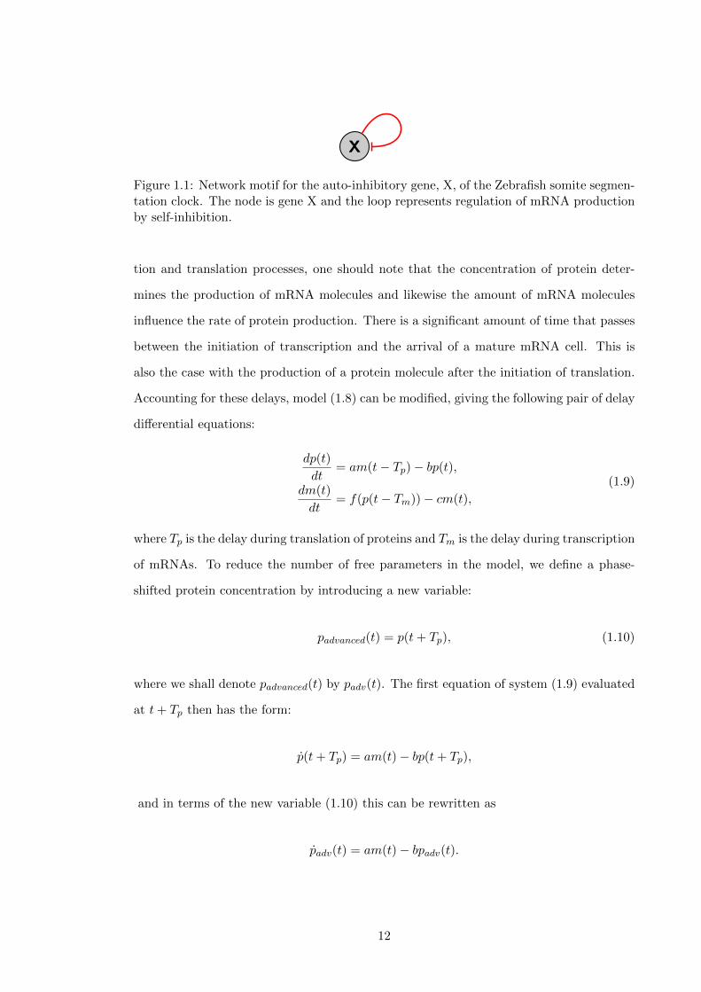
Figure 1.1: Network motif for the auto-inhibitory gene, X, of the Zebrafish somite segmen-tation clock. The node is gene X and the loop represents regulation of mRNA productionby self-inhibition.
tion and translation processes, one should note that the concentration of protein deter-
mines the production of mRNA molecules and likewise the amount of mRNA molecules
influence the rate of protein production. There is a significant amount of time that passes
between the initiation of transcription and the arrival of a mature mRNA cell. This is
also the case with the production of a protein molecule after the initiation of translation.
Accounting for these delays, model (1.8) can be modified, giving the following pair of delay
differential equations:
dp(t)
dt= am(t− Tp)− bp(t),
dm(t)
dt= f(p(t− Tm))− cm(t),
(1.9)
where Tp is the delay during translation of proteins and Tm is the delay during transcription
of mRNAs. To reduce the number of free parameters in the model, we define a phase-
shifted protein concentration by introducing a new variable:
padvanced(t) = p(t+ Tp), (1.10)
where we shall denote padvanced(t) by padv(t). The first equation of system (1.9) evaluated
at t+ Tp then has the form:
p(t+ Tp) = am(t)− bp(t+ Tp),
and in terms of the new variable (1.10) this can be rewritten as
padv(t) = am(t)− bpadv(t).
12

The second equation of system (1.9) transforms into
m(t) = f(padv(t− Tm − Tp))− cm(t).
Thus, omitting the ‘adv’, system (1.9) takes the form:
dp(t)
dt= am(t)− bp(t),
dm(t)
dt= f(p(t− τ))− cm(t),
(1.11)
where τ = Tm + Tp is the new combined time delay [92].
Before continuing with any analysis of system (1.11) we first must establish that the
solutions are nonnegative for all time to ensure their biological feasibility. The initial
conditions for model (1.11) are given by:
p(s) = φ1(s), s ∈ [−τ, 0],
m(s) = φ2(s), s ∈ [−τ, 0],
(1.12)
where φi(s) ∈ C([−τ, 0],R) with φi(s) ≥ 0 (−τ ≤ s ≤ 0, i = 1, 2). Here, C([−τ, 0],R) is
the Banach space of continuous mappings of the interval [−τ, 0] into R. It is also assumed
that m(0) > 0, as this ensures that at least some amount of proteins will be produced.
We now prove that the solution (p(t),m(t)) of DDE (1.11) with the initial condition
(1.12) is positive for all t > 0. This result can be proved by contradiction, following the
methodology used in [93]. We begin by showing that m(t) ≥ 0 for all t > 0. Let t1 > 0
be the first time when p(t1)m(t1) = 0; assuming that m(t1) = 0 implies p(t) ≥ 0 for all
t ∈ [0; t1], and since t1 is the first time when m(t1) = 0, this also means dm(t1)/dt ≤ 0,
that is, the function m(t) is decreasing at t = t1. However, evaluating the second equation
of the system (1.11) at t = t1 yields
dm(t1)
dt=
k
1 + p(t− τ)2/p20
> 0,
which gives a contradiction. Since m(0) > 0, this implies m(t) > 0 for all t > 0. Now that
the positivity of m(t) has been established, let t2 > 0 be the first time when p(t2) = 0.
For this to happen, one must have dp(t2)/dt ≤ 0, that is, the function p(t) should be
13

decreasing at t = t2. At the same time, evaluating the first equation of the system (1.11)
at t = t2 yields
dp(t2)
dt= am(t2) > 0,
which gives a contradiction, therefore, pb(t) > 0 for all t > 0. Hence, solutions p(t) and
m(t) of the model (1.11) are positive for all t > 0.
The steady states p and m of system (1.11) can be found as the roots of the following
system of algebraic equations:
am− bp = 0,
k
1 + p2/p20
− cm = 0.(1.13)
From the first equation of (1.13) we find that m =b
ap. Substituting this into the second
equation of (1.13) leads to the following polynomial equation for p:
p3 + p20p−
akp20
bc= 0,
where a, b, c, p0, k > 0. Replacing p with u− p203u , some algebraic manipulation yields
u6 − akp20
bcu3 − p6
0
27= 0.
This can be easily solved for u3 as
u3 =akp2
0
2bc± 1
2
√a2k2p4
0
b2c2+
4p60
27.
There are six solutions for u, namely
u1,2,3 =3
√akp2
0
2bc+
1
2
√a2k2p4
0
b2c2+
4p60
27.e
2Kπ3i, K = 0, 1, 2,
u4,5,6 =3
√akp2
0
2bc− 1
2
√a2k2p4
0
b2c2+
4p60
27.eπ+2Kπ
3i, K = 0, 1, 2.
(1.14)
A positive real steady state is required in order for it to be biologically relevant, so we
14

only need to look at u1 in (1.14) (where K = 0):
u =3
√akp2
0
2bc+
1
2
√a2k2p4
0
b2c2+
4p60
27. (1.15)
Substituting (1.15) back into p = u − p203u , we are able to express the steady states p and
m of system (1.11) as follows:
p =
(F2 + 1
2
√F 2 +
4p6027
)2/3
− p203(
F2 + 1
2
√F 2 +
4p6027
)1/3, m =
ba
[(F2 + 1
2
√F 2 +
4p6027
)2/3
− p203
](F2 + 1
2
√F 2 +
4p6027
)1/3,
where F =akp20bc .
The equation for eigenvalues λ of the linearisation near the steady state (p, m) of
system (1.11) has the form
λ2 + (b+ c)λ+ bc+ γe−λτ = 0, (1.16)
where
γ =2akp/p2
0
(1 + (p2/p20))2
> 0.
In the limit τ = 0, (1.16) reduces to the quadratic equation:
λ2 + (b+ c)λ+ bc+ γ = 0,
whose roots always have negative real parts since b > 0, c > 0, and γ > 0. This means
that the steady state (p, m) is stable for any choice of parameters. Then to investigate if
there is a point at which the steady state loses stability for τ > 0, we notice that λ = 0
is not a valid solution to the characteristic equation (1.16). Thus, the only way in which
the steady state (p, m) may lose stability is when a pair of complex conjugate roots of
(1.16) cross the imaginary axis. We can investigate this by looking for solutions of the
characteristic equation (1.16) in the form λ = iω for some real ω > 0. Substituting this
15

Figure 1.2: Stability boundary of the steady state (p, m) of system (1.11). The steadystate is stable below the surface in (a) and to the left of the boundary curves shown in(b). Parameter values are c = 0.23, k = 33, and p0 = 40.
into equation (1.16) and separating into real and imaginary parts gives
γ cos(ωτ) = ω2 − bc,
γ sin(ωτ) = (b+ c)ω.
(1.17)
Squaring and adding these two equations together produces the following equation for
z = ω2:
h(z) = z2 + (b2 + c2)z + b2c2 − γ2 = 0,
which can be solved to give the critical frequency:
ω20 =
1
2
[−(b2 + c2) +
√(b2 − c2)2 + 4γ2
]. (1.18)
It should be noted that ω20 will only give real values provided bc < γ. This means that for
the values of parameters such that bc ≥ γ, the steady state (p, m) is stable for all values
of the time delay τ . Note that,
dh(z)
dz= 2z + b2 + c2 > 0, for any z ≥ 0.
16
0 100 200 300 400time t
0
200
400
600
(a)
p(t)m(t)
0 100 200 300 400time t
0
200
400
600
800(b)
p(t)m(t)
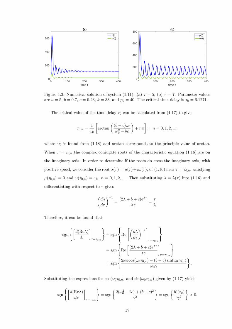
Figure 1.3: Numerical solution of system (1.11): (a) τ = 5; (b) τ = 7. Parameter valuesare a = 5, b = 0.7, c = 0.23, k = 33, and p0 = 40. The critical time delay is τ0 = 6.1271.
The critical value of the time delay τ0 can be calculated from (1.17) to give
τ0,n =1
ω0
[arctan
((b+ c)ω0
ω20 − bc
)+ nπ
], n = 0, 1, 2, ...,
where ω0 is found from (1.18) and arctan corresponds to the principle value of arctan.
When τ = τ0,n the complex conjugate roots of the characteristic equation (1.16) are on
the imaginary axis. In order to determine if the roots do cross the imaginary axis, with
positive speed, we consider the root λ(τ) = µ(τ)+ iω(τ), of (1.16) near τ = τ0,n, satisfying
µ(τ0,n) = 0 and ω(τ0,n) = ω0, n = 0, 1, 2, .... Then substituting λ = λ(τ) into (1.16) and
differentiating with respect to τ gives
(dλ
dτ
)−1
=(2λ+ b+ c)eλτ
λγ− τ
λ.
Therefore, it can be found that
sgn
{[d(Reλ)
dτ
]τ=τ0,n
}= sgn
Re
[(dλ
dτ
)−1]τ=τ0,n
= sgn
{Re
[(2λ+ b+ c)eλτ
λγ
]τ=τ0,n
}
= sgn
{2ω0 cos(ω0τ0,n) + (b+ c) sin(ω0τ0,n)
ω0γ
}.
Substituting the expressions for cos(ω0τ0,n) and sin(ω0τ0,n) given by (1.17) yields
sgn
{[d(Reλ)
dτ
]τ=τ0,n
}= sgn
{2(ω2
0 − bc) + (b+ c)2
γ2
}= sgn
{h′(zk)
γ2
}> 0.
17
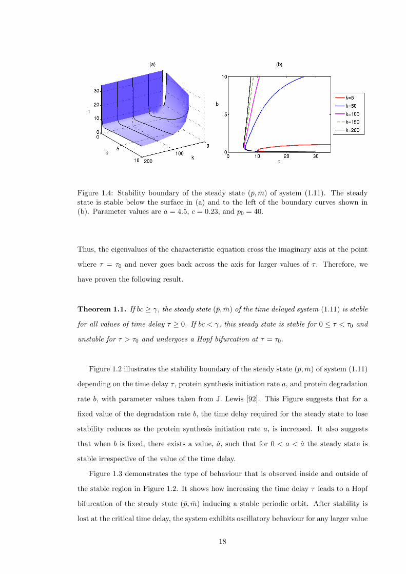
Figure 1.4: Stability boundary of the steady state (p, m) of system (1.11). The steadystate is stable below the surface in (a) and to the left of the boundary curves shown in(b). Parameter values are a = 4.5, c = 0.23, and p0 = 40.
Thus, the eigenvalues of the characteristic equation cross the imaginary axis at the point
where τ = τ0 and never goes back across the axis for larger values of τ . Therefore, we
have proven the following result.
Theorem 1.1. If bc ≥ γ, the steady state (p, m) of the time delayed system (1.11) is stable
for all values of time delay τ ≥ 0. If bc < γ, this steady state is stable for 0 ≤ τ < τ0 and
unstable for τ > τ0 and undergoes a Hopf bifurcation at τ = τ0.
Figure 1.2 illustrates the stability boundary of the steady state (p, m) of system (1.11)
depending on the time delay τ , protein synthesis initiation rate a, and protein degradation
rate b, with parameter values taken from J. Lewis [92]. This Figure suggests that for a
fixed value of the degradation rate b, the time delay required for the steady state to lose
stability reduces as the protein synthesis initiation rate a, is increased. It also suggests
that when b is fixed, there exists a value, a, such that for 0 < a < a the steady state is
stable irrespective of the value of the time delay.
Figure 1.3 demonstrates the type of behaviour that is observed inside and outside of
the stable region in Figure 1.2. It shows how increasing the time delay τ leads to a Hopf
bifurcation of the steady state (p, m) inducing a stable periodic orbit. After stability is
lost at the critical time delay, the system exhibits oscillatory behaviour for any larger value
18
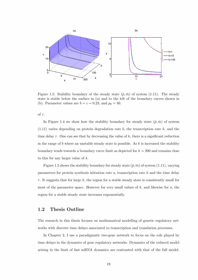
Figure 1.5: Stability boundary of the steady state (p, m) of system (1.11). The steadystate is stable below the surface in (a) and to the left of the boundary curves shown in(b). Parameter values are b = c = 0.23, and p0 = 40.
of τ .
In Figure 1.4 we show how the stability boundary for steady state (p, m) of system
(1.11) varies depending on protein degradation rate b, the transcription rate k, and the
time delay τ . One can see that by decreasing the value of k, there is a significant reduction
in the range of b where an unstable steady state is possible. As k is increased the stability
boundary tends towards a boundary curve limit as depicted for k = 200 and remains close
to this for any larger value of k.
Figure 1.5 shows the stability boundary for steady state (p, m) of system (1.11), varying
parameters for protein synthesis initiation rate a, transcription rate k and the time delay
τ . It suggests that for large k, the region for a stable steady state is consistently small for
most of the parameter space. However for very small values of k, and likewise for a, the
region for a stable steady state increases exponentially.
1.2 Thesis Outline
The research in this thesis focuses on mathematical modelling of genetic regulatory net-
works with discrete time delays associated to transcription and translation processes.
In Chapter 2, I use a paradigmatic two-gene network to focus on the role played by
time delays in the dynamics of gene regulatory networks. Dynamics of the reduced model
arising in the limit of fast mRNA dynamics are contrasted with that of the full model.
19

Stability of steady states are established in terms of the system parameters and analytical
conditions for a Hopf bifurcation are derived for both models. Numerical simulations are
shown to illustrate the dynamical behaviour under different parameter schemes.
Chapter 3 discusses a mathematical model of a genetic regulatory network relevant
for describing the dynamics of transcription factors in the immune system. A three-gene
network is explored to examine the effects of time delays on its dynamics. Conditions for
stability of each steady state are presented where a Hopf bifurcation is possible for one
of the steady states. Numerical simulations help to further understand the results of the
mathematical analysis.
In Chapter 4, I investigate a mathematical model of a genetic regulatory network which
gives rise to oscillation and switch dynamics. A five-gene network is used to discuss the role
of transcriptional and translational time delays on the dynamical behaviour of one protein
in the gene regulatory network by comparing results with earlier literature. Numerical
simulations are used to depict the existence of new behaviour due to the inclusion of time
delays.
Chapter 5 contains a summary of the main results of the thesis and a discussion of
some open problems.
20
Chapter 2
Time-Delayed Models of Gene
Regulatory Networks
Cancer is a complex disease, triggered by multiple mutations in various genes and ex-
acerbated by a number of different behavioural and environmental factors. Some risk
factors associated with possible onset and development of cancer are preventable, such
as, inappropriate diet, physical inactivity, smoking and drinking [94], while other causes
include pathogens (HPV16 and HPV18 are known to cause up to 70% of cervical cancer
cases [95]), as well as genetic pre-disposition. Many studies have focussed on identifying
efficient genetic cancer biomarkers, such as, specific genes and groups of genes associ-
ated with significant number of cases of breast cancer [96], prostate [97] and pancreatic
cancer [98]. Despite this progress, due to significant complexity associated with muta-
tions of various cancer genes, many molecular mechanisms of oncogenesis remain poorly
understood.
Recent advances in microarray and high-throughput sequencing technologies have pro-
vided pathways for measuring the expression of thousands of genes and mapping most
crucial genes and groups of genes controlling different types of cancer.
In order to make progress in understanding the onset and development of cancer, as
well as to develop effective drug targets, it is essential to be able to reconstruct GRNs
pertinent to particular types of cancer from available data. Yeh et al. [99] have used a
K-nearest-neighbours algorithm to identify GRNs correlated with cancer, tumour grade
and stage in prostate cancer. As an alternative approach, Bonnet et al. [100] have utilised
21

LeMoNe (Learning Module Networks) algorithms to derive GRNs from gene and mRNA
expression, as measured in lymphoblastoid cell lines of prostate cancer patients. A rule-
based algorithm has been successfully used to determine GRNs in colon cancer [101],
and similar kinds of networks have been identified from microarray data using neural
fuzzy networks [102]. Madhamshettiwar et al. [103] discuss different approaches to infer
GRNs in ovarian cancer, as well as the potential of using these GRNs to develop optimal
drug targets. Bayesian network techniques have been employed to construct GRNs from
microarray data for breast cancer [104]. In a recent paper, Emmert-Streib et al. [105] have
successfully used a BC3Net inference algorithm to analyse a large-scale breast cancer gene
expression data set and reconstruct the associated GRN.
This chapter is devoted to consideration of the effects of transcriptional and transla-
tional time delays on the dynamics of GRNs. We introduce the time-delayed model of a
two-gene activation-inhibition network together with its quasi-steady state simplification,
and estabilish the well-posedness of both models. We derive analytical conditions for sta-
bility and a Hopf bifurcation in the case of very fast mRNA dynamics, before extending
analysis to the full time-delayed system.
2.1 Time-Delayed Models: Derivation and Positivity
To motivate the analysis of time-delayed effects in gene regulatory dynamics, following
Polynikis et al. [32], we consider an activation-inhibition two-gene GRN consisting of two
genes a and b, which are assumed to have no effect on their own expression; at the same
time, protein Pb is assumed to activate the expression of gene a, while protein Pa inhibits
the expression of gene b. This is one of the fundamental motifs, which has been shown
to be functionally relevant in GRNs [50,106]. Denoting the concentrations of proteins Pa
and Pb as pa and pb, and concentrations of transcribed mRNAs as ra and rb, the following
system of equations can be derived for the dynamics of this GRN [32]:
ra = mah+(pb; θb, nb)− γara,
rb = mbh−(pa; θa, na)− γbrb,
pa = kara − δapa,
pb = kbrb − δbpb,
(2.1)
22

p
0
0.5
1
h+(p; , n)
(a)
n=1n=2n=3n=10
p
0
0.5
1
h-(p; , n)
(b)
n=1n=2n=3n=10
Figure 2.1: Hill functions for activation and inhibition of transcription in system (2.1),varying the Hill coefficient, n. (a) Activation function. (b) Inhibition function.
where mi are the maximum transcription rates, ki are the translation rates, γi are the
mRNA degradation rates, and δi are the protein degradation rates for i = a, b. Equations
(2.1) are called the complete nonlinear model (CNM). To make further analytical progress,
the activation and inhibition functions in the system (2.1) can be written as the following
Hill functions:
h+(pi; θi, ni) =pnii
pnii + θnii,
h−(pi; θi, ni) = 1− h+(pi; θi, ni) =θnii
pnii + θnii, i = a, b,
where θa and θb are known as activation and inhibition coefficients, and the integer pa-
rameters na and nb, known as Hill coefficients, determine the steepness of Hill curves [1].
The parameters θa and θb give the values of protein concentrations pa and pb, at which the
corresponding Hill function achieves half of its maximum value. Depending on the values
of transcription rates, this would then lead to a significant increase in the respective mR-
NAs regulated by these proteins [3, 32]. A qualitative illustration of the activation and
inhibition Hill functions is given in Figure 2.1.
Due to the fact that the dynamics of mRNA is normally much faster than that of
related proteins, one can use a quasi-steady state assumption to simplify the CNM (2.1)
by reducing the number of equations. Effectively, this means assuming that mRNAs have
already reached their steady-state concentrations, i.e. taking ri ≈ 0, i = a, b in the
CNM (2.1), and then focusing on the dynamics of proteins only, as given by the following
23
simplified nonlinear model (SNM):
pa = k′ah+(pb; θb, nb)− δapa,
pb = k′bh−(pa; θa, na)− δbpb,
where
k′a =makaγa
, k′b =mbkbγb
. (2.2)
Polynikis et al. [32] have shown that while the CNM exhibits Hopf bifurcation of a pos-
itive equilibrium, leading to persistent oscillations, in the case of the SNM model this
behaviour can disappear. They have also demonstrated an important role played by the
Hill coefficients, as well as the separation of timescales between mRNA and proteins, with
a larger scale separation favouring a stable equilibrium rather than oscillatory behaviour.
While the transcription and translation may be faster than characteristic times as-
sociated with significant changes in protein concentrations (of the order of 5 minutes for
transcription + translation and 1 hour for a 50% change in the concentration of translated
protein for E. coli. [1]), these are, in fact, multi-step processes consisting of thousands of
consecutive chemical reactions. Hence, the duration of transcription and translation is
non-negligible when considered in the context of GRN dynamics [72, 84], and has to be
correctly accounted for in mathematical models. To analyse the effects of transcriptional
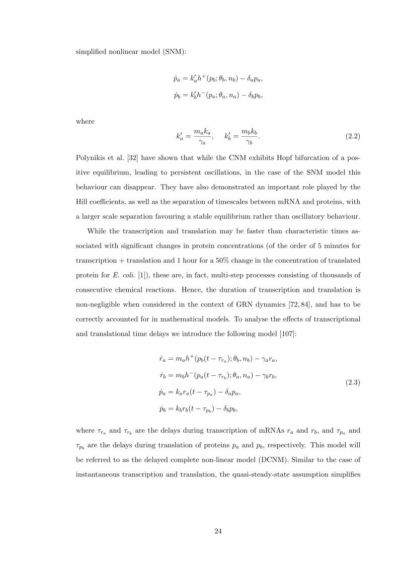
and translational time delays we introduce the following model [107]:
ra = mah+(pb(t− τra); θb, nb)− γara,
rb = mbh−(pa(t− τrb); θa, na)− γbrb,
pa = kara(t− τpa)− δapa,
pb = kbrb(t− τpb)− δbpb,
(2.3)
where τra and τrb are the delays during transcription of mRNAs ra and rb, and τpa and
τpb are the delays during translation of proteins pa and pb, respectively. This model will
be referred to as the delayed complete non-linear model (DCNM). Similar to the case of
instantaneous transcription and translation, the quasi-steady-state assumption simplifies
24
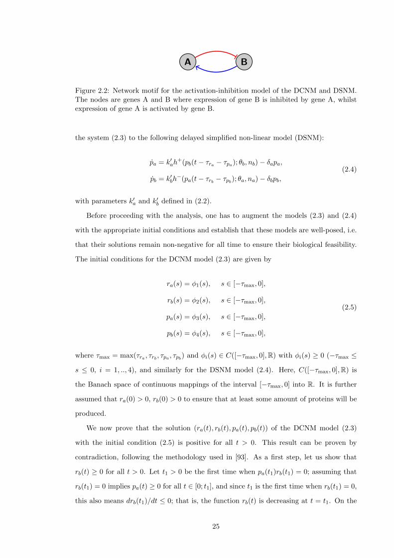
A B
Figure 2.2: Network motif for the activation-inhibition model of the DCNM and DSNM.The nodes are genes A and B where expression of gene B is inhibited by gene A, whilstexpression of gene A is activated by gene B.
the system (2.3) to the following delayed simplified non-linear model (DSNM):
pa = k′ah+(pb(t− τra − τpa); θb, nb)− δapa,
pb = k′bh−(pa(t− τrb − τpb); θa, na)− δbpb,
(2.4)
with parameters k′a and k′b defined in (2.2).
Before proceeding with the analysis, one has to augment the models (2.3) and (2.4)
with the appropriate initial conditions and establish that these models are well-posed, i.e.
that their solutions remain non-negative for all time to ensure their biological feasibility.
The initial conditions for the DCNM model (2.3) are given by
ra(s) = φ1(s), s ∈ [−τmax, 0],
rb(s) = φ2(s), s ∈ [−τmax, 0],
pa(s) = φ3(s), s ∈ [−τmax, 0],
pb(s) = φ4(s), s ∈ [−τmax, 0],
(2.5)
where τmax = max(τra , τrb , τpa , τpb) and φi(s) ∈ C([−τmax, 0],R) with φi(s) ≥ 0 (−τmax ≤
s ≤ 0, i = 1, .., 4), and similarly for the DSNM model (2.4). Here, C([−τmax, 0],R) is
the Banach space of continuous mappings of the interval [−τmax, 0] into R. It is further
assumed that ra(0) > 0, rb(0) > 0 to ensure that at least some amount of proteins will be
produced.
We now prove that the solution (ra(t), rb(t), pa(t), pb(t)) of the DCNM model (2.3)
with the initial condition (2.5) is positive for all t > 0. This result can be proven by
contradiction, following the methodology used in [93]. As a first step, let us show that
rb(t) ≥ 0 for all t > 0. Let t1 > 0 be the first time when pa(t1)rb(t1) = 0; assuming that
rb(t1) = 0 implies pa(t) ≥ 0 for all t ∈ [0; t1], and since t1 is the first time when rb(t1) = 0,
this also means drb(t1)/dt ≤ 0; that is, the function rb(t) is decreasing at t = t1. On the
25

other hand, evaluating the second equation of the system (2.3) at t = t1 yields
drb(t1)
dt=
mbθnaa
pa(t1 − τrb)na + θnaa> 0,
which gives a contradiction. Since rb(0) > 0, this implies rb(t) > 0 for all t > 0. Now that
the positivity of rb(t) has been established, let t2 > 0 be the first time when pb(t2) = 0. In
order for this to happen, one must have dpb(t2)/dt ≤ 0; that is, the function pb(t) should
be decreasing at t = t2. At the same time, evaluating the last equation of the system (2.3)
at t = t2 yields
dpb(t2)
dt= kbrb(t2 − τpb) > 0,
which gives a contradiction and, therefore, pb(t) > 0 for all t > 0. In a similar manner,
the positivity of pb(t) implies the positivity of ra(t), which in turn implies the positivity
of pa(t). Hence, all solutions ra(t), rb(t), pa(t) and pb(t) of the DCNM model (2.3) are
positive for all t > 0. The same approach can be employed to show positivity of solutions
of DSNM model (2.4).
Steady states (ra, rb, pa, pb) of the DCNM model can be found as roots of the following
system of algebraic equations:
mah+(pb; θb, nb)− γara = 0,
mbh−(pa; θa, na)− γbrb = 0,
kara − δapa = 0,
kbrb − δbpb = 0.
This gives
ra =δakapa, rb =
δbkbpb, pb =
φbθnaa
θnaa + pnaa,
where pa satisfies the polynomial equation
θnbb
nb∑k=0
(nbk
)pna(nb−k)+1a θnaka + (pa − φa)(φbθnaa )nb = 0, (2.6)
and we used the notation
φa =makaγaδa
, φb =mbkbγbδb
.
26
Even for realistically small values of Hill coefficients, such as n = 2, 3 [108] or n = 4-
8 [109], (2.6) is too complicated to allow one to analytically find closed form expressions
for pa and other state variables. Despite not having explicit formulae for possible steady
states (ra, rb, pa, pb), one can still perform the analysis of stability in terms of system
parameters, and such results would be valid for the values of steady state variables that
can be accurately and efficiently determined through numerical solution of the polynomial
equation (2.6).
2.2 Analysis of the Delayed Simplified Nonlinear Model
(DSNM)
In order to gain some first insights into the role of transcriptional and translational delays
on the dynamics of GRN, we focus on the behaviour of the delayed simplified nonlinear
model (DSNM) (2.4). To reduce the number of free parameters in the model, we introduce
the new variables:
pa(t) = pa(t), pb(t) = pb(t− τra − τpa), (2.7)
which transform the first equation of system (2.4) into
pa = k′ah+(pb(t− τra − τpa); θb, nb)− δapa ⇐⇒ ˙pa(t) = k′ah
+(pb(t); θb, nb)− δapa(t).
The second equation of system (2.4) evaluated at t− τra − τpa has the form
pb(t− τra − τpa) = k′bh−(pa(t− τra − τpa − τrb − τpb); θa, na)− δbpb(t− τra − τpa),
and in terms of the new variables (2.7) this can be rewritten as
˙pb(t) = k′bh−(pa(t− τra − τpa − τrb − τpb); θa, na)− δbpb(t).
Thus, system (2.4) takes form
˙pa(t) = k′ah+(pb(t); θb, nb)− δapa(t),
˙pb(t) = k′bh−(pa(t− τ); θa, na)− δbpb(t),
(2.8)
27

where
τ = τra + τpa + τrb + τpb
is the new combined time delay. The equation for eigenvalues λ of the linearisation near
a steady state (pa, pb) of system (2.8) has the form
(λ+ δa)(λ+ δb) +DDSNMe−λτ = 0, (2.9)
where
DDSNM = k′ak′bnanb
θnaa θnbb p(na−1)a p
(nb−1)b
(θnaa + pnaa )2(θnbb + pnbb )2= nanbδaδb
pnaaθnaa + pnaa
θnbbθnbb + pnbb
.
In the limit τ = 0, this equation reduces to the quadratic equation [32]:
λ2 + (δa + δb)λ+ δaδb +DDSNM = 0,
whose roots always have negative real parts, since δa > 0, δb > 0 and DDSNM > 0. This
implies that, for τ = 0, the steady state (pa, pb) is stable for any values of parameters. To
investigate whether this steady state can lose stability for τ > 0, one can note that λ = 0
is not a solution of the characteristic equation (2.9). Hence, the only possible way that the
steady state (pa, pb) can lose its stability is when a pair of complex conjugate eigenvalues
crosses the imaginary axis. In the light of this observation, one can look for eigenvalues
of (2.9) in form λ = iω for some real ω > 0. Substituting this into (2.9) and separating
into real and imaginary parts gives
ω2 − δaδb = DDSNM cos(ωτ),
(δa + δb)ω = DDSNM sin(ωτ).
(2.10)
Squaring and adding these two equations yields the following equation for z = ω2:
h(z) = z2 + (δ2a + δ2
b )z + δ2aδ
2b −D2
DSNM = 0,
which can be solved to give the critical frequency as
ω20 =
1
2
[−(δ2
a + δ2b ) +
√(δ2a + δ2
b )2 − 4(δ2
aδ2b −D2
DSNM)
]. (2.11)
28

One should note that ω20 will only admit positive real values, provided δaδb < DDSNM,
which implies that, for δaδb ≥ DDSNM, the steady state (pa, pb) is stable for all values of
the time delay τ . Note that
dh(z)
dz= 2z + δ2
a + δ2b > 0 for any z ≥ 0.
The critical value of the time delay τ can be found from (2.10), which gives
τ0,n =1
ω0
[arctan
((δa + δb)ω0
ω20 − δaδb
)+ nπ
], n = 0, 1, 2, ...,
where ω0 is determined by (2.11), and arctan corresponds to the principal value of arctan.
When τ = τ0,n, the characteristic equation (2.9) has a pair of purely imaginary roots.
To determine whether or not these roots do indeed cross the imaginary axis, we consider
λ(τ) = µ(τ) + iω(τ) as a root of (2.9) near τ = τ0,n, satisfying µ(τ0,n) = 0, ω(τ0,n) = ω0,
and j = 0, 1, 2, .... Substituting λ = λ(τ) into (2.9) and differentiating with respect to τ
yields (dλ
dτ
)−1
=(2λ+ δa + δb)e
λτ
λDDSNM− τ
λ.
From this equation, one can find
sgn
{[d(Reλ)
dτ
]τ=τ0,n
}= sgn
Re
[(dλ
dτ
)−1]τ=τ0,n
= sgn
{Re
[(2λ+ δa + δb)e
λτ
λDDSNM
]τ=τ0,n
}
= sgn
{2ω0 cos(ω0τ0,n) + (δa + δb) sin(ω0τ0,n)
ω0DDSNM
}.
Substituting the expressions for cos(ω0τ0,n) and sin(ω0τ0,n) from system (2.10) gives
sgn
{[d(Reλ)
dτ
]τ=τ0,n
}= sgn
{2(ω2
0 − δaδb) + (δa + δb)2
D2DSNM
}= sgn
{h′(ω2
0)
D2DSNM
}> 0.
Hence, the eigenvalues of the characteristic equation cross the imaginary axis at τ = τ0
(here, τ0 = τ0,0) and never cross back for higher values of τ . Thus, we have proved the
following result.
29

Figure 2.3: Stability boundary of the steady state (pa, pb) of DSNM system (2.8). Thesteady state is stable below the surface in (a) and to the left of the boundary curvesshown in (b). Parameter values are ma = mb = 2.35, θa = θb = 0.21, na = nb = 3, andka = kb = γa = γb = 1.
Theorem 2.1. If δaδb ≥ DDSNM, the steady state (pa, pb) of DSNM system (2.8) is stable
for all values of the time delay τ ≥ 0. If δaδb < DDSNM, this steady state is stable for
0 ≤ τ < τ0 and unstable for τ > τ0 and undergoes a Hopf bifurcation at τ = τ0.
Figure 2.3 illustrates the stability boundary of the steady state (pa, pb) of the DSNM
system (2.8) depending on the time delay τ and the protein degradation rates δa and δb,
with the parameter values taken from Polynikis et al. [32]. This Figure suggests that, for
any fixed value of one of such rates, there is only a limited range of positive values of
the other degradation rate, for which, at a given time delay τ , the positive equilibrium is
unstable. For sufficiently high values of δa and δb, this steady state is stable regardless of
the value of the time delay τ , confirming the result proved in Theorem 2.1.
In Figure 2.4 we show how the stability boundary varies depending on the parameters
θa and θb, and the time delay τ . One observes that, for sufficiently high values of θb, the
range of possible values of θa for which the steady state is unstable is significantly reduced,
thus making the system more prone to support a stable positive equilibrium rather than
exhibit oscillations. At the Hopf bifurcation, the associated critical value of the time delay
τ monotonically increases with the parameter θa. At the same time, there is a minimum
30

Figure 2.4: Stability boundary of the steady state (pa, pb) of DSNM system (2.8). Thesteady state is stable below the surface in (a) and (c) and to the left of the boundarycurves shown in (b) and (d). Parameter values are ma = mb = 2.35, na = nb = 3, andka = kb = δa = δb = γa = γb = 1.
value of the time delay τ , such that for τ smaller than this value the steady state (pa, pb)
is stable for any value of θa.
In a similar way, the effects of the transcription rates ma and mb are illustrated in Fig-
ure 2.5, which shows that the critical transcription rate of the inhibitor ma increases with
decreasing τ , and, similar to Figure 2.4, below certain value of τ , the steady state (pa, pb)
is stable for any value of ma. Qualitatively similar dependence is observed between the
critical value of τ and the transcription rate mb, though this dependence is not completely
monotonic.
Figure 2.6 demonstrates how increasing the overall time delay τ results in a Hopf
bifurcation of the steady state (pa, pb) and the emergence of a stable periodic orbit. The
31

Figure 2.5: Stability boundary of the steady state (pa, pb) of DSNM system (2.8). Thesteady state is stable below the surface in (a), and to the left of the boundary curvesshown in (b). Parameter values are θa = θb = 0.21, na = nb = 3, and ka = kb = δa = δb =γa = γb = 1.
0 10 20 300
0.5
1
1.5
2
time t
(a)
pa(t)
pb(t)
0 10 20 30 400
1
2
time t
(b)
pa(t)
pb(t)
Figure 2.6: Numerical solution of DSNM system (2.8): (a) τ = 0.5; (b) τ = 2. Parametervalues are ma = mb = 2.35, θa = θb = 1, na = nb = 3, and ka = kb = δa = δb = γa = γb =1. The critical time delay is τ0 = 0.9762.
shift between individual time series for pa and pb can be interpreted in the same way as in
predator-prey or activator-inhibitor systems [110]. In accordance with Theorem 2.1, once
the stability of the steady state (pa, pb) is lost, it can never be regained for higher values
of τ , so the system will be exhibiting oscillatory behaviour. This result highlights the
significance of correct mathematical representation of the transcription and translation
processes, since inclusion of transcriptional and translational delays can lead to sustained
periodic oscillations even in the simplified model, where such oscillations were impossible
when the time delays were neglected.
32

2.3 Analysis of the Delayed Complete Nonlinear Model
(DCNM)
Linearisation of the full nonlinear DCNM model (2.3) near the steady state (ra, rb, pa, pb)
results in the following characteristic equation:
(λ+ γa)(λ+ γb)(λ+ δa)(λ+ δb) +DDCNMe−λτ = 0, (2.12)
where
DDCNM = mambkakbθnaa θnbb
nanbp(na−1)a p
(nb−1)b
(θnaa + pnaa )2(θnbb + pnbb )2= nanbδaδbγaγb
pnaaθnaa + pnaa
θnbbθnbb + pnbb
,
and
τ = τra + τrb + τpa + τpb .
It immediately follows from the form of the characteristic equation (2.12) that stability of
the steady state (ra, rb, pa, pb) is determined not by individual transcriptional and transla-
tional delays but rather by their overall combined duration. In the case τra = τrb = τpa =
τpb = 0, the characteristic equation of the DCNM model reduces to the one analysed in
Polynikis et al. [32].
The characteristic equation (2.12) can be recast in the form
λ4 +Aλ3 +Bλ2 + Cλ+ (D +DDCNMe−λτ ) = 0, (2.13)
where
A = γa + γb + δa + δb,
B = γaγb + γaδa + γaδb + γbδa + γbδb + δaδb,
C = γaγbδa + γaγbδb + γaδaδb + γbδaδb,
D = γaγbδaδb.
(2.14)
At τ = 0, (2.13) reduces to a quartic
λ4 +Aλ3 +Bλ2 + Cλ+ (D +DDCNM) = 0. (2.15)
33

By the Routh-Hurwitz criterion [110], the necessary and sufficient conditions for all roots
of (2.15) to have negative real parts are given by
∆1 = A > 0,
∆2 = AB − C > 0,
∆3 = ABC −A2(D +DDCNM) > 0,
∆4 = (D +DDCNM)(ABC −A2(D +DDCNM)− C2) = (D +DDCNM)(∆3 − C2) > 0.
From the fact that all system parameters are positive and using the definitions of A, B,
and C in (2.14), it follows that ∆1 > 0 and ∆2 > 0 for any values of the parameters. Since
D +DDCNM > 0, it is sufficient to require ∆4 > 0 to ensure that condition ∆3 > 0 is also
satisfied. This leads to the following result.
Lemma 2.1. Let τ = 0. The steady state (ra, rb, pa, pb) of the system (2.3) is stable
whenever the condition ABC −A2(D +DDCNM)− C2 > 0 holds.
From now on, we will assume that the condition in Lemma 2.1 holds and analyse
whether stability can be lost as τ increases. Since both D and DDCNM are positive,
this means that λ = 0 is not a root of the characteristic equation (2.13), so once again
the stability can only be lost through a possible Hopf bifurcation. To investigate this
possibility, we look for solutions of (2.13) in the form λ = iω for some real ω > 0.
Substituting this into (2.13) and separating into the real and imaginary parts gives
ω4 −Bω2 +D = −DDCNM cos(ωτ),
−Aω3 + Cω = DDCNM sin(ωτ).
(2.16)
Squaring and adding these equations yields a quartic equation as follows:
g(z) = z4 + az3 + bz2 + cz + d = 0, (2.17)
34
where z = ω2 and
a = A2 − 2B,
b = B2 + 2D − 2AC,
c = C2 − 2BD,
d = D2 −D2DCNM.
Without loss of generality, suppose that (2.17) has four positive real roots, denoted by
z1, z2, z3, z4, respectively, which would give four possible values of ω:
ω1 =√z1, ω2 =
√z2, ω3 =
√z3, ω4 =
√z4.
Dividing the two equations in (2.16) gives
tan(ωkτk) =Aω3
k − Cωkω4k −Bω2
k +D=⇒ τk,j =
1
ωk
[arctan
(Aω3
k − Cωkω4k −Bω2
k +D
)+ jπ
],
k = 1, .., 4, j = 0, 1, 2, ....
Define
τ0 = min1≤k≤4
{τk,0}, ω0 = ωk0 , k0 ∈ {1, 2, 3, 4},
and then τ0 is the first value of τ > 0 such that the characteristic equation (2.13) has a
pair of purely imaginary roots. We have the following result.
Theorem 2.2. Suppose the conditions of Lemma 2.1 hold and g′(z0) > 0, where g(z)
is defined in (2.17). Then the steady state (ra, rb, pa, pb) of system (2.3) is stable for
0 ≤ τ < τ0 and unstable for τ > τ0 and undergoes a Hopf bifurcation at τ = τ0.
Proof. The conclusion of Lemma 2.1 ensures the steady state (ra, rb, pa, pb) of system (2.3)
is stable at τ = 0, and the fact that the roots of the characteristic equation (2.13) depend
continuously on τ implies that the steady state (ra, rb, pa, pb) is also stable for sufficiently
small positive values of τ . Since τ0 is the first positive τ , for which the eigenvalues lie on the
imaginary axis, in order to verify whether or not the steady state actually loses stability
35

at τ = τ0, one has to compute the sign of dRe(λ)/dτ |τ=τ0 . Let λ(τ) = µ(τ) + iω(τ) be the
root of the characteristic equation (2.13) near τ = τ0, satisfying µ(τ0) = 0 and ω(τ0) = ω0.
Substituting λ = λ(τ) into (2.13) and differentiating both sides with respect to τ gives
(dλ
dτ
)−1
=(4λ3 + 3Aλ2 + 2Bλ+ C)eλτ
λDDCNM− τ
λ.
This implies, with λ(τ0) = iω0,
sgn
{[d(Reλ)
dτ
]τ=τ0
}= sgn
{Re
[(dλ
dτ
)−1]τ=τ0
}
= sgn
{Re
[(4λ3 + 3Aλ2 + 2Bλ+ C)eλτ
λDDCNM
]τ=τ0
}
= sgn
{(2Bω0 − 4ω3
0) cos(ω0τ0) + (C − 3Aω20) sin(ω0τ0)
ω0DDCNM
}.
Using the expressions for cos(ω0τ0) and sin(ω0τ0) from (2.16) gives
sgn
{[d(Reλ)
dτ
]τ=τ0
}= sgn
{4ω6
0 + (3A2 − 6B)ω40 + (2B2 + 4D − 4AC)ω2
0 + C2 − 2BD
D2DCNM
}= sgn
{g′(ω2
0)
D2DCNM
}> 0,
which means that at τ = τ0 a pair of complex conjugate eigenvalues of the characteristic
equation (2.13) crosses the imaginary axis with a positive speed. This implies that the
steady state (ra, rb, pa, pb) of system (2.3) does lose its stability at τ = τ0. �
Figure 2.7 shows the stability boundary of the steady state (ra, rb, pa, pb) of system
(2.3) depending on the transcription rates ma and mb and the total time delay τ . In a
manner similar to that for the simplified model, the critical value of the transcription rate
ma at the Hopf bifurcation reduces with increasing τ . However, a major difference from
the DSNM model, as shown in Figure 2.5, is that now the Hopf bifurcation can take place
even at τ = 0, as the DCNM system is able to support sustained oscillations [32]. In
Figure 2.8 we illustrate the transition from a stable steady state (ra, rb, pa, pb) to a stable
periodic solution around this steady state as the time delay passes through the critical
value of τ = τ0.
36

Figure 2.7: Stability boundary of the steady state (ra, rb, pa, pb) of DCNM system (2.3).The steady state is stable below the surface in (a), (c), and below the boundary curvesshown in (b), (d). Parameter values: θa = θb = 0.21, na = nb = 3 and ka = kb = δa =δb = γa = γb = 1.
2.4 Discussion
In this chapter we have discussed mathematical models for the analysis of GRNs and
focussed on the role played by the transcriptional and translational time delays in the
dynamics of a two-gene activator-inhibitor GRN. By reducing the model to the one with a
single time delay, we have considered possible behaviour in the quasi-steady state approx-
imation of very fast mRNA dynamics, which has resulted in a lower-dimensional system
of DDEs. Due to the presence of time delays, even this simplified model is able to exhibit
loss of stability of the positive equilibrium through a Hopf bifurcation and a subsequent
emergence of sustained periodic oscillations, which was not possible in the absence of the
37

0 50 100 150 200
0.1
0.2
0.3
0.4(a)
time t
ra(t)
rb(t)
pa(t)
pb(t)
0 20 40 60 800
0.2
0.4
(b)
time t
ra(t)
rb(t)
pa(t)
pb(t)
Figure 2.8: Numerical solution of DCNM system (2.3): (a) τ = 0.25; (b) τ = 2. Parametervalues: ma = 0.6, mb = 0.3, θa = θb = 0.21, na = nb = 3, and ka = kb = δa = δb = γa =γb = 1. The critical time delay is τ0 = 0.5314.
time delays, as discussed in Polynikis et al. [32]. We have found analytically the boundary
of the Hopf bifurcation depending on the total time delay and other system parameters
and illustrated different types of behaviour by direct numerical simulations. Our results
suggest that once the positive steady state loses its stability, it can never regain it for
higher values of the time delay.
We have also studied the stability of a positive steady state in the full system and
showed that this steady state can also undergo a Hopf bifurcation depending on the time
delay and system parameters. Our analysis extends an earlier result of Polynikis et al. [32]
by showing how the critical values of the parameters at the Hopf boundary change when
the time delay increases from zero. Numerical simulations have illustrated the transition
from a stable positive steady state to a stable periodic solution as the time delay exceeds
its critical value.
Besides providing insights into the dynamics of GRNs, there are several practical ways
in which models similar to the one described in this chapter are helpful for monitoring
and treatment of cancer. GRN models based on differential equations coupled with other
techniques, such as machine learning and Bayesian networks, have proved effective in
identifying specific oncogenes that can be used as biomarkers or drug targets [50,104,111–
114]. Similar kinds of models are useful for modelling cancer cell growth and understanding
interactions between tumour growth and immune response and for analysis of the effects of
38

chemotherapy (or immunotherapy) and drug resistance [50,51,115,116]. The methodology
described in this chapter can be directly used to improve the performance of these models
by elucidating the role of transcriptional and translational time delays in GRN dynamics
and its impact on various aspects of cancer onset and development.
39

Chapter 3
Time-Delayed Model of a Genetic
Regulatory Network in the
Immune System
Recent studies have highlighted the physical applications of GRNs to model cell dynamics
in the immune system [117]. The immune system is a complex system of cells and molecules
that can provide us with a basic defence against pathogenic organisms. Like the nervous
system, the immune system performs pattern recognition tasks, learns, and retains a
memory of the antigens that it has fought. Furthermore, the immune response develops
in time and the description of its time evolution is an interesting problem in dynamical
systems [118].
An area of research in immunology that is of particular interest is the ability to develop
deterministic models for cell fates. Sciammas et al. [119] have used a chemical kinetic
approach based on ordinary differential equations (ODEs) to develop a model for a GRN
that regulates the cell fate dynamics of activated B cells undergoing a germinal centre
(GC) response and then differentiating into plasma cells. The architecture of this GRN
involves the mutual repression of several transcription factors (TFs), namely a TF of the
plasma-cell program, Blimp1, as well as Bcl6 which is essential for GC B cells. In this
network design there exists a TF, IRF4, which activates both genes, and also positive
feedback based on the mutual activation of Blimp1 and IRF4 [117]. The dynamics that
appear as a result of the varied connections between transcription factors provide valuable
40
insight into the behaviour of proteins in the immune system.
Modelling dynamics of T cells have also been extensively studied [120–123]. H. J. van
den Ham et al. developed a simple master regulator for the Th1/Th2 paradigm, which
can be extended to higher dimensions for larger networks and enables the analysis of
other cell types. This general model, however, is mechanistic in characterising binding
of transcription factors but due to its simplicity, allows for the study of larger networks.
A more deterministic approach was carried out by W. C. Lo [123], who modelled the
concentrations of the transcription factors T-Bet (Th1), Gata3 (Th2), and Foxp3 (Treg)
in a cell using ODEs. This meant they were able to account for influences from external
activators, mutual inhibition, and auto-activation which is modelled using Hill functions.
However, mathematical analysis of larger networks using this approach would be very
challenging.
Due to the vast number of connections between transcription factors in the immune
system, the aim is to be able to model complex networks whilst still capturing useful
information about the system dynamics. There have been many different network motifs
explored and analysed to various degrees of complexity [124–127]. T. Hong et al. build
on their previous work by exploring a three and four master regulator symmetric motif,
to describe the interactions between the master transcription factors T-Bet, Gata3, Foxp3
and Rorγt (Th17). It is shown that mathematical analysis and numerical simulation
agree with experimental data. This observation motivates investigation into networks
with multiple nodes, where inhibition and positive feedback loops are present, to model
the dynamics of GRNs in the immune system.
This chapter focuses on the transcriptional and translational delays in a system of three
genes, each of which promotes the growth of its own proteins, and expresses unidirectional
inhibition. We discuss the works of Andrecut et al. [128] and H. El Samad et al. [129] and
derive a delayed model based on the so-called Repressilator. We analyse the model and
derive conditions for the existence of a Hopf bifurcation leading to periodic oscillations,
which could not be present for such a low Hill coefficient in the symmetric Repressilator
model. Numerical simulations are discussed, which give rise to interesting patterns of
stability regions in the parameter space due to the inclusion of multiple time delays. It
is also illustrated that only one of the possible 9 steady states has the potential to lose
stability.
41

3.1 Derivation of the Time-Delayed Model
We take insight from the general model studied by Andrecut et al. [128] for describing
auto-activation and mutual repression between two general proteins, which has equations
given by
dx
dt=
ax
xy + bx+ cy + d− fx,
dy
dt=
ay
xy + by + cx+ d− fy,
(3.1)
where x and y are the two system variables of the generic dynamical system, which can
be taken to describe the concentrations of protein x and protein y. The first term of each
equation in (3.1) describe both auto-activation and mutual inhibition, and the second
terms are degradation for each protein. Note that the growth terms are of the form
(x
θx + x
)(θxy
θxy + y
)=
θxyx
xy + θxyx+ θxy + θxθxy, (3.2)
where the left hand side of the equation consists of two Hill functions with Hill coefficient
n = 1; the first term representing auto-activation of protein x, and the second is repression
of x by protein y.
Here we investigate a three-gene asymmetric model with time delays accounting for
those present in auto-activation and mutual repression processes. The model is given by
the following set of delay differential equations:
dx
dt=
a1x(t− τax)
x(t− τax)z(t− τrx) + b1x(t− τax) + c1z(t− τrx) + d1− f1x,
dy
dt=
a2y(t− τay)y(t− τay)x(t− τry) + b2y(t− τay) + c2x(t− τry) + d2
− f2y,
dz
dt=
a3z(t− τaz)z(t− τaz)y(t− τrz) + b3z(t− τaz) + c3y(t− τrz) + d3
− f3z,
(3.3)
where τax, τay and τaz are the transcriptional delays associated to the auto-activation of
proteins x, y, and z, while τrx, τry, and τrz are the transcriptional delays associated to the
repression of proteins x, y, and z respectively.
42
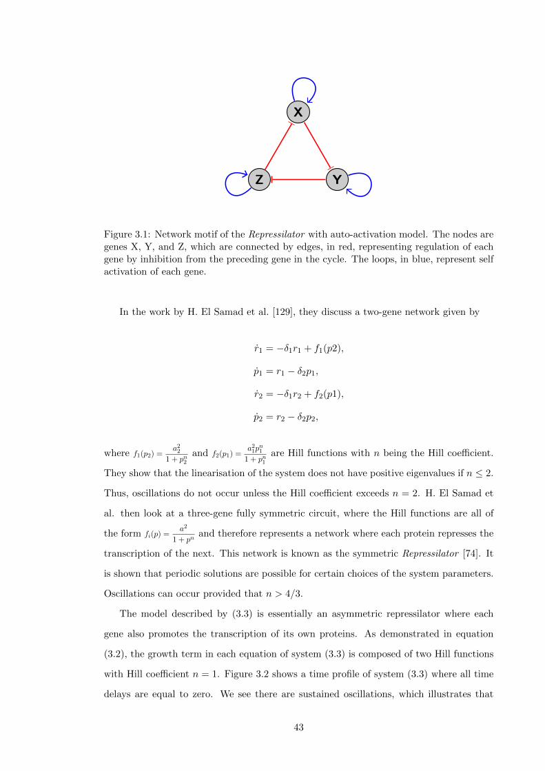
X
YZ
Figure 3.1: Network motif of the Repressilator with auto-activation model. The nodes aregenes X, Y, and Z, which are connected by edges, in red, representing regulation of eachgene by inhibition from the preceding gene in the cycle. The loops, in blue, represent selfactivation of each gene.
In the work by H. El Samad et al. [129], they discuss a two-gene network given by
r1 = −δ1r1 + f1(p2),
p1 = r1 − δ2p1,
r2 = −δ1r2 + f2(p1),
p2 = r2 − δ2p2,
where f1(p2) =a2
2
1 + pn2and f2(p1) =
a21pn1
1 + pn1are Hill functions with n being the Hill coefficient.
They show that the linearisation of the system does not have positive eigenvalues if n ≤ 2.
Thus, oscillations do not occur unless the Hill coefficient exceeds n = 2. H. El Samad et
al. then look at a three-gene fully symmetric circuit, where the Hill functions are all of
the form fi(p) =a2
1 + pnand therefore represents a network where each protein represses the
transcription of the next. This network is known as the symmetric Repressilator [74]. It
is shown that periodic solutions are possible for certain choices of the system parameters.
Oscillations can occur provided that n > 4/3.
The model described by (3.3) is essentially an asymmetric repressilator where each
gene also promotes the transcription of its own proteins. As demonstrated in equation
(3.2), the growth term in each equation of system (3.3) is composed of two Hill functions
with Hill coefficient n = 1. Figure 3.2 shows a time profile of system (3.3) where all time
delays are equal to zero. We see there are sustained oscillations, which illustrates that
43
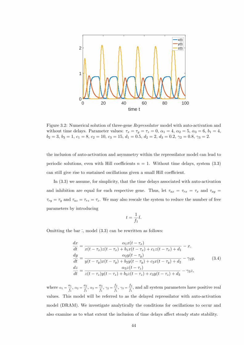
0 20 40 60 80 100time t
0
1
2
x(t)y(t)z(t)
Figure 3.2: Numerical solution of three-gene Repressilator model with auto-activation andwithout time delays. Parameter values: τx = τy = τz = 0, α1 = 4, α2 = 5, α3 = 6, b1 = 4,b2 = 3, b3 = 1, c1 = 8, c2 = 10, c3 = 15, d1 = 0.5, d2 = 2, d3 = 0.2, γ2 = 0.8, γ3 = 2.
the inclusion of auto-activation and asymmetry within the repressilator model can lead to
periodic solutions, even with Hill coefficients n = 1. Without time delays, system (3.3)
can still give rise to sustained oscillations given a small Hill coefficient.
In (3.3) we assume, for simplicity, that the time delays associated with auto-activation
and inhibition are equal for each respective gene. Thus, let τax = τrx = τx and τay =
τry = τy and τaz = τrz = τz. We may also rescale the system to reduce the number of free
parameters by introducing
t =1
f1t.
Omitting the bar ., model (3.3) can be rewritten as follows:
dx
dt=
α1x(t− τx)
x(t− τx)z(t− τx) + b1x(t− τx) + c1z(t− τx) + d1− x,
dy
dt=
α2y(t− τy)y(t− τy)x(t− τy) + b2y(t− τy) + c2x(t− τy) + d2
− γ2y,
dz
dt=
α3z(t− τz)z(t− τz)y(t− τz) + b3z(t− τz) + c3y(t− τz) + d3
− γ3z,
(3.4)
where α1 =a1
f1, α2 =
a2
f1, α3 =
a3
f1, γ2 =
f2
f1, γ3 =
f3
f1, and all system parameters have positive real
values. This model will be referred to as the delayed repressilator with auto-activation
model (DRAM). We investigate analytically the conditions for oscillations to occur and
also examine as to what extent the inclusion of time delays affect steady state stability.
44

3.2 Time Delayed Model: Positivity and Steady States
Before continuing with any analysis of the DRAM model, first we must define initial
conditions where appropriate and address whether all solutions to the model give positive
values for all time to guarantee it’s biological feasibility. The initial conditions for the
DRAM model are
x(s) = φ1(s), s ∈ [−τmax, 0],
y(s) = φ2(s), s ∈ [−τmax, 0], (3.5)
z(s) = φ3(s), s ∈ [−τmax, 0],
where τmax = max(τx, τy, τz) and φi(s) ∈ C([−τmax, 0],R) with φi(s) ≥ 0 (−τmax ≤ s ≤ 0,
i = 1, 2, 3). C([−τmax, 0],R) is the Banach space of continuous mappings of the interval
[−τmax, 0] into R. It is also assumed that x(0) > 0, y(0) > 0, and z(0) > 0 to be sure that
some proteins are produced.
Now we prove that the solution (x(t), y(t), z(t)) of system (3.4) with initial condition
(3.5) is positive for all t > 0. As we did in the last chapter, the proof for this makes use of
the methodology applied in [93]. First, we show x(t) > 0 for all t > 0 by contradiction. Let
t1 > 0 be the first time that x(t1)z(t1) = 0; assuming that x(t1) = 0 implies z(t) ≥ 0 for all
t ∈ [0; t1] and since t1 is the first time when x(t1) = 0, this also means that dx(t1)/dt ≤ 0,
meaning the function x(t) is decreasing at t = t1. However, evaluating the first equation
of system (3.4) at t = t1 gives
dx(t1)
dt=
α1x(t1 − τx)
x(t1 − τx)z(t1 − τx) + b1x(t1 − τx) + c1z(t− τx) + d1> 0,
which yields a contradiction. This implies that x(t) ≥ 0 for all t > 0. In a similar way to
this, we can prove the positivity of y(t) and z(t). Hence, all solutions x(t), y(t), and z(t)
of model (3.4) are positive for all t > 0, that is, the model is well posed.
The steady states (x, y, z) of (3.4) can be found as roots of the following system of
45
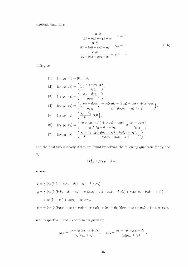
algebraic equations:
α1x
xz + b1x+ c1z + d1− x = 0,
α2y
yx+ b2y + c2x+ d2− γ2y = 0,
α3z
zy + b3z + c3y + d3− γ3z = 0.
(3.6)
This gives
(1) (x1, y1, z1) = (0, 0, 0),
(2) (x2, y2, z2) =
(0, 0,
α3 − d3γ3
b3γ3
),
(3) (x3, y3, z3) =
(0,α2 − d2γ2
b2γ2, 0
),
(4) (x4, y4, z4) =
(0,α2 − d2γ2
b2γ2,γ3(γ2(c3d2 − b2d3)− α2c3) + α3b2γ2
γ3(γ2(b2b3 − d2) + α2)
),
(5) (x5, y5, z5) =
(α1 − d1
b1, 0, 0
),
(6) (x6, y6, z6) =
(γ3(b3(α1 − d1) + c1d3)− α3c1
γ3(b1b3 − d3) + α3, 0,
α3 − d3γ3
b3γ3
),
(7) (x7, y7, z7) =
(α1 − d1
b1,γ2(c2(d1 − α1)− b1d2) + α2b1
γ2(α1 + b1b2 − d1), 0
),
and the final two x steady states are found by solving the following quadratic for x8 and
x9:
ζx28,9 + ρx8,9 + φ = 0,
where
ζ = γ2(γ3(b1b3 + c2c3 − d3) + α3 − b1c2γ2),
ρ = γ2(γ3(b3(b1b2 + d1 − α1) + c1(c2c3 − d3) + c3d2 − b2d3) + γ2(α1c2 − b1d2 − c2d1)
+ α3(b2 + c1) + α2b1)− α2c2γ3,
φ = γ2(γ3(b2(b3(d1 − α1)− c1d3) + c1c3d2) + (α1 − d1)(d2γ2 − α2) + α3b2c1)− α2c1c3γ3,
with respective y and z components given by
y8,9 =α2 − γ2(c2x8,9 + d2)
γ2(x8,9 + b2), z8,9 =
α3 − γ3(c3y8,9 + d3)
γ3(y8,9 + b3).
46

Now that we have explicit formulae for steady states (1)-(7) and implicit forms for the
final two steady states, we can use these to perform the stability analysis in terms of the
system parameters.
3.3 Analysis of the Delayed Repressilator with
Auto-activation Model (DRAM)
The equation for eigenvalues λ of the linearisation near a steady state (x, y, z) of system
(3.4) has the form
(α1(c1z + d1)e−λτx
(xz + b1x+ c1z + d1)2− 1− λ
)(α2(c2x+ d2)e−λτy
(yx+ b2y + c2x+ d2)2− γ2 − λ
)(α3(c3y + d3)e−λτz
(zy + b3z + c3y + d3)2− γ3 − λ
)−(
α1x(x+ c1)e−λτx
(xz + b1x+ c1z + d1)2
)(α2y(y + c2)e−λτy
(yx+ b2y + c2x+ d2)2
)(α3z(z + c3)e−λτz
(zy + b3z + c3y + d3)2
)= 0.
(3.7)
For the zero steady state (x, y, z) = (0, 0, 0), equation (3.7) simplifies to
(α1
d1e−λτx − 1− λ
)(α2
d2e−λτy − γ2 − λ
)(α3
d3e−λτz − γ3 − λ
)= 0. (3.8)
For the non-zero steady states, substitutions can be made to simplify analysis of the
characteristic equation (3.7). Using the system of equations (3.6), we have
xz + b1x+ c1z + d1 = α1,
yx+ b2y + c2x+ d2 = α2/γ2,
zy + b3z + c3y + d3 = α3/γ3,
so that the characteristic equation for non-zero steady states reads
(c1z + d1
α1e−λτx − 1− λ
)(γ2
2(c2x+ d2)
α2e−λτy − γ2 − λ
)(γ2
3(c3y + d3)
α3e−λτz − γ3 − λ
)−(x(x+ c1)
α1e−λτx
)(γ2
2 y(y + c2)
α2e−λτy
)(γ2
3 z(z + c3)
α3e−λτz
)= 0. (3.9)
47

3.3.1 Stability of Steady States with a Zero Component
First we look at the characteristic equation (3.8) for the zero steady state, (x1, y1, z1) =
(0, 0, 0). In the limit τx = τy = τz = 0, equation (3.8) reduces to
(α1
d1− 1− λ
)(α2
d2− γ2 − λ
)(α3
d3− γ3 − λ
)= 0,
which gives the following result.
Lemma 3.1. Let τx = τy = τz = 0. The steady state (x1, y1, z1) = (0, 0, 0) of system (3.4)
is stable whenever the following conditions hold:
i) α1 < d1,
ii) α2 < γ2d2,
iii) α3 < γ3d3.
We now assume that the conditions in Lemma 3.1 hold and analyse whether stability
can be lost as τx, τy, and τz increases. To investigate whether this steady state loses
stability for τx > 0, τy > 0, τz > 0 one can note that λ = 0 is not a root of the
characteristic equation (3.8). Therefore, the only way the steady state (x1, y1, z1) can lose
stability is if a pair of complex conjugate eigenvalues cross the imaginary axis. Hence,
we can look for solutions of (3.8) of the form λ = iω, with real ω > 0. We investigate
the possible choices of τx, τy and τz, starting with the limit τy = τz = 0, and τx > 0, to
see whether the steady state (x1, y1, z1) can lose stability. In the limit τy = τz = 0, and
τx > 0, equation (3.8) reduces to
(α1
d1e−λτx − 1− λ
)(α2
d2− γ2 − λ
)(α3
d3− γ3 − λ
)= 0.
Since Lemma 3.1 is satisfied the only way the steady state (x1, y1, z1) can lose stability is
if a pair of complex conjugate roots of α1d1e−λτx − 1 − λ = 0 crosses the imaginary axis.
48
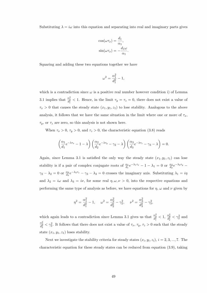
Substituting λ = iω into this equation and separating into real and imaginary parts gives
cos(ωτx) =d1
α1,
sin(ωτx) = −d1ω
α1.
Squaring and adding these two equations together we have
ω2 =α2
1
d21
− 1,
which is a contradiction since ω is a positive real number however condition i) of Lemma
3.1 implies thatα21
d21< 1. Hence, in the limit τy = τz = 0, there does not exist a value of
τx > 0 that causes the steady state (x1, y1, z1) to lose stability. Analogous to the above
analysis, it follows that we have the same situation in the limit where one or more of τx,
τy, or τz are zero, so this analysis is not shown here.
When τx > 0, τy > 0, and τz > 0, the characteristic equation (3.8) reads
(α1
d1e−λτx − 1− λ
)(α2
d2e−λτy − γ2 − λ
)(α3
d3e−λτz − γ3 − λ
)= 0.
Again, since Lemma 3.1 is satisfied the only way the steady state (x1, y1, z1) can lose
stability is if a pair of complex conjugate roots of α1d1e−λ1τx − 1 − λ1 = 0 or α2
d2e−λ2τy −
γ2 − λ2 = 0 or α3d3e−λ3τz − γ3 − λ3 = 0 crosses the imaginary axis. Substituting λ1 = iη
and λ2 = iω and λ3 = iν, for some real η, ω, ν > 0, into the respective equations and
performing the same type of analysis as before, we have equations for η, ω and ν given by
η2 =α2
1
d21
− 1, ω2 =α2
2
d22
− γ22 , ν2 =
α23
d23
− γ23 ,
which again leads to a contradiction since Lemma 3.1 gives us thatα21
d21< 1,
α22
d22< γ2
2 and
α23
d23< γ2
3 . It follows that there does not exist a value of τx, τy, τz > 0 such that the steady
state (x1, y1, z1) loses stability.
Next we investigate the stability criteria for steady states (xi, yi, zi), i = 2, 3, ..., 7. The
characteristic equation for these steady states can be reduced from equation (3.9), taking
49

Figure 3.3: Parameter regions for stable and unstable steady states of DRAM system(3.4). Each colour coded number is the indice of the corresponding steady state which isstable in that region, whilst all other steady states are unstable or infeasible. The blueregion labelled 0 is where all steady states are unstable, leading to sustained oscillations.Parameter values: τx = τy = τz = 0, α3 = 6, b1 = 4, b2 = 3, b3 = 1, c1 = 8, c2 = 10,c3 = 15, d1 = 0.5, d2 = 2, d3 = 0.2, γ2 = 0.8, γ3 = 2.
the form
(c1z + d1
α1e−λτx − 1− λ
)(γ2
2(c2x+ d2)
α2e−λτy − γ2 − λ
)(γ2
3(c3y + d3)
α3e−λτz − γ3 − λ
)= 0.
(3.10)
First we investigate (x2, y2, z2), so that equation (3.10) reduces to
(c1(α3 − γ3d3) + b3γ3d1
α1b3γ3e−λτx − 1− λ
)(γ2
2d2
α2e−λτy − γ2 − λ
)(γ2
3d3
α3e−λτz − γ3 − λ
)= 0.
In the limit τx = τy = τz = 0, the characteristic equation is given by
(c1(α3 − γ3d3) + b3γ3d1
α1b3γ3− 1− λ
)(γ2
2d2
α2− γ2 − λ
)(γ2
3d3
α3− γ3 − λ
)= 0,
Lemma 3.2. Let τx = τy = τz = 0. The steady state (x2, y2, z2) of system (3.4) is stable
whenever the following conditions hold:
i) c1(α3 − γ3d3) < b3γ3(α1 − d1),
ii) γ2d2 < α2,
iii) γ3d3 < α3.
50

0 50 100 150 200time t
0
1
2
3
(a)
x(t)y(t)z(t)
0 40 80time t
0
1
2
3
(b)
x(t)y(t)z(t)
Figure 3.4: Numerical solutions of DRAM system (3.4): (a) α1 = 13. (b) α1 = 25.Parameter values: τx = τy = τz = 0, α2 = 17, α3 = 6, b1 = 4, b2 = 3, b3 = 1, c1 = 8,c2 = 10, c3 = 15, d1 = 0.5, d2 = 2, d3 = 0.2, γ2 = 0.8, γ3 = 2.
Assuming Lemma 3.2 is satisfied, we investigate whether the steady state can lose stability
for possible choices of τx, τy, and τz. In the limit τy = τz = 0 and τx > 0, the only way
the steady state (x2, y2, z2) can lose stability is if a pair of complex conjugate eigenvalues
of c1(α3−d3γ3)+b3γ3d1α1b3γ3
e−λτx − 1−λ = 0 crosses the imaginary axis. Substituting λ = iω into
this equation and separating into real and imaginary parts we have
cos(ωτx) =α1b3γ3
c1(α3 − γ3d3) + b3γ3d1,
sin(ωτx) = − α1b3γ3ω
c1(α3 − γ3d3) + b3γ3d1.
Squaring and adding these equations together yields
ω2 =
(c1(α3 − γ3d3) + b3γ3d1
α1b3γ3
)2
− 1,
which, similarly to the steady state (x1, y1, z1), leads to a contradiction as a result of i)
and iii) in Lemma 3.2. This result shows that in the limit τy = τz = 0, there does not
exist a value of τx > 0 where the steady state (x2, y2, z2) experiences a loss of stability.
The same result arises for all other choices of τx, τy and τz, and also holds true for all
steady states (xi, yi, zi) where i = 3, 4, ..., 7. Assuming that the conditions for stability in
the limit τx = τy = τz = 0 are satisfied, each steady state remains stable for any time
delay.
Figures 3.3, 3.5, 3.6, and 3.7 represent steady state stability regions of system (3.4)
51

Figure 3.5: Parameter regions for stable and unstable steady states of DRAM system(3.4). Each colour coded number is the indice of the corresponding steady state which isstable in that region, whilst all other steady states are unstable or infeasible. The blueregion labelled 0 is where all steady states are unstable, leading to sustained oscillations.Parameter values: τx = τy = τz = 0, α1 = 4, α2 = 5, α3 = 6, b1 = 4, b2 = 3, b3 = 1,c3 = 15, d1 = 0.5, d2 = 2, d3 = 0.2, γ2 = 0.8, γ3 = 2.
Figure 3.6: Parameter regions for stable and unstable steady states of DRAM system(3.4). Each colour coded number is the indice of the corresponding steady state which isstable in that region, whilst all other steady states are unstable or infeasible. The blueregion labelled 0 is where all steady states are unstable, leading to sustained oscillations.Parameter values: τx = τy = τz = 0, α1 = 4, α2 = 5, α3 = 6, b1 = 4, b2 = 3, b3 = 1,c1 = 8, c2 = 10, c3 = 15, d3 = 0.2, γ2 = 0.8, γ3 = 2.
for the DRAM model, however the time delays have been equated to zero. These plots
therefore depict the stability regions for the ODE description of the Repressilator with
auto-activation. The numbers assigned to each colour coded region are the indices of the
respective steady state, i.e. 1 = (x1, y1, z1), 2 = (x2, y2, z2), . . . , 9 = (x9, y9, z9). The
52

parameter regions that are represented by these colours signify where the corresponding
steady state is stable. For example, if a region is colour coded with the number 2 then
this means that steady state (x2, y2, z2) is stable and all other steady states are either
unstable or biologically infeasible in this region. The dark blue coloured regions labelled
0 are areas where system parameter choices that lie here lead to instability of all steady
states, and give rise to oscillatory solutions.
In Figure 3.3, we can observe how the relationship between parameters α1 and α2 can
lead to the destabilisation of steady state (x9, y9, z9). For example if we fix α2 = 17 the
system undergoes a Hopf bifurcation as α1 is increased through α1 = 8.4. The system then
reverts back as α1 is increased beyond α1 = 18.28, to the stable steady state (x9, y9, z9). We
can also observe stability switching between many of the possible steady states throughout
the parameter space. Figure 3.4 shows two solution diagrams. The parameter scheme for
Figure 3.4(a) lies in the 0 region of Figure 3.3, and Figure 3.4(b) lies just to the right
of the 0 region. In Figure 3.4(a) we see sustained oscillations around the steady state
(x9, y9, z9), then in Figure 3.4(b) we have a solution that tends towards the stable steady
state (x9, y9, z9).
In Figure 3.5 we see a strong dependence between parameters c1 and c2 for stability
of steady states. For stability, either both parameters must be reasonably small or else if
one grows, the other must remain small. We see therefore, a large parameter region exists
where all steady states are unstable, and oscillations occur. Therefore, the model is not
robust against variations in parameters c1 and c2 with regards to steady state stability.
Figure 3.6 shows that for d2 < 5.69, the steady state (x9, y9, z9) gains stability as d1
is increased, followed by a subsequent switch of stability to (x7, y7, z7) and then a switch
to (x3, y3, z3). For 5.69 < d2 < 5.82, as d1 is increased, the steady states are unstable
followed by a gain in stability of (x9, y9, z9) for a very small parameter region before steady
state (x4, y4, z4) becomes stable and stays stable for any larger d1. For 5.82 < d2 < 6.25,
(x4, y4, z4) is stable for any choice of parameter d1, and likewise for (x2, y2, z2) when
d2 > 6.25.
In a similar fashion to Figure 3.3, Figure 3.7 shows a small pocket in the parameter
space where all steady states are unstable. This means that close to this region, if we
increase γ2, the steady state (x9, y9, z9) switches from stable to unstable and then stable
53

Figure 3.7: Parameter regions for stable and unstable steady states of DRAM system(3.4). Each colour coded number is the indice of the corresponding steady state which isstable in that region, whilst all other steady states are unstable or infeasible. The blueregion labelled 0 is where all steady states are unstable, leading to sustained oscillations.Parameter values: τx = τy = τz = 0, α1 = 4, α2 = 5, α3 = 6, b1 = 4, b2 = 3, b3 = 1,c1 = 8, c2 = 10, c3 = 15, d1 = 0.5, d2 = 2, d3 = 0.2.
again. In the rest of the parameter space we notice switches of stability between the
different steady states, so it can be inferred that the relationship between the parameters
γ2 and γ3, i.e. the degradation rates of proteins y and z, have a strong impact on the long
term behaviour of the system.
Even without time delays present it is not possible for any of the steady states
(x1, y1, z1), (x2, y2, z3), . . . , (x7, y7, z7) to undergo a Hopf bifurcation and lose stability
by varying the system parameters. The rest of this chapter investigates the stability prop-
erties of the remaining two steady states and the effect that time delays have on the long
term system behaviour.
3.3.2 Stability of Steady States with Non-zero Components
We wish to investigate stability of the steady states (x8, y8, z8) and (x9, y9, z9), which have
non zero values in all components. Here, the number of free parameters of system (3.4) is
reduced in order to simplify analysis of the DRAM model which has 3 time delays. From
here on, it is assumed that protein x is a different type to proteins y and z. Protein x is
expressed under a smaller time scale to y and z, such that the time delays associated with
protein x are negligible, relative to the delays associated with proteins y and z. Thus, we
take the limit τx = 0 and relabel τy = τ1 and τz = τ2. The system of equations for this
54

model is then given by
dx
dt=
α1x
xz + b1 + c1 + d1− x,
dy
dt=
α2y(t− τ1)
y(t− τ1)x(t− τ1) + b2y(t− τ1) + c2x(t− τ1) + d2− γ2y,
dz
dt=
α3z(t− τ2)
z(t− τ2)y(t− τ2) + b3z(t− τ2) + c3y(t− τ2) + d3− γ3z.
(3.11)
This model will be referred to as the simplified delayed repressilator with auto-activation
model (SDRAM). The initial conditions for model SDRAM are
x(s) = φ1(s), s ∈ [−τmax, 0],
y(s) = φ2(s), s ∈ [−τmax, 0],
z(s) = φ3(s), s ∈ [−τmax, 0],
where τmax = max(τ1, τ2) and φi(s) ∈ C([−τmax, 0],R) with φi(s) ≥ 0 (−τmax ≤ s ≤ 0,
i = 1, 2, 3). C([−τmax, 0],R) is the Banach space of continuous mappings of interval
[−τmax, 0] into R. It is also assumed that x(0) > 0, y(0) > 0, and z(0) > 0. The proof
for the positivity of solutions follows the same methodology to that of system (3.4). Since
time delays have no affect on the calculation of steady states, the equilibria of system
(3.11) are the same as for system (3.4). Therefore, to investigate the stability properties
of (x8, y8, z8) and (x9, y9, z9) with respect to the new reduced system, the characteristic
equation of system (3.11) for non-zero steady states reads
(c1z + d1
α1− 1− λ
)(γ2
2(c2x+ d2)
α2e−λτ1 − γ2 − λ
)(γ2
3(c3y + d3)
α3e−λτ2 − γ3 − λ
)−(x(x+ c1)
α1
)(γ2
2 y(y + c2)
α2e−λτ1
)(γ2
3 z(z + c3)
α3e−λτ2
)= 0
⇔ λ3 + λ2(1 + γ2 + γ3 − κ1 − κ2e−λτ1 − κ3e
−λτ2) + λ((κ1 − γ3 − 1)κ2e−λτ1
+ (κ1 − γ2 − 1)κ3e−λτ2 + κ2κ3e
−λ(τ1+τ2) + γ2 + γ3 + γ2γ3 − κ1(γ2 + γ3))
+ (κ1 − 1)(γ3κ2e−λτ1 + γ2κ3e
−λτ2 − κ2κ3e−λ(τ1+τ2) − γ2γ3) + ξ1ξ2ξ3e
−λ(τ1+τ2) = 0,
(3.12)
55
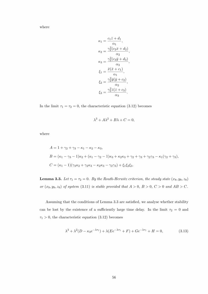
where
κ1 =c1z + d1
α1,
κ2 =γ2
2(c2x+ d2)
α2,
κ3 =γ2
3(c3y + d3)
α3,
ξ1 =x(x+ c1)
α1,
ξ2 =γ2
2 y(y + c2)
α2,
ξ3 =γ2
3 z(z + c3)
α3.
In the limit τ1 = τ2 = 0, the characteristic equation (3.12) becomes
λ3 +Aλ2 +Bλ+ C = 0,
where
A = 1 + γ2 + γ3 − κ1 − κ2 − κ3,
B = (κ1 − γ3 − 1)κ2 + (κ1 − γ2 − 1)κ3 + κ2κ3 + γ2 + γ3 + γ2γ3 − κ1(γ2 + γ3),
C = (κ1 − 1)(γ3κ2 + γ2κ3 − κ2κ3 − γ2γ3) + ξ1ξ2ξ3.
Lemma 3.3. Let τ1 = τ2 = 0. By the Routh-Herwitz criterion, the steady state (x8, y8, z8)
or (x9, y9, z9) of system (3.11) is stable provided that A > 0, B > 0, C > 0 and AB > C.
Assuming that the conditions of Lemma 3.3 are satisfied, we analyse whether stability
can be lost by the existence of a sufficiently large time delay. In the limit τ2 = 0 and
τ1 > 0, the characteristic equation (3.12) becomes
λ3 + λ2(D − κ3e−λτ1) + λ(Ee−λτ1 + F ) +Ge−λτ1 +H = 0, (3.13)
56

where
D = 1 + γ2 + γ3 − κ1 − κ3,
E = κ2(κ1 + κ3 − γ3 − 1),
F = κ3(κ1 − γ2 − 1) + γ2 + γ3 + γ2γ3 − κ1(γ2 + γ3),
G = κ2(κ1 − 1)(γ3 − κ3) + ξ1ξ2ξ3,
H = γ2(κ1 − 1)(κ3 − γ3).
We look for solutions of (3.13) of the form λ = iω for some real ω > 0. Substituting this
into (3.13) and separating into real and imaginary parts we have
Dω2 −H = (κ3ω2 +G) cos(ωτ1) + Eω sin(ωτ1),
ω(F − ω2) = (κ3ω2 +G) sin(ωτ1)− Eω cos(ωτ1).
(3.14)
Squaring and adding together gives a cubic equation of the form:
g(z) = z3 + pz2 + qz + r = 0, (3.15)
where z = ω2 and
p = D2 − 2F − κ23,
q = F 2 − 2DH − 2Gκ3 − E2,
r = H2 −G2.
Without loss of generality, suppose that (3.15) has 3 positive real roots, denoted by z1, z2,
z3, respectively, which would give 3 possible values of ω: ω1 =√z1, ω2 =
√z2, ω3 =
√z3.
Some algebraic manipulation of (3.14) gives
cos(ωkτ1,k) =(E + κ3)ω4
k + (DG− EF −Hκ3)ω2k −GH
κ23ω
4k + (E2 + 2Gκ3)ω2
k +G2
⇒ τ1,k,j =1
ωk
[arccos
((E + κ3)ω4
k + (DG− EF −Hκ3)ω2k −GH
κ23ω
4k + (E2 + 2Gκ3)ω2
k +G2
)+ 2jπ
],
k = 1, ..., 3, j = 0, 1, 2, ....
57

Define,
τ1,0 = min1≤k≤3
{τ1,k,0}, ω0 = ωk0 , k0 ∈ {1, 2, 3},
then τ1,0 is the first value of τ1 > 0 whereby the characteristic equation (3.13) has a pair
of purely imaginary roots. We have the following result.
Theorem 3.1 Suppose the conditions of Lemma 3.3 hold and that g′(ω2) > 0, where g(z)
is defined in (3.15). In the limit τ2 = 0, the steady state (x8, y8, z8) or (x9, y9, z9) of
system (3.11) is stable for 0 ≤ τ1 ≤ τ1,0 and unstable for τ1 > τ1,0 and undergoes a Hopf
bifurcation at τ1 = τ1,0.
Proof. The conclusion of Lemma 3.3 ensures that the steady state (x8, y8, z8) or (x9, y9, z9)
of system (3.11) is stable at τ1 = 0, and the fact that the roots of the characteristic
equation (3.13) depend continuously on τ1 implies that either steady state is also stable
for sufficiently small positive values of τ1. Since τ1,0 is the first positive τ1, for which the
eigenvalues lie on the imaginary axis, in order to verify whether or not the steady state
actually loses stability at τ1 = τ1,0, one has to compute the sign of dRe(λ)/dτ1|τ1=τ1,0 .
Let λ(τ1) = µ(τ1) + iω(τ1) be the root of the characteristic equation (3.13) near τ1 =
τ1,0, satisfying µ(τ1,0) = 0 and ω(τ1,0) = ω0. Substituting λ = λ(τ1) into (3.13) and
differentiating both sides with respect to τ1 yields
(dλ
dτ1
)−1
=(3λ2 + 2Dλ+ F )eλτ1
λ(−κ3λ2 + Eλ+G)+
E − 2κ3λ
λ(−κ3λ2 + Eλ+G)− τ1
λ.
From this equation, one can find
sgn
{[d(Reλ)
dτ1
]τ1=τ1,0
}= sgn
Re
[(dλ
dτ1
)−1]τ1=τ1,0
58
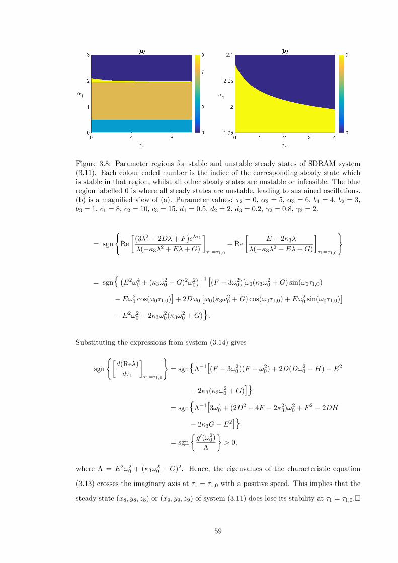
Figure 3.8: Parameter regions for stable and unstable steady states of SDRAM system(3.11). Each colour coded number is the indice of the corresponding steady state whichis stable in that region, whilst all other steady states are unstable or infeasible. The blueregion labelled 0 is where all steady states are unstable, leading to sustained oscillations.(b) is a magnified view of (a). Parameter values: τ2 = 0, α2 = 5, α3 = 6, b1 = 4, b2 = 3,b3 = 1, c1 = 8, c2 = 10, c3 = 15, d1 = 0.5, d2 = 2, d3 = 0.2, γ2 = 0.8, γ3 = 2.
= sgn
{Re
[(3λ2 + 2Dλ+ F )eλτ1
λ(−κ3λ2 + Eλ+G)
]τ1=τ1,0
+ Re
[E − 2κ3λ
λ(−κ3λ2 + Eλ+G)
]τ1=τ1,0
}
= sgn{ (E2ω40 + (κ3ω
20 +G)2ω2
0
)−1 [(F − 3ω20)[ω0(κ3ω
20 +G) sin(ω0τ1,0)
− Eω20 cos(ω0τ1,0)] + 2Dω0
[ω0(κ3ω
20 +G) cos(ω0τ1,0) + Eω2
0 sin(ω0τ1,0)]
− E2ω20 − 2κ3ω
20(κ3ω
20 +G)}.
Substituting the expressions from system (3.14) gives
sgn
{[d(Reλ)
dτ1
]τ1=τ1,0
}= sgn{Λ−1[(F − 3ω2
0)(F − ω20) + 2D(Dω2
0 −H)− E2
− 2κ3(κ3ω20 +G)]}
= sgn{Λ−1[3ω40 + (2D2 − 4F − 2κ2
3)ω20 + F 2 − 2DH
− 2κ3G− E2]}= sgn
{g′(ω2
0)
Λ
}> 0,
where Λ = E2ω20 + (κ3ω
20 + G)2. Hence, the eigenvalues of the characteristic equation
(3.13) crosses the imaginary axis at τ1 = τ1,0 with a positive speed. This implies that the
steady state (x8, y8, z8) or (x9, y9, z9) of system (3.11) does lose its stability at τ1 = τ1,0.�
59

Figure 3.8 demonstrates how increasing the time delay τ1 results in a Hopf bifurcation
of the steady state (x9, y9, z9) and the emergence of a stable periodic orbit. For 0 < α1 <
0.5058 and 0.5058 < α1 < 1.963, steady state (x3, y3, z3) and (x7, y7, z7), respectively,
are stable for any time delay. However for 1.963 < α1 < 2.083, there exists a critical
time delay which leads to sustained oscillations when τ1 passes this value. In accordance
with Theorem 3.1, once the stability of the steady state (x9, y9, z9) is lost, it can never
be regained for higher values of τ , so the system will be exhibiting oscillatory behaviour.
Beyond α1 = 2.083 the steady states are unstable for all τ1.
In the limit τ1 = 0 with τ2 > 0, the story is identical to the limit τ2 = 0 with τ1 > 0, so
this analysis has not been included here. Next we look at the case where τ1 = τ2 = τ > 0.
The characteristic equation is given by
λ3 + λ2(I − Je−λτ ) + λ(Ke−λτ + Le−2λτ +M) +Ne−λτ + Pe−2λτ +Q = 0, (3.16)
where
I = 1 + γ2 + γ3 − κ1,
J = κ2 + κ3,
K = κ2(κ1 − γ3 − 1) + κ3(κ1 − γ2 − 1),
L = κ2κ3,
M = γ2 + γ3 + γ2γ3 − κ1(γ2 + γ3),
N = (κ1 − 1)(γ3κ2 + γ2κ3),
P = κ2κ3(1− κ1) + ξ1ξ2ξ3,
Q = γ2γ3(1− κ1).
Here we use an iterative procedure adopted from B. Rahman et al. [130] to find a new
function F (ω), the roots of which give the Hopf frequency associated with the purely
imaginary roots of the characteristic equation (3.16). The procedure we employ for find-
ing the function F (ω) works as follows. Consider a general transcendental characteristic
60

equation [131–133],
∆(τ, λ) =
n∑k=0
pk(λ)e−kλτ , (3.17)
where τ ≥ 0; pk(λ), k = 0, 1, 2, ..., are polynomials in λ; and |pk(λ)/p0(λ)| < 1, k =
1, 2, ..., n, for |λ| → ∞ and Re(λ) ≥ 0. Substituting λ = iω into (3.17) and conjugating
∆(τ, iω) gives
∆(τ, iω) =
n∑k=0
pk(iω)e−kiωτ , ∆(τ, iω) =
n∑k=0
pk(iω)ekiωτ .
Clearly, ∆(τ, iω) = 0 if and only if ∆(τ, iω) = 0. Define ∆(j)(τ, iω) recursively as
∆(1)(τ, iω) = p0(iω)∆(τ, iω)− pn(iω)e−niωτ∆(τ, iω) =n−1∑k=0
p(1)k (iω)e−kiωτ ,
...
∆(j)(τ, iω) = p(j−1)0 (iω)∆(j−1)(τ, iω)− p(j−1)
n−j+1(iω)e−(n−j+1)iωτ∆(j−1)(τ, iω)
=
n−j∑k=0
p(j)k (iω)e−kiωτ ,
...
∆(n−1)(τ, iω) = p(n−1)0 (iω) + p
(n−1)1 (iω)e−iωτ .
From p(j+1)0 (iω) we obtain
p(j+1)0 (iω) = |p(j)
0 (iω)|2 − |p(j)n−j(iω)|2, j = 0, 1, 2, ..., n− 2.
Moreover, from ∆(n−1)(τ, iω), let
F (ω) = |p(n−1)0 (iω)|2 − |p(n−1)
1 (iω)|2.
If ∆(τ, iω) = 0, then ω is a root of F (ω) = 0.
Now returning to (3.16) one can use the same argument as above with n = 2 to find
the function F (ω):
F (ω) = |p10(iω)|2 − |p1
1(iω)|2,
61

where
p10(iω) = ω6 + (I2 − 2M)ω4 + (M2 − L2 − 2IQ)ω2 +Q2 − P 2, (3.18)
p11(iω) =− (IJ +K)ω4 + (J(Q− P ) +K(M − L)− IN)ω2 +N(Q− P )
+ i[Jω5 + (N − J(L+M)− IK)ω3 + (K(P +Q)−N(L+M))ω].
The function F (ω) is then calculated to give
F (ω) = ω12 +A1ω10 +A2ω
8 +A3ω6 +A4ω
4 +A5ω2 +A6, (3.19)
where,
A1 = 2I2 − J2 − 4M,
A2 = I4 − (J2 + 4M)I2 + 2[J(J(L+M)−N) + 3M2 − 2IQ− L2]−K2,
A3 =− 4I3Q+ [2(M2 − JN − L2)−K2]I2 + 2[J(J(Q− P )− 2KL) + 4MQ]I
− 4M3 − J2M2 + 2[J(2N − JL) +K2 + 2L2]M + J [4(LN −KP )− JL2]
− 2(K2L+ P 2)−N2 + 2Q2,
A4 = M4 − [2(2IQ+ JN + L2) +K2]M2 + 2[K2L+N2 − 2Q2 + 2(J(KP − LN)
+ P 2)]M + (6Q2 −N2 − 2P 2)I2 + 2[K2(P +Q) + 2L2Q+ 2N(J(Q− P )−KL)]I
+ L4 − (2JN +K2)L2 + 2(2JKQ+N2)L+ J2[P (2Q− P )−Q2]− 4KNP,
A5 = [2(I(Q− P )− LM)− L2 −M2]N2 + 2[2(Q(JP +KL) +KMP )− J(P 2 +Q2)]N
+ 2P 2(2IQ+ L2 −M2)−K2(P +Q)2 + 2Q2(M2 − L2 − 2IQ),
A6 = (P 2 −Q2)2 −N2(P −Q)2.
If A6 < 0 in (3.19), then the function F (ω) has at least one positive root, ω, satisfying
F (ω) = 0. We can prove this as follows. Assuming A6 < 0 implies that F (0) = A6 < 0.
Since F (ω) is a continuous function of ω, and also limω→∞ F (ω) = ∞, this means there
exists a positive root ω > 0 such that F (ω) = 0.
We now consider the case where A6 ≥ 0. Let z = ω2, then the equation F (ω) = 0 can
62

be written as
h(z) = z6 +A1z5 +A2z
4 +A3z3 +A4z
2 +A5z +A6 = 0. (3.20)
Without loss of generality, suppose that (3.20) has six positive real roots denoted by z1,
z2, z3, z4, z5, z6, respectively, which would give six possible values of ω:
ω1 =√z1, ω2 =
√z2, ω3 =
√z3, ω4 =
√z4, ω5 =
√z5, ω6 =
√z6.
Now looking for solutions of (3.16) of the form λ = iω for some real ω > 0, and separating
into real and imaginary parts we have
(Jω2 +N) cos(ωτ) +Kω sin(ωτ) = Iω2 −Q− [P cos(2ωτ) + Lω sin(2ωτ)],
−(Jω2 +N) sin(ωτ) +Kω cos(ωτ) = ω(ω2 −M) + P sin(2ωτ)− Lω cos(2ωτ).
Squaring and adding together gives
β cos(u) + δ sin(u) = ε,
where
u = 2ωτ,
β = 2[P (Iω2 −Q) + Lω2(ω2 −M)],
δ = 2ω[P (M − ω2) + L(Iω2 −Q)],
ε = (Iω2 −Q)2 + ω2(ω2 −M)2 + ω2(L2 −K2) + P 2 − (Jω2 +N)2.
Dividing by√β2 + δ2 we obtain
β cos(u)√β2 + δ2
+δ sin(u)√β2 + δ2
=ε√
β2 + δ2. (3.21)
Note that, (β√
β2 + δ2
)2
+
(δ√
β2 + δ2
)2
= 1.
63

Hence, there must exist a value θ such that
cos(θ) =β√
β2 + δ2, sin(θ) =
δ√β2 + δ2
, and θ = arctan
(δ
β
).
Thus we can rewrite (3.21) as follows:
cos(u) cos(θ) + sin(u) sin(θ) =ε√
β2 + δ2
⇔ cos(u− θ) =ε√
β2 + δ2.
Through some algebraic manipulation we are able to find the critical time delays given by
τk,j =1
2ωk
arctan
(δkβk
)+ arccos
εk√β2k + δ2
k
+ jπ
,k = 1, 2, . . . , 6, j = 0, 1, 2, . . . .
Define,
τ0 = min1≤k≤6
τk,0, ω0 = ωk0 , k0 ∈ {1, 2, 3, 4, 5, 6},
then τ0 is the first value of τ > 0 such that the characteristic equation (3.16) has a
pair of purely imaginary roots. We can state some implicit conditions on whether a Hopf
bifurcation arises at the critical time delay by looking to prove the transversality condition.
Let λ(τ) = µ(τ) + iω(τ) be the root of the characteristic equation (3.16) near τ = τ0,
satisfying µ(τ0) = 0 and ω(τ0). Substituting λ = λ(τ) into (3.16) and differentiating both
sides with respect to τ yields
(dλ
dτ
)−1
=3λ2 + 2Iλ+M + (K − 2Jλ)e−λτ + Le−2λτ
λ[(−Jλ2 +Kλ+N)e−λτ + (2Lλ+ 2P )e−2λτ ]− τ
λ.
64
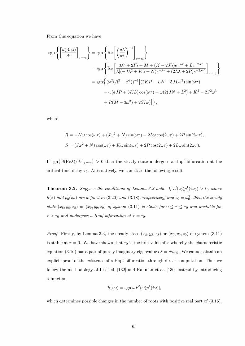
From this equation we have
sgn
{[d(Reλ)
dτ
]τ=τ0
}= sgn
{Re
[(dλ
dτ
)−1]τ=τ0
}
= sgn
{Re
[3λ2 + 2Iλ+M + (K − 2Jλ)e−λτ + Le−2λτ
λ[(−Jλ2 +Kλ+N)e−λτ + (2Lλ+ 2P )e−2λτ ]
]τ=τ0
}
= sgn{(ω2(R2 + S2))−1[(2KP − LN − 5JLω2) sin(ωτ)
− ω(4JP + 3KL) cos(ωτ) + ω(2(JN + L2) +K2 − 2J2ω3
+R(M − 3ω2) + 2SIω)]},
where
R = −Kω cos(ωτ) + (Jω2 +N) sin(ωτ)− 2Lω cos(2ωτ) + 2P sin(2ωτ),
S = (Jω2 +N) cos(ωτ) +Kω sin(ωτ) + 2P cos(2ωτ) + 2Lω sin(2ωτ).
If sgn{[d(Reλ)/dτ ]τ=τ0} > 0 then the steady state undergoes a Hopf bifurcation at the
critical time delay τ0. Alternatively, we can state the following result.
Theorem 3.2. Suppose the conditions of Lemma 3.3 hold. If h′(z0)p10(iω0) > 0, where
h(z) and p10(iω) are defined in (3.20) and (3.18), respectively, and z0 = ω2
0, then the steady
state (x8, y8, z8) or (x9, y9, z9) of system (3.11) is stable for 0 ≤ τ ≤ τ0 and unstable for
τ > τ0 and undergoes a Hopf bifurcation at τ = τ0.
Proof. Firstly, by Lemma 3.3, the steady state (x8, y8, z8) or (x9, y9, z9) of system (3.11)
is stable at τ = 0. We have shown that τ0 is the first value of τ whereby the characteristic
equation (3.16) has a pair of purely imaginary eigenvalues λ = ±iω0. We cannot obtain an
explicit proof of the existence of a Hopf bifurcation through direct computation. Thus we
follow the methodology of Li et al. [132] and Rahman et al. [130] instead by introducing
a function
S1(ω) = sgn[ωF ′(ω)p10(iω)],
which determines possible changes in the number of roots with positive real part of (3.16).
65

Figure 3.9: Parameter regions for stable and unstable steady states of SDRAM system(3.11). Each colour coded number is the indice of the corresponding steady state whichis stable in that region, whilst all other steady states are unstable or infeasible. The blueregion labelled 0 is where all steady states are unstable, leading to sustained oscillations.Parameter values: τ2 = 15, α2 = 5, α3 = 6, b1 = 4, b2 = 3, b3 = 1, c1 = 8, c2 = 10,c3 = 15, d1 = 0.5, d2 = 2, d3 = 0.2, γ2 = 0.8, γ3 = 2.
From the definition of the function h(z), we have
F (ω) = h(ω2) ⇒ F ′(ω) = 2ωh′(ω2) = 2ωh′(z),
which, under the assumption that h′(z0)p10(iω0) > 0, implies
S1(ω0) = sgn[ω0F′(ω0)p1
0(iω0)] = sgn[2ω20h′(z0)p1
0(iω0)] = sgn[h′(z0)p10(iω0)] > 0.
From Theorem 2 in [132] we have
sgn
{[dRe[λ(τ)]
dτ
]τ=τ0
}> 0,
hence the steady state (x8, y8, z8) or (x9, y9, z9) undergoes a Hopf bifurcation at τ = τ0.�
Finally we would like to investigate, analytically, the case where τ1 6= τ2. The corre-
sponding characteristic equation is given by
λ3 + λ2(U − κ2e−λτ1 − κ3e
−λτ2) + λ(V e−λτ1 +We−λτ2 + Le−λ(τ1+τ2) +M) +Xe−λτ1
+ Y e−λτ2 + Pe−λ(τ1+τ2) +Q = 0, (3.22)
66

Figure 3.10: Parameter regions for stable and unstable steady states of SDRAM system(3.11). Each colour coded number is the indice of the corresponding steady state whichis stable in that region, whilst all other steady states are unstable or infeasible. The blueregion labelled 0 is where all steady states are unstable, leading to sustained oscillations.Parameter values: τ2 = 15, α1 = 4, α2 = 5, α3 = 6, b1 = 4, b2 = 3, b3 = 1, c2 = 10,c3 = 15, d1 = 0.5, d2 = 2, d3 = 0.2, γ2 = 0.8, γ3 = 2.
where
U = 1 + γ2 + γ3 − κ1,
V = (κ1 − γ3 − 1)κ2,
W = (κ1 − γ2 − 1)κ3,
X = (κ1 − 1)γ3κ2,
Y = (κ1 − 1)γ2κ3,
and L, M , P , Q are the same as defined for (3.16). However the number of free parame-
ters, time delays and exponential terms in the coefficients of the characteristic polynomial
on the left hand side of (3.22) makes it infeasible to perform any meaningful mathemat-
ical analysis on the characteristic equation (3.22). We leave this case to be analysed
numerically.
In Figure 3.9 the parameters are the same as in Figure 3.8, however, now τ2 is not
chosen in the limit τ2 = 0 but instead, τ2 = 15. In this scenario, notice how in the param-
eter region 1.963 < α1 < 2.309, for small τ1 all steady states are unstable but then as τ1
is increased, steady state (x9, y9, z9) experiences a diminishing switch-like behaviour be-
tween stable and unstable. Unlike Figure 3.8, when stability is lost at a critical time delay,
67

Figure 3.11: Parameter regions for stable and unstable steady states of SDRAM system(3.11). Each colour coded number is the indice of the corresponding steady state whichis stable in that region, whilst all other steady states are unstable or infeasible. The blueregion labelled 0 is where all steady states are unstable, leading to sustained oscillations.Parameter values: τ2 = 15, α1 = 4, α2 = 5, α3 = 6, b1 = 4, b2 = 3, b3 = 1, c1 = 8, c2 = 10,c3 = 15, d2 = 2, d3 = 0.2, γ2 = 0.8, γ3 = 2.
the steady state (x9, y9, z9) does not remain unstable for larger values of τ1. This result
highlights the importance of correct mathematical representation of the transcription and
translation processes, since inclusion of multiple transcriptional and translational delays
can lead to regions in the parameter space where, depending on the careful choice of time
delay values, either sustained periodic oscillations occur or the solution tends towards a
stable steady state.
Figure 3.10 looks at the stability relationship between c1 and τ1. We see that there are
only two attainable stable steady states through varying the parameter c1. In the region
of parameter space where (x6, y6, z6) is stable, it remains so for any time delay. There is
again a region in the parameter space where switching occurs between stable and unstable
steady state (x9, y9, z9) as τ1 is increased. Notice the spiking behaviour of the unstable
region for 1.195 < c1 < 1.348.
We see that Figure 3.11 appears almost as a flipped image of Figure 3.9. In the regions
of the parameter space where steady state (x3, y3, z3) or (x7, y7, z7) are stable, they remain
so for any time delay τ1. Similar to parameter α1, there exists a region 2.215 < d1 < 2.563
where if the steady state (x9, y9, z9) loses stability due to an increase in τ1, it experiences
switching behaviour between stable and unstable for larger τ1.
68

(a)
τ2
Re
Λm
ax
0 20 40τ1
0
20
40
0
0.05
0.1
0.15
(b)
τ2
Re
Λm
ax
0 40 80τ1
0
20
40
-0.03
-0.015
0
0.015
(c)
τ2R
e Λ
max
0 20 40τ1
0
20
40
-0.1
-0.05
0
(d)
τ2
Re
Λm
ax
0 20 40τ1
0
20
40
-0.01
0
0.01
0.02
Figure 3.12: The values of Max(Re(λ)) in the (τ1, τ2) parameter space for steady state(x9, y9, z9) of SDRAM system. All other steady states are either unstable or infeasible forthese parameter schemes. (a) Parameter values: α1 = 4, α2 = 5, α3 = 6, b1 = 4, b2 = 3,b3 = 1, c1 = 8, c2 = 10, c3 = 15, d1 = 0.5, d2 = 2, d3 = 0.2, γ2 = 0.8, γ3 = 2. (b) α1 = 2.(c) c1 = 1. (d) d1 = 2.4. All other parameters remain the same as (a) in (b)-(d).
Figure 3.12 shows stability regions in the (τ1, τ2) parameter space. The parameters
fixed in Figure 3.12(a) are the same as those used throughout Figures 3.8-3.11. However,
notice how the value of α1 = 4 places the parameter choice beyond the range of the y
axis in Figure 3.9, and thus it sits in the region where all steady states are unstable for
any τ1. This is also illustrated in Figure 3.12(a), the steady states are unstable for any
choices of either time delay. In Figure 3.12(b), the parameter α1 = 2 is fixed. Notice
that this parameter choice lies in the region of Figure 3.8 where steady state (x9, y9, z9)
is stable and subsequently loses stability as τ1 is increased. We see that Figure 3.12(b)
produces rich dynamics of switching between regions where steady state (x9, y9, z9) is stable
(Max(Re(λ)) < 0) and regions where all steady states are unstable (Max(Re(λ)) > 0). In
Figures 3.12(c) and 3.12(d) parameters c1 and d1 are fixed so that they lie in the regions
of Figures 3.10 and 3.11, respectively, where steady state (x9, y9, z9) is stable. All other
69

parameters remain the same. Again we see spiking regions that spread across the entire
parameter space.
In all Figures it can be seen that the losses and gains in stability all occur around
(x9, y9, z9), showing that the stability of this steady state is not robust against parameter
variations. This result is highlighted further by Figure 3.12 as it shows the sensitivity
of steady state (x9, y9, z9) to losing stability through changes in the transcriptional and
translational time delays.
3.4 Discussion
In this chapter we have discussed a mathematical model for the analysis of a GRN and
focussed on the role played by the transcriptional and translational time delays in the
dynamics of a three-gene Repressilator model with auto-activation. We have established
conditions for stability of seven equilibria and found that none of these can undergo a
switch in stability due to the existence of time delays. By reducing the model to the one
with two time delays, we could investigate the last two steady states by considering a
scenario where protein x is expressed under a smaller time scale to y and z, such that the
time delays associated with protein x are negligible. We found, analytically, the boundary
of the Hopf bifurcation depending on the two time delays and other system parameters,
and illustrated different types of behaviour by direct simulation. Mathematical analysis
has shown that only the steady states with non-zero x, y, and z components (labelled
(x8, y8, z8) and (x9, y9, z9)) have the potential to undergo a Hopf bifurcation depending
on the time delays. However numerical simulations show us that it is in fact only steady
state (x9, y9, z9) that can undergo a Hopf bifurcation as a result of increasing time delays.
Our results also suggest that under certain parameter choices, steady state (x9, y9, z9)
can alternate between stable and unstable as a time delay is increased. The numerical
simulations reveal switching between different stable steady states through variations in
the system parameters. This is in agreement with the biology, as the changes in stable
steady states can account for different cell fates of GRNs in the immune system.
70
Chapter 4
Time-Delayed Model of a Genetic
Network with Switches and
Oscillations
The two types of systems that are of particular interest in this chapter are the Repressilator
[74] and the Toggle switch [80]. As mentioned in the previous chapter, the Repressilator
is a model comprised of three genes which are connected in such a way that the protein
coded by each gene inhibits the expression of the next gene in the cycle, thus acting as a
repressor. The Toggle switch is made up of two genes with mutually repressing proteins,
which leads to bistability. Bistability is a type of switch which permits the coexistence of
two stable steady states, and is known to be a key component in biological systems such
as cell fates of GRNs during the immune response to an antigen.
The Repressilator and Toggle switch have been studied in a variety of ways [134–138],
however all of these models looked at the two systems independently of each other. A paper
by Gonze [139] looked to combine the two and unravel the compositional rules that govern
its dynamics. This type of model was warranted since biological systems are composed
of interconnected positive and negative circuits [140]. They investigated the dynamical
properties that arise through the coupling of the Repressilator and Toggle switch. Two
forms of coupling were investigated. In the first case, one protein of the Repressilator
activates the expression of one gene in the Toggle switch. In the second case, a protein
in the Toggle switch activates the expression of one gene in the Repressilator. Both types
71
are what’s known as master/slave systems, since one subsystem is under the control of
the other through unidirectional coupling. In the study, Gonze accounted for the coupling
through a linear function and it was addressed that using a more elaborate coupling
term leads to qualitatively similar results. Gonze first investigated the system where a
protein in the Repressilator activates the Toggle switch. It was shown through numerical
simulation, and using the coupling term as a bifurcation parameter, that the amplitude of
the oscillatory coupling may lead to four different dynamical behaviour scenarios. When
the amplitude of the coupling is sufficiently large, oscillations of the Repressilator are
able to induce a periodic switch in the Toggle switch. However, when the amplitude of
coupling is insufficient, a periodic switch cannot be induced. Instead, the trajectory of
the coupled protein, X, in the Toggle switch oscillates with low-amplitude around the
lower steady state. When the amplitude of coupling is very low there are two possible
scenarios. Under certain conditions it is possible for X to oscillate with low-amplitude
around the upper steady state, or a phenomenon of birythmicity occurs. Birythmicity
is where, under particular initial conditions, low-amplitude oscillations around the upper
steady state are induced, whilst under a different set of initial conditions there are low-
amplitude oscillations around the lower steady state. Gonze also investigated the effect of
the period of oscillations on the dynamical behaviour of the Toggle switch. No periodic
switch is observed given a sufficiently small period.
Investigating the second type of coupling, where the Toggle switch activates the Re-
pressilator, a transient perturbation was also considered. It was shown that an external
signal acting on the Toggle switch has the potential to induce oscillations in the Repres-
silator or in fact stop any existing oscillations. This paper by Gonze highlights how one
can obtain control, through parameter tuning and network structure, over the dynamical
behaviour of an oscillatory system coupled with a bistable switch. This is important as
unidirectional coupling is likely to be present at multiple stages of gene regulatory net-
works which were shown to be hierarchical [139]. It should be noted that bidirectional
(mutual) coupling between biological switches and oscillators also exist in many biologi-
cal networks, such as bidirectional coupling between the ATM switch and the p53-Mdm2
oscillator in the p53 signaling network [141], and this form of coupling between the Toggle
switch and Repressilator has also been studied [142].
This chapter explores the impact of transcriptional and translational delays on a five-
72
gene system with unidirectional coupling, where the expression of a gene in the Toggle
switch is under the control of a protein in the Repressilator. Although the literature
studied the effects of coupling amplitude on the oscillatory dynamics of the system, in
this chapter stability analysis is also performed to establish the conditions for a Hopf
bifurcation where solutions exhibit such oscillations. We then make a comparative analysis
between the delayed model, described using delay differential equations, and the existing
ODE model in the literature. This is done by studying the dynamical behaviours observed
in numerical simulations of the DDE system, and comparing the results to those found by
Gonze. The existence of new dynamical behaviours are shown which were impossible in
the model system without the time delays.
4.1 The Delayed Model
The Repressilator is a model composed of three genes which are cyclically connected in
such a way that the protein coded by each gene in the system acts as a repressor for
the transcription of the next gene in the cycle [139]. The dynamics of this model can be
described by the following set of ordinary differential equations:
dMi
dt= T
(−Mi +
αi1 + Pmmod(i+1,3)
), with i = 1, 2, 3,
dPidt
= T (βiMi − γiPi), with i = 1, 2, 3.
Here, Mi and Pi represent the concentrations of mRNA and protein, respectively, of the
corresponding ith gene in the system. The Hill function αi/(1 + Pmmod(i+1,3)) accounts
for the inhibition where “mod” is the modulo function. The parameter αi represents the
maximum rate of mRNA synthesis of gene i. Parameter T has been introduced to allow
us to easily control time scale of the dynamics. Variables and time have been rescaled and
adimensionalised.
The dynamics of the Toggle switch system, which consists of two genes that mutually
inhibit each other, are described by the following ODEs:
dX
dt=
a1
1 + Y n− d1X + b1,
dY
dt=
a2
1 +Xn− d2Y + b2.
73

G3
G2G1
X Y
Figure 4.1: Network motif of the Repressilator coupled with a Toggle switch. The nodesare genes G1, G2, and G3 of the Repressilator, which are connected by edges, in red,representing regulation of each gene by inhibition from the preceding gene in the cycle.The genes X and Y of the Toggle switch are connected by edges, in red, representingregulation of each gene by mutual repression. The Repressilator and Toggle switch arecoupled through an edge, in blue, connecting gene G1 with X which represents regulationof gene X by activation from G1.
There is no distinction made between the gene and the protein, unlike in the Repressilator
model. Qualitatively, the results will be the same if we were to include equations which
account for the evolution of mRNAs for X and Y . In this model, the inhibition is described
by the Hill functions a1/(1 + Y n) and a2/(1 +Xn) where a1 and a2 denote the maximum
rate of X and Y mRNA synthesis, respectively, and n is the cooperativity. Parameters
b1 and b2 describe an independent synthesis source of X and Y , resulting from another
promoter perhaps, which is unaffected by the inhibition of X and Y , but can be controlled
by external factors. Again, variables and time have been rescaled and adimensionalised.
We are interested in the type of coupling where the Repressilator is in control of the
Toggle switch, see Figure 4.1. This model, studied by Gonze [139], is given by the following
ODEs:
dMi
dt= T
(−Mi +
αi1 + Pmmod(i+1,3)
), with i = 1, 2, 3,
dPidt
= T (βiMi − γiPi), with i = 1, 2, 3,
dX
dt=
a1
1 + Y n− d1X + b1,
dY
dt=
a2
1 +Xn− d2Y + b2,
(4.1)
74

where a1 = AP1 + B is the linear coupling parameter, which depends on the variable
P1. In this system, it is assumed that one protein of the Repressilator, P1, promotes the
expression of gene X of the Toggle switch.
In Figure 4.2, the numerical simulation results of model (4.1) from [139] have been
reproduced. We see that a periodic switch can be observed when amplitude of the forcing
is sufficient, which is shown in Figure 4.2(a) and (b). Figure 4.2(c) and (d) then shows
that when the amplitude of forcing is not high enough, a switch cannot be induced,
instead X remains close to the bottom steady state branch. When the forcing amplitude
is further reduced, it is possible to induce birythmicity. Whereby, depending on the initial
conditions, X can undergo small amplitude oscillations around the upper or lower steady
state branch, shown in Figure 4.2(e) and (f). As stated in [139], there are conditions
on the values of the coupling parameters A and B to obtain oscillation-induced switches.
Figure 4.3(a) summarizes these results for the types of behaviours that can be observed
as a function of the values of A and B. When B is sufficiently small and A is sufficiently
large, a periodic switch can be observed. This is denoted by the dark blue region in Figure
4.3(a). When both A and B are small, the system cannot jump from the bottom branch
to the top branch so low-amplitude oscillations occur around the lower branch (light blue
region). When B is large, the system cannot jump from the top branch to the bottom
branch. When this is the case, either A is large (green region) or A is small enough where
the system is unable to jump from the bottom branch to the top branch and, depending
on the initial conditions, the system will be stuck around the bottom or top branch, and
thus birythmicity is present (yellow region). Also, although it is not shown, when B is
very large (B > 6.8) only low-amplitude oscillations around the upper branch occurs.
In the rest of this chapter, we look at the effect of transcriptional and translational
delays on the dynamical behaviour of system (4.1). We will see how the necessary condi-
tions for phenomena such as birythmicity and periodic switching can change due to time
delays. To account for these delays we can rewrite system (4.1) as the following set of
75

0 100 200 300time t
0
2
4
6
X,Y
(b)
XY
0 100 200 300time t
0
1
2
X,Y
(d)
XY
0 100 200 300time t
0
2
4
6
X,Y
(f)
X (from CI1)Y (from CI1)X (from CI2)Y (from CI2)
Figure 4.2: Periodic switch induced by oscillations. Red curve is the X steady state as afunction of the coupling parameter a1. (a) Bifurcation diagram of variable X as a functionof parameter a1. This parameter is a function of P1 of the Repressilator and thereforeoscillates. The blue curve corresponds to the trajectory of X and shows that this vari-able switches between the lower and upper steady states. (b) Time evolutions of X andY . (c) When the amplitude of the coupling is insufficient, a periodic switch cannot beinduced. instead it oscillates around the lower steady state. (d) Time evolutions of Xand Y . (e) When amplitude of coupling is very low, oscillations of the Repressilator caninduce phenomenon of birythmicity: depending on initial conditions, variable X can un-dergo small-amplitude oscillations around upper or lower steady states. (f) Correspondingevolutions of X and Y . Parameters: T = 0.2, α1 = α2 = α3 = 100, β1 = β2 = β3 = 5,γ1 = γ2 = γ3 = 5, d1 = d2 = 1, b1 = b2 = 0, a2 = 2, m = 2, n = 4. Coupling parameters:A = 0.21, B = 0 ((a) and (b)), A = 0.19, B = 0 ((c) and (d)), A = 0.08, B = 2 ((e)and (f)). For the latter case, initial conditions are X(0) = 0.1 and Y (0) = 0.9 (denotedby CI1), leading to the lower limit cycle or X(0) = 0.9 and Y (0) = 0.1 (denoted by CI2),leading to the upper limit cycle.
76

delay differential equations:
dMi
dt= T
(−Mi +
αi1 + Pmod(i+1,3)(t− τmi)m
), with i = 1, 2, 3,
dPidt
= T (βiMi(t− τpi)− γiPi), with i = 1, 2, 3,
dX
dt=
a1
1 + Y (t− τX)n− d1X + b1,
dY
dt=
a2
1 +X(t− τY )n− d2Y + b2,
(4.2)
where a1 = AP1 +B is the linear coupling parameter, τmi are the delays associated with
the transcription of mRNA from gene i in the Repressilator, τpi are the delays accounting
for those present in translation processes of gene i, τX and τY are the transcriptional delays
associated with the mutual inhibition processes of gene X and Y in the Toggle switch.
4.2 Time Delayed Model: Positivity and Steady States
Before continuing with analysis of the model, first we must define initial conditions where
appropriate and address whether all solutions to the model give positive values for all time
to guarantee it’s biological feasibility. The initial conditions for model (4.2) are
M1(s) = φ1(s), s ∈ [−τmax, 0],
P1(s) = φ2(s), s ∈ [−τmax, 0],
M2(s) = φ3(s), s ∈ [−τmax, 0],
P2(s) = φ4(s), s ∈ [−τmax, 0],
M3(s) = φ5(s), s ∈ [−τmax, 0],
P3(s) = φ6(s), s ∈ [−τmax, 0],
X(s) = φ7(s), s ∈ [−τmax, 0],
Y (s) = φ8(s), s ∈ [−τmax, 0],
(4.3)
where τmax = max(τm1 , τp1 , τm2 , τp2 , τm3 , τp3 , τX , τY ) and φj(s) ∈ C([−τmax, 0],R) with
φj(s) ≥ 0 (−τmax ≤ s ≤ 0, j = 1, 2, ..., 8). C([−τmax, 0],R) is the Banach space of
continuous mappings of interval [−τmax, 0] into R. It is also assumed that M1(0) > 0,
P1(0) > 0, M2(0) > 0, P2(0) > 0, M3(0) > 0, P3(0) > 0, X(0) > 0, and Y (0) > 0 to be
sure that some proteins are produced.
77

Now we prove that the solution (M1(t), P1(t),M2(t), P2(t),M3(t), P3(t), X(t), Y (t)) of
model (4.2) with initial condition (4.3) is positive for all t > 0. Again, the proof for
this makes use of the methodology applied in [93]. First, we show M1(t) > 0 for all
t > 0 by contradiction. Let t1 > 0 be the first time that M1(t1)P2(t1) = 0; assuming
that M1(t1) = 0 implies P2(t1) ≥ 0 for all t ∈ [0; t1] and since t1 is the first time when
M1(t1) = 0, this also means that dM1(t1)/dt ≤ 0; meaning the function M1(t) is decreasing
at t = t1. However, evaluating the first equation of system (4.2) at t = t1 gives
dM1(t1)
dt= T
(α1
1 + P2(t1 − τm1)m
)> 0,
which yields a contradiction. This implies that M1(t) ≥ 0 for all t > 0. Similarly, let
t2 > 0 be the first time that M1(t2)P1(t2) = 0. As we know that M1(t) > 0 for all t > 0,
the only way this can happen is if P1(t2) = 0. This means that dP1(t2)/dt ≤ 0. However,
evaluating the second equation of system (4.2) at t = t2 gives
dP1(t2)
dt= Tβ1M1(t2 − τp1) > 0,
which gives a contradiction, implying that P1(t) ≥ 0 for all t > 0. In an analogous way to
this we can prove the positivity of M2(t), P2(t), M3(t), P3(t), X(t), and Y (t). We then
have that all solutions of model (4.2) are greater than or equal to zero for all t > 0, that
is, the model is well posed.
The steady states (M1, P1, M2, P2, M3, P3, X, Y ) of model (4.2) can be found as roots
78
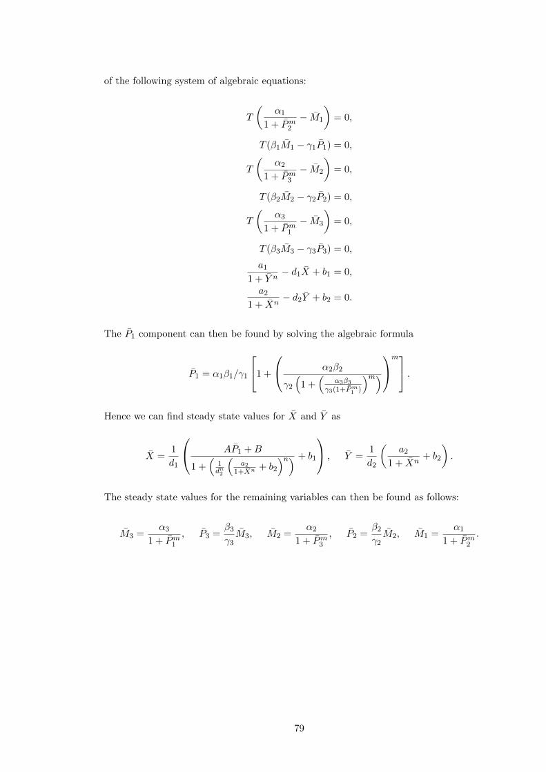
of the following system of algebraic equations:
T
(α1
1 + Pm2− M1
)= 0,
T (β1M1 − γ1P1) = 0,
T
(α2
1 + Pm3− M2
)= 0,
T (β2M2 − γ2P2) = 0,
T
(α3
1 + Pm1− M3
)= 0,
T (β3M3 − γ3P3) = 0,
a1
1 + Y n− d1X + b1 = 0,
a2
1 + Xn− d2Y + b2 = 0.
The P1 component can then be found by solving the algebraic formula
P1 = α1β1/γ1
1 +
α2β2
γ2
(1 +
(α3β3
γ3(1+Pm1 )
)m)m .
Hence we can find steady state values for X and Y as
X =1
d1
AP1 +B
1 +(
1dn2
(a2
1+Xn + b2
)n) + b1
, Y =1
d2
(a2
1 + Xn+ b2
).
The steady state values for the remaining variables can then be found as follows:
M3 =α3
1 + Pm1, P3 =
β3
γ3M3, M2 =
α2
1 + Pm3, P2 =
β2
γ2M2, M1 =
α1
1 + Pm2.
79

Figure 4.3: Effect of the coupling parameters A and B on the oscillation-induced peri-odic switch in the ODE and DDE systems, (4.1) and (4.2), respectively. (a) Oscillatorybehaviour of X in the ODE model (4.1). (b) Behaviour of X in the DDE model (4.2)with delays only in the Repressilator. Dark blue region: When B is sufficiently smalland A sufficiently large, a periodic switch is observed. Light blue region: When A and Bare small, low amplitude oscillations around the lower steady state branch are observed.Green region: When both A and B are large enough, we see low amplitude oscillationsaround the upper steady state branch. Yellow region: When A is sufficiently small and Blarge, birythmicity is observed. Parameter values: τR = 1 and τS = 0 ((b) only). T = 0.2,α1 = α2 = α3 = 100, β1 = β2 = β3 = 5, γ1 = γ2 = γ3 = 5, d1 = d2 = 1, b1 = b2 = 0,a2 = 2, m = 2, n = 4.
4.3 Analysis of the Delayed Repressilator Coupled with
Toggle Switch Model
The equation for eigenvalues λ of the linearisation near a steady state of system (4.2) has
the form
[(λ+ T )3(λ+ γ1T )(λ+ γ2T )(λ+ γ3T ) + T 6ρe−λτR
] [(λ+ d1)(λ+ d2) + σe−λτS
]= 0,
(4.4)
where τR = τm1 + τp1 + τm2 + τp2 + τm3 + τp3 and τS = τX + τY , and
ρ =α1α2α3β1β2β3m
3Pm−11 Pm−1
2 Pm−13
(1 + P1)2(1 + P2)2(1 + P3)2, σ =
−n2a2(AP1 +B)Xn−1Y n−1
(1 + Xn)2(1 + Y n)2.
In the limit τR = 0, τS = 0, the characteristic equation reduces to
[(λ+ T )3(λ+ γ1T )(λ+ γ2T )(λ+ γ3T ) + T 6ρ
][(λ+ d1)(λ+ d2) + σ] = 0, (4.5)
80

For the steady state (P1, M1, P2, M2, P3, M3, X, Y ) to be stable we require that the roots
of equation (4.5) have negative real part. We can therefore look at the polynomials in the
square brackets independently. Looking at the second bracket and expanding we have
λ2 + (d1 + d2)λ+ d1d2 + σ = 0.
The eigenvalues have negative real part provided that d1d2 + σ > 0 and d1 + d2 > 0. The
latter relation is satisfied since d1 > 0 and d2 > 0.
Now looking at the first square bracket on the left hand side of equation (4.5), we have
the equation
λ6 + a1λ5 + a2λ
4 + a3λ3 + a4λ
2 + a5λ+ a6 = 0, (4.6)
where
a1 = T (γ1 + γ2 + γ3 + 3) > 0,
a2 = T 2[γ1(γ2 + γ3 + 3) + γ2(γ3 + 3) + 3γ3 + 3] > 0,
a3 = T 3[γ1(γ2(γ3 + 3) + 3γ3 + 3) + γ2(3γ3 + 3) + 3γ3 + 1] > 0,
a4 = 3T 4[γ1(γ2(γ3 + 1) + γ3 + 1/3) + γ2(γ3 + 1/3) + (γ3/3)] > 0,
a5 = 3T 5[γ3(γ2(γ1 + 1/3) + (γ1/3)) + (γ1γ2/3)] > 0,
a6 = T 6(γ1γ2γ3 + ρ) > 0.
Then using the Routh-Hurwitz criterion, the remaining non-zero elements of the Routh
array are as follows:
b1 =a1a2 − a0a3
a1, b2 =
a1a4 − a0a5
a1, b3 = a6,
c1 =b1a3 − a1b2
b1, c2 =
b1a5 − a1b3
b1,
d1 =c1b2 − b1c2
c1, d2 = b3,
e1 =d1c2 − c1d2
d1
,
f1 = d2.
Then by the Routh-Hurwitz criterion, all roots of (4.6) have negative real part provided
81

that b1, c1, d1, e1, f1 > 0. This leads to the following result.
Lemma 4.1. Let τR = τS = 0. The steady state (P1, M1, P2, M2, P3, M3, X, Y ) of the
system (4.2) is stable whenever the conditions b1, c1, d1, e1, f1 > 0 and d1d2 +σ > 0 hold.
As in previous chapters, we assume the conditions of Lemma 4.1 hold for the remainder
of the analysis. The only way the steady state (P1, M1, P2, M2, P3, M3, X, Y ) of system
(4.2) can lose stability is if a pair of complex conjugate eigenvalues cross the imaginary
axis.
4.3.1 The Effect of Delays in the Toggle Switch
We wish to investigate whether there exists a critical time delay of τS or τR that can induce
a Hopf bifurcation resulting in sustained oscillations. Since τR and τS appear exclusively
in the first and second square brackets of (4.4), respectively, we can look at each case
independently of one another. First, we look at the case where τS > 0 and τR = 0, that
is, there are no delays in the Repressilator sub-network.
Substituting λ = iν, for real ν, into the equation
(λ+ d1)(λ+ d2) + σe−λτS = 0, (4.7)
and separating into real and imaginary parts gives
cos(ντS) =ν2 − d1d2
σ,
sin(ντS) =(d1 + d2)ν
σ.
(4.8)
Squaring and adding together we have
ν4 + (d21 + d2
2)ν2 + d21d
22 − σ2 = 0.
Let z = ν2 then we define
h(z) = z2 + (d21 + d2
2)z + d21d
22 − σ2 = 0,
82

which can be solved to give the critical frequency as
ν20 =
1
2
[−(d2
1 + d22) +
√(d2
1 + d22)2 − 4(d2
1d22 − σ2)
]. (4.9)
One should note that ν20 will only admit positive real values, provided d2
1d22 < σ2, which
implies that, for d21d
22 ≥ σ2, the roots of (4.7) have negative real parts for all values of the
time delay τS . Note that
dh(z)
dz= 2z + d2
1 + d22 > 0 for any z ≥ 0.
The critical value of the time delay τS can be found from (4.8), which gives
τS0,j =1
ν0
[arctan
((d1 + d2)ν0
ν20 − d1d2
)+ jπ
], j = 0, 1, 2, ...,
where ν0 is determined by (4.9). When τS = τS0,j , the equation (4.7) has a pair of purely
imaginary roots. In order to verify whether or not the steady state actually loses stability
at τS0,j one has to compute the sign of dRe(λ)/dτS |τS=τS0,j. Let λ(τS) = µ(τS) + iν(τS)
be the root of (4.7) near τS = τS0,j satisfying µ(τS0,j) = 0 and ν(τS0,j) = ν0. Substituting
λ = λ(τS) into (4.7) and differentiating both sides with respect to τS yields
(dλ
dτS
)−1
=(2λ+ d1 + d2)eλτS
σλ− τS
λ.
From this equation, we can find
sgn
{[d(Reλ)
dτS
]τS=τS0,j
}= sgn
Re
[(dλ
dτS
)−1]τS=τS0,j
= sgn
{Re
[(2λ+ d1 + d2)eλτS
σλ
]τS=τS0,j
}
= sgn
{2σν2
1 cos(ν1τS0) + σν1(d1 + d2) sin(ν1τS0)
σ2ν21
}.
Substituting expressions from system (4.8) gives
sgn
{[d(Reλ)
dτS
]τS=τS0,j
}=
2ν21 + d2
1 + d22
σ2=h′(ν2
1)
σ2> 0.
Hence, the roots of the equation (4.7) cross the imaginary axis at τS = τS0 , and never
83
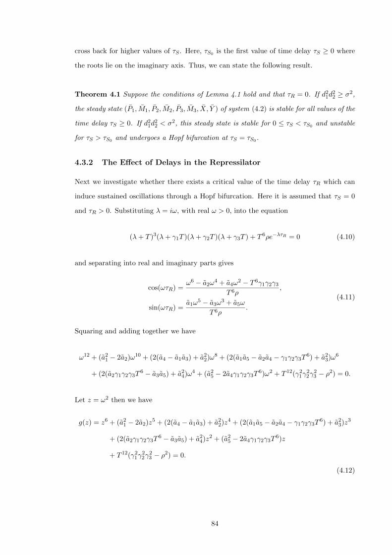
cross back for higher values of τS . Here, τS0 is the first value of time delay τS ≥ 0 where
the roots lie on the imaginary axis. Thus, we can state the following result.
Theorem 4.1 Suppose the conditions of Lemma 4.1 hold and that τR = 0. If d21d
22 ≥ σ2,
the steady state (P1, M1, P2, M2, P3, M3, X, Y ) of system (4.2) is stable for all values of the
time delay τS ≥ 0. If d21d
22 < σ2, this steady state is stable for 0 ≤ τS < τS0 and unstable
for τS > τS0 and undergoes a Hopf bifurcation at τS = τS0.
4.3.2 The Effect of Delays in the Repressilator
Next we investigate whether there exists a critical value of the time delay τR which can
induce sustained oscillations through a Hopf bifurcation. Here it is assumed that τS = 0
and τR > 0. Substituting λ = iω, with real ω > 0, into the equation
(λ+ T )3(λ+ γ1T )(λ+ γ2T )(λ+ γ3T ) + T 6ρe−λτR = 0 (4.10)
and separating into real and imaginary parts gives
cos(ωτR) =ω6 − a2ω
4 + a4ω2 − T 6γ1γ2γ3
T 6ρ,
sin(ωτR) =a1ω
5 − a3ω3 + a5ω
T 6ρ.
(4.11)
Squaring and adding together we have
ω12 + (a21 − 2a2)ω10 + (2(a4 − a1a3) + a2
2)ω8 + (2(a1a5 − a2a4 − γ1γ2γ3T6) + a2
3)ω6
+ (2(a2γ1γ2γ3T6 − a3a5) + a2
4)ω4 + (a25 − 2a4γ1γ2γ3T
6)ω2 + T 12(γ21γ
22γ
23 − ρ2) = 0.
Let z = ω2 then we have
g(z) = z6 + (a21 − 2a2)z5 + (2(a4 − a1a3) + a2
2)z4 + (2(a1a5 − a2a4 − γ1γ2γ3T6) + a2
3)z3
+ (2(a2γ1γ2γ3T6 − a3a5) + a2
4)z2 + (a25 − 2a4γ1γ2γ3T
6)z
+ T 12(γ21γ
22γ
23 − ρ2) = 0.
(4.12)
84

Without loss of generality, suppose that this equation has 6 positive real roots, denoted
by z1, z2, z3, z4, z5, z6 respectively, which would give 6 possible values of ω: ω1 =√z1,
ω2 =√z2, ω3 =
√z3, ω4 =
√z4, ω5 =
√z5, and ω6 =
√z6. With some algebraic
manipulation we obtain
τRk,j =1
ωk
[arctan
(a1ω
5k − a3ω
3k + a5ωk
ω6k − a2ω4
k + a4ω2k − T 6γ1γ2γ3
)+ jπ
], j = 0, 1, 2, ..., k = 1, 2, ..., 6.
Define
τR0 = min1≤k≤6
{τRk,0}, ω0 = ωk0 , k0 ∈ {1, 2, 3, 4, 5, 6}.
τR0 is the first value of the time delay τR > 0 where (4.10) has purely imaginary roots.
We can state the following result.
Theorem 4.2 Let τS = 0. Suppose the conditions of Lemma 4.1 hold and g′(z0) > 0,
where g(z) is defined in (4.12). Then the steady state (M1, P1, M2, P2, M3, P3, X, Y ) of
system (4.2) is stable for 0 ≤ τR < τR0 and unstable for τR > τR0 and undergoes a Hopf
bifurcation at τR = τR0.
Proof. The conclusion of Lemma 4.1 ensures the steady state (M1, P1, M2, P2, M3, P3, X, Y )
of system (4.2) is stable at τR = τS = 0 and guarantees that the roots of (4.7) have negative
real part when τS = 0. Now to prove that the steady state (M1, P1, M2, P2, M3, P3, X, Y )
loses stability at the critical time delay τR0 , let λ(τR) = µ(τR) + iω(τR) be the root of
(4.10) near τR = τR0 satisfying µ(τR0) = 0 and ω(τR0) = ω0. Substituting λ = λ(τR) into
(4.10) and differentiating with respect to τR yields
(dλ
dτR
)−1
=(6λ5 + 5a1λ
4 + 4a2λ3 + 3a3λ
2 + 2a4λ+ a5)eλτR
T 6ρλ− τR
λ.
85

From this we find
sgn
Re
[(dλ
dτR
)−1]τR=τR0
= sgn
{Re
[(6λ5 + 5a1λ
4 + 4a2λ3 + 3a3λ
2 + 2a4λ+ a5)eλτR
T 6ρλ
]τR=τR0
}
= sgn
{T 6ρ[(6ω5
0 − 4a2ω30 + 2a4ω0) cos(ω0τR0) + (5a1ω
40 − 3a3ω
20 + a5) sin(ω0τR0)]
T 12ρ2ω0
}.
Then substituting expressions from (4.11) it follows that
sgn
Re
[(dλ
dτR
)−1]τR=τR0
= sgn
{g′(ω2
0)
T 12ρ2
}> 0.
Hence, the eigenvalues of the characteristic equation cross the imaginary axis at τR = τR0 ,
thus the steady state (M1, P1, M2, P2, M3, P3, X, Y ) of system (4.2) does lose stability at
τR = τR0 . �
Using the results of Theorem 4.1 and Theorem 4.2 we obtain the following result for
the case where τR > 0 and τS > 0.
Theorem 4.3. Suppose the conditions of Lemma 4.1 hold and σ2 > d21d
22 and g′(z0) > 0,
where g(z) is defined in (4.12). Then the steady state (M1, P1, M2, P2, M3, P3, X, Y ) of
system (4.2) is stable for 0 ≤ τS < τS0 and 0 ≤ τR < τR0, and unstable for τS > τS0 or
τR > τR0, and undergoes a Hopf bifurcation at τS = τS0 or τR = τR0.
4.4 Oscillatory Behaviour of the DDE System
In previous chapters, time delays have been shown to have a significant impact on the
dynamical behaviour of GRNs when modelled using DDEs. However in past research the
effect of time delays on steady state stability has been investigated, here we wish to study
the effect of time delays on the oscillatory behaviour of a protein from the Toggle switch
sub-network in (4.2) with regards to switching and birythmicity. For the purpose of making
a comparative analysis between the ODE and DDE models, we adopt the methodology
in [139] to display our findings.
We now investigate the effects of time delays in the DDE model (4.2) on the parameter-
86

0 0.5 1 1.5A
0
2
4
6
B
(a)
0 0.1 0.2 0.3 0.4A
0
1
2
3
B
(b)
Figure 4.4: Effect of the coupling parameters A and B on the oscillation-induced periodicswitch in the DDE system (4.2) with delays only in the Toggle switch. (b) is a magnifi-cation of (a). Dark blue: When B is sufficiently small and A sufficiently large, a periodicswitch is observed. Light blue: When A and B are small, low amplitude oscillationsaround the lower steady state branch are observed. Green: When both A and B are largeenough, we see low amplitude oscillations around the upper steady state branch. Yellow:When A is sufficiently small and B large, birythmicity is observed. Orange: For small Bthere is a range of possible choices of A where, depending on initial conditions, low am-plitude oscillations around the upper steady state branch or periodic switch is observed.Pink: For small B if A is sufficiently small and within a certain range, depending on initialconditions, low amplitude oscillations around the lower steady state branch or periodicswitch is observed. Parameter values: τR = 0, τS = 40, T = 0.2, α1 = α2 = α3 = 100,β1 = β2 = β3 = 5, γ1 = γ2 = γ3 = 5, d1 = d2 = 1, b1 = b2 = 0, a2 = 2, m = 2, n = 4.
dependent periodic switch and general system behaviour. Firstly it should be noted that
with regards to stability of steady states, the individual time delays were not important.
What’s important, is the combined time delay of the Toggle switch and likewise the com-
bined time delay of the Repressilator, i.e. the sum of the individual time delays present
in each respective sub-network. This is also the case with regards to the effect of time
delays on the system behaviour after oscillations are induced. Therefore, we denote the
combined time delay in the Repressilator as τR = τm1 + τp1 + τm2 + τp2 + τm3 + τp3 , and
the combined delay in the Toggle switch as τS = τX + τY .
In Figure 4.3(b) the combined time delay in the Repressilator is increased to τR = 1,
whilst the time delay in the Toggle switch is kept as τS = 0. The presence of delays in
the Repressilator simply makes the upright boundary line shift slightly to the left, whilst
the point of intersection of this line and the vertical axis remains at B = 6.8. It therefore
requires a smaller coupling amplitude to induce birythmicity. Overall, the time delays
from the Repressilator have little effect on the oscillatory dynamics of X in the Toggle
87

0 5 10 15a
1
0
5
10
15
X
(a)
800 900 1000time t
0
5
10
15
X,Y
(b)
XY
0 2 4 6 8a
1
0
1
2
3
X
(c)
800 900 1000 1100time t
0
1
2
X,Y
(d)XY
0 5 10 15a
1
0
5
10
15
X
(e)
800 900 1000time t
0
5
10
15
X,Y
(f)
XY
0 2 4 6 8a
1
0
2
4
X
(g)
800 900 1000 1100time t
0
2
4
X,Y
(h)X (from CI1)Y (from CI1)X (from CI2)Y (from CI2)
Figure 4.5: Oscillatory behaviour in the DDE model (4.2). (a) Bifurcation diagram ofvariable X as a function of parameter a1. The blue curve shows that this variable switchesbetween the lower and upper steady states, with different dynamics than seen in theODE model (4.1). (b) Time evolutions of X and Y . (c) When amplitude of couplingis insufficient, a periodic switch cannot be induced and variable X oscillates around thelower steady state. (d) Corresponding time evolution of X and Y . (e) When amplitude ofcoupling is high, oscillations around the upper steady state can occur. (f) Correspondingtime evolution of X and Y . (g) When amplitude of coupling is very low, oscillationsof the Repressilator can induce birythmicity. (h) Corresponding evolutions of X and Y .Parameter values: τR = 0, τS = 40, T = 0.2, α1 = α2 = α3 = 100, β1 = β2 = β3 = 5,γ1 = γ2 = γ3 = 5, d1 = d2 = 1, b1 = b2 = 0, a2 = 2, m = 2, n = 4. Coupling parameters:A = 0.3, B = 0.5 ((a) and (b)), A = 0.05, B = 0.5 ((c) and (d)), A = 0.3, B = 2.5((e) and (f)), A = 0.05, B = 2.5 ((g) and (h)). For the latter case, initial conditions areX(0) = 0.1 and Y (0) = 10 (denoted by CI1), leading to the lower limit cycle or X(0) = 10and Y (0) = 0.1 (denoted by CI2), leading to the upper limit cycle.
88

0 5 10 15a
1
0
5
10
15
X
(a)
1600 1700 1800time t
0
5
10
15
X,Y
(b)X (from CI1)Y (from CI1)X (from CI2)Y (from CI2)
0 2 4 6 8a
1
0
2
4
6
8
X
(c)
1600 1700 1800time t
0
2
4
6
X,Y
(d)X (from CI1)Y (from CI1)X (from CI2)Y (from CI2)
Figure 4.6: New Oscillatory behaviour found in the DDE model (4.2). (a) For sufficientlylarge amplitude of coupling, it is possible to induce a phenomenon where, depending oninitial conditions, variable X can undergo small-amplitude oscillations around the uppersteady state or undergo a periodic switch. (b) Time evolution of corresponding X and Y .(c) For a sufficiently small amplitude of coupling, a type of behaviour is possible where,depending on initial conditions, variable X can undergo a periodic switch or undergo small-amplitude oscillations around the lower steady state. (d) Corresponding time evolutionof X and Y . Parameter values: τR = 0, τS = 40, T = 0.2, α1 = α2 = α3 = 100,β1 = β2 = β3 = 5, γ1 = γ2 = γ3 = 5, d1 = d2 = 1, b1 = b2 = 0, a2 = 2, m = 2, n = 4.Coupling parameters: A = 0.3, B = 1.25 ((a) and (b)), A = 0.12, B = 1 ((c) and (d)).Initial conditions are X(0) = 0.1 and Y (0) = 10 (denoted by CI1), or X(0) = 10 andY (0) = 0.1 (denoted by CI2).
switch. With this in mind we now ignore the presence of time delays in the Repressilator
and investigate the effects of time delays in the Toggle switch.
The types of oscillatory behaviour that can occur as a result of delays in the Toggle
switch is summarized in Figure 4.4. The same four behaviours of periodic switching, lower
oscillations, upper oscillations, and birythmicity are still present in the DDE system as
appeared in the ODE model. Interestingly, the inclusion of these time delays in the Toggle
switch has given rise to new behaviours as well, unseen in the ODE model. The dynamics
89

of X remain the same for choices of A and B which lie in the light blue region (lower
oscillations), green region (upper oscillations), and yellow region (birythmicity). However,
in the dark blue region a periodic switch is still induced in X although the dynamical
behaviour is drastically different, shown in Figure 4.5(a) and (b). The solution for X
begins to oscillate around the upper steady state branch but as a1 becomes very small X
switches for a short time to the lower branch before switching back to the upper branch.
More importantly, the new behaviour that occurs due to the inclusion of time delays in
the Toggle switch is seen in the orange and pink regions of Figure 4.4. When the coupling
parameter B is small and amplitude of coupling A is sufficiently large such that it lies in
the orange region, a phenomenon is induced whereby, depending on the initial conditions,
X will either oscillate around the upper steady state branch or undergo a periodic switch.
These dynamics are depicted in Figure 4.6(a) and (b). Similarly, another new type of
behaviour is observed in the pink region of Figure 4.4 where, depending on the initial
conditions, X will either oscillate around the lower steady state branch or undergo a
periodic switch. These dynamics are illustrated in Figure 4.6(c) and (d).
The bifurcation and solution diagrams shown here reveal new types of behaviour that
could not be possible in the network described by the ODE model (4.1). If we look at the
periodic switch observed in Figure 4.2(a) and (b) we see that in the model without delays
the solution of X stays near the lower steady state branch for a long time before passing
the second saddle node, where it then goes to the upper branch. X only stays along the
upper branch for a short time before switching to the lower branch again. Conversely, if
we look at the periodic switch observed in the DDE model, in Figure 4.5(a) and (b), we
see that X does not move far along the lower steady state branch. The dynamics also
contrast in that more time is spent along the upper branch, shown in Figure 4.5(b), than
in the ODE model.
We see that the time delays associated with the two parts of the network, namely, the
Repressilator and Toggle switch need to be treated separately. Compared to the behaviours
seen in Figure 4.3(a), the plot in Figure 4.3(b) reveals very little change. Overall, the
inclusion of delays in the Repressilator doesn’t produce a dramatic difference in dynamics
of X.
The final comparison that can be made between the results of the DDE model and
those found by Gonze [139] is the appearance of two new oscillatory dynamics. Figure 4.4
90

gives rise to parameter regions where X is capable of undergoing a periodic switch and
either upper or lower oscillations depending on initial conditions. The new behaviours
that appear as a result of the delays in the Toggle switch are not limited to this, other
forms of spiking dynamics in the oscillations of X can also be observed (not shown here).
It is evident that in modelling systems where non-negligible time delays exist, such as in
GRNs, careful consideration of these delays can help unravel new information that may
have otherwise been lost.
4.5 Discussion
In this chapter we have discussed a mathematical model for the analysis of a GRN com-
prised of the Repressilator [74] coupled with the Toggle switch [80] where one protein in
the Toggle switch is under the control of one protein in the Repressilator in a master/slave
setup. We have focussed on the role of transcriptional and translational time delays on
the dynamics of the coupled GRN. Our analysis extends an ealier result of Gonze [139]
by introducing time delays into the system, where we were able to find new dynamical
behaviours that were not possible in the absence of the time delays. Numerical simulations
have allowed us to observe these new behaviours and make direct comparisons with the
earlier results.
The results in this chapter show that although it may be difficult to control values of
coupling parameters in practice, other parameters in the oscillator itself could be altered
to produce the desired amplitude of oscillations. Likewise, time delays would also be
difficult to alter however understanding the potential effects that time delays can have on
the system dynamics could indeed help to provide greater control over parameter tuning
in an artificial and experimental environment.
91

Chapter 5
Discussion and Future Work
5.1 Summary and Conclusions
Research into mathematical models of genetic regulatory networks has provided great
insight into the behaviour and development of key life processes in an organism, in a
quantitative as well as qualitative way. Correct mathematical representation of real bio-
logical systems is vital to achieve a more complete picture of the mechanisms at work in
the biological environment. Inclusion of time delays into these models can help unravel
the causes of certain phenomena such as Hopf bifurcations and help understand their
biological implications.
This thesis examined the effects of time delays in systems describing the dynamics of
genetic regulatory networks. In a real biological setting, these delays are associated with
the transcription and translation processes during gene expression and, due to the relative
time scales of the intrinsic processes, are non-negligible and therefore need to be properly
accounted for. We have considered three different GRN network motifs, each with its own
forms of regulation between genes. Delay differential equations have been used to describe
each model and comparisons have been made with the equivalent ODE description.
The first model focused on the role of transcriptional and translational time delays in
an activation-inhibition GRN, and discussed the relevance of behaviour in such models to
the onset and development of certain types of cancer. The analysis provided analytical ex-
pressions of steady states and showed conditions for the occurrence of periodic oscillations
due to the time delays. The results from numerical simulations illustrated the presence
92

of new oscillatory behaviour in the simplified delayed model, with fast mRNA dynamics,
which could not be seen in the existing ODE model in the literature. It also showed the
relationships between various system parameters and the time delays, and their effect on
steady state stability.
The second model focused on the role of transcriptional and translational time delays
in a three-gene network where each gene inhibits the expression of the next gene in the
cycle, whilst promoting the expression of itself. It was shown that although the literature
suggests that oscillations cannot exist in a Repressilator model with a small Hill coefficient,
the inclusion of auto-activation and asymmetry could in fact give rise to oscillations. The
results of the analysis showed that only one of the steady states has the potential to lose
stability through parameter variations, and that the presence of multiple delays can lead
to periodic switching of stability for this steady state. The switching between stability
of the other steady states was representative of cell fate decisions in the immune system,
which showed the importance of parameter tuning on the long term system behaviour.
The third model focused on the effect of transcriptional and translational time delays
on the Repressilator model coupled with a Toggle switch. This was done by making a
comparative analysis between the DDE model and an ODE model from earlier literature.
Steady state stability analysis was performed to provide analytical conditions for the
occurrence of oscillations due to time delays, and numerical simulations were used to
study the effect of the delays on the different types of oscillations that can be exhibited
by one of the system proteins. The results suggest that with regards to both stability and
behaviour of oscillations, it is the combined delays of each respective sub-network that has
an impact on the system dynamics, rather than the individual delays. It was found that
the delays in the Repressilator have little effect on the dynamics of the observed protein in
the Toggle switch, however the delays in the Toggle switch lead to new types of oscillatory
behaviour, which were impossible in the ODE system. These results stress the importance
of transcriptional and translational time delays in not only steady state stability, but also
the system behaviour once oscillations have been induced.
The outcomes of this thesis stress the significance of time delays within GRNs. With-
out careful consideration of delays, it may be likely that one could miss vital information
surrounding the genetic model; whether it be oscillations induced by delay dependent
Hopf bifurcations, or rich dynamical patterns which exist only in a delayed model setting.
93
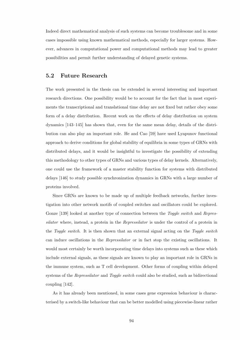
Indeed direct mathematical analysis of such systems can become troublesome and in some
cases impossible using known mathematical methods, especially for larger systems. How-
ever, advances in computational power and computational methods may lead to greater
possibilities and permit further understanding of delayed genetic systems.
5.2 Future Research
The work presented in the thesis can be extended in several interesting and important
research directions. One possibility would be to account for the fact that in most experi-
ments the transcriptional and translational time delay are not fixed but rather obey some
form of a delay distribution. Recent work on the effects of delay distribution on system
dynamics [143–145] has shown that, even for the same mean delay, details of the distri-
bution can also play an important role. He and Cao [59] have used Lyapunov functional
approach to derive conditions for global stability of equilibria in some types of GRNs with
distributed delays, and it would be insightful to investigate the possibility of extending
this methodology to other types of GRNs and various types of delay kernels. Alternatively,
one could use the framework of a master stability function for systems with distributed
delays [146] to study possible synchronization dynamics in GRNs with a large number of
proteins involved.
Since GRNs are known to be made up of multiple feedback networks, further inves-
tigation into other network motifs of coupled switches and oscillators could be explored.
Gonze [139] looked at another type of connection between the Toggle switch and Repres-
silator where, instead, a protein in the Repressilator is under the control of a protein in
the Toggle switch. It is then shown that an external signal acting on the Toggle switch
can induce oscillations in the Repressilator or in fact stop the existing oscillations. It
would most certainly be worth incorporating time delays into systems such as these which
include external signals, as these signals are known to play an important role in GRNs in
the immune system, such as T cell development. Other forms of coupling within delayed
systems of the Repressilator and Toggle switch could also be studied, such as bidirectional
coupling [142].
As it has already been mentioned, in some cases gene expression behaviour is charac-
terised by a switch-like behaviour that can be better modelled using piecewise-linear rather
94

than continuous transcription functions [38, 41]. Whilst some preliminary work has been
done recently on the analysis of piecewise-linear systems with discrete time delays, pri-
marily in engineering applications [147–149], the dynamics of GRNs with piecewise-linear
transcription functions and transcriptional/translational delays have remained completely
unexplored. Further inclusion of distributed delays would make such models mathemati-
cally very challenging, but it could provide a new level of understanding of GRN dynamics.
95
Bibliography
[1] U. Alon, An Introduction to Systems Biology, Champan & Hall, Boca Raton, USA,
2007.
[2] H. de Jong, “Modeling and simulation of genetic regulatory systems: a literature
review,” Journal of Computational Biology, vol. 9, no. 1, pp. 67-103, 2002.
[3] G. Bernot, J.-P. Comet, A. Richard, M. Chaves, J.-L. Gouze, and R. Dayan, “Model-
ing and analysis of gene regulatory networks,” in Modeling in Computational Biology
and Biomedicine, F. Cazals and P. Kornprobst, Eds., pp. 47-80, Springer, Berlin,
Germany, 2013.
[4] D. Endy and R. Brent, “Modelling cellular behaviour,” Nature, vol. 409, no. 6818,
pp. 391-395, 2001.
[5] J. Hasty, D. McMillen, F. Isaacs, and J.J. Collins, “Computational studies of gene
regulatory networks: in numero molecular biology,” Nature Reviews Genetics, vol. 2,
no. 4, pp. 268-279, 2001.
[6] A. Tusek and Z. Kurtanjek, “Mathematical modelling of gene regulatory networks,”
in Applied Biological Engineering—Principles and Practice, chapter 5, InTech, Rijeka,
Croatia, 2012.
[7] M. Hecker, S. Lambeck, S. Toepfer, E. van Someren, and R. Guthke, “Gene regulatory
network inference: data integration in dynamic models—a review,” BioSystems, vol.
69, no. 1, pp. 86-103, 2009.
[8] S. A. Kauffman, “Metabolic stability and epigenesis in randomly constructed genetic
nets,” Journal of Theoretical Biology, vol. 22, no. 3, pp. 437-467, 1969.
96
[9] R. Thomas, “Boolean formalization of genetic control circuits,” Journal of Theoretical
Biology, vol. 42, no. 3, pp. 563-585, 1973.
[10] R. Somogyi and C. A. Sniegoski, “Modeling the complexity of genetic networks: un-
derstanding multigenic and pleiotropic regulation,” Complexity, vol. 1, no. 6, pp.
45-63, 1996.
[11] R. Albert, “Boolean modelling of genetic regulatory networks,” in Complex Networks,
vol. 650 of Lecture Notes in Physics, pp. 459-481, Springer, Berlin, Germany, 2004.
[12] P. Smolen, D. A. Baxter, and J. H. Byrne, “Modeling transcriptional control in gene
networks—methods, recent results, and future directions,” Bulletin of Mathematical
Biology, vol. 62, no. 2, pp. 247-292, 2000.
[13] I. Shmulevich, E. R. Dougherty, and W. Zhang, “From Boolean to probabilistic
Boolean networks as models of genetic regulatory networks,” Proceedings of the IEEE,
vol. 90, no. 11, pp. 1778-1792, 2002.
[14] A. Silvescu and V. Honavar, “Temporal Boolean network models of genetic networks
and their inference from gene expression time series,” Complex Systems, vol. 13, no.
1, pp. 61-78, 2001.
[15] M. Davidich and S. Bornholdt, “The transition from differential equations to Boolean
networks: a case study in simplifying a regulatory network model,” Journal of The-
oretical Biology, vol. 255, no. 3, pp. 269-277, 2008.
[16] R. Xu, G.K. Venayagamoorthy, and D.C. Wunsch II, “Modeling of gene regulatory
networks with hybrid differential evolution and particle swarm optimization,” Neural
Networks, vol. 20, no. 8, pp. 917-927, 2007.
[17] F. Karlsson and M. Hornquist, “Order or chaos in Boolean gene networks depends
on the mean fraction of canalizing functions,” Physica A, vol. 384, no. 2, pp. 747-757,
2007.
[18] G. N. Brock, V. Pihur, and L. Kubatko, “Detecting gene regulatory networks from
microarray data using fuzzy logic,” in Fuzzy Systems in Bioinformatics and Compu-
tational Biology, Y. Jin and L. Wang, Eds., vol. 242 of Studies in Fuzziness and Soft
Computing, pp. 141-163, Springer, Berlin, Germany, 2009.
97

[19] P. J. Woolf and Y. Wang, “A fuzzy logic approach to analyzing gene expression data,”
Physiological Genomics, vol. 3, no. 1, pp. 9-15, 2000.
[20] L. G. Volkert and N. Malhis, “An efficient method for fuzzy identification of regulatory
events in gene expression time series data,” in Proceedings of the IEEE Symposium
on Computational Intelligence in Bioinformatics and Computational Biology (CIBCB
’04), pp. 17-24, IEEE, La Jolla, Claif, USA, October 2004.
[21] P. Das, P. Rakshit, A. Konar, M. Nasipuri, and A. K. Nagar, “Fuzzy relational system
for identification of gene regulatory network,” in Proceedings of the World Congress in
Computer Science, Computer Engineering, and Applied Computing (WORLDCOMP
’09), Las Vegas, Nev, USA, July 2009.
[22] T. A. Al Qazlan, A. Hamdi-Cherif, and C. Kara-Mohamed, “State of the art of fuzzy
methods for gene regulatory networks inference,” The Scientific World Journal, vol.
2015, Article ID 148010, 11 pages, 2015.
[23] B. C. Goodwin, Temporal Organization in Cells, Academic Press, New York, NY,
USA, 1963.
[24] B. C. Goodwin, “Oscillatory behavior in enzymatic control processes,” in Advances
in Enzyme Regulation, G. Weber, Ed., pp. 425-438, Pergamon Press, Oxford, UK,
1965.
[25] J.-L. Gouze, “Positive and negative circuits in dynamical systems,” Journal of Bio-
logical Systems, vol. 6, no. 1, pp. 11-15, 1998.
[26] E.H. Snoussi, “Necessary conditions for multistationarity and stable periodicity,”
Journal of Biological Systems, vol. 6, no. 1, pp. 3-9, 1998.
[27] J. J. Tyson and H.G. Othmer, “The dynamics of feedback control circuits in biochem-
ical pathways,” Progress in Theoretical Biology, vol. 5, pp. 1-62, 1978.
[28] A. D. Keller, “Specifying epigenetic states with autoregulatory transcription factors,”
Journal of Theoretical Biology, vol. 170, no. 2, pp. 175-181, 1994.
[29] R. Heinrich and S. Schuster, The Regulation of Cellular Systems, Chapman & Hall,
New York, NY, USA, 1996.
98
[30] J. L. Cherry and F. R. Adler, “How to make a biological switch,” Journal of Theo-
retical Biology, vol. 203, no. 2, pp. 117-133, 2000.
[31] G. Yagil, “Quantitative aspects of protein induction,” Current Topics in Cellular
Regulation, vol. 9, pp. 183-235, 1975.
[32] A. Polynikis, S. J. Hogan, and M. di Bernado, “Comparing different ODE modelling
approaches for gene regulatory networks,” Journal of Theoretical Biology, vol. 261,
no. 4, pp. 511-530, 2009.
[33] S. Widder, J. Schicho, and P. Schuster, “Dynamic patterns of gene regulation. I.
Simple two-gene systems,” Journal of Theoretical Biology, vol. 246, no. 3, pp. 395-
419, 2007.
[34] S. Goutelle, M. Maurin, F. Rougier et al., “The Hill equation: a review of its capa-
bilities in pharmacological modelling,” Fundamental and Clinical Pharmacology, vol.
22, no. 6, pp. 633-648, 2008.
[35] J. N. Weiss, “The Hill equation revisited: uses and misuses,” The FASEB Journal,
vol. 11, no. 11, pp. 835-841, 1997.
[36] M. Santillan, “On the use of the Hill functions in mathematical models of gene reg-
ulatory networks,” Mathematical Modelling of Natural Phenomena, vol. 3, no. 2, pp.
85-97, 2008.
[37] L. Glass and S. A. Kauffman, “The logical analysis of continuous, non-linear biochem-
ical control networks,” Journal of Theoretical Biology, vol. 39, no. 1, pp. 103-129,
1973.
[38] L. Glass, “Classification of biological networks by their qualitative dynamics,” Journal
of Theoretical Biology, vol. 54, no. 1, pp. 85-107, 1975.
[39] E. Plahte, T. Mestl, and S. W. Omholt, “A methodological basis for description and
analysis of systems with complex switch-like interactions,” Journal of Mathematical
Biology, vol. 36, no. 4, pp. 321-348, 1998.
[40] E. Plahte and S. Kjøglum, “Analysis and generic properties of gene regulatory net-
works with graded response functions,” Physica D, vol. 201, no. 1-2, pp. 150-176,
2005.
99
[41] R. Casey, H. de Jong, and J.-L. Gouze, “Piecewise-linear models of genetic regulatory
networks: equilibria and their stability,” Journal of Mathematical Biology, vol. 52, no.
1, pp. 27-56, 2006.
[42] J. Gebert, N. Radde, and G.-W. Weber, “Modeling gene regulatory networks with
piecewise linear differential equations,” European Journal of Operational Research,
vol. 181, no. 3, pp. 1148-1165, 2007.
[43] E. Plahte, T. Mestl, and S. W. Omholt, “Global analysis of steady points for sys-
tems of differential equations with sigmoid interactions,” Dynamics and Stability of
Systems, vol. 9, no. 4, pp. 275-291, 1994.
[44] H. El Snoussi and R. Thomas, “Logical identification of all steady states: the concept
of feedback loop characteristic states,” Bulletin of Mathematical Biology, vol. 55, no.
5, pp. 973-991, 1993.
[45] A. Hoffmann, A. Levchenko, M. L. Scott, and D. Baltimore, “The IκB-NF-κB sig-
naling module: temporal control and selective gene activation,” Science, vol. 298, no.
5596, pp. 1241-1245, 2002.
[46] S. L. Werner, D. Barken, and A. Hoffmann, “Stimulus specificity of gene expression
programs determined by temporal control of IKK activity,” Science, vol. 309, no.
5742, pp. 1857-1861, 2005.
[47] N. Geva-Zatorsky, N. Rosenfeld, S. Itzkovitz et al., “Oscillations and variability in
the p53 system,” Molecular Systems Biology, vol. 2, no. 1, Article ID 2006.0033, 2006.
[48] L. Ma, J. Wagner, J. J. Rice, W. Hu, A. J. Levine, and G. A. Stolovitzky, “A plausible
model for the digital response of p53 to DNA damage,” Proceedings of the National
Academy of Sciences of the United States of America, vol. 102, no. 40, pp. 14266-
14271, 2005.
[49] B. T. Hennessy, D. L. Smith, P. T. Ram, Y. Lu, and G. B. Mills, “Exploiting the
PI3K/AKT pathway for cancer drug discovery,” Nature Reviews Drug Discovery, vol.
4, no. 12, pp. 988-1004, 2005.
100

[50] T. M. K. Cheng, S. Gulati, R. Agius, and P. A. Bates, “Understanding cancer mech-
anisms through network dynamics,” Briefings in Functional Genomics, vol. 11, no. 6,
Article ID els025, pp. 543-560, 2012.
[51] L. B. Edelman, J. A. Eddy, and N. D. Price, “In silico models of cancer,” Wiley
Interdisciplinary Reviews: Systems Biology and Medicine, vol. 2, no.4, pp. 438-459,
2010.
[52] N. A. M. Monk, “Oscillatory expression of Hes1, p53, and NF-κB driven by tran-
scriptional time delays,” Current Biology, vol. 13, no. 16, pp. 1409-1413, 2003.
[53] A. Wan and X. Zou, “Hopf bifurcation analysis for a model of genetic regulatory
system with delay,” Journal of Mathematical Analysis and Applications, vol. 356, no.
2, pp. 464-476, 2009.
[54] K. Wang, L. Wang, Z. Teng, and H. Jiang, “Stability and bifurcation of genetic
regulatory networks with delays,” Neurocomputing, vol. 73, no. 16-18, pp. 2882-2892,
2010.
[55] M. Bodnar, U. Forys, and J. Poleszczuk, “Analysis of biochemical reactions models
with delays,” Journal of Mathematical Analysis and Applications, vol. 376, no. 1, pp.
74-83, 2011.
[56] Z. Wang, Z. Liu, and R. Yuan, “Stability and bifurcation in a gene regulatory network
model with delay,” Zeitschrift fur Angewandte Mathematik und Mechanik, vol. 92, no.
4, pp. 290-303, 2012.
[57] M. Xiao, W. X. Zheng, and J. Cao, “Stability and bifurcation of genetic regulatory
networks with small RNAs and multiple delays,” International Journal of Computer
Mathematics, vol. 91, no. 5, pp. 907-927, 2014.
[58] M. Xiao and J. Cao, “Genetic oscillation deduced from Hopf bifurcation in a genetic
regulatory network with delays,” Mathematical Biosciences, vol. 215, no. 1, pp. 55-63,
2008.
[59] W. He and J. Cao, “Robust stability of genetic regulatory networks with distributed
delay,” Cognitive Neurodynamics, vol. 2, no. 4, pp. 355-361, 2008.
101
[60] B. D. Aguda, Y. Kim, M. G. Piper-Hunter, A. Friedman, and C. B. Marsh, “Mi-
croRNA regulation of a cancer network: consequences of the feedback loops involving
miR-17-92, E2F, and Myc,” Proceedings of the National Academy of Sciences of the
United States of America, vol. 105, no. 50, pp. 19678-19683, 2008.
[61] B. D. Aguda, “Modeling microRNA-transcription factor networks in cancer,” in Mi-
croRNA Cancer Regulation: Advanced Concepts, Bioinformatics and Systems Biology
Tools, U. Schmitz, O. Wolkenhauer, and J. Vera, Eds., vol. 774 of Advances in Exper-
imental Medicine and Biology, pp. 149-167, Springer, Dordrecht, The Netherlands,
2013.
[62] A. S. Ribeiro, J. J. Grefenstette, and S. A. Kauffman, “Modeling gene regulatory
networks with delayed stochastic dynamics,” in Handbook of Research on Computa-
tional Methodologies in Gene Regulatory Networks, S. Das, D. Caragea, S. M. Welch,
and W. H. Hsu, Eds., pp 198-218, Medical Information Science Reference, New York,
NY, USA, 2010.
[63] N. MacDonald, “Time lag in a model of a biochemical reaction sequence with end
product inhibition,” Journal of Theoretical Biology, vol. 67, no. 3, pp. 549-556, 1977.
[64] I. R. Epstein and Y. Luo, “Differential delay equations in chemical kinetics. Nonlin-
ear models: the cross-shaped phase diagram and the Oregonator,” The Journal of
Chemical Physics, vol. 95, no. 1, pp. 244-254, 1991.
[65] J. Paulsson, “Models of stochastic gene expression,” Physics of Life Reviews, vol. 2,
no. 2, pp. 157-175, 2005.
[66] S. Rosenfeld, “Stochastic cooperativity in non-linear dynamics of gene regulatory
networks,” Mathematical Biosciences, vol. 210, no. 1, pp. 121-142, 2007.
[67] A. Raj and A. van Oudenaarden, “Nature, nurture, or chance: stochastic gene ex-
pression and its consequences,” Cell, vol. 135, no. 2, pp. 216-226, 2008.
[68] P. S. Swain, M. B. Elowitz, and E. D. Siggia, “Intrinsic and extrinsic contributions
to stochasticity in gene expression,” Proceedings of the National Academy of Sciences
of the United States of America, vol. 99, no. 20, pp. 12795-12800, 2002.
102

[69] K. M. Herbert, A. La Porta, B. J. Wong et al., “Sequence resolved detection of pausing
by single RNA polymerase molecules,” Cell, vol. 125, no. 6, pp. 1083-1094, 2006.
[70] A. S. Ribeiro, O.-P. Smolander, T. Rajala, A. Hakkinen, and O. Yli-Harja, “Delayed
stochastic model of transcription at the single nucleotide level,” Journal of Compu-
tational Biology, vol. 16, no. 4, pp. 539-553, 2009.
[71] M. Voliotis, N. Cohen, C. Molina-Parıs, and T. B. Liverpool, “Fluctuations, pauses
and backtracking in DNA transcription,” Biophysical Journal, vol. 94, no. 2, pp.
334-348, 2008.
[72] A. S. Ribeiro, “Stochastic and delayed stochastic models of gene expression and reg-
ulation,” Mathematical Biosciences, vol. 223, no. 1, pp. 1-11, 2010.
[73] M. J. Dunlop, R. S. Cox III, J. H. Levine, R. M. Murray, and M. B. Elowitz, “Reg-
ulatory activity revealed by dynamic correlations in gene expression noise,” Nature
Genetics, vol. 40, no. 12, pp. 1493-1498, 2008.
[74] M. B. Elowitz and S. Leibler, “A synthetic oscillatory network of transcriptional
regulators,” Nature, vol. 403, no. 6767, pp. 335-338, 2000.
[75] M. B. Elowitz, A. J. Levine, E. D. Siggia, and P. S. Swain, “Stochastic gene expression
in a single cell,” Science, vol. 297, no. 5584, pp. 1183-1186, 2002.
[76] S. Rosenfeld, “Stochastic oscillations in genetic regulatory networks: application to
microarray experiments,” Eurasip Journal on Bioinformatics and Systems Biology,
vol. 2006, Article ID 59526, 2006.
[77] M. Kærn, T. C. Elston, W. J. Blake, and J. J. Collins, “Stochasticity in gene ex-
pression: from theories to phenotypes,” Nature Reviews Genetics, vol. 6, no. 6, pp.
451-464, 2005.
[78] D. Bratsun, D. Volfson, L. S. Tsimring, and J. Hasty, “Delay-induced stochastic
oscillations in gene regulations,” Proceedings of the National Academy of Sciences of
the United States of America, vol. 102, no. 41, pp. 14593-14598, 2005.
[79] E. Zavala and T. T. Marquez-Lago, “Delays induce novel stochastic effects in negative
feedback gene circuits,” Biophysical Journal, vol. 106, no. 2, pp. 467-478, 2014.
103

[80] T. S. Gardner, C. R. Cantor, and J. J. Collins, “Construction of a genetic toggle
switch in Escherichia coli,” Nature, vol. 403, no. 6767, pp. 339-342, 2000.
[81] H. El Samad, M. Khammash, L. Petzold, and D. Gillespie, “Stochastic modelling of
gene regulatory networks,” International Journal of Robust and Nonlinear Control,
vol. 15, no. 15, pp. 691-711, 2005.
[82] M. Barrio, K. Burrage, A. Leier, and T. Tian, “Oscillatory regulation of Hes1: discrete
stochastic delay modelling and simulation,” PLoS Computational Biology, vol. 2, no.
9, article e117, 2006.
[83] X. Cai, “Exact stochastic simulation of coupled chemical reactions with delays,” Jour-
nal of Chemical Physics, vol. 126, Article ID 124108, 2007.
[84] M. Jansen and P. Pfaffelhuber, “Stochastic gene expression with delay,” Journal of
Theoretical Biology, vol. 364, pp. 355-363, 2015.
[85] N. Friedman, M. Linial, I. Nachman, and D. Peer, “Using Bayesian networks to
analyze expression data,” Journal of Computational Biology, vol. 7, no. 3-4, pp. 601-
620, 2000.
[86] D. Heckerman, “A tutorial on learning with Bayesian networks,” Microsoft Research
Technical Report MSR-TR-95-06, 1996.
[87] A. V. Werhli and D. Husmeier, “Reconstructing gene regulatory networks with
Bayesian networks by combining expression data with multiple sources of prior knowl-
edge,” Statistical Applications in Genetics and Molecular Biology, vol. 6, article 15,
2007.
[88] P. T. Spellman, G. Sherlock, M. Q. Zhang et al., “Comprehensive identification of cell
cycle-regulated genes of the yeast Saccharomyces cerevisiae by microarray hybridiza-
tion,” Molecular Biology of the Cell, vol. 9, no. 12, pp. 3273-3297, 1998.
[89] J. M. Heffernan and R. M. Corless, “Solving some delay differential equations with
computer algebra,” Applied Probability Trust, 2005.
[90] W. Michiels and S. Niculescu, Stability, control, and computation for time-delay sys-
tems: An eigenvalue-based approach, SIAM, Philadelphia, 2014.
104

[91] T. Erneaux, Applied Delay Differential Equations, Springer, New York, NY, USA,
2009.
[92] J. Lewis, “Autoinhibition with transcriptional delay: a simple mechanism for the
zebrafish somitogenesis oscillator,” Current Biology, vol. 13, pp. 1398-1408, 2003.
[93] Y. N. Kyrychko and K. B. Blyuss, “Global properties of a delayed SIR model with
temporary immunity and nonlinear incidence rate,” Nonlinear Analysis Real World
Applications, vol. 6, no. 3, pp. 495-507, 2005.
[94] G. Danaei, S. Vander Hoorn, A.D Lopez, C.J.L. Murray, and M. Ezzati, “Causes of
cancer in the world: comparative risk assessment of nine behavioural and environ-
mental risk factors,” The Lancet, vol. 366, no. 9499, pp. 1784-1793, 2005.
[95] M. Boshart, L. Gissmann, H. Ikenberg, A. Kleinheinz, W. Scheurlen, and H. zur
Hausen, “A new type of papillomavirus DNA, its presence in genital cancer biopsies
and in cell lines derived from cervical cancer,” The EMBO Journal, vol. 3, no. 5, pp.
1151-1157, 1984.
[96] D.F. Easton, “How many more breast cancer predisposition genes are there?” Breast
Cancer Research, vol. 1, no. 1, pp. 14-17, 1999.
[97] G. Thomas, K.B. Jacobs, M. Yeager et al., “Multiple loci identified in a genome-wide
association study of prostate cancer,” Nature Genetics, vol. 40, no. 3, pp. 310-315,
2008.
[98] B.M. Wolpin, C. Rizzato, P. Kraft et al., “Genome-wide association study identifies
multiple susceptibility loci for pancreatic cancer,” Nature Genetics, vol. 46, no. 9, pp.
994-1000, 2014.
[99] H.-Y. Yeh, S.-W. Cheng, Y.-C. Lin, C.-Y. Yeh, S.-F. Lin, and V.-W. Soo, “Identifying
significant genetic regulatory networks in the prostate cancer from microarray data
based on transcription factor analysis and conditional independency,” BMC Medical
Genomics, vol. 2, article 70, 2009.
[100] E. Bonnet, T. Michoel, and Y. Van de Peer, “Prediction of a gene regulatory net-
work linked to prostate cancer from gene expression, microRNA and clinical data,”
Bioinformatics, vol. 26, no. 18, Article ID btq395, pp. i638-i644, 2010.
105
[101] X. Wang and O. Gotoh, “Inference of cancer-specific gene regulatory networks using
soft computing rules,” Gene Regulation and Systems Biology, vol. 2010, no. 4, pp.
19-34, 2010.
[102] S. Vineetha, C. Chandra Shekara Bhat, and S.M. Idicula, “Gene regulatory network
from microarray data of colon cancer patients using TSK-type recurrent neural fuzzy
network,” Gene, vol. 506, no. 2, pp. 408-416, 2012.
[103] P.B. Madhamshettiwar, S.R. Maetschke, M.J. Davis, A. Reverter, and M.A. Ragan,
“Gene regulatory network inference: evaluation and application to ovarian cancer
allows the prioritization of drug targets,” Genome Medicine, vol. 4, no. 5, article 41,
2012.
[104] F. K. Ahmad, S. Deris, and N.H. Othman, “The inference of breast cancer metastasis
through gene regulatory networks,” Journal of Biomedical Informatics, vol. 45, no.
2, pp. 350-362, 2012.
[105] F. Emmert-Streib, R. D. M. Simoes, P. Mullan, B. Haibe-Kains, and M. Dehmer,
“The gene regulatory network for breast cancer: integrated regulatory landscape of
cancer hallmarks,” Frontiers in Genetics, vol. 5, article 15, 2014.
[106] R. J. Prill, P. A. Iglesias, and A. Levchenko, “Dynamic properties of network motifs
contribute to biological network organization,” PLoS Biology, vol. 3, no. 11, article
e343, 2005.
[107] K. Parmar, K. B. Blyuss, Y. N. Kyrychko, and S. J. Hogan, “Time-delayed models
of gene regulatory networks,” Computational and Mathematical Methods in Medicine,
vol. 2015, Article ID 347273, 16 pages, 2015.
[108] H. B. Tiedemann, E. Schneltzer, S. Zeiser et al., “From dynamic expression patterns
to boundary formation in the presomitic mesoderm,” PLoS Computational Biology,
vol. 8, no. 6, Article ID e1002586, 2012.
[109] C. Li and J. Wang, “Quantifying cell fate decisions for differentiation and repro-
gramming of a human stem cell network: landscape and biological paths,” PLoS
Computational Biology, vol. 9, no. 8, Article ID e1003165, 2013.
106

[110] J. D. Murray, Mathematical biology: I. An Introduction, Springer, New York, NY,
USA, 2002.
[111] Z. Li, P. Li, A. Krishnan, and J. Liu, “Large-scale dynamic gene regulatory network
inference combining differential equation models with local dynamic Bayesian network
analysis,” Bioinformatics, vol. 27, no. 19, Article ID btr454. pp. 2686-2691, 2011.
[112] O. Folger, L. Jerby, C. Frezza, E. Gottlieb, E. Ruppin, and T. Shlomi, “Predict-
ing selective drug targets in cancer through metabolic networks,” Molecular Systems
Biology, vol. 7, article 501, 2011.
[113] K. Raza and R. Jaiswal, “Reconstruction and analysis of cancer-specific gene regula-
tory networks from gene expression profiles,” International Journal on Bioinformatics
and Biosciences, vol. 3, no. 2, pp. 25-34, 2013.
[114] T.-T. Zhou, “Network systems biology for targeted cancer therapies,” Chinese Jour-
nal of Cancer, vol. 31, no. 3, pp. 134-141, 2012.
[115] G. A. Banks, R. J. Roselli, R. Chen, and T. D. Giorgio, “A model for the analysis
of nonviral gene therapy,” Gene Therapy, vol. 10, no. 20, pp. 1766-1775, 2003.
[116] A. Tsygvintsev, S. Marino, and D. E. Kirschner, “A mathematical model of gene
therapy for the treatment of cancer,” in Mathematical Methods and Models in
Biomedicine, U. Ledzewicz, H. Schattler, A. Friedman, and E. Kashdan, Eds., Lec-
ture Notes on Mathematical Modelling in the Life Sciences, pp. 367-385, Springer,
New York, NY, USA, 2013.
[117] H. Singh, A. A. Khan, and A. R. Dinner, “Gene regulatory networks in the immune
system,” Trends in Immunology, vol. 35, no. 5, pp. 211-218, 2014.
[118] A. S. Perelson, “Immunology for physicists,” Reviews of Modern Physics, vol. 69,
no. 4, pp. 1219-1267, 1997.
[119] R. Sciammas, Y. Li, A. Warmflash, Y. Song, A. R. Dinner, and H. Singh, “An
incoherent regulatory network architecture that orchestrates B cell diversification in
response to antigen signaling,” Molecular Systems Biology, vol. 7, no. 495, 2011.
107
[120] L. Mariani, M. Lohning, A. Radbruch, and T. Hofer, “Transcriptional control net-
works of cell differentiation: insights from helper T lymphocytes,” Progress in Bio-
physics & Molecular Biology, vol. 86, no. 1, pp. 45-76, 2004.
[121] A. Yates, R. Callard, and J. Stark, “Combining cytokine signalling with T-bet and
GATA-3 regulation in Th1 and Th2 differentiation: a model for cellular decision-
making,” Journal of Theoretical Biology, vol. 231, no. 2, pp. 181-196, 2004.
[122] H. J. van den Ham and R. J. de Boer, “From the two-dimensional Th1 and Th2 phe-
notypes to high-dimensional models for gene regulation,” International Immunology,
vol. 20, no. 10, pp. 1269-1277, 2008.
[123] W. C. Lo, R. I. Arsenescu, and A. Friedman, “Mathematical model of the roles of
T cells in inflammatory bowel disease,” Bulletin of Mathematical Biology, vol. 75, no.
9, pp. 1417-1433, 2013.
[124] O. Purcell, N. J. Savery, C. S. Grierson, and M. di Bernado, “A comparative analysis
of synthetic genetic oscillators,” Journal of the Royal Society Interface, vol. 7, no. 52,
pp. 1503-1524, 2010.
[125] N. Suzuki, C. Furusawa, and K. Kaneko, “Oscillatory protein expression dynamics
endows stem cells with robust differentiation potential,” PLoS ONE 6(11): e27232,
2011.
[126] T. Hong, J. Xing, L. Li, and J. J. Tyson, “A simple theoretical framework for
understanding heterogeneous differentiation of CD4+ T cells,” BMC Systems Biology,
vol. 6, no. 66, 2012.
[127] T. Hong, C. Oguz, and J. J. Tyson, “A mathematical framework for understanding
four-dimensional heterogeneous differentiation of CD4+ T cells,” Bulletin of Mathe-
matical Biology, vol. 77, no. 6, pp. 1046-1064, 2015.
[128] M. Andrecut, J. D. Halley, D. A. Winkler, and S. Huang, “A general model for
binary cell fate decision gene circuits with degeneracy: indeterminacy and switch
behaviour in the absence of cooperativity,” PLoS ONE 6(5): e19358, 2011.
108
[129] H. El Samad, D. Del Vecchio, and M. Khammash, “Repressilators and promotilators:
Loop dynamics in synthetic gene networks,” American Control Conference - ACC,
pp. 4405-4410, 2005.
[130] B. Rahman, K. B. Blyuss and Y. Kyrychko, “Dynamics of neural systems with
discrete and distributed time delays,” SIAM Journal on Applied Dynamical Systems,
vol. 14, no. 4, pp. 2069-2095, 2015.
[131] K. Gu, L. Kharitonov, and L. Chen, Stability of Time-Delay Systems, Birkhaauser
Boston, 2003.
[132] J. Li, L. Zhang, and Z. Wang, “Two effective stability criteria for linear time-delay
systems with complex coefficients,” Journal of Systems Science and Complexity, vol.
24, pp. 835-849, 2011.
[133] Y. Kuang, Delay Differential Equations: With Applications in Population Dynamics,
Academic Press, 1993.
[134] T. Tian and K. Burrage, “Stochastic models for regulatory networks of the genetic
toggle switch,” Proceedings of the National Academy of Sciences of the United States
of America, vol. 103, no. 22, pp. 8372-8377, 2006.
[135] J. Wang, J. Zhang, Z. Yuan, and T. Zhou, “Noise-induced switches in network
systems of the genetic toggle switch,” BMC Systems Biology, vol. 1, no. 50, 2007.
[136] A. Loinger and O. Biham, “Stochastic simulations of the repressilator circuit,” Phys-
ical Review E, vol. 76, no. 5, 051917, 2007.
[137] J. Garcia-Ojalvo, M. B. Elowitz, and S. H. Strogatz, “Modelling a synthetic multi-
cellular clock: repressilators coupled by quorum sensing,” Proceedings of the National
Academy of Sciences of the United States of America, vol. 101, no. 30, pp. 10955-
10960, 2004.
[138] R. Wang, L. Chen, and K. Aihara, “Synchronising a multicellular system by external
input: an artificial control strategy,” Bioinformatics, vol. 22, no. 14, pp. 1775-1781,
2006.
[139] D. Gonze, “Coupling oscillations and switches in genetic networks,” BioSystems, vol.
99, no. 1, pp. 60-69, 2010.
109
[140] T. Y. Tsai, Y. S. Choi, W. Ma, J. R. Pomerening, C. Tang, and J. E. Jr. Ferrell, “Ro-
bust, tunable biological oscillations from interlinked positive and negative feedback
loops,” Science, vol. 321, pp. 126-129, 2008.
[141] X. P. Zhang, F. Liu, Z. Cheng, and W. Wang, “Cell fate decision mediated by
p53 pulses,” Proceedings of the National Academy of Sciences of the United States of
America, vol. 106, no. 30, pp. 12245-12250, 2009.
[142] P. Zhou, C. Shuiming, Z. Liu, C. Luonan, and R. Wang, “Coupling switches and
oscillators as a means to shape cellular signals in biomolecular systems,” Chaos,
Solitons & Fractals, vol. 50, pp. 115-126, 2013.
[143] K. B. Blyuss and Y. N. Kyrychko, “Stability and bifurcations in an epidemic model
with varying immunity period,” Bulletin of Mathematical Biology, vol. 72, no. 2, pp.
490-505, 2010.
[144] Y. N. Kyrychko, K. B. Blyuss, and E. Scholl, “Amplitude death in systems of coupled
oscillators with distributed-delay coupling,” European Physical Journal B, vol. 84, no.
2, pp. 307-315, 2011.
[145] Y. N. Kyrychko, K. B. Blyuss, and E. Scholl, “Amplitude and phase dynamics in
oscillators with distributed-delay coupling,” Philosophical Transactions of the Royal
Society of London A. Mathematical, Physical and Engineering Sciences, vol. 371, no.
1999, Article ID 20120466, 2013.
[146] Y. N. Kyrychko, K. B. Blyuss, and E. Scholl, “Synchronization of networks of os-
cillators with distributed delay coupling,” Chaos, vol. 24, no. 4, Article ID 043117,
2014.
[147] M. Lakshmanan and D. V. Senthilkumar, Dynamics of Nonlinear Time-Delay Sys-
tems, Springer Series in Synergetics, Springer, Berlin, Germany, 2010.
[148] R. Suresh, D. V. Senthilkumar, M. Lakshmanan, and J. Kurths, “Transition to
complete synchronization and global intermittent synchronization in an array of time-
delay systems,” Physical Review E, vol. 86, no. 1, Article ID 016212, 2012.
110
[149] J. Sieber, P. Kowalczyk, S. J. Hogan, and M. Di Bernardo, “Dynamics of symmetric
dynamical systems with delayed switching,” Journal of Vibration and Control, vol.
16, no. 7-8, pp. 1111-1140, 2010.
111