Split Plots

Gary W. Oehlert

School of StatisticsUniversity of Minnesota

November 1, 2014

What is a Split Plot?

Split plots are designs for factorial treatment structure.

They are useful when we want to vary one or more of the factorsless often than the other factors (e.g., expensive to change, timeconsuming to change, logistically challenging to change, can onlybe applied to “large” units, etc).

There are several ways to think about split plots, each useful indifferent circumstances.

For example, you are blowing glass art figures and we areinterested in factors that affect fragility. You can set the annealingoven to two different temperatures, and you can make threedifferent sizes of figures.

The oven takes hours to come to temperature and hours to cooldown. We do not want to change that frequently. Figure size,however, can be changed at will.

What we do is randomly assign temperatures to days. Then,within each day, we randomly choose an order for the three sizes offigures.

A:2

B:3

B:1

B:2

A:2

B:1

B:3

B:2

A:1

B:3

B:1

B:2

A:2

B:2

B:3

B:1

A:1

B:1

B:2

B:3

A:1

B:2

B:3

B:1

In this schematic, A is temperature, B is size, and the littlecolumns represent days.

Temperature is assigned to days, and size is assigned to the taskswithin a day.

This is nicely balanced, but all tasks within a day must have thesame oven temperature.

Unit Structure

Terminology of split plots comes from agriculture.

Units in a split plot have structure. We have big units, called wholeplots. The whole plots comprise smaller units, called split plots.

In a sense, split plots are nested in whole plots.

In our example, days are the whole plots, and tasks within a dayare the split plots.

You randomly assign the levels of one factor to the whole plots.This is the whole plot treatment factor.

Whole plot treatment factors are the hard-to-vary factors. In ourexample, temperature is the WP treatment factor.

Within each whole plot, you randomly assign the levels of theother factor to split plots. This is the split plot treatment factor.

Split plot treatment factors are the easy-to-vary factors. In ourexample, size is the SP treatment factor.

From a randomization perspective, whole plots act like units forthe whole plot treatment factor.

From a randomization perspective, whole plots act like blocks forthe split plot treatment factor.

Two sizes of units (one nested in the other) and tworandomizations. That gives us a split plot design.

Restricted Randomization

A second view of a split plot is through an equivalent view of therandomization.

Randomly assign the treatments (combinations of whole plot andsplit plot treatment factors) to the split plots subject to tworestrictions:

All split plots in the same whole plot get the same level of thewhole plot treatment factor.

All levels of the split plot treatment factor occur in eachwhole plot.

The restricted randomization is equivalent to the tworandomizations of the unit structure approach.

This view is correct, but often not as insightful as the unitstructure approach.

This view is most helpful when the whole plot is not physicallyapparent and it’s really only the restricted randomization that leadsus to recognize a split plot.

Incomplete Blocks

A split plot design can also be viewed as an incomplete blockdesign.

Whole plots are the incomplete blocks, and differences between thelevels of the whole plot treatment factor are confounded with block(whole plot) differences.

However, the randomization at the whole plot level induces arandom effect at the whole plot level (i.e., random blocks).

We get information about the whole plot treatment factor viainterblock recovery.

Model

The model and analysis for a split plot are not that hard.

But that assumes that you know that you have a split plotexperiment. Deciding that you (or someone else) have a split plotis probably the hardest bit.

From a model perspective, we get a random effect for each size ofunit. In effect, the randomization to a unit is represented by arandom effect at that unit level.

Thus we have a random whole plot term and a random split plotterm (which cannot be distinguished from ordinary error).

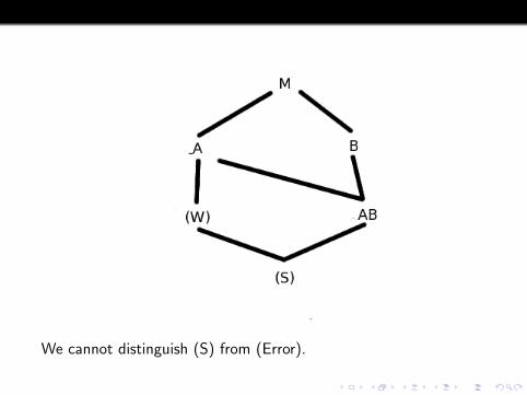
We cannot distinguish (S) from (Error).

Note that this Hasse diagram looks just like the one we saw forcheese raters.

Different designs can lead to the same model structure.

We can just use lmer() or lme() with a random effect for the wholeplots and proceed as usual.

Comparisons at whole plot level are less precise than those at splitplot level. Similarly, less power at whole plot levee.

Generalizations

More than two factors. We can have multiple factors at whole plotlevel and/or split plot level.

The design at the whole plot level could be any one of ourblocking designs. RCB is very common at WP level.

Can do additional balancing at split plot level. E.g., take a crossover design (replicated LS), then add a second factor at the wholeplot (subject) level.

Two whole plot factors, one split plot factor.

One whole plot factor, two split plot factors.

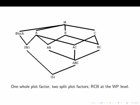
One whole plot factor, two split plot factors; RCB at the WP level.

Crossover design in B (Latin sq), but A randomly applied tosubjects.

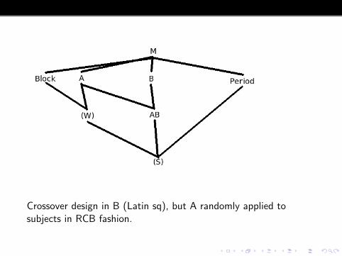
Crossover design in B (Latin sq), but A randomly applied tosubjects in RCB fashion.

Some books only talk about split plots with whole plot blocking.

Some of these books use a model of random blocks that interactwith the whole plot factor and the split plot factor. This is not thesame as what I have described.

These books tend to have an engineering orientation, so I call thisthe industrial split plot model.

I don’t use this model.

Split split plot designs

Once you have the idea of splitting units into smaller units, youcan split more than once.

A split split plot has three sizes of units: whole plots that are madeup of split plots which are made up of split split plots.

Two levels of nesting in the unit structure: split split plots nestinto split plots, and split plots nest into whole plots.

You need at least three factors: a whole plot treatment factor, asplit plot treatment factor, and a split split plot treatment factor.

A : 5⇓

B : 2⇒

{ 5:2:2 ← C : 25:2:3 ← C : 35:2:1 ← C : 1

B : 1⇒

{ 5:1:1 ← C : 15:1:2 ← C : 25:1:3 ← C : 3

B : 3⇒

{ 5:3:3 ← C : 35:3:2 ← C : 25:3:1 ← C : 1

7 by 3 by 3 split split plot. This whole plot received level 5 offactor A; the three split plots and nine split split plots are assignedas shown.

With three levels of randomization and three sizes of units, we getthree random terms: one for whole plots, one for split plots, andone for split split plots (indistinguishable from error).

We can have various kinds of blocking at the whole plot level.

We can have more than one factor at each randomization level.

Follow the randomization! Counting factors is not a way todistinguish between split plot designs and split split plot designs(or even CRD).

Split split plot with CRD at WP level.

Split blocks/strip plots etc.

Once you get the idea of splitting (nesting) units, you could go allthe way to a split split split split split plot if you wanted. I don’tthink I’ve seen beyond split split plot in the wild.

However, we now have unit structure. We have seen nesting units.

Can units cross? Yes, they can.

We can build designs with unit structures that have nesting,crossing, or both. Then we layer the treatment structure on top ofthat!

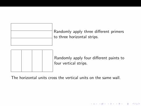
Randomly apply three different primersto three horizontal strips.

Randomly apply four different paints tofour vertical strips.

The horizontal units cross the vertical units on the same wall.

Randomly apply three different varietiesto horizontal strips. Randomly applytwo different fertilizers to the two hori-zontal substrips.

Randomly apply four irrigation levels tofour vertical strips.

We have a blocked split plot in the horizontal units and an RCB inthe vertical units, and the vertical units cross the horizontal units.

We typically need replication in blocks for this to work well.Above, blocks were the walls or the large chunks of land.

The basic model is to have a random effect for each kind of unit(randomization) and wherever units cross.

Split block, also called strip plot. Ignore paint, it’s an RCB onprimer; ignore primer, it’s an RCB on paint.

Split plot crossing an RCB. Ignore irrigation, it’s a split plot in Vand F. Ignore F, it’s a strip plot in I and V.

Repeated Measures

Repeated measures look like split plots, but there is norandomization at the “split plot” level.

Typically the “split plot” treatment factor is time, and withrepeated measures we just keep measuring the same unitrepeatedly over time.

Time does not like to be randomized,1 so it’s not a split plot.

Another version arises when we can measure the same thingmultiple ways. We literally just get multiple measurements.

1Insert generic Dr. Who reference.

In the repeated measures terminology:

“Whole plots” are called subjects.

“Whole plot” treatment factors are called grouping factors.

“Split plot” treatment factors are called trial factors.

In our example, we prepare emulsions using three differentemulsifiers. We then measure each separate emulsion over time.

Each emulsion is the “subject.” The emulsifiers form the groupingfactor. Time is the trial factor.

Kind of looks like a split plot, but no randomization.

What is happening is that we have experimented at the subjectlevel, but we observe a vector of responses across the trial level.

This vector of responses is probably correlated, not independent.

Some kind of correlation is potentially present among units we usein experimentation, but randomization of treatments to unitsscrambles the correlation to the point it can usually be ignored.

But, no randomization, no scrambling; the correlation comesthrough unaltered and potentially affecting results.

Analysis

Potential approaches:

1 Full multivariate analysis.

2 Univariate summaries.

3 Univariate analysis.

4 Modified univariate analysis.

5 Model the correlation.

1. Full multivariate analysis. This requires a lot of data to workwell and many techniques we have not discussed. Take Stat 5401if you are interested in this approach.

2. Univariate summaries. Here you create some kind of statisticfrom the trial data for each subject, for example, the rate ofchange over time. You then treat this as the response for a subjectand do standard analysis. By looking at different summaries youcan examine different aspects of trial factor effects.

Univariate summaries are a legitimate approach, but you need tochoose the right summary (or summaries), and you have to figureout the relationship if you have more than one summary.

3. Univariate analysis approach. This approach says assume thereis a random subject effect and that this effect interacts with everytrial factor. With just a single trial factor this is equivalent to thestandard split plot analysis.

If nature has been very kind to you and the data at the trial levelhave a covariance that satisfies a special condition, then theunivariate approach is legitimate.

If the trial factor has only two levels, then the univariate approachis always legitimate.

If you were unlucky and didn’t get the special form of covariance,then tests at the trial factor level tend to be liberal.

The special condition (the Huynh-Feldt condition) is that alldifferences of repeated measures have the same variance.

One case that satisfies the HF condition is sphericity: all variancesare the same and all correlations between trial levels within asubject are the same (the correlations don’t have to be zero).

For multiple trial factors there is a generalization of sphericitycalled compound symmetry.

There is a Mauchly Test for the HF condition, but it is verydependent on normality.

4. Modified univariate analysis. The modifications are for the“treat it like a split plot” approach with old school mixed effectsanalysis. The modifications adjust the tests in an attempt to makethem less liberal (but not conservative).

There is a Greenhouse-Geisser adjustment and a Huynh-Feldtadjustment. Both of these reduce the error DF for trial level testsby some factor estimated from the data.

5. Model the correlation. The approach is possible with REMLcomputations; it models and estimates the correlation, and thentakes the correlation into account.

We generally anticipate positive autocorrelation over time betweenthe observations for a single subject (separate subjects still beingindependent). There are many potential models for this, butautoregressive of order one (AR1) is the simplest and mostcommon.