spectrum management technical handbook
TRANSCRIPT

TECHNICAL NOTE SERIES
NTIA TN 89-2
SPECTRUM MANAGEMENT
TECHNICAL HANDBOOK
l
NTIA TECHNICAL NOTE 89-2
SPECTRUM MANAGEMENT TECHNICAL HANDBOOK
U.S. DEPARTMENT OF COMMERCE Robert A. Mosbacher, Secretary
Alfred C. Sikes, Assistant Secretary for Communications and Information
JULY 1989

ACKNOWLEDGEMENT
NT IA acknowledges the efforts of Mark Schellhammer in the completion of Phase I of this handbook (Sections 1 -3) . Other portions wil l be added as resources are available.
ABSTRACT
This handbook is a compilation of the procedures, definitions, relationships and conversions essential to electromagnetic compatibi l ity analysis. It is intended as a reference for NTIA engineers.
KEY WORDS
CONVERSION FACTORS COUPLING EQUATIONS
DEFIN ITIONS ·TECHNICAL RELATIONSH IPS
i i i

I
I
TABLE OF CONTENTS
Subsection Page
S ECTION 1
TECH NICAL TERMS: DEFI N ITIONS AN D NOTATION
TERMS AND DEFIN ITIONS . . . . . . . . . . . . . . . . . . . . . . . . . . . . . . . . . . . . . . . . 1-1 GLOSSARY OF STANDARD NOTATION . . . . . . . . . . . . . . . . . . . . . . . . . . . . . . . 1 -1 3
S ECTION 2
TECH NICAL RELATIONSHIPS AND CONVERSION FACTORS
INTRODUCTION . . . . . . . . . . . . . . . . . . . . . . . . . . . . . . . . . . . . . . . . . . . . . . . . 2-1 �
TRANSM ISSION LOSS FOR RADIO LIN KS . . . . . . . . . . . . . . . . . . . . . . . . . . . . . 2-1 Propagation Loss . . . . . . . . . . . . . . . . . . . . . . . . . . . . . . . . . . . . . . . . . 2-1 Transmission Loss . . . . . . . . . . . . . . . . . . . . . . . . . . . . . . . . . . . . . . . . Free-Space Basic Transm ission Loss . . . . . . . . . . . . . . . . . . . . . . . . . . . Basic Transmission Loss . . . . . . . . . . . . . . . . . . . . . . . . .. . ... . .. . . . Loss Relative to Free-Space . . . . . . . . . . . . . . . . . . . . . . . . . . . . . . . . . . System Loss . . . . . . ; . . . . . . . . . . . . . . . . . . . . . . . . . . . . . . . . . . . . . .
2-2 2-2 2-2 2-2 2-3
Total Loss . . . . . . . . . . . . . . . . . . . . . . . . . . . . . . . . . . . . . . . . . . . . . . 2-3 ANTENNA CHARACTERISTICS . . . . . . . . . . . . . . . . . . . . . . . . . . . . . . . . . . . . . . 2-3
Antenna Directivity . . . . . . . . . . . . . . . . . . . . . . . . . . . . . . . . . . . . . . . . Antenna Gain and Efficiency . . . . . . . . . . . . . . . . . . . . . . . . . . . . . . . . . . Effective Aperture Area . . . . . . . . . . . . . . . . . . . . . . . . . . . . . . . . . . . . . Far Field Region for Aperture Antennas . . . . . . . . . . . . . . . . . . . . . . . . . . Near Field Region for Aperture Antennas . . . . . . . . . . . . . . . . .. . . . . . . .
POWER AND ELECTRIC FI ELD INTENSITY . . . . .. . . . . . . . . . . . . . . . . . . . . . . . Received Power Spatial Density to Received Power . . . . . . . . . . . . . . . . . Received Electric Field Intensity to Received Power . . . . . . . . . . . . . . . . . Recieved Voltage to Received Electric Field Intensity . . . . . . . . . . . . . . . . Received Voltage to Received Power . . . . . . . . . . . . . . . . .. . . . . . . . . . Transmitted Power to Field Intensity . . . . . . . . . . . . . . . . . . . . . . . . . . . . Field Intensity at Different Distances in the Far-field Region . . . . . . . . . . . .
v
2-3 2-3 2-4 2-4 2-5 2-5 2-5 2-6 2-7 2-7 2-8 2-8

TABLE OF CONTENTS (Continued)
Subsection Page
· RECEIVER NOISE LEVEL . . . . . . . . . . . . . . . . . . . . . . . . . . . . . . . . . . . . . . . . . . 2-8 System Noise Temperature . . . . . . . . . . . . . . . . . . . . . . . . . . . . . . . . . . 2-8 Antenna Noise Temperature . . . . . . . . . . . . . . . . . . . . . . . . . . . . . . . . . . 2-9 Receiver Noise Temperature . . . . . . . . . . . . . . . . . . . . . . . . . . . . . . . . . 2-1 1 Receiver Noise Figure . . . . . . . . . . . . . . . . . . . . . . . . . . . . . . . . . . . . . . 2-1 2 Noise Summary . . . . . . . . . . . . . . . . . . . . . . . . . . . . . . . . . . . . . . . . . . 2-13
RECEIVER SENSITIVITY . . . . . . . . . . . . . . . . . . . . . . . . . . . . . . . . . . . . . . . . . . . 2-1 4 DECIBEL CONVERSIONS . . . . . . . . . . . . . . . . . . . . . . . . . . . . . . . . . . . . . . . . . 2-1 5
Conversions to d B . . . . . . . . . . . . . . . . . . . . . . . . . . . . . . . . . . . . . . . . 2-1 5 Decibel Conversions for Power . . . . . . . . . . . . . . . . . . . . . . . . . . . . . . . . 2-1 5 Decibel Conversions for Voltage (also Field Intensity) . . . . . . . . . . . . . . . . 2-1 5
M ISCELLANEOUS CONVERSIONS . . . . . . . . . . . . . . . . . . . . . . . . . . . . . . . . . . . 2-1 5 Maximum Radio Line of Sight Distance Over a Smooth Earth . . . . . . . . . . 2-1 5 Decibel Conversions for Frequencies . . . . . . . . . . . . . . . . . . . . . . . . . . . 2-1 5 Power Density . . . . . . . . . . . . . . . . . . . . . . . . . . . . . . . . . . . . . . . . . . . 2-1 5 Free-Space Propagation Velocity . . . . . . . . . . . . . . . . . . . . . . . . . . . . . . 2-1 6 Wavelength Conversions . . . . . . . . . . . . . . . . . . . . . . . . . . . . . . . . . . . . 2-1 6 Distance Conversions . . . . . . . . . . . . . . . . . . . . . . . . . . . . . . . . . . . . . . 2-1 6
SECTION 3
COUPLING EQUATIONS
INTRODUCTION RECEIVED POWER . . . . . . . . . . . . . . . . . . . . . . . . . . . . . . . . . . . . . . . . . . . . . . INTERFERENCE-TO-NOISE RATIO . .. . .. . .. .... . . . . ... . .. .. .. . . . . ... . CARRIER-TO-INTERFERENCE RATIO (Terrestrial Systems) . .. . . .. ... . . .. .. . . CARRIER-TO-INTERFERENCE RATIO (Satel l ite Systems) . . .. ... . .. . . . . . ... . CARRI ER-TO-NOISE RATIO . . ... ... .. . .. .... . ....... . . .. . . . . . . . .. . . MAXIMUM PERMISS IBLE I NTERFERENCE LEVEL . . . .. . . . .. .. . . . .. . . .. . . . FREQUENCY-DISTANCE SEPARATION ...... . . . . . . . . . ... . ....... .. . .. . FREQU ENCY DEPENDENT REJECTION ..... . . . .. . . . . . ... ... .. . . .. . . . .
On-Tune Rejection . . . . ..... . .. . ......... .. .. .. .. .. . ... . . . . Off-Frequency Rejection . .. ........ . .... . . . . . .. .... ..... ... . . Frequency Dependent Rejection for Pulse Interference . .. .. .. ... . ... .
vi
3-1 3-1 3-2 3-2 3-3 3-4 3-5 3-5 3-6 3-7 3-7 3-7
r
I I
. r
I
I [
I t
l

I l
I
I
l
l
l {
(
Table
3-1
Figure
2-1 2-2
TAB LE OF CONTENTS (Continued)
L IST OF TABLES
FREQU ENCY DEPEN DENT REJECTION
LIST OF FIGURES
Transmission loss for radio links Noise Comparison
vii
Page
3-8
Page
2-1 2-1 1

SECTION 1
TECHNICAL TERMS: DEFINITIONS AND NOTATION
TERMS AND DEFINITIONS
The following l ist includes technical terms and definitions often used in technical analyses for spectrum management. The l ist is intended to supplement those terms defined in the ITU Radio Regulations and the NTIA Manual of Regulations and Procedures for Federal Radio Frequency Management. Refer to these documents for additional technical terms and definitions used in spectrum management.
Adjacent Channel Interference (ACI): interference caused by a signal operating on a frequency close to the desired channel but outside its bandwidth.
Adjacent Channel Rejection: a measure of the ability of a receiver to discriminate against an undesired signal at the frequency of the adjacent channel . Adjacent channel rejection is usually expressed in dB.
Antenna Efficiency (TJ): the ratio of input power to total effective radiated power of an antenna, used as a measure of how efficiently the aperture area of an antenna is uti l ized.
Antenna Noise Temperature (Ta): the noise temperature due to externally generated noise sources appearing at an antenna input. This includes atmospheric, cosmic, man-made, sun and terrestrial noise. Antenna noise temperature is usually expressed in degrees Kelvin.
Articulation Index (AI): a measure of speech intel l igibi l ity determined by a device connected to a receiver's audio output stage. The articulation index value is a frequency-weighted signal-to-noise ratio of individual frequency sub-bands of the speech signal .
Articulation Score (AS): a measure of units of phonetical ly balanced speech, spoken by a talker, correctly repeated or checked by a listener. This is a performance index of a communications system including transmitter, medium and receiver with all parameters of the system specified.
Atmospheric Noise: noise primarily due to thunderstorms and l ightning (usual ly occurring at frequencies below 20 M Hz) .
1 -1

Bandwidth: the range of frequencies within which the performance of a system, with respect to some characteristic, falls within specified l imits. Bandwidth is expressed in Hz, kHz, MHz.
Baseband: the band of frequencies used to convey information on a transmitted signal. Baseband frequencies usually range over lower frequencies than those of the radio signal.
Basic Transmission Loss (Lb): the loss that would occur if the antennas were replaced by isotropic antennas of l ike polarization. Note that the effect of the local ground close to the antenna is included in computing the antenna gain, but not in the basic transmission loss. Basic transmission loss is usually expressed in dB.
Beam Angle: the angle between the d irection of the maximum of a major lobe or a directional null and a reference direction. Beam angle is usually expressed in degrees or radians.
Beamwidth: see Half-power Beamwidth.
Bit Energy-to-Noise Ratio (Eb/N0): the ratio of the average bit energy to noise power spectral density. It is a function of the type of coding, modulation, accessing technique and the characteristics of the amplifiers and filters used in a digital communications system. The quantity is usually expressed in dB.
C-Message Weighting: a shaped noise signal that simulates the noise characteristics of a telephone circuit.
Capture Effect: the process of an FM receiver selecting the strongest of multiple signals of the same frequency as its output. '
Carrier: the basic radio wave of specified frequency used to convey information by varying one or more of its characteristics (i .e . , amplitude, frequency and phase).
Carrier Power: the average power supplied to the antenna transmission l ine by a transmitter during one radio frequency cycle taken under the condition of no modulation. Carrier power is usually expressed in watts, mi l l iwatts, dBW, or dBm.
Carrier-to-Interference Ratio (C/1): the ratio , at the receiver RF input, of the desired carrier power to the interfering signal power which satisfies a specified receiver degradation criteria. The C /I ratio is usually expressed in dB.
Carrier-to-Noise Ratio (C/N): the ratio of the desired carrier power to the total receiver system noise power referred to the RF input. The C/N ratio is usually expressed in dB.
1 -2
[
r
[
[
r
[
L
[ l l r

!-
I
l
f
Carrier-to-Noise plus Interference Ratio (C/N + 1): the ratio of the desired carrier power to noise plus interference power contained within the receiver IF bandwidth. The ratio is usually expressed in dB.
Chip Rate: the rate of encoding in a spread spectrum system.
Cochannel Interference (CCI): the presence of an external interfering signal at the tuned frequency of a receiver. CCI can be caused by insufficient spatial or spectral signal isolation or polarization isolation and other effects.
Conducted Interference: interference resulting from conducted radio noise or unwanted signals entering a receiver by direct coupling.
Conducted Spurious Emission: the emission caused by the combining of an undesired signal with the desired signal by coupl ing into a system by conduction.
Cosmic Noise: the noise due to radio sources from outer space excluding galactic noise. Cosmic noise is negligible above 1 GHz.
Coupling Mechanism: the mechan ism by which interference is generated in the receiver (e.g . , cochannel , adjacent channel , spurious response, and intermodulation)
Cross-modulation Interference: the modulation of the carrier of one signal by an undesired signal by passing them through a nonl inear element.
dBa: the abbreviation for dBrn- adjusted, referring to noise measurements made at the receiving end of a l ine by a noise meter with F1 A-line weighting. The meter is calibrated on a 1 ,000 Hz tone so that 0 dBm will g ive a reading of +85 dBa corresponding to a reference noise power of -85 dBm.
dBaO: the abbreviation for the measure of noise power with reference to zero dBm at the zero transmission level point. Noise powers measured at any transmission level point can be expressed in dBaO by correcting the measured noise power for the difference in level between the point of measurement and the reference transmission level point.
dBi: the abbreviation for the gain of an antenna relative to an isotropic antenna.
dBmO: the abbreviation for absolute power level i n dBm, referred to, or measured at, a point of zero transmission level. The dBmO figure for a given signal characterizes it wherev�r the signal may appear elsewhere in the circuit.
1 -3
dBmOp: the abbreviation for the absolute noise power in dBm, referred to or measured at a point of zero relative transmission level , psophometrically weighted.
dBr: the abbreviation for the decibel relative level , and is used to define transmission levels at points in a circuit, with respect to the zero transmission level reference point. The signal level at any given point in the circuit when expressed in dBr is a measure of the net effect of all the losses and gains in the circuit, from the origin to the point specified.
dBrn: the abbreviation for decibels above reference noise.
dBrnc: the abbreviation for decibels above reference noise which includes C-message weighting.
Decibel (dB): a unit expression for representing the logarithm base 1 0 ratio of two values of a parameter used to characterize a system.
Deemphasis: a process of recovering the amplitude distribution of the frequency components of a signal that have been modified intentionally by the transmitter.
Degradation: a measure of the deterioration of specific characteristics of a desired signal caused by interference or noise.
Degradation Criteria: the minimum acceptable receiver system performance in the presence of interference. The receiver output degradation criteria may be expressed in terms of signal-to-interference plus noise, bit-error rate (BER) , probability of false alarm, receiver break lock, etc.
Demodulation: the extraction of a signal having the characteristics of the original baseband modulation on a transmitted carrier.
Deviation Ratio: the ratio of the maximum frequency deviation to the maximum modulation frequency of a frequency or phase modulated signal. The deviation ratio is usually expressed in dB.
Diplexer: a circuit that switches an antenna to either the transmitter or receiver and also protects the receiver from damage during transmission.
Directivity: a ratio measure of the ability of an antenna to concentrate radiated power in a given direction (usual ly that of maximum radiation intensity) to the radiation intensity averaged over all directions.
1 -4
r
I
I
I
[
r
I
I l l
l
l
I
I \ l

Distortion: any deviation of an input-output signal relationship over a range of frequencies, phases or ampl itudes.
Diversity, Frequency: a method of transmission and reception intended to compensate the effect of fading whereby the same information is transmitted and received simultaneously on two or more carrier frequencies.
Diversity, Polarization: a method of transmission and reception intended to compensate the effects of fading by using differently polarized antennas to handle the same information.
Diversity, Space: a method of transmission and reception intended to compensate the effects of fading whereby the same information is simultaneously transmitted or received using more than one antenna with a spatial separation at one or more of the communication links.
Doppler Effect: the effective change of frequency caused by the relative motion between a source and receptor.
Duty Cycle: the ratio of the transmitter on-time to off-time during one radio frequency cycle.
Dynamic Range: The amplitude range of an input signal that will produce an undistorted signal at the output of a source. Dynamic range is usually expressed in dB.
Earth Noise: the noise due to radiation of the earth. Sometimes also referred to as terrestrial noise. The average noise temperature of earth noise is 290° K, as seen from an antenna on the ground.
Effective Antenna Height: the height of an antenna equal to the height structure of an antenna plus the average terrain elevation along the transmission path.
Effective Area: the ratio of the available power at the terminals of a receiving antenna in a given direction (usually, the direction of maximum radiation intensity is implied) to the power flux density of a plane wave incident on the antenna from that direction, with the wave polarized to match the antenna.
Electric Field Strength: the magnitude of the potential gradient in an electric field expressed in units of potential difference per unit length in the direction of the gradient. Field strength is usual ly expressed in volts/meter, microvolts/meter, dBV jm or dBtLV jm.
1 -5
Electromagnetic Interference: any undesired electromagnetic emission received by a system, which causes degradation of specified performance measures.
Emission Bandwidth: the range or spectrum of frequencies of any desired or undesired electromagnetic energy propagated from a source by radiation.
FM Improvement Threshold: the input carrier-to-noise ratio, C/N, above which the peaks of the signal begin to exceed the peaks of the noise and FM quieting begins in an FM receiver. This effect occurs when the power of the input signal is approximately 5- 1 0 dB above the power of the noise.
FM Quieting: the reduction of noise output of an FM receiver in the presence of a signal. Sensitivity is sometimes defined in terms of a specified level of quieting.
Fade Margin: the amount by which a received signal level may be reduced without causing the system output to fall below a specified signal-to-noise threshold. Fade margin is usually expressed in dB.
Fading: the variation of the intensity and relative phase of frequency components of radio field due to the variation of propagation characteristics with time.
Far-field Region: the region where the angu lar electromagnetic field distribution is independent of distance from the source.
Free Space Basic Transmission Loss (Lb1): the transmission loss that would occur if the antennas were replaced by isotropic antennas located in a perfectly die lectric homogeneous, isotropic and unlimited environment. This loss, also referred to as the wave spreading loss, is usually expressed in dB.
Frequency Dependent Rejection (FOR): the sum of the frequency rejection provided by a receiver to an input signal as a result of both the l imited bandwidth of the receiver and the detuning of the signal frequency (i .e . , the sum of the on-tune rejection OTR, and offfrequency rejection, OFR) .
Frequency Diversity: see Diversity, Frequency.
Gain, Available (Ga): the ratio of the available power at the system output to the available power of the source output. Avai lable gain is a function of frequency and is usually expressed in dB.
1 -6
[
[
r I [
I I I l I
l
l
I
l
I

------ ...
Gain, Half-Wave Dipole: the antenna gain when the reference antenna is a half-wave dipole isolated in space whose equatorial plane contains the given direction of propagation.
Gain, Antenna (G1, Gr): the measure of the abil ity of an antenna to concentrate power in a given direction, usually within the main lobe, referenced to a standard antenna (usually an isotropic antenna) . Antenna gain is usually expressed in dBi .
Gain-to-Noise Temperature Ratio (G/T): the figure of merit, for receiving stations, which is a ratio of the antenna power gain to the total noise temperature at the receiver input referred to the antenna terminals . Gain-to-noise temperature ratio is usually expressed in dB/K.
Galactic Noise: the noise due to radio stars in the galaxy. Galactic noise is negligible at frequencies greater that 1 GHz.
Half-power Beamwidth within the antenna mainlobe, the ang le between the two directions in which the radiated power density is one-half the maximum value.
Harmonic Distortion: nonlinear signal distortion of a system characterized by output harmonics other than the fundamental component when the input wave is a sinusoid.
High-Power Effects: the undesired detection of radiated signals via means other than the antenna.
Image Frequency: a spurious frequency response, in a superheterodyne receivers, separated from the tuned frequency
. by twice the intermediate frequency.
Image Rejection Ratio: relates the specified level of a signal at the image frequency to the level of a signal at the tuned frequency producing the same output power.
Insertion Loss: the ratio of input signal power to the output signal power due to the insertion of a device at some point in a transmission line between an antenna and the receiver or transmitter, in dB. Radome losses, which occur beyond the antenna, are frequently added as part of the system insertion loss when performing coupling calculations.
Interference Coupling Ratio: the ratio of the power of a desired signal in a circuit to the power of an undesired signal. The interference coupling ratio is usually expressed in dB.
Interference Guard Bands: the two bands of frequencies additional to, and on either side of, the required signal bandwidth , which minimize the possibil ity of interference.
1 -7
Interference Margin: the measure of the amount by which the power of the interfering signal must increase to exceed the level required to cause harmful interference. The interference margin is usually expressed in dB.
Interference plus Noise-to-Noise Ratio (I+ N/N}: the ratio of the interfering signal plus noise power to the noise power. It is usually taken at the receiver output and expressed in dB.
Interference-to-Noise Ratio (1/N}: the ratio at the receiver RF input of interfering signal power to the total receiver system noise power referred to the RF input, usually expressed in dB. A 1/N which satisfies a specified receiver degradation criteria is often determined as a means to evaluate a receiver for acceptable performance in a noise-limited situation.
Intermediate Frequency Interference Ratio: the ratio of the field strength at a specified frequency in the IF band to the field strength at the desired frequency. The intermediatefrequency interference ratio is usually expressed in dB.
lntermodulation Distortion: the result of a nonlinear process in a system where two or more input signals' spectral components produce new components equal to the sums and differences of integral multiples of the component frequencies. Note that harmonic components are not included as part of intermodulation distortion.
lntermodulation Interference: the interference on the desired signal produced by the mixing of two or more signals in a nonlinear stage or other nonlinear device.
lntermodulation Spurious Emission: the external radio frequency emission of a transmitter resulting from the nonlinear mixing process in the final stage where external RF power is coupled through the antenna output.
Isotropic Antenna: an idealized model for a lossless antenna radiating energy equally in all directions from a point source.
Jansky: a unit of spectral power flux density defined as 1 o-26 W fm2 /Hz.
Man-made Noise: the noise due to man-made sources such as electrical machinery and automobile ignition. This noise ranges in frequencies up to 1 GHz.
Mid-pulse Minimum Visible Signal (MPMVS}: the minimum input pulse signal power level that permits visibil ity of the center of the output pulse. This level is obtained by initially setting the input signal above the detection threshold and then slowly decreasing the amplitude.
1 -8
r
I
r r [
r
I
l I l
I I [

r
(
Multipath: the condition existing when more than one ray path is available for radio energy to travel from a transmitter to the receiver.
Narrow-band Interference: an electromagnetic disturbance of power spectral density lying · completely within the passband of a receiver.
Near-field Region: the region in which the relative angular distribution of the field is dependent on the distance from the antenna. This is the region in which the relative phase and ampl itude relationships of field contributions from different e lements of the antenna change significantly with distance.
Noise Factor (F): the ratio of the actual I F output noise power (including image frequency contributions) to that which would remain if the system were at a standard noise temperature, 290 K.
Noise Figure (NF): the decibel expression of the noise factor.
Noise Power Ratio (NPR): the ratio of noise in a baseband telephony system measured in a clear channel when al l other channels are loaded with noise. The NPR wil l vary with loading so that the results are expressed as a series of curves.
Noise Temperature: the temperature, expressed in Kelvins, of a passive system having an available noise power per unit bandwidth equal to the actual terminals. The standard reference temperature for noise measurements is 290 K.
Off-frequency Rejection (OF:'R): the ratio of the undesired signal power at the receiver I F output, as a function of frequency detuning, to the undesired signal power received when the transmitter and receiver are tuned to the same frequency.
Omnidirectional Antenna: an antenna having an essentially nondirectional pattern in a given plane of the antenna and a directional pattern in any orthogonal plane.
On-tune Rejection (OTR): the rejection of an undesired co-tuned signal , as a resu lt of an emission spectrum exceeding the receiver bandwidth.
Out-of-band Interference: the interference from undesired signals at frequencies n9t within the desired signal passband.
Peak Power (P): the maximum instantaneous power attained by a waveform over the duration of measurement.
1 -9

Performance Criteria: measures of the minimum acceptable receiver system performance in the presence of receiver noise only. The receiver output performance criteria may be expressed in terms of signal-to-noise ratio, bit-error rate (BER) , tangential sensitivity, etc.
Polarization: the orientation of any field (e lectric, magnetic) of an electromagnetic wave. Types include l inear, circular and el l iptical.
Polarization Diversity: see Diversity, Polarization.
Power (P): the amount of energy which flows out of (or into) a region or circuit per unit time. Whenever the power of a radio transmitter is referred to, it is expressed as peak envelope power, mean power, or carrier power. For different classes of emission, the relationships between these forms, under the conditions of normal operation and without modulation, are contained in CCIR recommendations, which may be used as a guide. Power is usually expressed in watts, mi l liwatts, d BW or dBm.
Power Density, Spatial (P d) : the d istribution of power per unit area over a propagating medium. Power density is usually expressed in mill iwattsjm2 and dBm/m2•
Power Flux Density (PFD): the emitted power per unit cross-sectional area normal to the direction of propagation per unit frequency. Power flux density is usually expressed in wattsjm2/Hz and dBW jm2 /Hz.
Power, Transmitter (Pt) : the total power emitted from a transmitter. Output power is usually expressed in watts, mi l l iwatts, dBW or dBm.
Power, Receiver (Pr): the product of the power density at a specified distance from the transmitter antenna in the desired direction, P d' and the effective aperture area of the receiving antenna, Ar. Receiver power is usually expressed in watts, dBW or dBm.
Power Spectral Density (PSD): the distribution of power per unit bandwidth . Power spectral density is usually expressed in watts/Hz, dBW /Hz and dBm/Hz.
Pulse Width: the time interval between half voltage points in the t ime waveform of a pulse signal.
Preemphasis: a method of modifying the amplitude distribution with frequency to compensate for nonuniform frequency response of transmitter circuits.
1 -1 0
I
[
I
I
I
[
I
I
I
I l
[
l
l
I

Processing Gain (PG): the ratio of the baseband output signal-to-noise ratio to the receiver input signal-to-noise ratio due to receiver processing. The processing gain is usually expressed in dB.
Propagation Loss (LP): the attenuation of a radio wave which occurs when propagating between a transmitting antenna and the receiving antenna. It does not include antenna gains and is usual ly expressed in dB.
pWOp: the abbreviation for the absolute noise power in picowatts measured at a point of zero relative transmission level by a psophometer with CCITI 1 951 weighting.
Pulse Rise/Fall Time: the time interval between the 1 0% and 90% voltage points of a pulsed signal.
Radiation Efficiency: the ratio of the total power radiated by an antenna to the net power accepted by the antenna from the connected transmitter.
Radio Frequency (RF): the frequency at which electromagnetic radiation may be transmitted , received and detected as an electrical current at the wave frequency. The radio frequency is usually expressed in kHz, M Hz or GHz. "
Radome Loss: the attenuation of a signal as it passes through the antenna covering . Radome loss is usually expressed in dB.
Receiver Noise Power: the total receiver system noise power referred to the receiver RF input. Receiver noise power is usually expressed in dBm.
Receiver Noise Temperature (Tr): the effective noise temperature of a receiver due to all internally generated noise sources (ie . , amplifiers, filters, mixers, and transmission lines) . Receiver noise temperature is usually expressed in Kelvins.
Reference Frequency: the frequency which serves as a basis for comparison with other signals.
Reflection Region: the portion of a propagation path lying in the l ine of sight region and in which both the direct and reflected waves are significant components.
Reflector Antenna: an antenna consisting of one or more reflecting surfaces to shape the RF energy.
1 -1 1

Saturation, Receiver: the condition where further increases in receiver input signal level no longer results in an appreciable change in output signal level .
Selectivity: the measure of the abil ity of a receiver to discriminate between a desired signal to which it is tuned and an undesired signal having frequency components lying outside the receiver bandwidth.
Sensitivity: the level of a signal applied to a receiver input, without the antenna and transmission line, which will produce a specified output performance criteria. Sensitivity is usually expressed in dB.
Signal-to-Noise Ratio (S/N): the ratio of the desired signal power, including carrier power, to the noise power contained within the receiver IF bandwidth. The S/N ratio is usually expressed in dB.
Signal-to-Interference Plus Noise Ratio (S/1 + N): the ratio of the desired signal power, including carrier, to the power of the interference and noise referred to the IF output. This ratio is usually expressed in dB.
SINAD: the acronym for signal plus noise plus distortion to noise plus distortion ratio at the receiver output, usually expressed in dB. The signal plus noise plus distortion is the signal power recovered from a modulated RF carrier, and the noise plus distortion is the residual signal power present after the signal is removed. This ratio is a measure of receiver output quality.
Solid-beam Efficiency: the ratio of the power received over a specified solid angle when an antenna is i l luminated isotropically by uncorrelated and unpolarized waves to the total power received by the antenna.
Spurious Response: a response in the receiver IF bandpass produced by the fundamental or harmonic of an undesired signal mixing with the fundamental or harmonic of the receiver local oscil lator.
Squelch: A circuit that sets a threshold that signals must exceed to produce an audio output of a receiver.
Standard Noise Temperature (T J: the sum total of antenna noise temperature, T a' and the receiver noise temperature of a receiver, Tr. System noise temperature is expressed in Kelvins.
1 -1 2
[
r.
I
I
r
[ I r I
l
l [
I
I

Threshold Signal-to-Interference Ratio (T /1): the m1mmum signal-to-interference power required to provide a specified degradation criteria. T /I is usually expressed in dB.
Total Loss (�): also referred to as net path loss, is the ratio , usually expressed in dB, between the power supplied by the transmitter of a radio link _and the power supplied to the corresponding receiver under real installation, propagation and operational conditions.
Transmission Loss (L): the ratio , for a radio l ink, between the power radiated by the transmitting antenna and the power that would be available at the receiving antenna terminals, P/. L is usually expressed in dB.
System Loss (LJ: the ratio, for a radio link, between the radio frequency power input to the terminals of the transmitting antenna and the resultant radio frequency signal power avai lable at the terminals of the receiving antenna. L5 is usually expressed in dB.
GLOSSARY OF STANDARD NOTATION
ACI Ae AI AS B BIF c C/1 C/N C/(N + I) d D dB
77 Eb/No EMC e. i . r.p . e. r.p. F FOR Gl Gr
Adjacent Channel Interference Antenna Effective Aperture Articulation Index Articulation Score Bandwidth I F Bandwidth Carrier Power Carrier-to-Interference Ratio Carrier-to-Noise Ratio Carrier-to-Noise plus Interference Ratio Antenna Directivity Distance Decibel Antenna Efficiency Bit Energy-to-Noise Ratio Electromagnetic Compatibil ity Equivalent lsotropically Radiated Power Effective Radiated Power Noise Factor Frequency Dependent Rejection Gain, Isotropic Gain, Receiver Antenna
1 -1 3
[ Gt Gain, Transmitter Antenna G/T Gain-to-Noise Temperature Ratio IF Intermediate Frequency 1/N Interference-to-Noise Ratio
[ k Boltzmann Constant L Transmission Loss Lb Basic Transmission Loss · r Lbt Free Space Basic Transmission Loss LP Propagation Loss
I Lpol Polarization Mismatch Loss
Lrx Receiver Line Losses Ls System Loss
[ � Total Loss � Transmitter Line Losses NF Noise Figure [ NPR Noise Power Ratio OFR Off-frequency Rejection OTR On-tune Rejection l p Power
p Peak Power
I pd Power Density PFD Power Flux Density
pn Noise Power
I pr Power, Receiver
pt Power, Transmitter PSD Power Spectral Density [ P.G. Processing Gain RF Radio Frequency S/1 Signal-to-Interference Ratio S/N Signal-to-Interference Ratio (S + N)/N S ignal plus Noise-to-Noise Ratio I
STC Sensitivity Time Control I T Temperature Ta Antenna Noise Temperature l Tr Receiver Noise Temperature Ts System Noise Temperature
I To Standard Temperature (290° K) T/ 1 Threshold Signal-to-Interference Ratio VL Load Voltage
I vrms Root Mean Square Voltage
1 -1 4 [

SECTION 2
TECHNICAL RELATIONSHIPS AND CONVERSION FACTORS
INTRODUCTION
This section contains technical conversion factors and relationships frequently used in the analysis and ve·rification of compliance with standards of radio communication systems.
TRANSMISSION LOSS FOR RADIO LINKS
There are many ways to express the attenuation of signals transmitted between a transmitter and receiver. Transmission loss is usually defined by the fol lowing terms: system loss, total loss, propagation loss, transmission loss, basic transmission loss, free space basic transmission loss and loss relative to free space (see Figure 2-1 ) .1
pt
TX .......
p , t
TXLN LOSS
Propagation Loss
Propagation Loss (Lp
) �
Gt
G r
Transmission Loss (L)
System Loss (Ls)
Total Loss (LN
)
Figure 2-1 . Transmission loss for radio l inks.
p , r
RCLN LOSS
.......
p r
RCVR
Propagation loss, �' usually expressed in dB, is the attenuation of a radio wave propagating between a transmitting antenna and the receiving antenna. It does not include antenna gains.
1. Frazier, W.E., Handbook of Radio Wave Propagation Loss (100-10,000 MHz), National Telecommunications and Information Administration, NTIA Report 84-165, Washington, DC, December, 1984.
2-1

Transmission Loss
Transmission loss, L, is the ratio, usually expressed in dB, for a radio l ink between the power radiated by the transmitting antenna and the power that would be available at the receiving antenna terminals, P/.
Free-Space Basic Transmission Loss
Free-space basic transmission loss, Lbt' usually expressed in dB , is the transmission loss that would occur if the antennas were replaced by isotropic antennas located in a perfectly dielectric homogeneous, isotropic and unlimited environment.
Basic Transmission Loss
Basic transmission loss, Lb, usually expressed in dB, is the loss that would occur if the antennas were replaced by isotropic antennas with the same polarization as the real antennas. The effect of the local ground close to the antenna is included in computing the antenna gain, but not in the basic transmission loss.
Loss Relative to Free-Space
This is the difference between the basic transmission loss and the free-space basic transmission loss. Loss relative to free-space may be further subdivided into losses of different types, such as:
absorption loss (ionospheric, atmospheric gases and precipitation) ;
diffraction loss, as for ground waves;
effective reflection or scattering loss, as in the ionospheric case including the results of any focusing or defocusing due to the curvature of a reflecting layer;
polarization coupling loss, which may arise from any polarization mismatch between the antennas for the particular ray path considered;
aperture-to-medium coupling loss or antenna gain degradation, which may occur due to the presence of substantial scatter phenomena on the path;
effect of wave interference between the direct ray and rays reflected from the ground, other obstacles or atmospheric layers.
2-2
r [ r
r I
I L
r
l l [ [

System Loss
System loss, L5, is the ratio, usually expressed in dB, for a radio l ink, of the radio frequency power input to the terminals of the transmitting antenna, P•', and the resultant radio frequency signal power available at the terminals of the receiving antenna, P / .
Total Loss
Total loss, 1;, is the ratio, usually expressed in dB, between the power supplied by the transmitter of a radio l ink and the power supplied to the corresponding receiver under real installation, propagation and operational conditions. It includes transmitter and receiver line losses.
ANTENNA CHARACTERISTICS
Antenna Directivity
Antenna directivity is the measure of the ability of an antenna to concentrate radiated power in a region of space or, conversely, to absorb energy from an incident wave. Antenna directivity may be expressed by the ratio:
d ( 8 ,cp) = _ _ P_o_w
_e_r
_r
_ad
_i_at
_e
_d
_p_e_r
_u
_n
_it
_s
_o
_l id_
a_n
_g l
_e_
Total radiated power/47r
Antenna Gain and Efficiency
(2-1)
The antenna gain, G(8 ,cp), is different from the directivity by a factor, usually less than unity, which takes the efficiency of the antenna into account. Since dissipative losses are inherent in any antenna design, not all the input power is radiated by the antenna. Therefore, G(8 ,cp) is a more practical measure of the directional properties of antennas. The gain G(8 ,cp) may be defined by:
G (8 ,cp) - Power radiated per unit solid angle
Total input power /47r
2-3
(2-2)
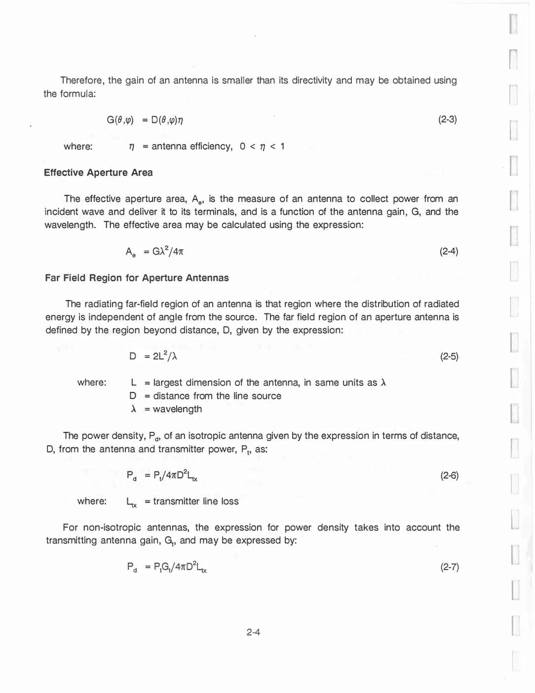
Therefore , the gain of an antenna is smaller than its directivity and may be obtained using the formula:
where:
G(B ,cp) = O(B ,cp)TJ
TJ = antenna efficiency, 0 < TJ < 1
Effective Aperture Area
(2-3)
The effective aperture area, Ae, is the measure of an antenna to collect power from an incident wave and deliver it to its terminals, and is a function of the antenna gain, G, and the wavelength. The effective area may be calculated using the expression:
(2-4)
Far Field Region for Aperture Antennas
The radiating far-field region of an antenna is that region where the distribution of radiated energy is independent of ang le from the source. The far field region of an aperture antenna is defined by the region beyond distance, 0, given by the expression:
where: L = largest dimension of the antenna, in same units as A D = distance from the line source A = wavelength
(2-5)
The power density, Pd, of an isotropic antenna given by the expression in terms of distance, 0, from the antenna and transmitter power, P., as:
(2-6)
where: � = transmitter line loss
For non-isotropic antennas, the expression for power density takes into account the transmitting antenna gain, G., and may be expressed by:
(2-7)
2-4
r [ [
r I
[ I I
l l I l
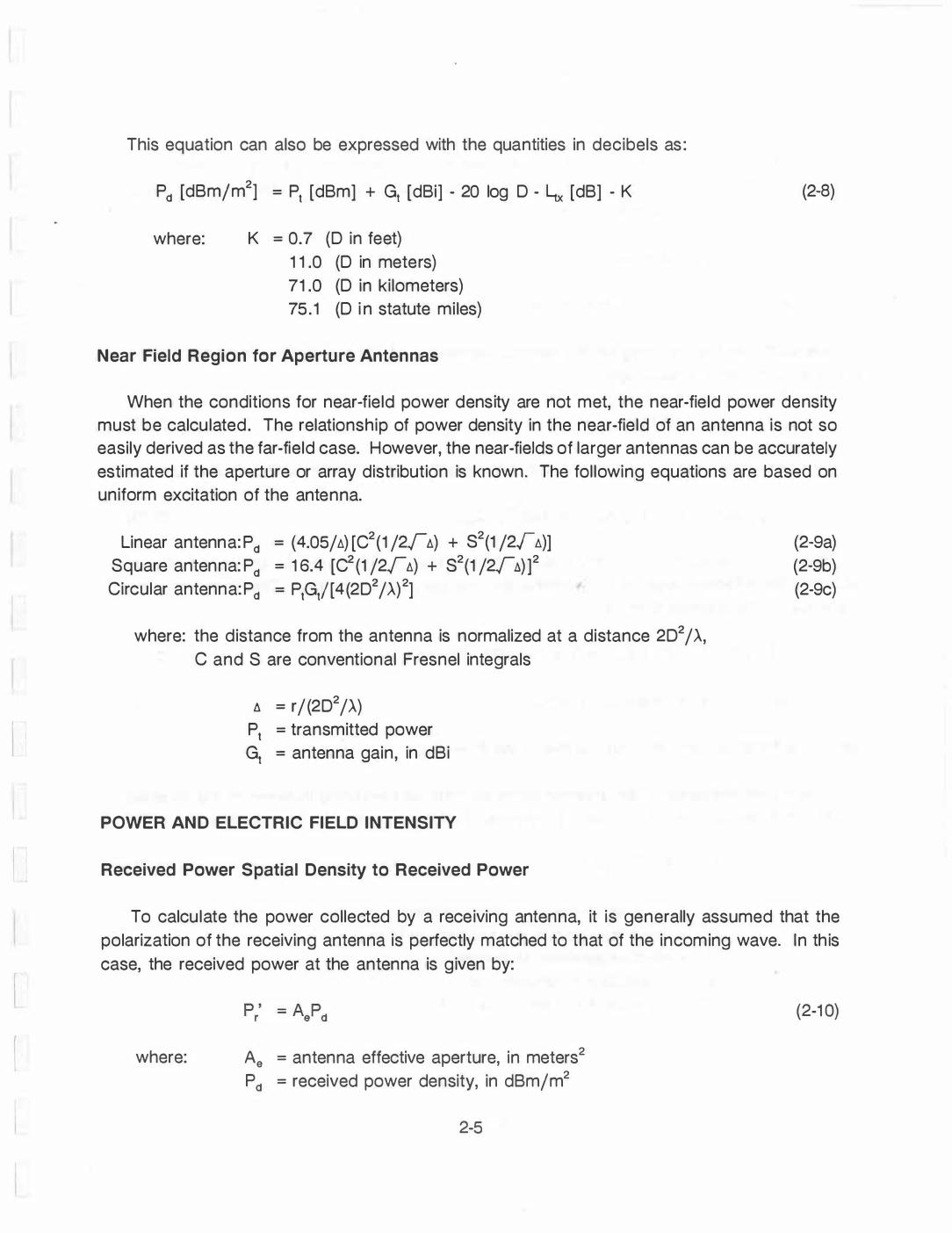
This equation can also be expressed with the quantities in decibels as :
Pd [dBmjm2] = Pt [dBm] + Gt [dBi] - 20 log 0 - l.x [dB] - K
where: K = 0.7 (0 in feet) 1 1 .0 (0 in meters) 71 .0 (0 in kilometers) 75 . 1 (0 in statute mi les)
Near Field Region for Aperture Antennas
(2-8)
When the conditions for near-field power density are not met, the near-field power density must be calculated. The relationship of power density in the near-field of an antenna is not so easily derived as the far-field case. However, the near-fields of larger antennas can be accurately estimated if the aperture or array distribution is known. The fol lowing equations are based on uniform excitation of the antenna.
Linear antenna: Pd = (4.05/ll) [C2(1 /2Fll) + S2(1 /2Fll)] Square antenna: Pd = 1 6.4 [C2 (1 /2Fll) + S2(1 /2Fl1) ]2
Circular antenna: Pd = PtG/[4(202 /.A)2]
where: the distance from the antenna is normalized at a distance 202/.A, C and S are conventional Fresnel integrals
a = r/ (202/.A) Pt = transmitted power Gt = antenna gain, in dBi
POWER AND ELECTRIC FIELD INTENSITY
Received Power Spatial Density to Received Power
(2-9a) (2-9b) (2-9c)
To calculate the power collected by a receiving antenna, it is generally assumed that the polarization of the receiving antenna is perfectly matched to that of the incoming wave. In th is case, the received power at the antenna is given by:
where: Ae = antenna effective aperture, in meters2
Pd = received power density, in dBmjm2
2-5
(2-1 0)
However, it is more correct to assume that the antenna and the wave are not matched in polarization. This mismatch wi l l reduce the power delivered to the transmission l ine. We then modify the above expression as follows:
·
where: p = polarization mismatch factor, p .2:.. 1
(2-1 1 )
We shall use the fol lowing for the decibel expression of the polarization mismatch factor, called polarization mismatch loss:
Lpol = 1 0 log p (2-1 2)
The power delivered to the antenna terminals may then be expressed in the decibel form as:
P/ [dBm] = 1 0 log Ae + 1 0 log Pd - Lpol (2- 13)
The power delivered to a antenna terminals may also be expressed by taking the relation between the effective area of an antenna and its gain into account. This power is then expressed in the decibel form as:
P/ [dBm] = Pd [dBm/m2] + Gr [dBi] - 20 log f - Lpol + 38.5
where: f = frequency in M Hz
Received Electric Field Intensity to Received Power
(2-14)
The power del ivered to the antenna terminals may be calculated in terms of the received electric field intensity incident upon the antenna. This is expressed by the equation:
where: P/ = received power at antenna terminals, in watts Erms = root mean square electric field, in V /m
Ae = effective aperture, in meters2
p = polarization mismatch factor Z = impedance of free space, 377
2-6
(2-1 5)
[
[ . r r [
I [ [
I
l
I

) l
Using the relation between the effective area of the antenna and its gain, we can express the power del ivered to the antenna terminals in terms of its gain and e lectric field intensity as:
where: c = speed of l ight, 3 X 10⁸ meters/second Z = impedance of free space, 377
(2-16)
The power delivered to the antenna terminals may be expressed in its decibel form as:
P/ [dBm] = Erms [dBV /m] + Gr [dBi] -· Lpor- 20 log F [MHz] + 42.7 6K (2-17)
or
P/ [dBm] = Erms [dBJ.LV /m] + Gr [dBi] - �01 - 20 log F [M Hz] - 77.2 0 /L
Received Voltage to Received Electric Field Intensity
The received electric field intensity may be calculated when the voltage at the receiving antenna terminals, V,n, rms' is measured. In decibel form, this is g iven by the equation:
Erms [dBJ.LV /m] = V,n,rms [dBJ.LV] + 20 log f [MHz] • Gr [dBi] + �01 - K
where: K = 29.8 (50 ohm load) 31.6 (75 ohm load) 37.6 (300 ohm load)
Received Voltage to Received Power
(2-18)
The received power at the antenna terminals, P/, may be expressed in terms of the (e.ceived voltage at the antenna terminals, V,n,rms' by the expression:
P/ [dBm] = V,n,rms [dBJ.LV] - K
where: K = 1 07.0 (50 ohm load) 1 08.8 (75 ohm load) 114.8 (300 ohm load)
2-7
(2-19)

Transmitted Power to Field Intensity
Field intensity may be expressed in terms of the transmitted power by the fol lowing:
E [dBJ.LV /m] = P1 [dBm] + G1 - � - 20 log 0 + K (2-20)
where:
for:
K = 1 1 5.0 (0 in feet) 105.0 (0 in meters) 45.0 (0 in kilometers) 41.0 (0 in statute miles)
377 ohm load (free space)
Field Intensity at Different Distances in the Far-field Region
The electric field intensity attenuates linearly with distance in free space. Therefore, it is simple to calculate the field at different distances in free-space by the relation:
where : E1 = rms e lectric field intensity at distance 01 E2 = rms electric field intensity at distance 02 01 = distance from transmitter with E1 present 02 = distance from transmitter with E2 present
(2-21 )
When the electric field is measured at some point in free-space, say 01 , then it is a simple calculation to get the field intensity, E2, at 02 by re-arranging the above:
(2-22)
By calcu lating the field intensity at this point in space, the power density is calculated by the expression:
p d = Erms2 /377
RECEIVER NOISE LEVEL
. '
(2-23)
The performance of a radiocommunication receiver depends on noise sources both internal and external to the receiver. All receiver systems exhibit a threshold that must be exceeded by
2-8
! I I r
l
( I I I I
I !
I
the desired signal at the demodulator input. This threshold effect is determined by the total noise power at the demodulator which is a function of the receiving systems I F bandwidth.
System Noise Temperature
The total noise power in the receiving system is represented by a system noise temperature, Ts, which represents the total available noise power referred to the receiver input terminals and is given by:
where: N = noise power, in watts k = Boltzmann's constant, 1 .38 X 1 o-23 joule/Kelvin
Ts = system noise temperature, in Kelvin B,F = I F bandwidth
The system noise temperature is considered to consist of two components:
(2-24)
I (2-25)
where: Ta = antenna noise temperature, which includes the contribution of noise power at the receiver input terminals received by the antenna from external sources
Tr = receiver noise tem perature, which includes contributions from sources internal to the receiver and external preamplifier and line losses from the antenna to the receiver input. This temperature is referred to the receiver input terminals.
The above equation for the total available noise power may then be written:
(2-26)
Antenna Noise Temperature
The noise received by an antenna from natural radiating sources is important in the
[ modeling and design of com munication systems and, in practice, sets a l im it to the system noise
I
l 2-9

performance. These sources of noise2 include galactic and cosmic noise, atmospheric noise, sky noise, earth (terrestrial) noise, and man-made noise3:
- Galactic noise: noise from radio stars in the galaxy. This noise falls off rapidly at higher frequencies and has negligible effect on transmissions above 1 GHz.
- Cosmic noise: refers to radio noise from outer space excluding galactic noise. This noise has negl igible effect above 1 GHz.
- Sky noise: originates mainly from oxygen and water vapor molecules which absorb radiation and then reemit it. The frequencies at which atmospheric absorption occur is approximately 20 to 1 00 GHz and have a noise temperature of less than 290 K. The noise is also a function of elevation angle.
- Atmospheric noise: noise due to thunderstorms and l ightning. This noise ranges from the lowest frequencies to 20 M Hz where its noise temperature equals 290 K.
- Earth (Terrestrial) noise: noise due to radiation from the earth. Although this noise varies due to geography, its noise temperature is taken to be 290 K. This noise is generally the dominant factor for antennas operating close to the earth. Note, that when viewed from space, the earth temperature averages at 254 K.
- Man-made noise: noise due to electrical machinery and automobi le ignition, and is consequently higher in industrial areas. Frequencies of man-made noise range from the lowest frequencies to approximately 1 GHz.
Antenna noise temperature is also a function of antenna elevation angle. Referring to Figure 2-2, we may note that below approximately 0.5 GHz, there is negl igible effect of elevation angle on antenna noise temperature. However, frequencies greater than 0.5 GHz exhibit an elevation dependence, especially between 0 - 5 degree elevation angles with a difference of as much as 270 K. The solid l ines show typical noise received by a earth antenna, excluding the effects of rain , fog , and clouds. The dashed l ine shows noise received by a satellite antenna, cause mainly by the Earth.
2. International Telecommunication Union, Worldwide Minimum External Noise Levels, 0.1 Hz to 100 GHz, CCIR Report 670, 1986.
3. Spaulding, A.D. and Disney, R.T., Man-made noise, Part 1: Estimates for business, residential, and rural areas, Office of Telecommunications Report OT 74-38, 1974.
2-1 0
r I
r r r
r
I l
I I r
I
I
I
l

r
I
l
.. ... .:l
-.. ... v Q.
E v -
0 z
Receiver Noise Temperature
Frequency. GH�
Figure 2-2. Noise Comparison
In a receiver, noise is generated by transmission lines between the antenna and receiver, and active devices in the amplification and filtering of signals. Consequently, noise generated at earl ier stages of processing can be considerably amplified before reaching the detector. When working with low-noise receivers, a useful measure of the receiver noise is given by the effective receiver noise temperature, Tr. This is defined as the temperature of a fictitious passive radiator at the input of an ideal noise-free receiver which generates the same output noise power as that of the actual transducer connected to a noise-free termination.
The receiver noise power is given by the equation:
where: k = Boltzmann's constant, 1.38 X 1 o-23 joule/Kelvin Tr = receiver noise temperature, in Kelvins
B1F = IF bandwidth, i n Hz
2-11
(2-27)
Receiver noise temperature is also expressed in terms of the noise factor:
where: F = noise factor T0 = standard temperature, 290 K
Receiver Noise Figure
(2-28)
For conventional receivers the concept of noise factor and noise figure are used to describe the performance the system. The noise factor is based upon the concept of the signal-to-noise ratio and is defined by the equation:
where: S1 = available input signal power N1 = available input noise power = kTB,F 80 = available output signal power N0 = available output noise power
The noise factor may also be expressed in the form:
where: N0 = available output noise power Tr = receiver noise temperature, in Kelvins
B,F = bandwidth of the I F output, in Hz G = average power gain
(2-29)
(2-30)
In order to produce a unity output S/N ratio when the source temperature is 290 K, a signal power si is required and is given by the equation:
81 = FkT0 [watts/Hz] (2-31 )
The noise factor F can b e considered as a measure of the noise produced i n a practical receiver compared with an ideal receiver. We then may write:
(2-32)
2-1 2
I r I I [ ! [
I
I
I
l
l l
I l

This equation then simp lifies to the fami l iar expression:
F = 1 + Tr/T0 (2-33)
The overall noise factor of n networks (with equal bandwidths) in cascade is given by:
where:
F -1 n
F = overall noise figure from input to output F n = noise figure of the n1h stage Gn = gain of the nth stage
The noise factor is usually expressed in dB and is referred to as the noise figure:
NF [dB] = 1 0 log F
Noise Summary
Another form of the total available noise power is in terms of the noise factor, F:
(2-34)
(2-35)
(2-36)
Then for an earth-bound receiver where the pattern of the antenna sees mostly earth noise , the antenna temperature, Ta, is usually T0, 290 K. In this case, the equation for the total noise power at the antenna input becomes:
(2-37)
When we express the above in terms of the values used for the variables and an I F bandwidth of 1 MHz we obtain:
N = 1 .38 X 1 0-23 X 290 X 1 06 X F [Hz]
= 400 X 1 o-14F [mW /MHz]
2-1 3
(2-38a)
(2-38b)

This may also be expressed in its decibel form for a bandwidth in either MHz or Hz as:
N = �1 14 [dBm] + 1 0 log B1F [MHz] + NF (2-39a)
N = � 174 [dBm] + 1 0 log B1F [Hz] + NF (2�39b)
A receiver typical ly has several stages of amplifiers and filters between the input and output terminations. We therefore must take into consideration the effective noise temperature and noise figure of each stage in determining the overall performance of the system.
The receiver noise temperature of n networks in cascade is given by:
where:
T r = T n + _T_r2_+ • • • + __ T_r
_n --
Trn = effective noise temperature of the nth stage Gn = average gain of the nth stage
(2�40)
The effective noise temperature of a receiver must include the effect of losses in transmission l ines and other RF components between the antenna terminals and the receiver input. These losses are especially sign ificant when they occur in the front end of a low noise receiver. For a transmission l ine with loss, L, and operating at a temperature, TP the receiver noise temperature, T/ , is given by the equation:
(2�41 )
RECEIVER SENSITIVITY
Receiver sensitivity is defined to be the level of a signal applied to a receiver input, which will produce a specified output signal-to-noise ratio. The receiver sensitivity may be expressed by the equation:
Ss = �1 1 4 [dBm] + 1 0 log B1F [MHz] + F + S/N1n [dB] (2�42)
where: S/N1n = the receiver input S/N, which produces the specified output S/N
2-1 4
I
r I [ I [
I
I
I
I l
DECIBEL CONVERSIONS
The quantities used in frequency analysis are usually expressed in their decibel form. The fol lowing conversions can be used when it is necessary to express quantities in this form.
Conversions to dB
[dB] = 1 0 log10 P2/P1 [dB] = 20 log1 0 V2/V1
when the ratio of two powers are desired when the ratio of two voltages are desired
Decibel Conversions for Power
P [dBW] = 1 0 log1 0 P [watts] P [dBm] = 1 0 log10 P [watts] + 30
Decibel Conversions for Voltage (also Field Intensity)
V [dBV] = 20 log10 V [volts] V [dBmV] = 20 log10 V [volts] + 60 V [ dBJLV] = 20 log10 V [volts] + 1 20
MISCELLANEOUS CONVERSIONS
Maximum Radio Line Of Sight Distance Over Smooth Earth
D
where: D
= (2h1) 1/2 + (2h2)
1/2
= distance in statute miles h1 = height of antenna one, in feet h2 = height of antenna two, in feet
Decibel Conversions for Frequencies
1 0 log f [kHz] = 1 0 log f [Hz] - 30 1 0 log f [MHz] = 1 0 log f [Hz] - 60 1 0 log f [GHz] = 1 0 log f [Hz] - 90
Power Density
2-1 5
(2-43a) (2-43b)
(2-44a) (2-44b)
(2-45a) (2-45b) (2-45c)
(2-46)
(2-47a) . (2-47b)
(2-47c)
(2-48)
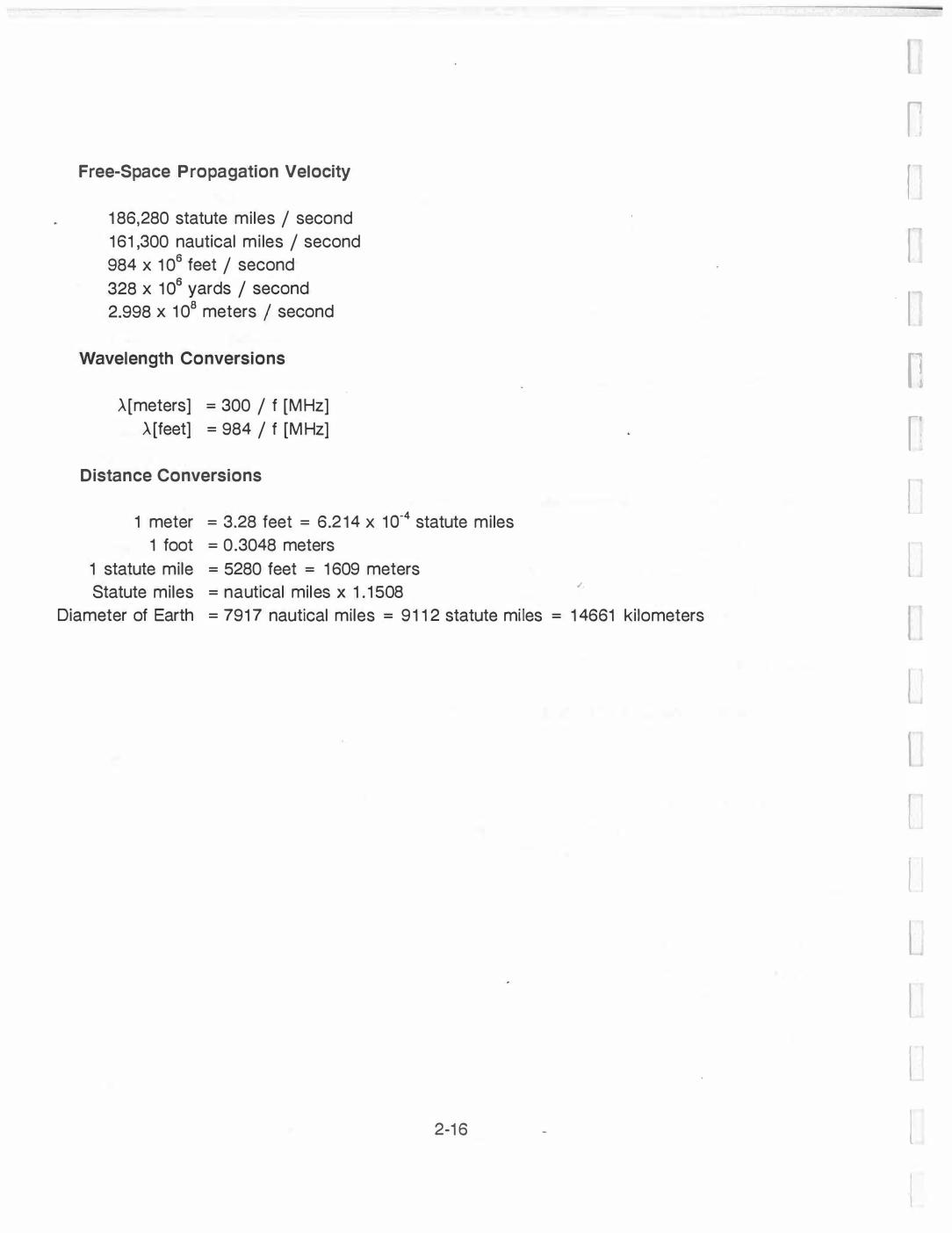
Free-Space Propagation Velocity
1 86,280 statute miles I second 1 61 ,300 nautical mi les I second 984 x 1 06 feet I second 328 x 1 06 yards I second 2.998 x 1 08 meters 1 second
Wavelength Conversions
.A[meters] = 300 I f [MHz] .A [feet] = 984 I f [M Hz]
Distance Conversions
1 meter = 3.28 feet = 6.2 14 x 1 o-4 statute mi les 1 foot = 0.3048 meters
1 statute mile = 5280 feet = 1 609 meters Statute miles = nautical miles x 1 . 1 508
Diameter of Earth = 791 7 nautical miles = 91 1 2 statute mi les = 1 4661 ki lometers
2-1 6
I [ I
I
n n
I
I
l
SECTION 3
COUPLING EQUATIONS
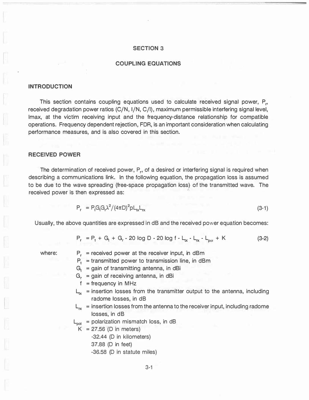
INTRODUCTION
This section contains coupling equations used to calculate received signal power, Pr, received degradation power ratios (C/N , 1/N, C/1) , maximum permissible interfering signal level , lmax, at the victim receiving input and the frequency-distance relationship for compatible operations. Frequency dependent rejection , FOR, is an important consideration when calculating performance measures, and is also covered in this section.
RECEIVED POWER
The determination of received power, Pr, of a desired or interfering signal is required when describing a communications link. In the fol lowing equation, the propagation loss is assumed to be due to the wave spreading (free-space propagation loss) of the transmitted wave. The received power is then expressed as:
�
(3- 1 )
Usually, the above quantities are expressed i n dB and the received power equation becomes:
where:
P = P + G + G - 20 log 0 - 20 log f - ' - L - L + K r t t r "-tx rx pol
Pr = received power at the receiver input, in dBm P1 = transmitted power to transmission l ine, in dBm
Gt = gain of transmitting antenna, in dBi
Gr = gain of receiving antenna, in dBi f = frequency in M Hz
(3-2)
Luc = insertion losses from the transmitter output to the antenna, including radome losses, in dB
Lrx = insertion losses from the antenna to the receiver input, including radome losses, in d B
Lpol = polarization mismatch loss, in dB K = 27.56 (0 in meters)
-32.44 (0 in ki lometers) 37.88 (D in feet) -36.58 (D in statute mi les)
3-1
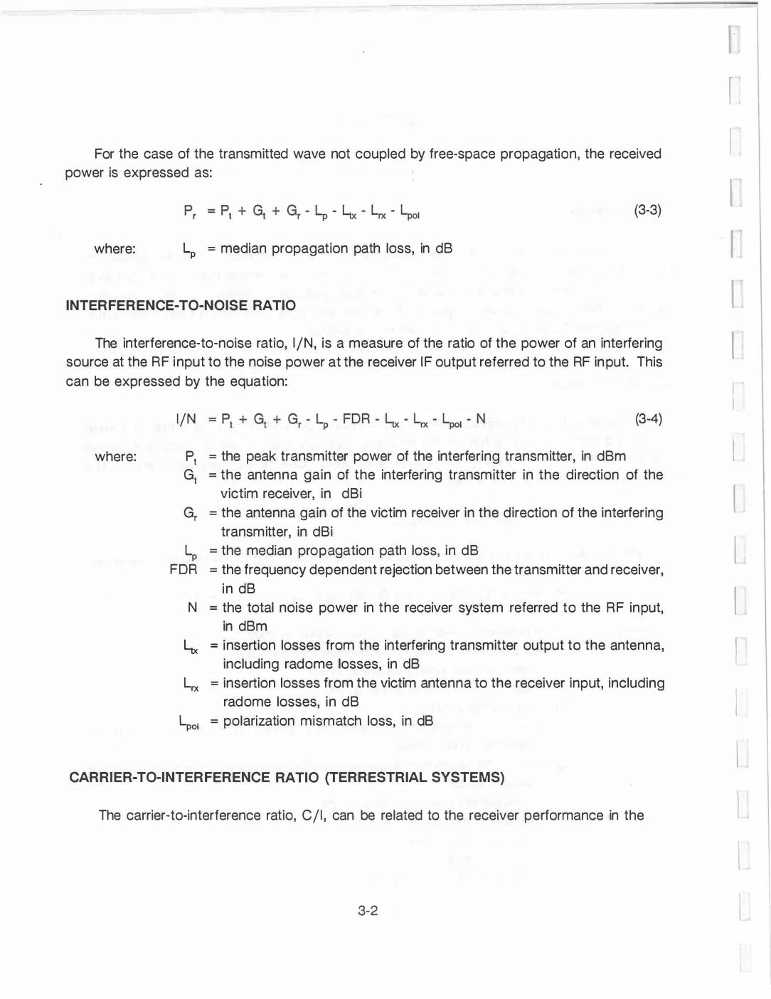
For the case of the transmitted wave not coupled by free-space propagation, the received power is expressed as:
where: LP = median propagation path loss, in dB
(3-3)
INTERFERENCE-TO-NOISE RATIO
The interference-to-noise ratio, 1/N, is a measure of the ratio of the power of an interfering source at the RF input to the noise power at the receiver IF output referred to the RF input. This can be expressed by the equation:
where:
1/N
pt Gt
Gr
LP FOR
N
�
Lrx
(3-4)
= the peak transmitter power of the interfering transmitter, in dBm = the antenna gain of the interfering transmitter in the direction of the
victim receiver, in dBi = the antenna gain of the victim receiver in the direction of the interfering
transmitter, in dBi = the median propagation path loss, in dB = the frequency dependent rejection between the transmitter and receiver,
i n dB = the total noise power in the receiver system referred to the RF input,
in dBm = insertion losses from the interfering transmitter output to the antenna,
including radome losses, in dB = insertion losses from the victim antenna to the receiver input, including
radome losses, in dB
l,01 = polarization mismatch loss, in dB
CARRIER-TO-INTERFERENCE RATIO (TERRESTRIAL SYSTEMS)
The carrier-to-interference ratio, C/1 , can be related to the receiver performance in the
3-2
r
I
[
[
I
[
I
I
[
I
!
I
t
I
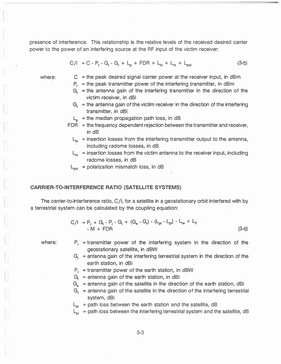
presence of interference. This relationship is the relative levels of the received desired carrier power to the power of an interfering source at the RF input of the victim receiver:
where:
C/1
c
pt Gt
Gr
LP FOR
�
Lrx
(3-5)
= the peak desired signal carrier power at the receiver input, in dBm = the peak transmitter power of the interfering transmitter, in dBm = the antenna gain of the interfering transmitter in the direction of the
victim receiver, in dBi = the antenna gain of the victim receiver in the direction of the interfering
transmitter, in dBi = the median propagation path loss, in dB = the frequency dependent rejection between the transmitter and receiver,
in dB = insertion losses from the interfering transmitter output to the antenna,
including radome losses, in dB = insertion losses from the victim antenna to the receiver input, including
radome losses, in dB Lpo, = polarization mismatch loss, in dB
CARRIER-TO-INTERFERENCE RATIO (SATELLITE SYSTEMS)
The carrier-to-interference ratio, C/1 , for a satel l ite in a geostationary orbit interfered with by a terrestrial system can be calculated by the coupling equation:
where:
C/1 = Pt + Gt - P, - G, + (Ge - Gr) - (�t - �,) - �e + �� - M + FOR (3-6)
P,
G,
pt Gt Ge Gr
�t LP,
= transmitter power of the interfering system in the direction of the geostationary satel l ite, in dBW
= antenna gain of the interfering terrestrial system in the direction of the earth station, in dBi
= transmitter power of the earth station, in dBW = antenna gain of the earth station, in dBi = antenna gain of the satel l ite in the direction of the earth station , dBi = antenna gain of the satel l ite in the direction of the interfering terrestrial
system, dBi = path loss between the earth station and the satel l ite, dB = path loss between the interfering terrestrial system and the satel l ite, dB
3-3

L,e = insertion losses from the earth station transmitter output to the antenna, including radome losses, in dB
L,1 = insertion losses from the interfering transmitter output to the antenna, including radome losses, in dB
M = path loss margin for the earth station signal , dB (assumed to be equal to 1 .2 dB)
FOR = Frequency Dependent Rejection, dB
The maximum differential path loss of two points on the surface of the earth to a satel l ite is 1 .3 dB. This occurs when the potential interferer is directly beneath the satel l ite and the satel l ite earth station is on the horizon. L, - L1 = 1 .0 dB is often used as a more probable value. For the worst case analysis, it could be assumed that the earth station is located at the 3 dB satel l ite beam contour and the radar is at the center beam. Hence,
(3-7)
Substituting equation (3-4) above into (3-3) gives:
(3-8)
CARRIER-TO-NOISE RATIO
The carrier-to-noise ratio, C/N, can be related to the receiver performance in the presence of noise only. The C/N is the relative power levels of desired carrier power at the receiver RF input to the receiver total noise power at the IF output referred to the RF input. This ratio is expressed by the equation:
where: Pt = the peak desired signal transmitter power, in dBm
Gt = the antenna gain of the transmitter, in dBi
Gr = the antenna gain of the receiver antenna, in dBi L, = the median propagation path loss, in dB
(3-9)
� = insertion losses from the transmitter output to the antenna, including radome losses, in dB
� = insertion losses from the antenna to the receiver input, including radome losses, in dB
Lpol = polarization mismatch loss, in dB N = total noise power in the receiver system referred to the RF input, i n dBm
3-4
n
I
r
[
r
I
l
l

MAXIMUM PERMISSIBLE INTERFERENCE LEVEL
For a specified interference-to-noise ratio, 1/N, at the receiver RF input, the maximum permissible interference level, lmax' can be expressed by the equation :
where:
lmax = 1/N + N
lmax = maximum permissible interference level, in dBm 1/N = interference-to-noise ratio, in dB
(3-1 0)
N = total noise power in the receiver system referred to the RF input, in dBm
For a specified C/1 ratio at the receiver RF input, the maximum permissible interference level can be expressed as:
where:
lmax = C - C/1
lmax = maximum interfering level , in dBm C = total power of the transmitted wave, in dB
= total power of the interfering wave, in dB
(3-1 1 )
FREQUENCY-DISTANCE SEPARATION
For an undesired transmitter to be compatible with a receiver, it must be sufficiently separated in distance andjor frequency from the receiver. The frequency andjor distance separation must be sufficient to achieve the loss required to keep the interference below the maximum permissible interference level , lmax. The required loss for compatible operations is given by:
(3-1 2)
where: LP = Median propagation path loss between receiver and interfering source FDR(t.f) = Frequency-dependent rejection, in dB
P1 = Peak transmitter power of the interfering transmitter, in dBm
G1 = Antenna gain of the interfering transmitter in the direction of the victim receiver, in dBi
Gr = Antenna gain of the victim receiver in the direction of the interfering transmitter, in dBi
� = insertion losses from the transmitter output to the antenna, including radome losses, in dB
3-5
Lrx = insertion losses from the antenna to the receiver input, including radome losses, in dB
�01 = polarization mismatch loss, in dB lmax = maximum permissible interference level , in dBm
Once the required loss is calculated , an appropriate propagation and FOR model must be applied to determine the frequency-distance separation relationship.
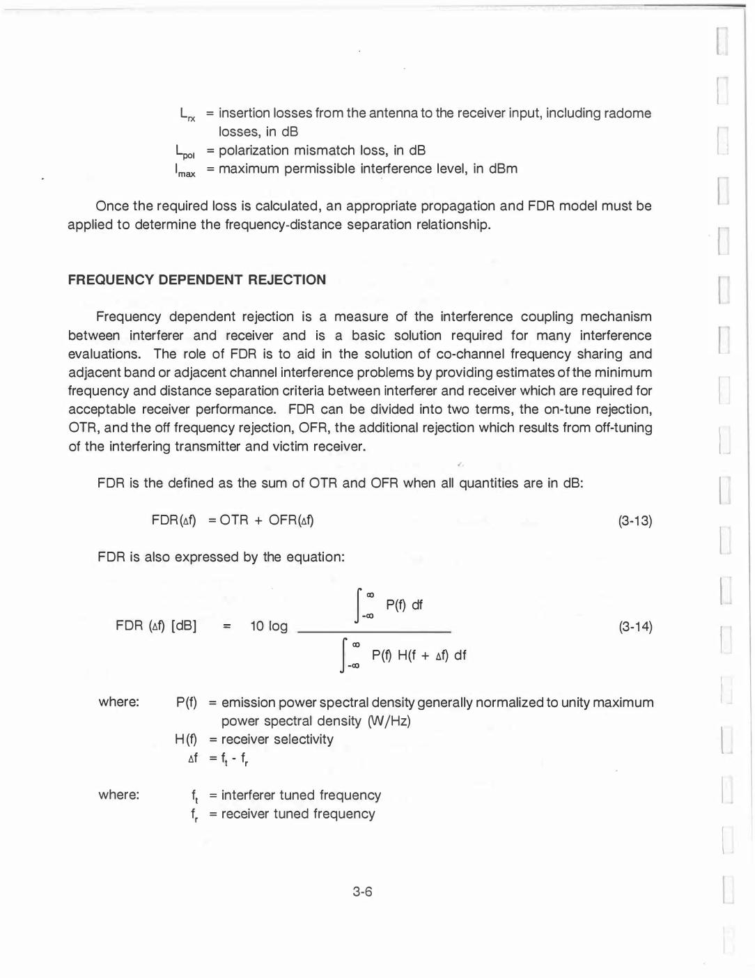
FREQUENCY DEPENDENT REJECTION
Frequency dependent rejection is a measure of the interference coupling mechanism between interferer and receiver and is a basic solution required for many interference evaluations. The role of FOR is to aid in the solution of co-channel frequency sharing and adjacent band or adjacent channel interference problems by providing estimates of the minimum frequency and distance separation criteria between interferer and receiver which are required for acceptable receiver performance. FOR can be divided into two terms, the on-tune rejection, OTR, and the off frequency rejection, OFR, the additional rejection which results from off-tuning of the interfering transmitter and victim receiver.
FOR is the defined as the sum of OTR and OFR when all quantities are in dB:
FOR (Llf} = OTR + OFR(Llf} (3-1 3)
FOR is also expressed by the equation:
FOR (Llf} [dB] - 10 1og
J_: P(f) df
(3-1 4)
J_: P(f) H(f + t.f) df
where: P(f) = emission power spectral density general ly normalized to unity maximum power spectral density 0N /Hz)
where:
H (f) = receiver selectivity Llf = f - f t r
ft = interferer tuned frequency fr = receiver tuned frequency
3-6
I l
I
I
I
[
I
l
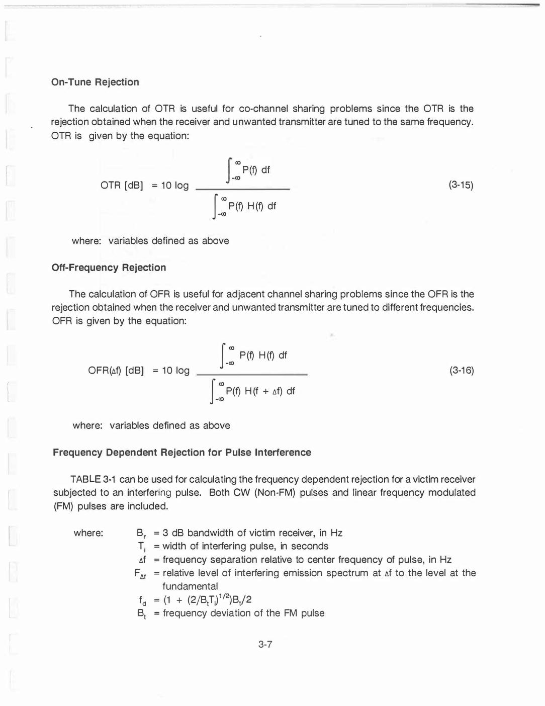
On-Tune Rejection
The calculation of OTR is useful for co-channel sharing problems since the OTR is the rejection obtained when the receiver and unwanted transmitter are tuned to the same frequency. OTR is given by the equation:
OTR [dB] = 1 0 log
J_: P (f) H (f) df
where: variables defined as above
Off-Frequency Rejection
(3-1 5)
The calculation of OFR is useful for adjacent channel sharing problems since the OFR is the rejection obtained when the receiver and unwanted transmitter are tuned to different frequencies. OFR is given by the equation:
OFR(llf) [dB] = 1 0 log
J_: P(f) H (f) df
(3-1 6)
J � P(f) H (f + af) df
where: variables defined as above
Frequency Dependent Rejection for Pulse Interference
TABLE 3-1 can be used for calculating the frequency dependent rejection for a victim receiver subjected to an interfering pulse. Both CW (Non-FM) pulses and l inear frequency modulated (FM) pulses are included.
where: Br = 3 dB bandwidth of victim receiver, in Hz
Ti = width of interfering pulse, in seconds llf = frequency separation relative to center frequency of pulse, in Hz
F t:J.t = relative level of interfering emission spectrum at t:J.f to the level at the fundamental
fd = (1 + (2/B1T1) 1 12)Btf2 B1 = frequency deviation of the FM pulse
3-7

NON-
FM
FM
TABLE 3-1 FREQU ENCY DEPENDENT REJECTION
T ime-Bandwidth
B T . > 1 r 1
B T . < 1 r 1
2 Br T/Bt � 1
B T . > 1 r 1
B/T/Bt < 1
B T . � 1 r 1
Frequency Separat ion
f � 1/ T . + B /2 1 r
f > 1/ T . + B /2 1 r
f = any
f � fd
f > fd
f � fd
f > fd
3-8
FOR
1
2 (BrTi ) FA.f/4
2 (Br\ ) FAf
1
2 Br T /Af/4Bt
2 Br T /Bt
2 8r TiFAf18t
[ [
r I I I l l I
l

r
FORM NTIA-29 (4-80)
U.S. D EPARTMENT OF CO MMERCE NAT1.. TEI.ECOMMUNICATIONS ANO INFORMATION AOMIN ISTRATION
BI B LIOGRAPHIC OAT A SHEET
1 . PUBLICATION NO. 2. Gov·t Accession No. 3. Recipienrs Accession No.
NTIA TN 89-2
4. TITLE AND SUBTITLE
SPECTRUM MANAGEM ENT TECHNICAL HANDBOOK
7 . AUTHOR(S)
8. PERFORMING ORGANIZATION NAME AND ADDRESS
National Telecommunications and Information Admin istration
1 79 Admiral Cochrane Drive Annapolis, Maryland 21 401
1 1 . Sponsoring Organization Name and Address
U.S. Department of CommercejNTIA 1 79 Admiral Cochrane Drive Annapolis, Maryland 2 1401
14. SUPPLEMENTARY NOTES
6. Performing Organization Code
9. Project/Task/Work Unit No.
901 9 1 71
10. Contract/Grant No.
1 2 . Type of Repon and Period Covered
Technical Note
1 3 .
1 5 . ABSTRACT ( A 200-word o r le� factual summary of most significant information. If document includes a significant bibliography o r literature survey, mention it here.)
This handbook is a compilation of the procedures, definitions, relationships and conversions essential to electromagnetic compatibi l ity analysis. It is intended as a reference for NTIA engineers.
16. Key Words (A lphabetical order. separated b y semicolons}
Conversion Factors; Coupling Equations; Definitions; Techn ical Relationships
1 7 . AVA ILABILITY STATEMENT 1 8 . Security Class. ( This report} 20. Number of pages
UNCLASSIF IED 48 FOR INTERNAL D ISTRIBUTION 19. Security Class. ( This page J 2 1 . Price:
UNCLASSIFI ED
g U.S. Govemmenl PrinttnQ Office: t98o--878·•95/529