spectral methods for uncertainty quantification · the focus is on spectral methods and especially...
TRANSCRIPT

Spectral Methods for UncertaintyQuantication
Emil Brandt Kærgaard
Kongens Lyngby 2013
IMM-M.Sc.-2013-0503

Technical University of Denmark
Department of Applied Mathematics and Computer Science
Building 303B, DK-2800 Kongens Lyngby, Denmark
www.compute.dtu.dk IMM-M.Sc.-2013-0503
Summary (English)
This thesis has investigated the eld of Uncertainty Quantication with regardto dierential equations. The focus is on spectral methods and especially thestochastic Collocation method. Numerical tests are conducted and the stochas-tic Collocation method for multivariate problems is investigated. The Smolyaksparse grid method is applied in combination with the stochastic Collocationmethod on two multivariate stochastic dierential equations. The numericaltests showed that the sparse grids can reduce the computational eort and atthe same time produce very accurate results.
The rst part of the thesis introduces the mathematical background for work-ing with Uncertainty Quantication, the theoretical background for generalizedPolynomial Chaos and the three methods for the Uncertainty Quantication.These methods are the Monte Carlo sampling, the stochastic Galerkin methodand the stochastic Collocation method.The three methods have been tested numerically on the univariate stochasticTest equation to test accuracy and eciency and further numerical tests of theGalerkin method and the Collocation method have been conducted with regardto the univariate stochastic Burgers' equation. The numerical tests have beencarried out in Matlab.
The last part of the thesis involves an introduction of the multivariate stochas-tic Collocation method and numerical tests. Furthermore a few methods forreducing the computational eort in high dimensions is introduced. One ofthese methods - the Smolyak sparse grids - is applied together with the stochas-tic Collocation method on the multivariate Test equation and the multivariateBurgers' equation. This resulted in accurate and ecient estimates of the statis-

ii
tics.

Summary (Danish)
Denne afhandling undersøger og anvender metoder til kvanticering af usikker-hed. Fokus i opgaven har været at undersøge spektrale metoder til usikkerheds-bestemmelse med særligt fokus på den stokastiske Collocation metode. Der erforetaget numeriske undersøgelser af metoderne og den stokastiske Collocationmetode er blevet afprøvet på multivariate problemer. Den stokastiske Colloca-tion metode er desuden blevet testet sammen med Smolyak sparse grids på tomultivariate dierentialligninger hvilket var en klar eektivisering og førte tilnøjagtige resultater.
Den første del af afhandlingen introducerer den matematiske baggrund for at ar-bejde med emnet og en teoretisk introduktion af generaliseret Polynomial Chaosog de tre metoder til usikkerhedsbestemmelse. De anvendte metoder er MonteCarlo Sampling, den stokastiske Galerkin metode og den stokastiske Collocationmetode.Der er foretaget numeriske test med de tre metoder på den univariate Testequation for at undersøge eektivitet og nøjagtighed. Desuden er der foretagetyderligere numeriske undersøgelser af Galerkin metoden og Collocation metodenpå den univariate stokastiske Burgers' equation. De numeriske test er foretageti Matlab.
Den sidste del af afhandlingen omhandler introduktion og afprøvning af denmultivariate stokastiske Collocation metode. Der bliver også introduceret eremetoder til at reducere den beregningsmæssige byrde der opstår når antallet afdimensioner øges. En af disse metoder kaldes Smolyak sparse grid metoden ogdenne er blevet anvendt sammen med den stokastiske Collocation metode påden multivariate Test equation og den multivariate Burgers' equation, hvilket

iv
førte til gode resultater.

Preface
This thesis was prepared at DTU Compute: Department of Applied Mathemat-ics and Computer Science at the Technical University of Denmark in fullmentof the requirements for acquiring an M.Sc. in Mathematical Modelling andComputing. The thesis was carried out in the period from December 3rd 2012to May 3rd 2013 with associate Professor Allan P. Ensig-Karup as supervisor.
The thesis deals with spectral methods for Uncertainty Quantication and in-troduces a method to decrease the computational eort of these methods in highdimensions.The thesis consists of a study of methods for Uncertainty Quantication andthe application of these. The focus has been on conducting Uncertainty Quan-tication for dierential equations and using spectral methods to investigate theuncertainty. Especially the stochastic Collocation method has been investigatedand the use of this method in more than one dimension.
The thesis is written to a reader that has basic knowledge of mathematicalmodelling and mathematics. It is furthermore assumed that the reader hasknowledge of Matlab and of numerical tools for solving dierential equations.
Lyngby, 03-May-2013
Emil Brandt Kærgaard

vi

Acknowledgements
I would like to thank my supervisor, Associate Professor Allan P. Ensig-Karup,and Ph.D. student Daniele Bigoni for help, advice and inspiration during theproject. They have provided guidance and advice through the project wheneverI asked for it.
Another person who deserves thanks is Emil Kjær Nielsen who has been explor-ing this interesting topic alongside me. We have had some great conversationsand discussions and I really appreciate his inputs and his humor.
Furthermore I would like to thank Signe Søndergaard Jeppesen for her moralesupport and for listening when I needed it.
Last but not least I would like to thank Emil Schultz Christensen and KristianRye Jensen for their readiness to help, their advice and their support.

viii
Contents
Summary (English) i
Summary (Danish) iii
Preface v
Acknowledgements vii
1 Introduction 11.1 Uncertainty Quantication . . . . . . . . . . . . . . . . . . . . . . 21.2 Motivation and goals for the thesis . . . . . . . . . . . . . . . . . 31.3 Basic literature . . . . . . . . . . . . . . . . . . . . . . . . . . . . 41.4 Outline of thesis . . . . . . . . . . . . . . . . . . . . . . . . . . . 4
2 Mathematical background 72.1 Hilbert space and inner products . . . . . . . . . . . . . . . . . . 72.2 Orthogonal Polynomials . . . . . . . . . . . . . . . . . . . . . . . 8
2.2.1 Three-term Recurrence relation . . . . . . . . . . . . . . . 92.2.2 Example: Hermite Polynomials . . . . . . . . . . . . . . . 92.2.3 Example: Jacobi polynomials . . . . . . . . . . . . . . . . 112.2.4 Example: Legendre Polynomials . . . . . . . . . . . . . . 12
2.3 Gauss Quadrature . . . . . . . . . . . . . . . . . . . . . . . . . . 142.3.1 Computing nodes and weights for Gauss Quadrature . . . 142.3.2 Example: Gauss Hermite Quadrature . . . . . . . . . . . 152.3.3 Gauss-Lobatto Quadrature . . . . . . . . . . . . . . . . . 17
2.4 Polynomial Interpolation . . . . . . . . . . . . . . . . . . . . . . . 182.4.1 Relationship between nodal and modal representations . . 19
2.5 Spectral methods . . . . . . . . . . . . . . . . . . . . . . . . . . . 202.6 Numerical solvers . . . . . . . . . . . . . . . . . . . . . . . . . . . 20

x CONTENTS
2.6.1 Solver for dierential equations in space . . . . . . . . . . 202.6.2 Solvers for time dependent problems . . . . . . . . . . . . 24
3 Basic concepts within Probability Theory 273.1 Distributions and statistics . . . . . . . . . . . . . . . . . . . . . 27
3.1.1 Example: Gaussian distribution . . . . . . . . . . . . . . . 283.1.2 Example: Uniform distribution . . . . . . . . . . . . . . . 293.1.3 Multiple dimensions . . . . . . . . . . . . . . . . . . . . . 303.1.4 Statistics . . . . . . . . . . . . . . . . . . . . . . . . . . . 313.1.5 Inner product and statistics . . . . . . . . . . . . . . . . . 31
3.2 Input parameterizations . . . . . . . . . . . . . . . . . . . . . . . 32
4 Generalized Polynomial Chaos 334.1 Generalized Polynomial Chaos in one dimension . . . . . . . . . . 344.2 Multivariate Generalized Polynomial Chaos . . . . . . . . . . . . 344.3 Statistics for gPC expansions . . . . . . . . . . . . . . . . . . . . 36
5 Stochastic Spectral Methods 395.1 Non-intrusive methods . . . . . . . . . . . . . . . . . . . . . . . . 40
5.1.1 Monte Carlo Sampling . . . . . . . . . . . . . . . . . . . . 405.1.2 Stochastic Collocation Method . . . . . . . . . . . . . . . 41
5.2 Intrusive methods . . . . . . . . . . . . . . . . . . . . . . . . . . 435.2.1 Stochastic Galerkin method . . . . . . . . . . . . . . . . . 43
6 Test problems 476.1 Test Equation . . . . . . . . . . . . . . . . . . . . . . . . . . . . . 47
6.1.1 Normal distributed parameters . . . . . . . . . . . . . . . 486.1.2 Uniform distributed parameters . . . . . . . . . . . . . . . 516.1.3 Multivariate Test Equation . . . . . . . . . . . . . . . . . 53
6.2 Burgers' Equation . . . . . . . . . . . . . . . . . . . . . . . . . . 55
7 Test of UQ methods on the Test Equation 597.1 Monte Carlo Sampling . . . . . . . . . . . . . . . . . . . . . . . . 59
7.1.1 Gaussian distributed α-parameter . . . . . . . . . . . . . 607.1.2 Uniformly distributed α-parameter . . . . . . . . . . . . . 63
7.2 Stochastic Collocation Method . . . . . . . . . . . . . . . . . . . 647.2.1 Implementation . . . . . . . . . . . . . . . . . . . . . . . . 657.2.2 Gaussian distributed α-parameter . . . . . . . . . . . . . 667.2.3 Uniformly distributed α-parameter . . . . . . . . . . . . . 67
7.3 Stochastic Galerkin Method . . . . . . . . . . . . . . . . . . . . . 697.3.1 Implementation . . . . . . . . . . . . . . . . . . . . . . . . 707.3.2 Gaussian distributed α-parameter . . . . . . . . . . . . . 717.3.3 Uniformly distributed α-parameter . . . . . . . . . . . . . 72
7.4 Conclusion . . . . . . . . . . . . . . . . . . . . . . . . . . . . . . 73

CONTENTS xi
8 Burgers' Equation 758.1 Stochastic gPC Galerkin method . . . . . . . . . . . . . . . . . . 75
8.1.1 Numerical approximations . . . . . . . . . . . . . . . . . . 778.1.2 Implementation . . . . . . . . . . . . . . . . . . . . . . . . 798.1.3 Numerical experiments . . . . . . . . . . . . . . . . . . . . 80
8.2 Stochastic Collocation Method . . . . . . . . . . . . . . . . . . . 818.2.1 Implementations . . . . . . . . . . . . . . . . . . . . . . . 838.2.2 Numerical experiments . . . . . . . . . . . . . . . . . . . . 84
9 Discussion: Choice of method 87
10 Literature Study 8910.1 Brief Introduction to topics and articles . . . . . . . . . . . . . . 8910.2 Sparse Pseudospectral Approximation Method . . . . . . . . . . 90
10.2.1 Introduction of notation and concepts . . . . . . . . . . . 9110.2.2 Overall approach . . . . . . . . . . . . . . . . . . . . . . . 9210.2.3 Further reading . . . . . . . . . . . . . . . . . . . . . . . . 93
10.3 Compressive sampling: Non-adapted sparse approximation of PDES 9310.3.1 Overall approach . . . . . . . . . . . . . . . . . . . . . . . 9310.3.2 Recoverability . . . . . . . . . . . . . . . . . . . . . . . . . 9510.3.3 Further reading . . . . . . . . . . . . . . . . . . . . . . . . 96
11 Multivariate Collocation Method 9711.1 Tensor Product Collocation . . . . . . . . . . . . . . . . . . . . . 9711.2 Multivariate expansions and statistics . . . . . . . . . . . . . . . 9811.3 Smolyak Sparse Grid Collocation . . . . . . . . . . . . . . . . . . 100
11.3.1 Clenshaw-Curtis: Nested sparse grid . . . . . . . . . . . . 101
12 Numerical tests for multivariate stochastic PDEs 10312.1 Test Equation with two random variables . . . . . . . . . . . . . 103
12.1.1 Implementation . . . . . . . . . . . . . . . . . . . . . . . . 10412.1.2 Gaussian distributed α-parameter and initial condition β 10512.1.3 Gaussian distributed α and uniformly distributed initial
condition β. . . . . . . . . . . . . . . . . . . . . . . . . . . 10812.2 Multivariate Burgers' Equation . . . . . . . . . . . . . . . . . . . 111
12.2.1 Burgers' Equation with stochastic boundary conditions . 11112.2.2 3-variate Burgers' equation . . . . . . . . . . . . . . . . . 115
13 Tests with Smolyak sparse grids 12313.1 Introduction of the sparse grids . . . . . . . . . . . . . . . . . . . 124
13.1.1 Sparse Gauss Legendre grid . . . . . . . . . . . . . . . . . 12413.2 Sparse Clenshaw-Curtis grid . . . . . . . . . . . . . . . . . . . . . 12513.3 Smolyak sparse grid applied . . . . . . . . . . . . . . . . . . . . . 127
13.3.1 The 2-variate Test Equation . . . . . . . . . . . . . . . . . 127

xii CONTENTS
13.3.2 The 2-variate Burgers' Equation . . . . . . . . . . . . . . 13213.4 Conclusion . . . . . . . . . . . . . . . . . . . . . . . . . . . . . . 135
14 Discussion 13714.1 Future work . . . . . . . . . . . . . . . . . . . . . . . . . . . . . . 138
15 Conclusion 141
A Supplement to the mathematical background 143A.1 Orthogonal Polynomials . . . . . . . . . . . . . . . . . . . . . . . 143
A.1.1 Alternative denition of the Hermite polynomials . . . . . 143A.2 Probability theory . . . . . . . . . . . . . . . . . . . . . . . . . . 144A.3 Random elds and useful spaces . . . . . . . . . . . . . . . . . . 144A.4 Convergence and Central Limit Theorem . . . . . . . . . . . . . . 145A.5 Introduction of strong and weak gPC approximation . . . . . . . 146
A.5.1 Strong gPC approximation . . . . . . . . . . . . . . . . . 146A.5.2 Weak gPC approximation . . . . . . . . . . . . . . . . . . 147
B Matlab 151B.1 Toolbox . . . . . . . . . . . . . . . . . . . . . . . . . . . . . . . . 151
B.1.1 Polynomials and quadratures . . . . . . . . . . . . . . . . 151B.1.2 Vandermonde-like matrices. . . . . . . . . . . . . . . . . . 167B.1.3 ERK . . . . . . . . . . . . . . . . . . . . . . . . . . . . . . 168
B.2 Test Equation . . . . . . . . . . . . . . . . . . . . . . . . . . . . . 168B.2.1 Monte Carlo . . . . . . . . . . . . . . . . . . . . . . . . . 168B.2.2 Stochastic Collocation Method . . . . . . . . . . . . . . . 175B.2.3 Stochastic Galerkin method . . . . . . . . . . . . . . . . . 179
B.3 Burgers' Equation . . . . . . . . . . . . . . . . . . . . . . . . . . 184B.3.1 Stochastic Collocation Method . . . . . . . . . . . . . . . 184B.3.2 Stochastic Galerkin method . . . . . . . . . . . . . . . . . 189
B.4 Burgers' Equation 2D . . . . . . . . . . . . . . . . . . . . . . . . 189B.5 Burgers' Equation 3D . . . . . . . . . . . . . . . . . . . . . . . . 193B.6 Numerical tests with sparse grids . . . . . . . . . . . . . . . . . . 199
B.6.1 Numerical tests for the multivariate Test equation . . . . 199B.6.2 Numerical tests for the multivariate Burgers' equation . . 208
Bibliography 211

Chapter 1
Introduction
The elds of numerical analysis and scientic computing have been in great de-velopment the last couple of decades. The introduction of ecient computershas lead to massive use of mathematical models and extensive research havebeen conducted to optimize the use of these models.A topic of great interest is the errors in the numerical results and it is currently aeld of active research. This has lead to an increased knowledge within the eldand many improvements have been obtained. In general the errors of numericalanalysis is classied into three groups [16]: Model errors, numerical errors anddata errors.
The model errors arises when the applied mathematical model does not describea given problem exactly. This type of errors will almost always be present whendescribing real life problems since the applied mathematical models are simpli-cations of the problem and since they are based on a set of assumptions.Numerical errors arises when the mathematical models are solved numerically.The numerical methods usually involves approximations of the exact model so-lutions and even though these approximations can be improved by using theoryabout convergence and stability, the errors will still be there due to the niteprecision on computers.The data errors refers to the uncertainty in the input to the mathematical modelswhich propagates through the model to the output. These errors are unavoid-

2 Introduction
able when the input data is measurement data, since measurements will alwayscontain errors. Errors in the input also arise when there is limited knowledgeabout the input variables or parameters.
1.1 Uncertainty Quantication
As outlined here there are lots of errors to investigate when working with nu-merical analysis. The focus in this thesis is on quantifying the uncertainty thatpropagates from the input to a mathematical model to the output. It is a eldof very active research and many dierent approaches are applied in order tooptimize the quantication of the uncertainty. In this thesis the focus will beon a class of methods that are known as spectral methods and on quantify-ing uncertainty in stochastic dierential equations. An example is the ordinarydierential equation called the Test equation which is formulated as
d
dtu(t) = −λu(t), u(0) = b.
By introducing uncertainty in the λ-parameter the solutions to the Test equationbased dierent realizations of the stochastic λ-parameter will vary a lot. In gure1.1 9 of such solutions are plotted and it is seen that there is a lot of variationin the solutions and the uncertainty is increased with time. The 9 solutions ingure 1.1 are plotted in the timespan [0, 1] but if the timespan was increased toe.g. [0, 2] the dierence in the solutions would have been even greater. In factthe uncertainty grows exponentially with time. This is a very good reason forapplying uncertainty quantication.
0 0.5 1
1
2
t
Solutions
Figure 1.1: 9 deterministic solutions to the stochastic Test equation

1.2 Motivation and goals for the thesis 3
In this thesis three methods will be used for conducting uncertainty quantica-tion. One of them is the Monte Carlo Sampling which is a brute force methodthat based on a large number of samples approximates the statistics of thestochastic solutions. The samples refers solutions to the stochastic problemwhich are obtained by solving the system deterministically for a set of realiza-tions of the stochastic inputs.The two other methods are spectral methods which are based on using orthog-onal polynomials to represent the stochastic solution of the problem at hand.The two methods are called the stochastic Collocation method and the stochas-tic Galerkin method. The stochastic Collocation method does in general notrequire many implementations of a solver for the deterministic problem is avail-able.The stochastic Galerkin method often requires analytical derivations and newimplementations. But it is usually obtains more accurate results than thestochastic Collcation method so both methods have strengths and weaknesses.
1.2 Motivation and goals for the thesis
The combination of spectral methods and uncertainty quantication is a eld ofstudy which is in great development these years and a lot of research is currentlygoing on worldwide. Besides this the uncertainty quantication has become animportant numerical tool that is applied in many companies.The studies within the eld of uncertainty quantication involves many dierenttopics and approaches. One topic that has received a lot of attention recentlyis how to reduce the computational eort when applying spectral methods suchas stochastic Collocation method to multivariate problems.Because of the rapid development within uncertainty quantication this thesisincludes a section that introduces a few interesting approaches to decrease thecomputational eort based on a literature study of recent scientic articles.
The overall goal of the thesis is to investigate the eld of uncertainty quanti-cation and gain an insight in the topic. The focus is the combination of spectralmethods and uncertainty quantication.This means that the thesis will include an introduction to some of the necessarytheory for investigating the eld and then introduce several uncertainty quan-tication methods which involve at least one intrusive and one non-instrusivemethod. The goal of the thesis is to introduce the methods theoretically andconduct numerical tests.The focus of the thesis is to introduce the topic and to apply spectral methodsfor uncertainty quantication. The spectral methods for uncertainty quanti-
4 Introduction
cation are attractive in many ways but the computational eort of the methodsoften grows rapidly in multivariate problems. It is therefore a goal of the thesisto apply at least one method to reduce the computational eort.It is a choice not to investigate more advanced PDEs and instead include a moreadvanced setting where the computational eort is sought to be reduced.
It is a choice not to investigate more advanced PDEs and instead include a moreadvanced setting where the computational eort is sought to be reduced.
1.3 Basic literature
The book Numerical methods for stochastic computations: a spectral methodapproach by Dongbin Xiu has served as a basis for working with uncertaintyquantication and the book Spectral Methods for Uncertainty Quantication byO. Le Maitre and O. Knio has been used as a reference.Furthermore the article Gaussian Quadrature and the Eigenvalue Problem byJohn A. Gubner has been used as a basis for some of the mathematical back-ground.
1.4 Outline of thesis
This thesis has a focus on spectral methods for uncertainty quantication andincludes theoretical and numerical applications of such.In Chapter 2 the mathematical background is outlined. This includes orthogonalpolynomials, quadratures rules and numerical tools. The mathematical intro-duction is continued in Chapter 3 which contains some basic concepts withinprobability theory. These two chapters also serves as an introduction to thenotation that is used throughout the thesis.Chapter 4 gives an introduction to generalized Polynomial Chaos (gPC), thegPC expansions and the the important properties of gPC. The generalized Poly-nomial Chaos serves as a basis for introducing the stochastic Galerkin methodand the stochastic Collocation method in chapter 5. The theoretical backgroundfor applying these two methods is outlined in this chapter and the chapter servesas a basis for conducting numerical tests. Chapter 6 introduces an ordinary dif-ferential equation (ODE) denoted the Test Equation and a partial dierentialequation (PDE) called Burgers' Equation. These two dierential equations willform the basis of the numerical tests.

1.4 Outline of thesis 5
In chapter 7 numerical tests of the univariate Test equation is conducted and theaccuracy and convergence of the uncertainty quantication methods and chap-ter 8 contains numerical tests involving Burgers' equation. The numerical testsof the uncertainty quantication methods has conrmed some of the propertiesoutlined in the theory and Chapter 9 gives a brief summery of the strengths andweaknesses for methods and outline which method that will be use in the restof the thesis.Chapter 10 is a literature study which describes some interesting topics whichare recently introduced in the eld of uncertainty quantication. Chapter 11introduces the multivariate stochastic collocation method. The multivariatestochastic Collocation method is investigated in Chapter 12 through numericaltests and in chapter 13 the Smolyak sparse grids are applied in combinationwith the multivariate stochastic Collocation method.Chapter 14 is a discussion of the methods and the conducted numerical tests.It includes a section which outline some possible future works.

6 Introduction

Chapter 2
Mathematical background
The uncertainty quantication conducted in this thesis is based on theory withinmany elds. The two main elds of mathematics are probability theory and thetheory regarding spectral methods.In this chapter the basic tools for applying spectral methods are outlined as wellas the numerical solvers for deterministic partial dierential equations (PDE)used in this thesis.In chapter 3 the stochastic theory will be outlined. This means that unlessanything else is stated the theory outlined in this chapter is deterministic.
2.1 Hilbert space and inner products
Before the theory of spectral methods can be outlined some basic denitions areneeded which will be introduced here. First of all L2 denotes a Hilbert spacewith a corresponding inner product and its induced norm. The L2 space is de-
ned such that for u ∈ L2 it holds that ‖u‖2 =(∫S|u|2dµ
) 12 <∞ where µ is a
Lebesgue measure and S is the support of the measure.The measure µ is in this thesis used such that the integral
∫Df(x)dµ(x) can
be replaced by the weighted integral∫Df(x)w(x)dx with w(x) = 0 for x out-
side the domain D. Furthermore the following denition will be used µ(R) =

8 Mathematical background
∫∞−∞ w(x)dx. The general measure theory is beyond the scope of this thesis andthe interested reader can see e.g. [16] or [19] for an introduction.The inner products in this thesis will be dened as
〈u, v〉 =
∫S
u(x)v(x)dµ(x) =
∫S
u(x)v(x)w(x)dx. (2.1)
The inner product is actually a weighted inner product and is generally referredto as 〈·, ·〉w but in this thesis the notation 〈·, ·〉 is used for simplicity. Theweighted Hilbert space L2
w[a, b] can be formulated as
L2w[a, b] = u : [a, b]→ R |
∫ b
a
u2(x)dµ(x) =
∫ b
a
u2(x)w(x)dx <∞.
Furthermore a stochastic Hilbert space is used later on and it is dened as
L2dFZ (IZ) = f : IZ → R |E[f2(Z)] =
∫IZ
f2(z)dFZ(z) <∞, (2.2)
where Z is a stochastic variable.
2.2 Orthogonal Polynomials
In this section a basic introduction to the theory of orthogonal polynomials isgiven and further information can be found in e.g. [1]. In the following N willbe used as either N = N0 = 0, 1, 2, . . . or as an index set N = 0, 1, . . . , N.There are many dierent notations for an orthogonal polynomial and in thisproject the following will be adopted
Φn(x) = anxn + an−1x
n−1 + · · ·+ a1x1 + a0, an 6= 0, (2.3)
where the leading coecient, an, is non-zero. Often the orthogonal polynomialsare referred to in monic form which means that the leading coecient is one.Since the leading coecient is non-zero a transformation of the general form(2.3) into monic form is made by dividing with an
Pn(x) =Φn(x)
an= xn +
an−1
anxn−1 + · · ·+ a1
anx1 +
a0
an, an 6= 0.
Another often used representation of the orthogonal polynomial which is intro-duced in e.g. [10] yields
φn(x) = xn +
n−1∑k=0
〈xn, φk(x)〉〈φk(x), φk(x)〉
φk(x), n ≥ 1.

2.2 Orthogonal Polynomials 9
When a system of polynomials Φn(x)n∈N fulls (2.4) it is said to be orthogonalwith respect to a real positive measure µ.∫
S
Φn(x)Φm(x)dµ(x) = γnδn,m, n,m ∈ N, (2.4)
where S is the support of the measure µ, δn,m is the Kronecker delta functionand γn is a normalization constant dened as
∫S
Φ2n(x)dµ(x) = γn for n ∈ N.
As described in the previous section the measure µ typically has a density w(x)which means that the integral (2.4) could be formulated as∫
S
Φn(x)Φm(x)w(x)dx = γnδnm, n,m ∈ N.
An orthonormal system of polynomials refers to a system of orthogonal polyno-mials which have normalization constants 1. To normalize a set of orthogonalpolynomials the individual polynomials are divided by the corresponding nor-
malization factors, i.e. Φn(x) = Φn(x)√γn
.
2.2.1 Three-term Recurrence relation
A general three-term recurrence relation can be formulated for Φn(x) with x ∈ Rand states
−xΦn(x) = βnΦn+1(x) + αnΦn(x) + γnΦn−1(x), n ≥ 1,
where βn, γn 6= 0 and γnβn−1
> 0 as introduced in [19]. Equivalently a three-term
recurrence relation can be established for φn(x) in monic form which yields
φn+1(x) = (x− an)φn(x)− bnφn−1(x), n ≥ 1, (2.5)
where an = 〈xφn(x),φn(x)〉
〈φn(x),φn(x)〉
bn = 〈φn(x),xφn−1(x)〉〈φn−1(x),φn−1(x)〉 = 〈φn(x),φn(x)〉
〈φn−1(x),φn−1(x)〉 ≥ 0
For more information on the three-term recurrences see [10] and [19].
2.2.2 Example: Hermite Polynomials
The Hermite Polynomials is an important class of polynomials and there aretwo often used denitions of the polynomials. Both are introduced in this thesis
10 Mathematical background
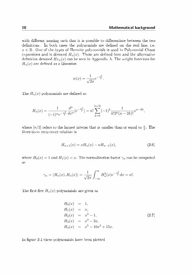
with dierent naming such that it is possible to dierentiate between the twodenitions. In both cases the polynomials are dened on the real line, i.e.x ∈ R. One of the types of Hermite polynomials is used in Polynomial Chaosexpansions and is denoted Hn(x). These are dened here and the alternativedenition denoted Hen(x) can be seen in Appendix A. The weight functions forHn(x) are dened as a Gaussian
w(x) =1√2πe−
x2
2 .
The Hn(x) polynomials are dened as
Hn(x) =1
(−1)ne−x2
2
dn
dxn[e−
x2
2 ] = n!
[n/2]∑k=0
(−1)k1
k!2k(n− 2k)!xn−2k,
where [n/2] refers to the largest integer that is smaller than or equal to n2 . The
three-term recurrence relation is
Hn+1(x) = xHn(x)− nHn−1(x), (2.6)
where H0(x) = 1 and H1(x) = x. The normalization factor γn can be computedas
γn = 〈Hn(x), Hn(x)〉 =1√2π
∫ ∞−∞
H2n(x)e−
x2
2 dx = n!.
The rst ve Hn(x) polynomials are given as
H0(x) = 1,
H1(x) = x,
H2(x) = x2 − 1, (2.7)
H3(x) = x3 − 3x,
H4(x) = x5 − 10x3 + 15x.
In gure 2.1 these polynomials have been plotted

2.2 Orthogonal Polynomials 11
−3 −2 −1 0 1 2 3
−5
0
5
x
Hn(x
)
H0(x)
H1(x)
H2(x)
H3(x)
H4(x)
Figure 2.1: The rst ve Hermite polynomials.
The intuitive inspection of gure 2.1 seems to justify the implementation of thepolynomials given in appendix B since the plotted polynomials are of the rightorder. They also ts very well with the analytical expressions for the rst vepolynomials given in (2.7) and resembles the gures in [16] and [19].
2.2.3 Example: Jacobi polynomials
The Jacobi polynomials are a widely used class of polynomials and they aredened as the eigenfunctions for a certain Sturm-Liouville problem which willnot be described further here. A more in-depth description of the origin of theJacobi Polynomials is found in [15].The Jacobi polynomials, Pα,βn , can be described by the following three-termrecurrence relation
aα,βn+1,nPα,βn+1(x) = (aα,βn,n + x)Pα,βn (x)− aα,βn−1,nP
α,βn−1(x), (2.8)
where the rst two polynomials are given by
Pα,β0 (x) = 1
Pα,β1 (x) =1
2(α− β + (α+ β + 2)x)

12 Mathematical background
and the coecient for n = 0 is aα,β−1,0 = 0 and for n > 0 the coecients are
aα,βn−1,n = 2(n+α)(n+β)(2n+α+β+1)(2n+α+β)
aα,βn,n = α2−β2
(2n+α+β+2)(2n+α+β)
aα,βn+1,n = 2(n+1)(n+α+β+1)(2n+α+β+2)(2n+α+β+1) .
The weight function for the Jacobi polynomials is w(x) = (1− x)α(1 + x)β andthe normalization constant is given by
γα,βn = ||Pα,βn ||2J = 2α+β+1 (n+ α)!(n+ β)!
n!(2n+ α+ β)(n+ α+ β)!,
where ‖ · ‖J = ‖ · ‖L2w[−1,1] is the norm which belongs to the space of Jacobi
polynomials.
2.2.4 Example: Legendre Polynomials
The Legendre polynomials are a subclass of the Jacobi polynomials with α =β = 0 and weight w = 1 and they will be used extensively in this thesis.The Legendre polynomials Ln(x) ∈ [−1, 1] are usually normalized such thatLn(1) = 1 and in this normalized form the polynomials can be formulated as
Ln(x) =1
2n
[n2 ]∑k=0
(−1)k(nk
)(2n− 2k
n
)xn−2k, (2.9)
where [n2 ] denote n2 rounded down to nearest integer. For the weight function
w(x) the Legendre polynomials are an orthogonal basis for L2w[−1, 1]. The rst
two Legendre polynomials are L0(x) = 1 and L1(x) = x and the three-termrecurrence relation is
(n+ 1)Ln+1(x) = (2n+ 1)xLn(x)− nLn−1(x). (2.10)
It is often written in monic form as well which yields
Ln+1(x) =2n+ 1
n+ 1xLn(x)− n
n+ 1Ln−1(x). (2.11)
With the denition (2.11) of the Legendre pPolynomials the normalization con-stant γn can be computed as
γn = 〈Ln, Ln〉 =
∫ 1
−1
L2n(x)w(x)dx =
1
2n+ 1.

2.2 Orthogonal Polynomials 13
The rst ve Legendre polynomials are given by
L0(x) = 1,
L1(x) = x,
L2(x) =1
2(3x2 − 1), (2.12)
L3(x) =1
2(5x3 − 3x),
L4(x) =1
8(35x4 − 30x2 + 3),
(2.13)
The polynomials have been plotted in gure 2.2.
−3 −2 −1 0 1 2 3
−1
−0.5
0
0.5
1
x
Ln(x
)
L0(x)
L1(x)
L2(x)
L3(x)
L4(x)
Figure 2.2: The rst ve Legendre polynomials.
The functions in gure 2.2 corresponds very well with the analytical expressionsin (2.12) and resembles the gures in [16] and [19]. The implementation of thepolynomials can be found in appendix B.

14 Mathematical background
2.3 Gauss Quadrature
Quadrature rules are an important tool when conducting integration numeri-cally and it is a widely used concept. It is a way to approximate an integral∫Ixf(x) dµ(x) =
∫Ixf(x)wµ(x) dx where Ix is the domain of x and this is done
by computing another integral∫Ixg(x)wµ(x) dx where the function g is chosen
such that its integral is known and it resembles f . Furthermore g is often chosensuch that the integral can be evaluated as∫
Ix
g(x)wg(x) dx =
n∑k=1
wkg(xk), (2.14)
where wk are weights and xk are nodes that belongs to the range of integration.A class of functions that are widely used in quadratures as the approximatingfunctions g is the class of polynomials and it can be shown that for a polynomialP of degree less than n and for the right nodes xk and weights wk it holds that∫
Ix
P (x)wP (x) dx =
n∑k=1
wkP (xk). (2.15)
Once the nodes xk have been chosen, the weights wk can be computed suchthat the relation (2.15) holds. This means that if g is chosen to be a polynomialthe relation (2.14) holds which is a very nice property in numerical analysis.The orthogonal polynomials introduced earlier can be used in this context asg and the weights w(x) plays a crucial role in the choice of polynomials. Inorder to resemble the integral
∫Ixf(x)wµ(x) dx in the best way the polynomial
integration weights should be as "close" to the weights wµ as possible.
2.3.1 Computing nodes and weights for Gauss Quadrature
The validity of (2.15) can be extended to polynomials f of degree 2n by choosingthe nodes in a clever way - which is the idea behind Gaussian Quadrature. Theidea is to use orthogonal polynomials on monic form, φn, of degree up to Nand compute the quadrature points, xj , as the zeros of φn+1 and the weightswj can hereafter be computed, see e.g. [10] or [15]. In Theorem (2.1) a way ofcomputing the Gauss quadrature points and weights are outlined as in [10].
Theorem 2.1 By using an and bn in the three-term recurrence relation (2.5)the quadrature nodes, xj, and weights, wj, can be computed by eigenvalue de-

2.3 Gauss Quadrature 15
composition of the symmetric, tridiagonal Jacobi matrix
Jn =
a0
√b1√
b1 a1
√b2
. . .. . .
. . .√bn−2 an−2
√bn−1√
bn−1 an−1
.
This leads to dening V TJnV = Λ = diag(λ1, . . . , λn) where λj is the j'theigenvalue, V is a matrix containing the corresponding eigenvectors and V TV =I. From this denition the quadrature nodes and weights can be computed as
xj = λj , wj = µ(R)v2j,0,
where vj,0 is the rst element of the j'th column of V , i.e. the rst element ofthe j'th eigenvector.
The proof of the theorem can be found in [10]. As seen from the theorem thequadrature weights depends on µ(R). It is important to note that the de-nition of an orthogonal polynomial often relies on a normalized weight whichmeans that µ(R) =
∫∞∞ wp(x) dx = 1 where wp(x) is the polynomial integration
weights. This is not necessarily a problem but using the normalized polynomialweights will lead to dierent quadrature weights than the ones that typicallyare represented in the literature.The presentation of the Gauss Legendre quadrature and Gauss Hermite quadra-ture will therefore involve the non-normalized weights, i.e. µ(R) 6= 1.Another thing to notice is that the general three-term recurrence relation usedin theorem 2.1 is on monic form. This is not the case for many of the three-termrecurrence relations used to describe the most common orthogonal polynomi-als. The recurrence relation for the Legendre polynomials given in (2.10) is anexample of a recurrence that has to be modied in order to identify an and bn.
2.3.2 Example: Gauss Hermite Quadrature
The Hermite polynomials Hn(x) are dened to have a leading coecient of1 and in this section the polynomial weights are scaled with
√2π such that
dµ(x) = e−x2
2 and µ(R) =√
2π. The scaling has been made to obtain thequadrature nodes that typically is occurs in the literature, see e.g. [10]. Therecurrence relation for Hn(x) is given by (2.6) and since the leading coecientis 1 the recurrence relation is already in the appropriate monic form and it seen

16 Mathematical background
that an = 0 and bn = n. Substituting these expressions into the Jacobi matrixJn yields
Jn =
0√
1√1 0
√2
. . .. . .
. . .√n− 2 0
√n− 1√
n− 1 0
.
The Gauss Hermite quadrature weights and nodes can be computed by an eigen-value decomposition of this Jacobi matrix and the implementation can be foundin appendix B in section B.1.1.
2.3.2.1 Example: Gauss Legendre Quadrature
The Legendre polynomials have a non-normalized µ(x) which yields dµ(x) = dx
and thereby µ(R) =∫ 1
−11dx = 2. Furthermore the leading coecient is (2n)!
2n(n!)2
and the three-term recurrence relation is given by (2.10). First the term Ln+1(x)is isolated on the left-hand side by dividing with (n+1) as in (2.11) which yields
Ln+1(x) =2n+ 1
n+ 1xLn(x)− n
n+ 1Ln−1(x).
In order to get this expression on the form of φn described in (2.5) a divisionwith the leading order coecient is carried out. This means that φn(x) =
Ln(x) 2n(n!)2
(2n)! . Dividing with the leading coecient for the (n+1)'th term in the
three-term recurrence results in
2n+1((n+ 1)!)2
(2(n+ 1))!Ln+1(x) =
2n+1((n+ 1)!)2
(2(n+ 1))!
2n+ 1
n+ 1xLn(x)
−2n+1((n+ 1)!)2
(2(n+ 1))!
n
n+ 1Ln−1(x).
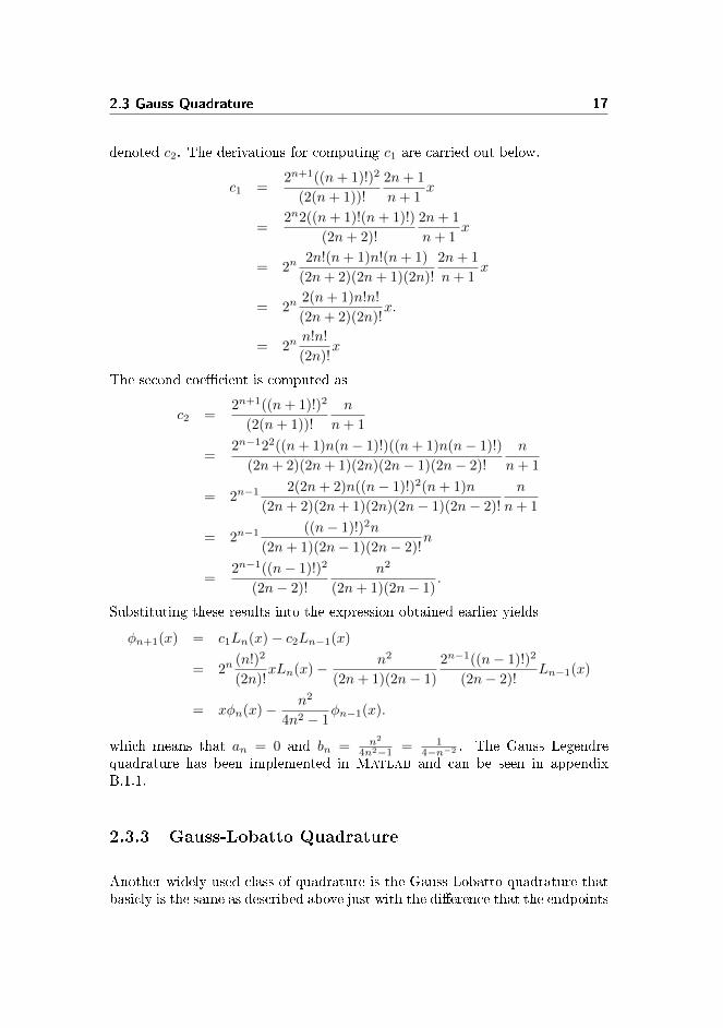
The derivations has been divided into two parts - one to compute the coecientin front of Ln(x) denoted c1 and one for the coecient in front of Ln−1(x)
2.3 Gauss Quadrature 17
denoted c2. The derivations for computing c1 are carried out below.
c1 =2n+1((n+ 1)!)2
(2(n+ 1))!
2n+ 1
n+ 1x
=2n2((n+ 1)!(n+ 1)!)
(2n+ 2)!
2n+ 1
n+ 1x
= 2n2n!(n+ 1)n!(n+ 1)
(2n+ 2)(2n+ 1)(2n)!
2n+ 1
n+ 1x
= 2n2(n+ 1)n!n!
(2n+ 2)(2n)!x.
= 2nn!n!
(2n)!x
The second coecient is computed as
c2 =2n+1((n+ 1)!)2
(2(n+ 1))!
n
n+ 1
=2n−122((n+ 1)n(n− 1)!)((n+ 1)n(n− 1)!)
(2n+ 2)(2n+ 1)(2n)(2n− 1)(2n− 2)!
n
n+ 1
= 2n−1 2(2n+ 2)n((n− 1)!)2(n+ 1)n
(2n+ 2)(2n+ 1)(2n)(2n− 1)(2n− 2)!
n
n+ 1
= 2n−1 ((n− 1)!)2n
(2n+ 1)(2n− 1)(2n− 2)!n
=2n−1((n− 1)!)2
(2n− 2)!
n2
(2n+ 1)(2n− 1).
Substituting these results into the expression obtained earlier yields
φn+1(x) = c1Ln(x)− c2Ln−1(x)
= 2n(n!)2
(2n)!xLn(x)− n2
(2n+ 1)(2n− 1)
2n−1((n− 1)!)2
(2n− 2)!Ln−1(x)
= xφn(x)− n2
4n2 − 1φn−1(x).
which means that an = 0 and bn = n2
4n2−1 = 14−n−2 . The Gauss Legendre
quadrature has been implemented in Matlab and can be seen in appendixB.1.1.
2.3.3 Gauss-Lobatto Quadrature
Another widely used class of quadrature is the Gauss-Lobatto quadrature thatbasicly is the same as described above just with the dierence that the endpoints

18 Mathematical background
are included in the quadrature nodes. This means that for example LegendreGauss-Lobatto quadrature with n quadrature points involves the zeros of a Leg-endre polynomial as well as the end points −1 and 1.The Gauss-Lobatto quadrature is generally not exact for as high orders of poly-nomials as the regular Gauss quadrature but it includes the end points whichcan be very useful in some cases, e.g. when solving boundary value problems,see [15]. Therefore the choice between Gauss quadrature and Gauss-Lobattoquadrature often depends on whether the boundary nodes plays a signicantrole or not for the solution.
2.4 Polynomial Interpolation
Polynomial interpolation is an approximation of a function f by use of polyno-mials, PM , which satises that f(xi) = PM (xi) for a given set of nodes xiNi=0.For the one dimensional case this yields
PM (xi) = aMxMi + · · ·+ a1xi + a0 = f(xi), i = 0, 1, . . . , N.
When using polynomial interpolation the Lagrange polynomials are a widelyused class of polynomials and the Lagrange polynomials, hi(x), are dened as
hi(x) =
M∏j=0,j 6=i
x− xjxi − xj
, i = 0, 1, . . . , N.
The Lagrange polynomials has a special property, namely
hj(xi) = δi,j =
1, i = j,
0, i 6= j,
where δi,j is the Kronecker delta function. The Lagrange polynomials are usedto establish a nodal representation on the form
f(x) =
N∑j=0
f(xj)hj(x),
and this form is called Lagrange form. Typically M = N since this yieldsa unique interpolating polynomial If(x) = QN (x). That QN (x) is unique isseen by assuming that another interpolating polynomial GN (x) exists such thatGN (xi) = f(xi) for i = 0, 1, . . . , N . The dierence between the two polynomialsis a new polynomial of order N , i.e. DN (x) = QN (x)−GN (x). This polynomialwill have N + 1 distinctive roots which implies that DN (x) is the zero polyno-mial and thereby that QN (x) is unique.

2.4 Polynomial Interpolation 19
Besides having a nodal representation in Lagrange form of the interpolatingpolynomial a modal representation can be used as well. In the nodal represen-tation introduced here it is the Lagrange polynomials hN (x) that are unknownbut in modal form the coecients are unknown and the polynomials are known -typically they are orthogonal polynomials like Legendre or Hermite polynomials.This means that the modal representation of f can be formulated as
fN (x) =
N∑j=0
fjΦj(x),
where the coecients typically are represented as
fj =1
γj
∫Dx
f(x)Φj(x)w(x)dx,
where Dx is the domain of x, w(x) is a weight chosen according to the polyno-mials Φj in order to secure orthogonality and γj is the normalization constantfor the polynomials.
2.4.1 Relationship between nodal and modal representa-
tions
Interpolating a function f in a discrete setting with polynomials is done by usinga modal or a nodal interpolating polynomial representation. By using Lagrangepolynomials h(x) as the nodal basis functions and appropriately chosen polyno-mials Φ(x) for the modal representation the following relationship between themodal and nodal representations can be established [7]
f(xi) =
N∑j=0
fjΦj(xi) =
N∑j=0
fjhj(xi), i = 0, . . . , N
where xi are the nodal interpolation points, which in this project typically aregenerated by use of a quadrature rule. The relationship between the modal andnodal coecients in the discrete interpolations can be expressed by use of theVandermonde matrix V which elements are computed as Vi,j = Φj(xi). Therelationship between the coecients can be expressed as
f = V f, (2.16)
where f and f are vectors containing the nodal and modal coecients, respec-
tively. Since the nodal and modal bases are related as fTh(x) = fT
Φ(x) the

20 Mathematical background
basis functions can also be related by use of the Vandermonde matrix. By useof (2.16) it is seen that the following holds
fTh(x) = (V f )Th(x) = fTVTh(x). (2.17)
This means that the bases can be related as
fTVT h(x) = f
TΦ(x)
mVTh(x) = Φ(x)
From this result it is clear that the Vandermonde matrix can transform thediscrete nodal basis functions into the discrete modal basis functions and viceversa.
2.5 Spectral methods
The theory introduced here about orthogonal polynomials serves as the basis forspectral methods. The orthogonal polynomials serves as a basis for polynomialexpansions on which the class of spectral methods is based on. The spectralmethods in general has spectral convergence which is one the main propertiesthat makes the methods attractive. The spectral methods for uncertainty quan-tication will be introduced in chapter 5.
2.6 Numerical solvers
In this section a numerical method for for solving PDE's in space will be outlined.Furthermore a method for solving PDE's in time is introduced.
2.6.1 Solver for dierential equations in space
When solving the dierential equations in space there are a lot of dierentmethods and approaches. In this section a spectral method for solving a non-periodic PDE is introduced.

2.6 Numerical solvers 21
2.6.1.1 Deterministic Collocation Method
The deterministic Collocation method is based on polynomial interpolation ofthe solution u which means that a set of interpolation points, xi, has to be chosen[7]. These points are typically known as collocation points and the Collocationmethod relies on a discrete nodal representation of the solution on the form
INu =
N∑i=0
unhn.
The collocation points used in this thesis will be chosen to be Gauss Lobattonodes. The deterministic Collocation method is based on a linear representa-tion of the solution and a linear operator L is introduced. This means that adierential equation on the form
d
dx
(adu
dx
)+ b
du
dx+ cu = f(x), x ∈ Dx, (2.18)
where Dx is the domain of x can be represented by a linear dierential operatordened as
L =d
dx
(ad
dx
)+ b
d
dx+ c. (2.19)
By introducing an interpolation derivative D as
Dv =d
dxINv (2.20)
a discrete expression for L denoted LN can be formulated for evaluation of anapproximation to the solution u in the interior collocation points. This meansthat
LN = D (AD) +BD + C, (2.21)
can be used to evaluate LN (INu(xi)) = f(xi) for i = 1, . . . , N − 1. Someadjustment are however necessary since the boundary conditions has not beenenforced yet.The boundary conditions can be enforced in dierent ways by modifying the es-tablished system of equations and this will be described in the implementationsection 8.2.1. For further information see [7].In order to use the deterministic Collocation method later on it has to be es-tablished how the spatial dierential matrix can be computed. This is outlinedin the following section.

22 Mathematical background
2.6.1.2 Construction of a spatial dierential matrix
By use of the Vandermonde matrix it is possible to construct a discrete operatorfor computing an approximation of the rst derivative in nodal space. The rstderivative in modal space can in discrete form be formulated as
d
dx
N∑j=0
fjΦj(x)
=
N∑j=0
fjd
dxΦj(x).
In matrix form this can be expressed as
df
dx= Vxf, Vx,ij =
dΦjdx
∣∣∣∣xi
.
In nodal space an approximation of the rst derivative in space can be expressedas
d
dx
N∑j=0
fjhj(x)
=
N∑j=0
fjd
dxhj(x).
In matrix form the nodal approximation can be formulated as
df
dx= Df, Di,j =
dhjdx
∣∣∣∣xi
,
where f is a vector containing the function evaluations. Now an expression forthe derivative matrix D can be derived.
df
dx= Df = D
(V f)
= Vx f,
where f is a vector containing the modal coecients and from this it is seen thatD = VxV−1. The matrices V and Vx can be expressed as
V =
Φ0(x1) Φ1(x1) · · · ΦN (x1)Φ0(x2) Φ1(x2) · · · ΦN (x2)
......
. . ....
Φ0(xN ) Φ1(xN ) · · · ΦN (xN )
and
Vx =
Φ0(x1)′ Φ1(x1)′ · · · ΦN (x1)′
Φ0(x2)′ Φ1(x2)′ · · · ΦN (x2)′
......
. . ....
Φ0(xN )′ Φ1(xN )′ · · · ΦN (xN )′
.The implementation of these matrices can be found in appendix B.

2.6 Numerical solvers 23
2.6.1.3 Legendre polynomials and the dierential matrix
In this thesis the Legendre polynomials will be used as basis polynomials in thedeterministic Collocation method. In practise the orthogonal basis polynomialsare often normalized [7] which means that the Vandermonde matrix can beexpressed as
V =
L0(x1) L1(x1) · · · LN (x1)
L0(x2) L1(x2) · · · LN (x2)...
.... . .
...
L0(xN ) L1(x2) · · · LN (xN )
, (2.22)
where Li(x) is the normalized i'th order Legendre polynomial. The Vander-monde matrix for the rst derivatives in space with regard to a Legendre basiscan be expressed as
Vx =
L0(x1)′ L1(x1)′ · · · LN (x1)′
L0(x2)′ L1(x2)′ · · · LN (x2)′
......
. . ....
L0(xN )′ L1(xN )′ · · · LN (xN )′
. (2.23)
This means that when an expression for the derivative of the Legendre poly-nomials has been established the spatial derivative matrix for a Legendre basiscan be computed. As a subclass of the Jacobi polynomials the derivatives of theLegendre polynomials can be derived from the expression for the derivatives ofthe Jacobi polynomial.In general the derivative of the Jacobi polynomials can be computed as
dk
dxkPα,βn (x) =
Γ(n+ α+ β + 1 + k)
2kΓ(n+ α+ β + 1)Pα+k,β+kn−k (x),
where Γ(a) = (a − 1)!. As mentioned earlier the orthonormal polynomials arefor computational reasons used instead of the standard polynomials and thenormalized Jacobi polynomials can be expressed as
Pα,βn (x) =Pα,βn (x)
γα,βn
. (2.24)
This means that the general expression for the derivative of the normalizedJacobi polynomials is
dk
dxkPα,βn (x) =
Γ(n+ α+ β + 1 + k)
2kΓ(n+ α+ β + 1)
γα+k,β+kn−k
γα,βn
Pα+k,β+kn−k (x).
24 Mathematical background
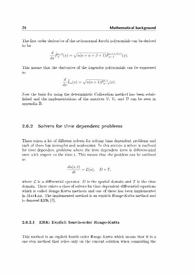
The rst order derivative of the orthonormal Jacobi polynomials can be derivedto be
d
dxPα,βn (x) =
√n(n+ α+ β + 1)Pα+1,β+1
n−1 (x).
This means that the derivative of the Legendre polynomials can be expressedas
d
dxLn(x) =
√n(n+ 1)P 1,1
n−1(x).
Now the basis for using the deterministic Collocation method has been estab-lished and the implementations of the matrices V, Vx and D can be seen inappendix B.
2.6.2 Solvers for time dependent problems
There exists a lot of dierent solvers for solving time dependent problems andeach of them has strengths and weaknesses. In this section a solver is outlinedfor time dependent problems where the time dependent term is dierentiatedonce with respect to the time t. This means that the problem can be outlinedas
du(x, t)
dt= L(u), D × T,
where L is a dierential operator, D is the spatial domain and T is the timedomain. There exists a class of solvers for time dependent dierential equationswhich is called Runge-Kutta methods and one of these has been implementedin MatLab. The implemented method is an explicit Runge-Kutta method andis denoted ERK [7].
2.6.2.1 ERK: Explicit fourth-order Runge-Kutta
This method is an explicit fourth-order Runge-Kutta which means that it is aone-step method that relies only on the current solution when computing the

2.6 Numerical solvers 25
next solution. The method can be outlined as
U = u(x, ti)
G = U
P = f(ti, U)
U = U + 12∆tP
G = P
P = f(ti + 12∆t, U)
U = U + 12∆t(P −G)
G = 16G
P = f(ti + 12∆t, U)− 1
2P
U = U + ∆tP
G = G− PP = f(ti + ∆t, U) + 2P
u(x, ti+1) = U + ∆t(G+ 16P )
where u(x, ti) denotes the current solution and u(x, ti+1) the solution in the nexttime step. The method has been implemented in Matlab in the le ERK.m andcan be seen in appendix B.

26 Mathematical background

Chapter 3
Basic concepts withinProbability Theory
This chapter will give a brief introduction to some basic concepts within prob-ability theory which are used in relation to Uncertainty Quantication. Theinterested reader can nd a more thorough description in [16] or [19].
3.1 Distributions and statistics
In order to cope with the stochastic problems investigated in this thesis somebasic denitions about distributions and statistics has to be introduced. Firstof all a random variable X has a (cumulative) distribution function, FX(x), anda (probability) density function. The distribution function, FX , is dened as acollection of probabilities that fulls
FX(x) = P (X ≤ x) = P (ω : X(ω) ≤ x). (3.1)
Due to the denition of the probability P it holds that 0 ≤ FX ≤ 1. The prob-ability density function, fX(x), is closely linked to the cumulative distribution

28 Basic concepts within Probability Theory
function through the relations
FX(a) =
∫ a
−∞fX(x)dx and fx(x) =
d
dxFX(x). (3.2)
The cumulative distribution function is as indicated by the name a cumulatedprobability in the sense that it computes the probability ofX being in an intervaland does not obtain any value in a single point. The density function on theother hand is intuitively a way of computing the probability in a point or in aninnitesimal interval.
3.1.1 Example: Gaussian distribution
A common and important class of distribution is the Gaussian distribution whichis also called the normal distribution and is denoted N (µ, σ2), where µ ∈ R isthe mean, σ2 > 0 is the variance and σ is called the standard deviation. Theprobability density function (PDF) can be formulated as
fX(x) =1√
2πσ2e−
(x−µ)2
2σ2 , x ∈ R. (3.3)
The distribution is often used with the parameters µ = 0 and σ2 = 1, i.e.N (0, 1), which is referred to as the standard normal distribution. The PDF forthe standard normal distribution is plotted in gure 3.1.

3.1 Distributions and statistics 29
−4 −3 −2 −1 0 1 2 3 4
0
0.1
0.2
0.3
0.4
x
f X(x
)
Figure 3.1: The PDF for the standard normal distribution.
3.1.2 Example: Uniform distribution
The uniform distribution is also an important class and its main characteristicis that all outcomes within the support of the distribution is equally probable.Furthermore the support is dened as an interval on the real line and charac-terized by IU = [a, b].The PDF of the uniform distribution is dened as
fX(x) =
1b−a x ∈ [a, b]
0 x /∈ [a, b]. (3.4)
The PDF for the uniform distribution with support IX = [0, 1] is plotted ingure 3.2

30 Basic concepts within Probability Theory
−1 0 1 2
0
0.2
0.4
0.6
0.8
1
x
f X(x
)
Figure 3.2: The PDF for the uniform distribution.
3.1.3 Multiple dimensions
In multiple dimensions it is useful to dene the joint density function and themarginal density function. The denitions given here will for simplicity be de-ned for two variables but it can be extended to any dimension. The denitionswill be based on [17].The joint density function is dened as a function f(x, y) that for −∞ < x, y <∞ fulls
f(x, y) ≥ 0 ∀x, y,∫∞−∞
∫∞−∞ f(x, y) dxdy = 1.
(3.5)
The multivariate cumulative distribution function can be dened as
F (a, b) =
∫ a
−∞
∫ b
−∞f(x, y) dxdy (3.6)
A new type of function can be introduced for the multivariate case namelythe marginal density function which is dened as fx(x) =
∫∞−∞ f(x, y) dy. The
function fx(x) has to full fx(x) ≥ 0 ∀x∫∞−∞ fx(x) dx = 1.
(3.7)

3.1 Distributions and statistics 31
The marginal density in y is dened equivalently and denoted fy(y).
3.1.4 Statistics
In this thesis there is mainly computed two statistics in the numerical investi-gations, namely the expectation and the variance. The expectation of a randomvariable X with density function Fx can be computed as
µX = E[X] =
∫IX
x dFX(x) =
∫IX
xfX d(x),
where IX is the domain of the variable and fX is the PDF. The variance of Xcan be computed as
σ2X = var(X) =
∫IX
(x− µX)2 dFX(x) =
∫IX
(x− µX)2 fXd(x).
Furthermore for m ∈ N the m'th moment of X can be computed as
E[Xm] =
∫IX
xm dFX(x) =
∫IX
xmfX d(x).
It is also possible to dene a moment generating function and an example ofthis can be seen in [19].
3.1.5 Inner product and statistics
In many cases it is possible to express the statistics in terms of inner prod-ucts. This of course requires the denition of an inner product and a properspace where this inner product is dened. The inner product was dened in adeterministic setting as (2.1) and in a stochastic setting it can be dened as
〈u, v〉dFX =
∫IX
u(X)v(X) dFX =
∫IX
u(X)v(X) fXd(x).
By comparing this denition with the denition of the statistics it is seen thatthe statistics can be represented by use of the inner product. This means forinstance that the expectation can be computed as
E[X] = 〈√X,√X〉dFX =
∫IX
x dFX(x) =
∫IX
xfX d(x).
The corresponding space is L2dFX
(IX) = f : IX → R |E[f2] < ∞ with the
norm dened by ‖f‖dFX =√E[f2].

32 Basic concepts within Probability Theory
3.2 Input parameterizations
The objective of this thesis is to study the eects of having uncertainty on theinput variables to a mathematical model. In practice this leads to some restric-tions on the input variables. To be usable in a computer they have to be niteand they should be independent, since most methods within the eld requirethis in practise. Two approaches for achieving this will be outlined here andthey are based on [16] and [19].
When the stochastic input is system parameters the input is already parametrized.The focus is therefore on ensuring the independence of the parameters. The pro-cedure can be outlined as in Algorithm 1.
Algorithm 1 Procedure for ensuring independence of stochastic system param-eters.
1: Let the system parameters be dened as Y = (Y1, . . . Yn) with n ≥ 1 andwith distribution function FY (y) = P (Y ≤ y) where y ∈ Rn.
2: Find a suitable transformation function T such that Y = T (Z) for Z =(Z1, . . . , Zd) ∈ Rd being a set of mutually independent random variables.
Similarly the approach can be outlined when the input parameters are stochasticprocesses which is seen in Algorithm 2.
Algorithm 2 Procedure for parameterization of random processes.
1: Let the stochastic process that models the stochastic inputs be dened as(Yk, k ∈ Dk) where k is an index belonging to the index set Dk. The indexk can belong to either a time or a space domain.
2: Find a suitable transformation function T such that Yk = T (Z) for Z =(Z1, . . . , Zd) with d ≥ 1 being a set of mutually independent random vari-ables.
Often the stochastic process is not nite dimensional which means some kind ofnite approximation has to be established. This introduces the problem withprecision contra eciency of the numerical solvers. An increasing number ofterms in the nite approximation usually leads to increasing precision but alsoleads to more computational work. For more information see [16] and [19].

Chapter 4
Generalized PolynomialChaos
The Generalized Polynomial Chaos (gPC) is outlined in this section. The gPCexpansions described in the following are based on smooth orthogonal polynomi-als such as Hermite polynomials or Legendre polynomials. In fact the originalpolynomial chaos was based on Hermite polynomials and proved to be quiteeective, when the stochastic parameters are Gaussian distributed but gener-ally it is slow for non-Gaussian distributed variables. Therefore the gPC wasintroduced where the orthogonal basis polynomials are chosen according to thedistribution of the stochastic parameters.The gPC is a way of representing a stochastic process X(ω) parametrically. Thisis done by using an expansion with orthogonal polynomials such that a randomeld X(ω) can be represented by
X(ω) =
∞∑j=0
cjΦj(ω),
where Φ represent the given basis polynomial and ω the random variable(s).The polynomials are chosen such that the weights that ensures the orthogonalproperty 〈Φi,Φj〉 =
∫D
Φi(x)Φj(x)w(x)dx = 〈Φ2i 〉δi,j resembles the probabil-
ity distribution function of the random variables. If a random variable, ω, isstandard normal distributed it means that the probability density function is
34 Generalized Polynomial Chaos
1√2πe−
12σ
2
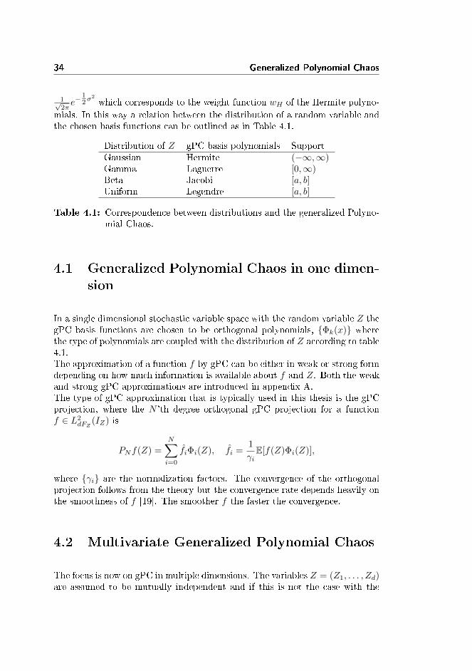
which corresponds to the weight function wH of the Hermite polyno-
mials. In this way a relation between the distribution of a random variable andthe chosen basis functions can be outlined as in Table 4.1.
Distribution of Z gPC basis polynomials SupportGaussian Hermite (−∞,∞)Gamma Laguerre [0,∞)Beta Jacobi [a, b]Uniform Legendre [a, b]
Table 4.1: Correspondence between distributions and the generalized Polyno-mial Chaos.
4.1 Generalized Polynomial Chaos in one dimen-
sion
In a single dimensional stochastic variable space with the random variable Z thegPC basis functions are chosen to be orthogonal polynomials, Φk(x) wherethe type of polynomials are coupled with the distribution of Z according to table4.1.The approximation of a function f by gPC can be either in weak or strong formdepending on how much information is available about f and Z. Both the weakand strong gPC approximations are introduced in appendix A.The type of gPC approximation that is typically used in this thesis is the gPCprojection, where the N 'th degree orthogonal gPC projection for a functionf ∈ L2
dFZ(IZ) is
PNf(Z) =
N∑i=0
fiΦi(Z), fi =1
γiE[f(Z)Φi(Z)],
where γi are the normalization factors. The convergence of the orthogonalprojection follows from the theory but the convergence rate depends heavily onthe smoothness of f [19]. The smoother f the faster the convergence.
4.2 Multivariate Generalized Polynomial Chaos
The focus is now on gPC in multiple dimensions. The variables Z = (Z1, . . . , Zd)are assumed to be mutually independent and if this is not the case with the
4.2 Multivariate Generalized Polynomial Chaos 35
stochastic variables in the original problem a parametrization can be conductedin order to achieve the independence of the variables.The variables Zi have support IZi and marginal distribution PZi(zi) = P (Zi <zi) and since the variables are independent it holds that
FZ(z1, . . . , zd) = P (Z1 ≤ z1, . . . , Zd ≤ zd) =
d∏i=1
FZi(Zi),
and IZ = IZ1× · · · × IZd .
For the variable Zi a corresponding set of univariate gPC basis functions areintroduced, i.e. φk(Zi)Nk=0 ∈ PN (Zi), which are polynomials in Zi of degreeup to N .
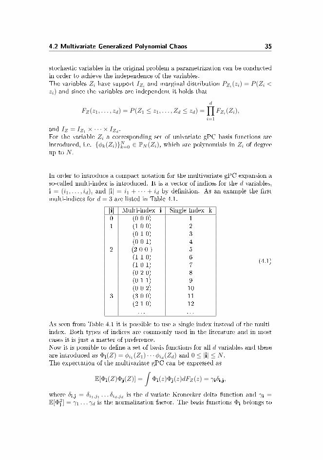
In order to introduce a compact notation for the multivariate gPC expansion aso-called multi-index is introduced. It is a vector of indices for the d variables,i = (i1, . . . , id), and |i| = i1 + · · · + id by denition. As an example the rstmulti-indices for d = 3 are listed in Table 4.1.
|i| Multi-index i Single Index k0 (0 0 0) 11 (1 0 0) 2
(0 1 0) 3(0 0 1) 4
2 (2 0 0 ) 5(1 1 0) 6(1 0 1) 7(0 2 0) 8(0 1 1) 9(0 0 2) 10
3 (3 0 0) 11(2 1 0) 12. . . . . .
(4.1)
As seen from Table 4.1 it is possible to use a single index instead of the multi-index. Both types of indices are commonly used in the literature and in mostcases it is just a matter of preference.Now it is possible to dene a set of basis functions for all d variables and theseare introduced as Φi(Z) = φi1(Z1) · · ·φid(Zd) and 0 ≤ |i| ≤ N .The expectation of the multivariate gPC can be expressed as
E[Φi(Z)Φj(Z)] =
∫Φi(z)Φj(z)dFZ(z) = γiδi,j,
where δi,j = δi1,j1 . . . δid,jd is the d-variate Kronecker delta function and γi =E[Φ2
i ] = γ1 . . . γd is the normalization factor. The basis functions Φi belongs to

36 Generalized Polynomial Chaos
the polynomial space
PdN (Z) = p : IZ → R| p(Z) =∑|i|≤N
ciΦi(Z),
which has the dimension dimPdN =
(N + dN
). Otherwise the polynomials
Φi(Z) can be dened to be of degree up to N in each dimension which implies apolynomial space, PdN , of dimension dim PdN = Nd. This choice of space usuallyresults in too many basis functions to be evaluated in practise for large dimen-sions.
As in the univariate case a multivariate gPC projection can be dened as
PNf =∑|i|≤N
fiΦi(Z),
where the coecients can be computed as
fi =1
γiE[fΦi] =
1
γi
∫f(z)Φi(z)dFZ(z), ∀|i| ≤ N.
The d-variate gPC projection is conducted in the space L2dFZ
which is denedas (2.2).
4.3 Statistics for gPC expansions
The gPC expansions can be used not only to approximate a function f but alsoto estimate the statistics of f . If u(x, t, Z) is a random process with x ∈ Dx,t ∈ T and Z ∈ Rd then the N 'th order gPC expansion can be expressed as
uN (x, t, Z) =∑|i|≤N
ui(x, t)Φi(Z) ∈ PdN ,
for any xed x ∈ Dx and t ∈ T . The orthogonality of the basis functionsenables the following computations of the statistics. For instance the meancan be approximated as E[u(x, t, Z)] ≈ E[uN (x, t, Z)] and the computation of
4.3 Statistics for gPC expansions 37
E[uN (x, t, Z)] yields
E[uN (x, t, Z)] =
∫ ∑|i|≤N
ui(x, t)Φi(z)
dFZ(z)
=
∫ ∑|i|≤N
ui(x, t)Φi(z)
Φ0(z)dFZ(z)
= u0(x, t).
The orthogonality of the basis functions has been utilized as well as the fact thezero-order polynomial Φ0(Z) is dened to be ones which explains how it couldbe introduced in the second equality. The variance can be computed as
var(u(x, t, Z)) = E[(u(x, t, Z)− µu(x, t))2].
By using uN the variance can be approximated by
E[(uN (x, t, Z)− µuN (x, t))2] =
∫ ∑|i|≤N
ui(x, t)Φi(z)− u0(x, t)
2
dFZ(z)
=
∫ ∑0<|i|≤N
ui(x, t)Φi(z)
2
dFZ(z)
=∑
0<|i|≤N
u2i (x, t)γi.
where the orthogonality ensures the validity of the second to last equality signsince ∫
(ui(x, t)Φi(z)) (uj(x, t)Φj(z)) dFZ(z) = 0 for i 6= j.
Other statistics can be approximated as well by applying their denitions to thegPC approximation uN [19].

38 Generalized Polynomial Chaos

Chapter 5
Stochastic SpectralMethods
Uncertainty Quantication (UQ) will in this project be with regard to solvingPartial Dierential Equations (PDEs). The PDEs in this thesis can in general fora time domain T and spatial domain D ⊂ R` with ` = 1, 2, 3, . . . be formulatedas
ut(x, t, ω) = L(u), D × T × Ω
B(u) = 0, , ∂D × T × Ω
u = u0, ∂D × [t = 0]× Ω,
where ω ∈ Ω are the random inputs of the system in a probability space(ω,F , P ), L is a dierential operator, B is the boundary condition (BC) op-erator and u0 is the initial condition (IC).In many cases it is required to restate the random variables ω such that aparametrization, Z = (Z1, . . . , Zd) ∈ Rd with d ≥ 1, consisting of independentrandom variables is used instead. This means that the PDE system is on theform
ut(x, t, Z) = L(u), D × T × Rd
B(u) = 0, ∂D × T × Rd (5.1)
u = u0, ∂D × [t = 0]× Rd,
40 Stochastic Spectral Methods
This general formulation will be used in the following when introducing thetechniques for UQ.
5.1 Non-intrusive methods
The non-intrusive methods are generally speaking a class of methods which re-lies on realizations of the stochastic system - i.e. deterministic solutions of theunderlying non-stochastic system. This is an interesting feature of the non-intrusive methods for stochastic systems, since well-known solvers can be usedwithout any particular modications. Another interesting part is when the de-terministic solutions are decoupled the solutions can be computed in parallel.A drawback with the non-intrusive methods is the computational eort thatgrows with the number of deterministic solutions to be computed. This draw-back will be further described later and is an important topic in UQ.
5.1.1 Monte Carlo Sampling
The Monte Carlo Sampling (MCS) is based on constructing a system of inde-pendent and identical distributed (i.i.d.) variables Z. Then a system like (5.1)is solved as a deterministic system for M dierent realizations of Z and therebyobtaining M solutions of the type u(i)(x, t) = u(x, t, Zi), where Zi refers to thei'th realization of Z.When the M solutions have been computed the solution statistics can be esti-mated. For example the mean of the solution can be estimated according to theCentral Limit Theorem (CLT) as
u =1
M
M∑i=1
ui.
This is as mentioned only an estimation of the true mean, u ≈ E(u) = µu, andan error estimate of MCS follows from the CLT [19].Since the M solutions u(x, t, Zi) are i.i.d. it means that for M → ∞ the
distribution of u converges towards a Gaussian distributionN (µu,σ2u
M ), where µuand σu are the exact mean and standard deviation of the solution, respectively.This means that the standard deviation of the Gaussian distribution is M−
12σu
and from this the convergence rate is established as O(M−12 ) [19].
It is important to note that only two requirements are to be met in order touse MCS. Namely that the system is on the right form and that a solver forthe deterministic system is at hand. When these requirements are fullled a

5.1 Non-intrusive methods 41
convergence rate of O(M−12 ) can be obtained independently of the dimension
of the random space, which is quite unique. It is however worth noting that theconvergence rate is rather slow and if the deterministic solver is time consumingthen it will take an immense amount of time to obtain a decent accuracy on theestimates of the statistics.It should also be mentioned that there exists several methods which are basedon the Monte Carlo method but has e.g. better eciency. These methods aregenerally known as Quasi-Monte Carlo methods but it lies outside the scope ofthis thesis to investigate these methods.
5.1.2 Stochastic Collocation Method
The stochastic collocation method (SCM) is a stochastic expansion methodthat in general relies on expansion through Lagrange interpolation polynomials.The overall idea is to choose a set of collocation points ZM = ZjMj=1 in the
random space. Then (5.1) is enforced in each of the nodes Zj which means thatthe following system is solved for j = 1, . . . ,M
ut(x, t, Zj) = L(u), D × T × Rd
B(u) = 0, , ∂D × T × Rd
u = u0, ∂D × [t = 0]× Rd.
This system is deterministic for each j and hence the SCM involves solving Mdeterministic systems. This is a very broad denition of the SCM and it wouldinclude the Monte Carlo sampling. Usually when using the SCM a clever choiceof collocation points is made - e.g. choosing the points by a quadrature rule andexploit the belonging quadrature weights when computing the statistics.The solution of the PDE (5.1) can be representated by use of Lagrange inter-polating functions which have been described earlier. Hence the solution u isrepresented by an interpolation
u(Z) ≡ I(u) =
M∑j=1
u(Zj)hj(Z), (5.2)
where hj are the Lagrange polynomials and u(Zj) = u(x, t, Zj). It is importantto remember that the Lagrange polynomials are dened in a appropriate inter-polation space VI and that hi(Z
j) = δij for i, j ∈ [1, . . . ,M ]. This means thatthe interpolation u(Z) is equal to the exact solution in each of theM collocationpoints.FromM deterministic solutions in the collocation points the statistics of the in-terpolation can be computed and thereby represent the statistics of the stochas-

42 Stochastic Spectral Methods
tic solution to (5.1). The mean of the interpolation u can for instance be com-puted as
E[u] =
M∑j=1
u(Zj)
∫Γ
hj(z)ρ(z)dz, (5.3)
where Γ is the random space in which Z is dened and ρ(z) is a distributionspecic weight - namely the probability density function of the distribution ofZ. The evaluation of the expectation can be non-trivial and knowledge of theLagrange polynomials is needed. This can be obtained by use of an invertedVandermonde-type matrix but it often requires quite a lot of work [20].Another approach is to use a quadrature rule to evaluate the integral whichleads to
E[u] =
M∑j=1
u(Zj)
M∑k=1
hj(zk)ρ(zk)wk, (5.4)
where zk are the quadrature points and wk are the quadrature weights. Theapproximation of the integral in (5.3) by quadrature is exact since the Lagrangepolynomials are of order M and the quadrature is exact for polynomials of thisorder.The attained expression for the mean of the interpolation can be further sim-plied by choosing the collocation points smartly. The quadrature nodes andweights are chosen so they represent the distribution of the random parameters.This means that the quadrature points could be chosen as collocation points,i.e. zj = Zj . Hence the characteristic of the Lagrange polynomials, hi(Z
j) = δijfor i, j ∈ [1, . . . ,M ], can be exploited once again and (5.4) reduces to
E[u] =
M∑j=1
u(Zj)ρ(Zj)wj .
In the same way the variance of the interpolation can be computed as
var[u] = E[(u− E[u])2]
=
∫Γ
(u− E[u])2ρ(z)dz
=
∫Γ
M∑j=1
u(Zj)hj(z)− E[u]
2
ρ(z)dz
=
M∑k=1
M∑j=1
u(Zj)hj(zk)− E[u]
2
ρ(zk)wk.
where the integral of the expectation is evaluated by use of the appropriatequadrature rules. Again the quadrature points and collocation points could be
5.2 Intrusive methods 43
the same points which leads to
var[u] =
M∑k=1
M∑j=1
u(Zj)δij − E[u]
2
ρ(Zk)wk.
=
M∑k=1
(u(Zk)− E[u]
)2ρ(Zk)wk.
In the same way other statistics could be computed as well if needed. Theapproach outlined here is an interpolation approach but there is another commonapproach within the stochastic Collocation methods which is referred to as apseudo-spectral approach which uses discrete projection. This approach willhowever not be pursued further but more information can be found in e.g. [19].
5.2 Intrusive methods
Unlike the non-intrusive methods the intrusive methods rely on modifying theinitial problem and in this project the focus will be on the intrusive polynomialchaos (PC) methods that relies on a weighted residual formalism.These methods leads to spectral convergence but on the contrary to the non-intrusive methods implies extra analytical and numerical work. The modi-cation of the stochastic system to be solved can be very troublesome and theresulting stochastic system often requires solvers that are dierent from theusual deterministic solvers [16]. Hence it is a trade-o between the extra ana-lytical and numerical work and the much appreciated convergence.When using stochastic Galerkin-like methods many of the properties from thedeterministic Galerkin method is inherited - e.g. that the representation is op-timal in the mean-square error [16].
5.2.1 Stochastic Galerkin method
The stochastic gPC Galerkin method (SGM) is a intrusive spectral method thatrelies on spectral approximations using generalized Polynomial Chaos (gPC).The idea of the SGM method is to dene a solution in the space of polyno-mials such that the residue of the system (5.1) is orthogonal to the space ofpolynomials. The general approach is outlined in algorithm 3.

44 Stochastic Spectral Methods
Algorithm 3 Outline for the Stochastic Galerkin Method.
1: Identify the source of uncertainty and compute a set of independent randomvariables with an appropriate PDF to represent this.
2: Construct a generalized Polynomial Chaos basis and use this to construct agPC expansion to represent the system.
3: Modify the governing system by substituting with the gPC expansion.4: Apply the Galerkin procedure to obtain a set of coupled deterministic equa-
tions instead of stochastic equations.5: Use appropriate numerical methods to solve the system of equations.6: Post-processing - compute the needed statistics from the obtained solution.
For further information about this general outline see [12]. In the general system(5.1) the uncertainty has been identied and is described by the independentparameters Z = (Z1, . . . , Zd) ∈ Rd where d ≥ 1.The gPC basis is chosen so it matches the distribution of the random parametersZ and this correspondence is outlined for the most common distributions inTable 4.1. The gPC basis is denoted Φk(Z)Nk=0 and belongs to the space PdNthat consists of all the polynomials in Z of degree up to N . As described earlierthe gPC basis consists of orthogonal polynomials in the random space whichmeans that E[ΦkΦj ] = δkjγk.The approximation by a gPC expansion of the solution to (5.1) can be describedas
u(x, t, Z) ≈ uN (x, t, Z) =
N∑|i|=0
ui(x, t)Φi(Z), (5.5)
where i is the multi-index described earlier and
ui(x, t) =1
γiE[u(x, t, Z)Φi].
This means that the number of terms in (5.5) is P + 1 = (N+d)!(d)!(N)! . By using the
single index described earlier and by dening ΦpP+1p=0 as the collection of basis
polynomials the gPC expansion of the solution can be expressed as in [12] by
uN (x, t, Z) =
P+1∑p=0
up(x, t)Φp(Z), (5.6)
where
up(x, t) =1
γpE[u(x, t, Z)Φp].
Now the Galerkin procedure is performed by a Galerkin projection of (5.5) or(5.6) onto the space spanned by the polynomial basis. This is done by suc-cessively applying the inner product between the given equation and each of

5.2 Intrusive methods 45
the basis functions, i.e. evaluating the expectation for each index. By use ofmulti-index k where k ≤ N this leads to a new formulation of the system (5.1),namely
E[∂
∂tuN (x, t, Z)Φk(Z)] = E[L(uN )Φk(Z)], D × T × Rd
E[B(uN )Φk(Z)] = 0, ∂D × T × Rd (5.7)
uk = v0,k, ∂D × [t = 0]× Rd,
where the gPC projection coecients v0,k of the initial condition more explicitly
can be written as v0,k = E[u0Φk(Z)]γk
. By evaluation of the expectations thesystem is reduced to a set of deterministic equations that usually are coupled.This means that the system is independent of the random parameters Z.It follows from the gPC theory how to compute the statistics of the stochasticsolution by computing the solution to the deterministic system (5.8). The meanand variance can for instance be computed as
µu(x,t) ≈ E[uN (x, t, Z)] = u0(x, t), σ2u ≈ σ2
u =
N∑|i|=1
γiu2i (x, t).
For further information see [19] and [12].

46 Stochastic Spectral Methods
Chapter 6
Test problems
In this section two test problems are introduced. The rst is a simple OrdinaryDierential Equation (ODE) known as the (stochastic) Test Equation which willserve as a toy problem for testing convergence and eciency of the methods.The second model problem is the partial dierential equation (PDE) denotedBurgers' Equation which is more complex and involves a non-linear term. In thischapter the book [18] is used as a general reference when evaluating integrals.
6.1 Test Equation
In this section the ODE known as the Test Equation is introduced. The ODElooks like this with deterministic parameters
d
dtu(t) = −λu(t), u(0) = b.
With stochastic parameters the ODE looks like this
d
dtu(t, ω) = −α(ω)u(t, ω), u(0, ω) = β(ω). (6.1)
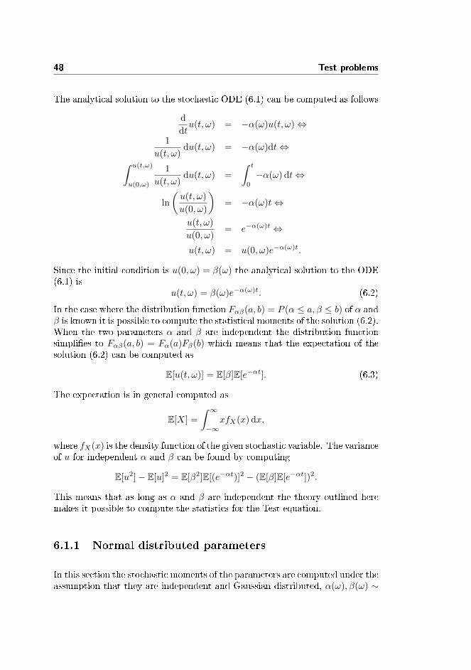
48 Test problems
The analytical solution to the stochastic ODE (6.1) can be computed as follows
d
dtu(t, ω) = −α(ω)u(t, ω)⇔
1
u(t, ω)du(t, ω) = −α(ω)dt⇔∫ u(t,ω)
u(0,ω)
1
u(t, ω)du(t, ω) =
∫ t
0
−α(ω) dt⇔
ln
(u(t, ω)
u(0, ω)
)= −α(ω)t⇔
u(t, ω)
u(0, ω)= e−α(ω)t ⇔
u(t, ω) = u(0, ω)e−α(ω)t.
Since the initial condition is u(0, ω) = β(ω) the analytical solution to the ODE(6.1) is
u(t, ω) = β(ω)e−α(ω)t. (6.2)
In the case where the distribution function Fαβ(a, b) = P (α ≤ a, β ≤ b) of α andβ is known it is possible to compute the statistical moments of the solution (6.2).When the two parameters α and β are independent the distribution functionsimplies to Fαβ(a, b) = Fα(a)Fβ(b) which means that the expectation of thesolution (6.2) can be computed as
E[u(t, ω)] = E[β]E[e−αt]. (6.3)
The expectation is in general computed as
E[X] =
∫ ∞−∞
xfX(x) dx,
where fX(x) is the density function of the given stochastic variable. The varianceof u for independent α and β can be found by computing
E[u2]− E[u]2 = E[β2]E[(e−αt)]2 − (E[β]E[e−αt])2.
This means that as long as α and β are independent the theory outlined heremakes it possible to compute the statistics for the Test equation.
6.1.1 Normal distributed parameters
In this section the stochastic moments of the parameters are computed under theassumption that they are independent and Gaussian distributed, α(ω), β(ω) ∼

6.1 Test Equation 49
N (µ, σ2). The density function for a Gaussian distribution is given as
fX(x) =1√
2πσ2exp
[− (x− µ)2
2σ2
]. (6.4)
The expectation of e−αt can therefore be computed as follows
E[e−αt
]=
∫ ∞−∞
(e−xt)
(1√
2πσ2e−
12σ2
(x−µ)2)
dx
=
∫ ∞−∞
1√2πσ2
e−1
2σ2(x2+µ2−2xµ)−xtdx
=
∫ ∞−∞
1√2πσ2
e−1
2σ2(x2+µ2−2xµ+2σ2xt)dx
=
∫ ∞−∞
1√2πσ2
e−1
2σ2(x2+µ2−2(µ−σ2t)x)dx. (6.5)
Now the variable µ = µ−σ2t is introduced. By using this variable it is possibleto rewrite (6.5) in a convenient way when using that by the denition of µ thefollowing holds.
(x− µ)2 = x2 + µ2 − 2xµ
= x2 + (µ2 + (σ2t)2 − 2µσ2t)− 2(µ− σ2t)x
= x2 + µ2 − 2(µ− σ2t)x+ σ4t2 − 2µσ2t. (6.6)
It is noticed that the exponent of the exponential function equals (6.6) exceptfor σ4t2 − 2µσ2t. Hence (6.5) can be rewritten as
E[u] =
∫ ∞−∞
1√2πσ2
e−1
2σ2((x−µ)2−(σ4t2−2µσ2t))dx
= e−1
2σ2(−σ4t2+2µσ2t))
∫ ∞−∞
1√2πσ2
e−1
2σ2((x−µ)2)dx
= e12σ
2t2−µt. (6.7)
In the second equation it is recognized that the expression inside the integralis a density function for a normal distribution N (µ, σ2) and the integral over adensity function equals one. The variance of e−αt can be computed as
var(e−αt) = E[(e−αt)2]− (E[e−αt])2,
and from (6.7) it follows that (E[e−αt])2 = eσ2t2−2µt. To compute E[(e−αt)2] =
E[e−2xt] the same procedure as used to compute the expectation will lead to
E[u2] = e2σ2t2−2µt. Hence the mean and variance are given as
var(e−αt) = E[e−αt
]= e
12σ
2t2−µt. (6.8)

50 Test problems
and
E[(e−αt)2]− (E[e−αt])2 = e2σ2t2−2µt − eσ2t2−2µt. (6.9)
The statistical moments of a Gaussian distributed β-parameter can also becomputed. The mean of β is
E[β] =
∫ ∞−∞
x
(1√
2πσ2e−
(x−µ)2
2σ2
)dx
=1√
2πσ2
∫ ∞−∞
xe−1
2σ2(x−µ)2 dx
=1√
2πσ2µ
√π1
2σ2
= µ.
The integral in the second equation has been evaluated according to [18] andthe result is in good correspondence with the theory - the mean of a normaldistributed parameter should be equal to the distribution mean. To computethe variance of β the following from [18] is used
∫ ∞−∞
e−ax2
dx =
√π
a. (6.10)
When dierentiating both sides of (6.10) with regard to a the following usefulresult is achieved
d
da
∫ ∞−∞
e−ax2
dx =
∫ ∞−∞−x2e−ax
2
dx =d
da
√π
a= − 1
2a
√π
a.
This means that ∫ ∞−∞
x2e−ax2
dx =1
2a
√π
a. (6.11)
In order to compute the variance of β the term E[β2]has to be computed which
can expressed as
E[β2]
=
∫ ∞−∞
x2
(1√
2πσ2e−
(x−µ)2
2σ2
)dx.
Now a new variable is introduced, namely x = x − µ which implies x = x + µ.This also means that
x2 = µ2 + x2 + 2µx. (6.12)

6.1 Test Equation 51
Furthermore a = 12σ2 is introduced which means that E
[β2]can be expressed
as
E[β2]
=
∫ ∞−∞
x2
(1√
2πσ2e−
(x−µ)2
2σ2
)dx
=
∫ ∞−∞
(µ2 + x2 + 2µx
) 1√2πσ2
e−ax2
dx
=µ2∫∞−∞e
−ax2
dx+∫∞−∞ x2e−ax
2
dx+ 2µ∫∞−∞ xe−ax
2
dx√
2πσ2.(6.13)
The last integral in (6.13) can be evaluated to be zero by substituting withx = x− µ which gives∫ ∞
−∞(x− µ)e−a(x−µ)2 dx =
∫ ∞−∞
xe−a(x−µ)2 dx− µ∫ ∞−∞
e−a(x−µ)2 dx
= µ
√π
a− µ
√π
a= 0.
The rst of the two obtained integrals is the same as appeared in the compu-tation of the mean and is known to be equal to µ
√2πσ2 which is the same as
µ√
πa . The last integral is the same as in (6.10) and therefore evaluates to
√πa .
Now it is possible to evaluate (6.13) since he rst integral in (6.13) is recognizedto be of the type (6.10), the second is the same as in (6.11) and the last integralevaluates to zero. Hence (6.13) becomes
E[β2]
=1√
2πσ2
(1
2a
√π
a+ µ2
√π
a+ 2µ · 0
)=
1√2πσ2
(2σ2
2
√π2σ2 + µ2
√2πσ2
)= σ2 + µ2,
where the second equation results from substituting with a = 12σ2 . This means
that variance of β is var(β) = (σ2 + µ2) − µ2. The mean and variance ofβ ∼ N (µβ , σ
2β) is therefore
E[β] = µ,
var(β) = σ2.
6.1.2 Uniform distributed parameters
The parameters can also be uniform distributed and in this section the statisticalmoments for this case are computed. The density function for the uniform

52 Test problems
distribution is
fX(x) =
1b−a x ∈ (a, b),
0 otherwise.(6.14)
First the statistics of e−αt are computed and the expectation can be computedas
E[e−αt
]=
∫ b
a
e−xt1
b− adx
=1
b− a
(1
−t
)[e−xt
]ba
= −e−bt − e−at
t(b− a). (6.15)
Now E[(e−αt)
2]is computed as
E[(e−αt
)2]=
∫ b
a
e−2xt 1
b− adx
=1
b− a
(1
−2t
)[e−2xt
]ba
= −e−2bt − e−2at
2t(b− a). (6.16)
This means that the variance is
E[(e−αt
)2]− E[e−αt
]2= −e
−2bt − e−2at
2t(b− a)−(−e−bt − e−at
t(b− a)
)2
= −e−2bt − e−2at
2t(b− a)−(e−bt − e−at
)2t2(b− a)2
. (6.17)
The expectation and variance of β when β is uniformly distributed can also becomputed and is
E[β] =
∫ b
a
x1
b− adx =
1
b− a
[1
2x2
]ba
=1
2
b2 − a2
b− a=
1
2
(b+ a)(b− a)
b− a
=1
2(b+ a). (6.18)
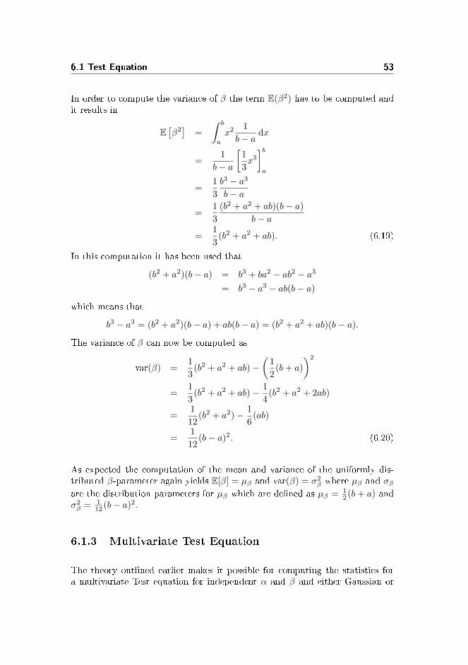
6.1 Test Equation 53
In order to compute the variance of β the term E(β2) has to be computed andit results in
E[β2]
=
∫ b
a
x2 1
b− adx
=1
b− a
[1
3x3
]ba
=1
3
b3 − a3
b− a
=1
3
(b2 + a2 + ab)(b− a)
b− a
=1
3(b2 + a2 + ab). (6.19)
In this computation it has been used that
(b2 + a2)(b− a) = b3 + ba2 − ab2 − a3
= b3 − a3 − ab(b− a)
which means that
b3 − a3 = (b2 + a2)(b− a) + ab(b− a) = (b2 + a2 + ab)(b− a).
The variance of β can now be computed as
var(β) =1
3(b2 + a2 + ab)−
(1
2(b+ a)
)2
=1
3(b2 + a2 + ab)− 1
4(b2 + a2 + 2ab)
=1
12(b2 + a2)− 1
6(ab)
=1
12(b− a)2. (6.20)
As expected the computation of the mean and variance of the uniformly dis-tributed β-parameter again yields E[β] = µβ and var(β) = σ2
β where µβ and σβare the distribution parameters for µβ which are dened as µβ = 1
2 (b + a) andσ2β = 1
12 (b− a)2.
6.1.3 Multivariate Test Equation
The theory outlined earlier makes it possible for computing the statistics fora multivariate Test equation for independent α and β and either Gaussian or

54 Test problems
uniform distributed. The procedure is the same for all the combinations of dis-tributions of the two variables and therefore only two cases will be introduced.
6.1.3.1 Gaussian distributed α and β
When α and β are independent and Gaussian distributed the mean can be com-puted by use of the terms computed in chapter 6.1.1. The mean can thereforebe computed as
E[u] = E[β]E[e−αt]
= µβe12σ
2t2−µt.
The terms for computing the variance can also be reused to computed the vari-ance of the multivariate ODE. The terms are
E[(e−αt)2] = e2σ2t2−2µt
(E[e−αt])2 = eσ2t2−2µt
E[β2] = σ2 + µ2β
E[β]2 = µ2β .
This means that the variance can be computed as
var(u) = (σ2 + µ2β)e2σ2t2−2µt − µ2
βeσ2t2−2µt. (6.21)
6.1.3.2 Gaussian distributed α and uniformly distributed β
Now it is assumed that α is Gaussian distributed and β is uniformly distributedand that they are mutually independent. The mean and variance can be com-puted in the same manner as when both of them where Gaussian distributed.The mean is computed as
E[u] = E[β]E[e−αt]
= µβe12σ
2t2−µt.

6.2 Burgers' Equation 55
Again the terms used for computing the variance has already been computed tobe
E[(e−αt)2] = e2σ2t2−2µt
(E[e−αt])2 = eσ2t2−2µt
E[β2] =1
3(b2 + a2 + ab)
E[β]2 = (1
2(b+ a))2 = µ2
β .
This means that the variance can be computed as
var(u) =1
3(b2 + a2 + ab)e2σ2t2−2µt − µ2
βeσ2t2−2µt.
In the same way other combinations of the independently distributed variablesα and β could be computed.
6.2 Burgers' Equation
The viscous Burgers' equation is a classic example of a non-linear PDE and itis dened as
ut + uux = νuxx, x ∈ [−1, 1] ,
u(−1) = 1,
u(1) = −1,
(6.22)
where ν is the viscosity and u is the solution eld. Burgers' equation is aninteresting PDE to study since it contains both time and space derivatives, anon-linear term and has several interesting properties. One property that isinteresting from an UQ point of view is that the PDE is supersensitive towardsdisturbances in the boundary condition [19]. This feature will be investigatedin the numerical experiments later on.The solution to Burgers' equation is plotted in gure 6.1 for t = 0 and it is seenthat it is more or less constant 1 until it reaches a transition layer and shifts tobe close to −1.

56 Test problems
−1 −0.5 0 0.5 1
−1
−0.5
0
0.5
1
x
u
Figure 6.1: The deterministic solution for Burgers' equation for t = 0.
The focus of this thesis is on Uncertainty Quantication (UQ) and thereforea stochastic Burgers' equation is introduced. The stochastic Burgers' equationused in the 1D test cases is formulated as
ut + uux = νuxx, x ∈ [−1, 1] ,
u(−1) = 1 + δ(Z),
u(1) = −1,
(6.23)
where δ(Z) is a random perturbation of the boundary. This means that theleft boundary condition has been perturbed by additive noise. The eects ofhaving a stochastic ν and right boundary have also been investigated but theseexperiments are conducted later on.The eects of a stochastic boundary condition is clear when the solution isplotted for the deterministic system with the left boundary condition u(−1) = 1and the system with u(−1) = 1.01.

6.2 Burgers' Equation 57
−1 −0.5 0 0.5 1
−1
−0.5
0
0.5
1
x
u
u1(x)
u1.01(x)
Figure 6.2: The deterministic solution for Burgers' equation with boundaryconditions u(−1) = 1 and u(−1) = 1.01.
Figure 6.2 illustrates that the solution is very dependent on how the boundaryconditions are formulated since the transition layer moves quite a lot even thoughthe left BC is perturbed by only 1 %.

58 Test problems
Chapter 7
Test of UQ methods on theTest Equation
In this chapter the three UQ methods will be used to solve the Test Equationand test their qualities and drawbacks. The implementations of the methodswill be outlined here and all the code can be found in appendix B.
7.1 Monte Carlo Sampling
In this section the results from the Monte Carlo Sampling will be examined.The approach can be outlined as
Algorithm 4 Pseudocode for Monte Carlo Sampling applied to the Test Equa-tion
1: Compute N realizations of the stochastic variable α.2: Solve the deterministic system to obtain the N deterministic solutions u.3: Compute mean and variance.
The realizations of the random variables are computed by use of the Matlabfunction RandVar. The code is given below

60 Test of UQ methods on the Test Equation
1 i f strcmp (DistType , ' normal ' )2 X = mu + sigma .∗ randn ( row , column ,M) ;3 e l s e i f strcmp (DistType , ' uniform ' )4 X = a + (b−a ) .∗ rand ( row , column ,M) ;5 end
The mu and sigma refers to the parameters for the normal distribution and a
and b refers to the parameters of the uniform distribution.The deterministic solution has been computed by use of the Runge-Kutta methodERK, which is implemented in ERK.m. This implementation and the implemen-tation of the statistics can be seen in appendix B.
7.1.1 Gaussian distributed α-parameter
The rst case to be investigated is when the initial condition is assumed to bedeterministic, β(ω) ≡ 1 and α ∼ N (µ, σ). In the following µ refers to the an-alytical mean, i.e. E[u(t, ω)] and u refers to the estimated mean. Furthermoreui refers to the i'th deterministic solution and σα is the standard deviation ofthe stochastic α-parameter.
The deterministic solutions varies a lot when α is changed which is demonstratedin the following plot where M = 10 deterministic solutions are plotted togetherwith the exact mean in gure 7.1.
0 0.5 1
1
1.5
t
u(t
)
σα =√
0.1
µu
ui
0 0.5 10
2
4
6
8
t
u(t
)
σα =√
1
µuu
ui
Figure 7.1: Exact mean, estimated mean and 10 solutions generated by usingα distributed with variance 0.1 and 1.
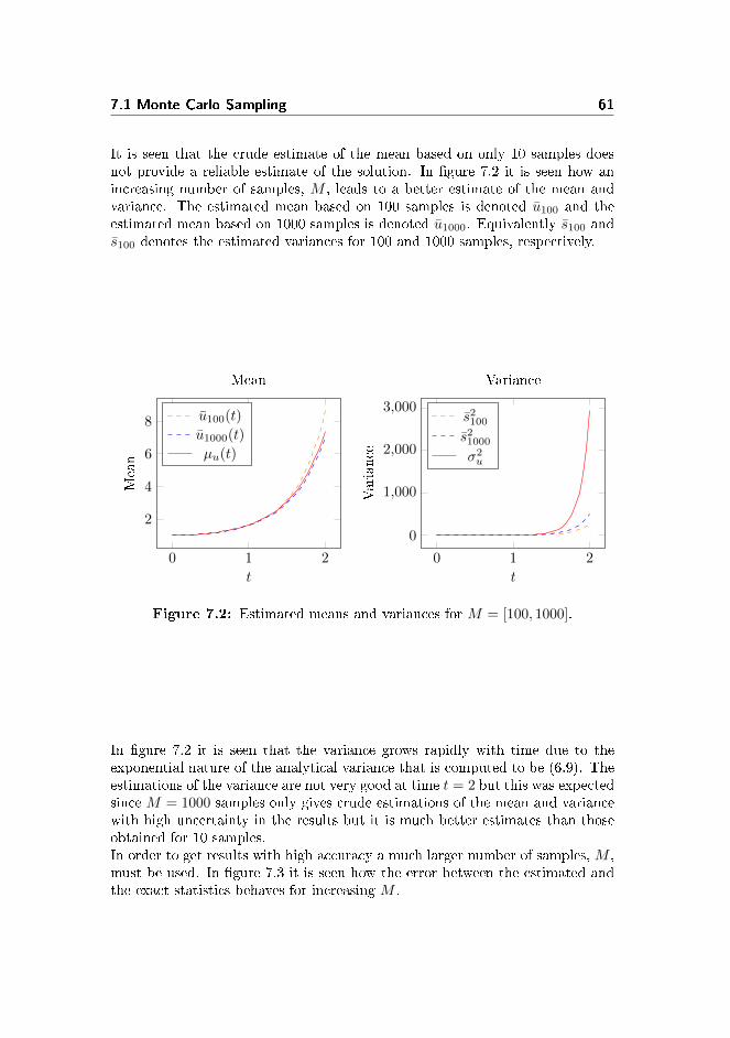
7.1 Monte Carlo Sampling 61
It is seen that the crude estimate of the mean based on only 10 samples doesnot provide a reliable estimate of the solution. In gure 7.2 it is seen how anincreasing number of samples, M , leads to a better estimate of the mean andvariance. The estimated mean based on 100 samples is denoted u100 and theestimated mean based on 1000 samples is denoted u1000. Equivalently s100 ands100 denotes the estimated variances for 100 and 1000 samples, respectively.
0 1 2
2
4
6
8
t
Mean
Mean
u100(t)
u1000(t)
µu(t)
0 1 2
0
1,000
2,000
3,000
t
Variance
Variance
s2100
s21000
σ2u
Figure 7.2: Estimated means and variances for M = [100, 1000].
In gure 7.2 it is seen that the variance grows rapidly with time due to theexponential nature of the analytical variance that is computed to be (6.9). Theestimations of the variance are not very good at time t = 2 but this was expectedsince M = 1000 samples only gives crude estimations of the mean and variancewith high uncertainty in the results but it is much better estimates than thoseobtained for 10 samples.In order to get results with high accuracy a much larger number of samples, M ,must be used. In gure 7.3 it is seen how the error between the estimated andthe exact statistics behaves for increasing M .
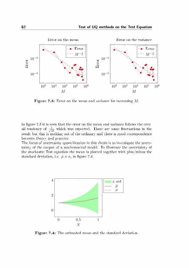
62 Test of UQ methods on the Test Equation
102 103 104 105 106
10−4
10−3
M
Error
Error on the mean
Error
M−12
102 103 104 105 106
10−4
10−3
M
Error
Error on the variance
Error
M−12
Figure 7.3: Error on the mean and variance for increasing M .
In gure 7.3 it is seen that the error on the mean and variance follows the over-all tendency of 1√
Mwhich was expected. There are some uctuations in the
result but this is nothing out of the ordinary and there is good correspondencebetween theory and practice.The focus of uncertainty quantication in this thesis is to investigate the uncer-tainty of the output of a mathematical model. To illustrate the uncertainty ofthe stochastic Test equation the mean is plotted together with plus/minus thestandard deviation, i.e. µ± σ, in gure 7.4.
0 0.5 1
0
2
4
N
± stdµµ
Figure 7.4: The estimated mean and the standard deviation.
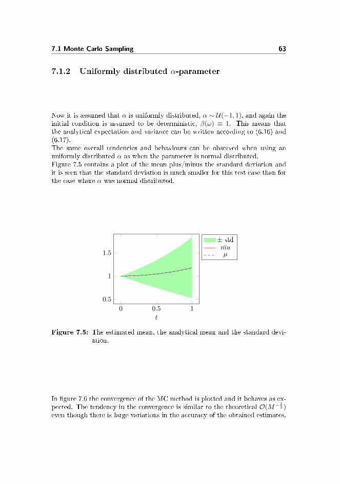
7.1 Monte Carlo Sampling 63
7.1.2 Uniformly distributed α-parameter
Now it is assumed that α is uniformly distributed, α ∼ U(−1, 1), and again theinitial condition is assumed to be deterministic, β(ω) ≡ 1. This means thatthe analytical expectation and variance can be written according to (6.16) and(6.17).The same overall tendencies and behaviours can be observed when using anuniformly distributed α as when the parameter is normal distributed.Figure 7.5 contains a plot of the mean plus/minus the standard deviation andit is seen that the standard deviation is much smaller for this test case than forthe case where α was normal distributed.
0 0.5 1
0.5
1
1.5
t
± stdmuµ
Figure 7.5: The estimated mean, the analytical mean and the standard devi-ation.
In gure 7.6 the convergence of the MC method is plotted and it behaves as ex-pected. The tendency in the convergence is similar to the theoretical O(M−
12 )
even though there is large variations in the accuracy of the obtained estimates.

64 Test of UQ methods on the Test Equation
102 103 104 105 106
10−4
10−3
10−2
10−1
M
Error
Mean
Error
M−12
102 103 104 105 106
10−4
10−3
10−2
10−1
MError
Variance
Error
M−12
Figure 7.6: Error on the mean and variance for increasing M .
7.2 Stochastic Collocation Method
From the theory it is known that the Stochastic Collocation Method shouldbe much more ecient than the Monte Carlo sampling for the 1D test case.Therefore the Stochastic Collocation Method (SCM) will be used on the sameproblem as before in order to check whether it delivers good results and if it ismore ecient.The application of the SCM for the Test Equation when α is the only stochasticparameter is outlined in algorithm 5.
Algorithm 5 Pseudocode for SCM applied to the Test Equation
1: Compute N + 1 quadrature nodes [zi]Ni=0 and weights [wi]
Ni=0.
2: Compute [αi]Ni=0 from [zi]
Ni=0
3: Solve the deterministic system to obtain the N + 1 deterministic solutions[ui]
Ni=0.
4: Compute the mean E[u] =∑Ni=0 uiwi
5: Compute the variance var(u) =∑Ni=0
(ui − E[u]
)2wi.
Which quadrature nodes and weights to be used depends on the distribution ofα as outlined in the theory. The deterministic solutions can be found by useof an appropriate solver in time - e.g. a Runge-Kutta method. The mean andvariance are computed as stated in the pseudocode and other statistics could becomputed as well.

7.2 Stochastic Collocation Method 65
7.2.1 Implementation
In this section some of the implementations used for SCM for Test Equationare introduced. The computation of the quadrature nodes and weights areimplemented as
1 i f strcmp (DistType , ' normal ' )2 % Gaussian D i s t r i bu t i on : Hermite Gauss Quadrature .3
4 [ z ,zW] = HermiteQuadN(zN) ; % Computing nodes andweights
5
6 z = mu+sigma∗z ; % Computing the alpha−parameter7 n = 0 : zN−1;8 e l s e i f strcmp (DistType , ' uniform ' )9 % Uniform Di s t r i bu t i on : Legendre Gauss Quadrature .
10
11 [ z ,zW] = legendrequad (zN) ; % Computing nodes andweights
12 zW = 1/2∗zW;13 end
where zN refers to the number of nodes in alpha. The implementation of thequadrature functions can be found in appendix B.The deterministic solutions are computed by using the Runge-Kutta methodERK.m. The deterministic solution is computed by
1 f o r t i = 1 : l ength ( tspan )−12 U( : , t i +1) = ERK( tspan ( t i ) ,U( : , t i ) ,@rhsSCMtest , dt , z ) ;3 end
where rhsSCMtest is the right-hand-side function implemented as
1 f unc t i on un = rhsSCMtest ( t ,U, alpha )2
3 un = alpha .∗U;
The statistics and the exact solutions have been computed as described in thetheory and the implementation can be found in appendix B as well as the im-plementation of a test script.

66 Test of UQ methods on the Test Equation
7.2.2 Gaussian distributed α-parameter
In this section the α-parameter is chosen to be standard normal distributed,α ∼ N (0, 1), which means that the Gauss Hermite quadrature rules have beenapplied to compute the appropriate quadrature nodes and weights. The errorsin mean and variance have been computed as a function of N , where N is thenumber of quadrature nodes and thereby the number of deterministic solutions.These errors can be seen in gure 7.7, where it is seen that the error of theestimated mean is not improving when more than 9 quadrature nodes are used.The error of the estimated variance requires more quadrature nodes to reach itsminimum at about 10−8 and reaches this minimum when 15 quadrature nodesare used. This means that the SCM reaches its best approximation of the meanwith 9 quadrature nodes and of the variance with 15 quadrature nodes at timet = 1. This is remarkably faster than when using the Monte Carlo Sampling.
100 101
10−10
10−5
100
N
Error
MeanVariance
Figure 7.7: Error on the mean and variance for increasing N , at time t = 1.
To indicate the uncertainty in the results the mean can be plotted together withthe standard deviation as was seen in gure 7.4 and gure 7.5. The computedmean and standard deviation are plotted in gure 7.8 as along with a plot ofthe deterministic solutions.

7.2 Stochastic Collocation Method 67
0 0.5 1
0
50
100
t
u(t
)Deterministic solutions
0 0.5 1
0
5
t
Statistics
± stdµ
Figure 7.8: Left: The deterministic solutions. Right: The mean estimatedand standard deviation.
From gure 7.8 it is seen that for time t = 1 there is a lot of uncertainty in theresult. This uncertainty would be increased in time since the variance increasesexponentially in time.
7.2.3 Uniformly distributed α-parameter
In this section it will be investigated how good the SCM is to estimate thestatistics when an uniform distributed α-parameter, α ∼ U(−1, 1), is used.In gure 7.9 the errors in mean and variance are plotted as function of thetotal number of nodes M and it seen that also for an uniformly distributedα-parameter the estimates will stabilize - this time at about 8.4 · 10−13 and2.8 · 10−12 for the mean and variance, respectively.

68 Test of UQ methods on the Test Equation
100 101
10−10
10−5
100
N
Error
MeanVariance
Figure 7.9: Error on the mean and variance for increasing N .
From gure 7.9 it is seen that for 7 quadrature nodes the error in the mean isminimized and equivalently for the variance for 8 quadrature nodes. This diersfrom the results obtained for a normal distributed α-parameter and it seems likethe choice of distribution eects both the statistics and the eciency of SCM.In gure 7.10 9 deterministic solutions and the corresponding mean and varianceare plotted.
0 0.5 1
1
2
t
Solutions
Deterministic solutions
0 0.5 1
0
0.5
1
1.5
t
Mean
Statistics
± stdµ
Figure 7.10: Left: The deterministic solutions. Right: The estimated meanand standard deviation.
Hence the SCM is more ecient than the MC and obtains quite good resultsfor even for a small number of deterministic solutions.

7.3 Stochastic Galerkin Method 69
7.3 Stochastic Galerkin Method
It is interesting to see how well an intrusive gPC Galerkin Method works com-pared to the MC method and the SCM. From the theory it is clear that forcomplicated problems this method can be very cumbersome to apply, since itrequires a lot of analytical derivation and extra implementations. However forthe simple Test equation this does not pose problem.The stochastic parameter α can be represented by the following univariate gPCprojection.
αN (Z) =
N∑i=0
aiΦi(Z), (7.1)
where the coecients ai are to be determined. Similarly can the initial conditionβ be represented by a gPC projection.
βN (Z) =
N∑i=0
biΦi(Z),
where bi are the coecients. The gPC approximation, vN , of the solution u isformulated as
vN (t, Z) =
N∑j=0
vjΦj(Z),
It is assumed that that α is stochastic and β is deterministic. Applying the gPCGalerkin procedure leads to
E[dvN
dtΦk
]= E
[−αNvNΦk
], k = 0, . . . , N. (7.2)
By substituting the expressions for vN and αN into (7.2) and evaluating theexpectations the following result is obtained.
dvNdt
= − 1
γk
N∑i=0
N∑j=0
aivjeijk, k = 0, . . . , N, (7.3)
where γk = E[Φ2k] and eijk = E[Φi(Z)Φj(Z)Φk(Z)] with 0 ≤ i, j, k ≤ N . The
orthogonality of the gPC basis polynomials is utilized when computing the left-hand side of (7.2). Usually γk is computable or at hand when choosing basisfunctions Φ but an expression for ei,j,k is not always at hand which means thatquadrature rules at times are used for approximating this constant.The system (7.3) can be represented by use of vector notation,
dv
dt(t) = ATv, v(0) = b,

70 Test of UQ methods on the Test Equation
where b = (b0, . . . , bN )T is the deterministic initial condition and the matrix Ais dened by A = (Aij)∀j,k, where Aij is dened by
Aij = − 1
γk
N∑j=0
aieijk.
This means that A is a (N + 1)× (N + 1) matrix. The system (7.3) is a systemof N + 1 ordinary dierential equations for the unknown coecients vk withinitial condition vk(0) = bk. A pseudocode for the implementation of the gPCGalerkin Method can be seen in algorithm 6.
Algorithm 6 Pseudocode for SGM applied to the stochastic Test Equation
1: Compute the initial condition b.2: Compute the coecient vector a.3: Compute the matrix A.4: Use a deterministic solver to solve system in time and hereby obtaining a
solution vector U .5: The mean is contained in the rst column of the solution U .6: Compute variance var(u) =
∑Ni=1
1γiU2i wi.
Here Ui refers to the i'th column of the solution U .
7.3.1 Implementation
The computation of the initial condition and the coecient vector follows thetheory described previously and the implementation can be seen in appendix B.The computation of the matrix A is implemented as
1 A = zero s (N+1,N+1) ;2 f o r j = 0 :N3 f o r k=0:N4 [ e , gamma] = TestGalPar ( j , k ,N) ;5 A( j +1,k+1) = −1/gamma∗( a '∗ e ) ;6 end7 end
where TestGalPar is implemented as
1 f unc t i on [ e , gamma] = TestGalPar ( j , k ,N)2

7.3 Stochastic Galerkin Method 71
3 % Pre−a l l o c a t i o n4 e = ze ro s (N+1 ,1) ;5
6 % Computation o f a vec to r conta in ing the e−va lue s .7 f o r i = 0 :N8 s = ( i+j+k) /2 ;9
10 i f s<i | | s<j | | s<k | | mod( ( i+j+k) ,2 )~= 011 e ( i +1) = 0 ;12 e l s e13 e ( i +1) = f a c t o r i a l ( i ) ∗ f a c t o r i a l ( j ) ∗ f a c t o r i a l ( k )
. . .14 /( f a c t o r i a l ( s−i ) ∗ f a c t o r i a l ( s−j ) ∗
f a c t o r i a l ( s−k ) ) ;15 end16 end17
18 % Computation o f the norma l i za t i on f a c t o r gamma.19 gamma = f a c t o r i a l ( k ) ;
The deterministic system is solved by use of the implemented function ERK.
7.3.2 Gaussian distributed α-parameter
Now the α-parameter is assumed to be Gaussian distributed, α ∼ N (µ, σ),which implies that the gPC basis, ΦkNk=0, is chosen to be Hermite polynomials,Hk(Z)Nk=0, and Z ∼ N (0, 1). Since α can be represented as α = µ + σZ thegPC representation (7.1) can be expressed as
αN (Z) =
N∑i=0
aiHi(Z),
where a0 = µ
a1 = σ
ai = 0 i ≥ 2
(7.4)
In this case αN is an exact representation of α for N ≥ 1 which is not alwaysthe case. Furthermore vN can be represented as
vN (t, Z) =
N∑i=0
viHi(Z).

72 Test of UQ methods on the Test Equation
By using Hermite polynomials the constants in (7.3) can be expressed asγk = k! k ≥ keijk = i!j!k!
(s−i)!(s−j)!(s−k)! s ≥ i, j, k and 2s = i+ j + k is even.(7.5)
The convergence of the estimated mean and variance is illustrated by plottingthe errors as functions of N as seen in gure 7.11.
100 101
10−7
10−3
101
N
Error
MeanVariance
Figure 7.11: Error of the estimated mean and variance for increasing N .
It is seen that for the SCM 6 and 10 basis polynomials are needed for obtain-ing the minimum error of the estimated mean and variance respectively. Thenumber of polynomials used also corresponds more or less to the number ofdeterministic solutions that have to be computed. This means that the SGMresults in slightly less deterministic solutions to be computed than the SCM. Itis however worth to note that for this test case, the rhs of the SCM is simplerand faster to evaluate than the rhs for the SGM.
7.3.3 Uniformly distributed α-parameter
Now the α parameter is assumed to be uniformly distributed, α ∼ U(a, b), witha = −1 and b = 1. This means that another the gPC basis, ΦkNk=0, has tobe used, namely Legendre polynomials, Lk(Z)Nk=0 with Z ∼ U(a, b). The ap-proximation of α can be expressed by an expansion with Legendre polynomials,L(Z), as
αN (Z) =
N∑i=0
aiLi(Z),

7.4 Conclusion 73
where a0 = b+a
2 ,
a1 = b−a2 ,
ai = 0 i ≥ 2.
(7.6)
Again αN is an exact representation of α for N ≥ 1. The representation of vN
can with Legendre polynomials be expressed as
vN (t, Z) =
N∑i=0
viLi(Z).
By using Legendre polynomials the constants in (7.3) can be expressed as γk =2
2k+1 and eijk is approximated by Gauss Legendre quadrature.The convergence plot can be seen in gure 7.12.
100 10110−11
10−6
10−1
N
Error
MeanVariance
Figure 7.12: Error on the mean and variance for increasing N .
It is seen that 5 and 6 polynomials are needed for obtaining the minimum errorof the estimated mean and variance respectively. Again this is slightly less thanfor the SCM but with this simple test case the dierence in eciency is notthat important since both are very fast and easily evaluated. The SGM doeshowever require a little more analytical work and some more implementation.
7.4 Conclusion
In this section it has been established that it is possible to obtain good esti-mates of the statistics with all three methods. Furthermore the Monte Carlomethod has a convergence rate which ts the theoretical M−
12 and the SCM

74 Test of UQ methods on the Test Equation
and SGM shows spectral convergence. The numerical tests conducted in thissection demonstrates why the spectral methods are an attractive tool to use inthe context of UQ.

Chapter 8
Burgers' Equation
Burgers' equation has been described previously and with a stochastic leftboundary condition it can be formulated as (6.23). In this chapter the re-sults from the numerical tests with the stochastic Collocation method and thestochastic gPC Galerkin method will be presented. In the following it will be as-sumed that δ(Z) ∼ U(−1, 1) and thus the polynomials used in the gPC Galerkinmethod will be Legendre polynomials and the collocation points and weights willbe computed from a Gauss Legendre quadrature.
8.1 Stochastic gPC Galerkin method
In order to apply the Galerkin method a one dimensional gPC expansion isformulated as
vN (x, t, Z) =
N∑j=0
vj(x, t)Φj(Z). (8.1)
This expansion is substituted into (6.23) and the Galerkin procedure is appliedwhich leads to
E[∂vN
∂tΦk
]+ E
[vN
∂vN
∂xΦk
]= νE
[∂2vN
∂x2Φk
], k = 0, . . . , N. (8.2)

76 Burgers' Equation
By substituting with the expression (8.1) for vN the orthogonality of the basisfunctions can be applied. This means that the rst term in the left-hand-side(lhs) of (8.2) can be rewriting as
E[∂vN
∂tΦk
]= E
N∑j=0
∂vj∂t
ΦjΦk
(8.3)
=N∑j=0
∂vj∂t
E [ΦjΦk]
=
N∑j=0
∂vj∂t
γkδj,k
=∂vk∂t
γk,
where δj,k is the Kronecker delta function and γk = E[Φ2k
]. The non-linear
term in the lhs can be rewriting as
E[vN
∂vN
∂xΦk
]= E
N∑i=0
viΦi
N∑j=0
∂vj∂x
ΦjΦk
(8.4)
= E
N∑i=0
N∑j=0
vi∂vj∂x
ΦiΦjΦk
=
N∑j=0
N∑i=0
vi∂vj∂x
E [ΦiΦjΦk]
=
N∑i=0
N∑j=0
vi∂vj∂x
ei,j,k,
where ei,j,k = E [ΦjΦiΦk]. The rhs of (8.2) can be rewriting as
νE[∂2vN
∂x2Φk
]= νE
N∑j=0
∂2vj∂x2
ΦjΦk
(8.5)
= ν
N∑j=0
∂2vj∂x2
E [ΦjΦk]
= ν
N∑j=0
∂2vj∂x2
γkδj,k
= ν∂2vk∂x2
γk
8.1 Stochastic gPC Galerkin method 77
This means that the system can be dened as
∂vk∂t
+1
γk
N∑i=0
N∑j=0
vi∂vj∂x
ei,j,k = ν∂2vk∂x2
, k = 0, . . . , N. (8.6)
8.1.1 Numerical approximations
This section contains a description of how to approximate dierentiation in spaceand time numerically. In space there will be used central dierence schemes andin time an explicit four step Runge-Kutta method will be applied. The centralapproximation for dierentiation in space is given as
∂
∂xu(xi, tj) =
u(xi+1, tj)− u(xi−1, tj)
2δx,
where δx is the distance between the points in the space grid. The second orderderivative is estimated by the following 3-point central dierence approximation
∂2
∂x2u(xi, tj) =
u(xi+1, tj) + u(xi−1, tj)− 2u(xi, tj)
δ2x
.
In both central approximations it has been assumed that the space grid pointsare equidistant. If this is not the case the 2δx and δ2
x should be replaced with|xi − xi−1|+ |xi+1 − xi| and |xi − xi−1||xi+1 − xi|, respectively.
These central dierence approximations leads to the following stencils
Adx =1
2δx
−1 0 1 00 −1 0 1 0
. . .. . .
0 −1 0 1
(8.7)
and
Adx2 =1
δ2x
1 −2 1 00 1 −2 1 0
. . .. . .
. . .
0 1 −2 1
(8.8)
There is Nx + 1 space points and N + 1 polynomials in the expansion. In orderto cope with the multiple sums in (8.6) a Kronecker product can be used toobtain the following matrices
78 Burgers' Equation
Ak =
e0,0,kAs e0,1,kAs · · · e0,N,kAse1,0,kAs e1,1,kAs · · · e1,N,kAs
.... . .
...eN,0,kAs eN,1,kAs · · · eN,N,kAs
and Bk =1
δ2x
−2 1 01 −2 1 0
. . .. . .
. . .
11 −2
,
where
As =1
2δx
0 1 0−1 0 1 0
. . .. . .
0 1−1 0
By introducing these matrices the system (8.6) can be written as
∂vk∂t
= νBkv −1
γkvAkV + gk, k = 0, . . . , N. (8.9)
where V and v are all the interior points of v and gk is a vector added to thesolution to apply the boundary condition and is dened as
gk =
1δ2xv0k + 1
γk1
2δx
∑Ni=0
∑Nj=0 v
0i v
0j ei,j,k
0...0
1δ2xvNxk − 1
γk1
2δx
∑Ni=0
∑Nj=0 v
Nxi vNxj ei,j,k
,
where v0k is the left boundary point of the k'th expansion and vNxk is the right
boundary point of the k'th expansion. The matrix V and the vector v can berepresented as
V =
v1,0 . . . v1,N 00 v2,0 . . . v2,N 0
. . .. . .
. . . 0 v2,0 . . . v2,N
and v =
v1,0
v2,0
...vNx−1,0
v1,1
...vNx−1,1
v1,2
...vNx−1,N
.

8.1 Stochastic gPC Galerkin method 79
The computation of the IC is outlined in the next section about the imple-mentation. To solve the problem the implemented ERK-method is used andpost-processing consists of computing the interesting statistics from the com-puted solution.The SGM for Burgers equation is outlined in the pseudocode in algorithm 7.
Algorithm 7 Pseudocode for SGM applied to the stochastic Burgers Equation
1: Compute the points in space x.2: Compute the initial condition.3: Solve the system in time (reach steady state).4: Compute the mean E[u] = U0
5: Compute the variance var(u) =∑Ni=1 γi(Ui)
2.
8.1.2 Implementation
All the implementations for SGM used on Burgers' equation can be found inappendix and in this section some of the the implementation are introduced.First the implementation of the initial condition is outlined and it yields
1 % Mean and standard dev i a t i on .2 b_mean = (1.1−1) /2 ; std = sq r t (1/12∗(1.1−1) ^2) ;3
4 % Boundary cond i t i on s5 b1 = 1+b_mean ; b2 = −1;6
7 v=−x ;8 v (1 )=b1 ; v (xL)=b2 ;9
10 % I n i t i a l cond i t i on f o r a l l N11 U1 = ze ro s ( ( xL−2)∗(N+1) ,1 ) ;12 U1( 1 : xL−2)=v ( 2 : xL−1) ;
The initial condition is established by computing a zero-vector U1 of length(N + 1) · (Nx− 2) which corresponds to having a space vector containing all theinterior points for each of the N + 1 polynomials.This vector is modied by replacing the rst Nx − 2 elements with the interiorspace points with reversed sign.A test script have been implementation and can be seen in appendix B. Thisimplementation relies heavily on the rhs-function rhsGalBurg which get thecurrent solution and the matrices described in the previous section as input and

80 Burgers' Equation
then computes (8.9). The implementation is seen in appendix B.The computations outlined in this section have been based on computing thesolution in each time step for the interior points. To compute the values inthe end points for each of the N terms in the gPC expansion the followingimplementation is applied
1 U = zero s ( s i z e ( v ) ) ;2 f o r iB = 0 :N3 U(xL∗ iB+1) = b1 ;4 U(xL∗( iB+1) ) = b2 ;5 U(xL∗ iB+2:xL∗( iB+1)−1) = U1( ( xL−2)∗ iB+1:(xL−2)∗( iB+1)
) ;6 end
where U1 refers to the computed solution in the interior points and b1 and b2
refers to the values in the left and right boundary, respectively.
8.1.3 Numerical experiments
When solving Burgers' equation a steady state solution has to be obtained -this holds for both the deterministic and stochastic case. As an illustration thedeterministic Burgers' equation is solved with initial condition −x for dierenttimes.
−1 0 1
−1
0
1
x
Solutions
Figure 8.1: The computed solutions for dierent bounds on the integration intime.
It is seen that the further out in time the deterministic system is solved thecloser it comes to the steady state solution which was plotted in gure 6.1.The SGM has been used in a setting with Nx = 41 space points and with

8.2 Stochastic Collocation Method 81
N + 1 = 4 terms in the gPC expansion. The estimated mean and variancehave been plotted in gure 8.2. These statistics have been plotted togetherwith upper and lower bounds on the deterministic solutions and the standarddeviation has been plotted around the mean to indicate the uncertainty in themean.
−1 0 1
−1
0
1
x
StdVarµ
Bound
Figure 8.2: The mean, variance and bounds for the computed solution.
The statistics have naturally been computed such that steady state is reached.
8.2 Stochastic Collocation Method
The stochastic Collocation method is applied to the stochastic Burgers' equa-tion. As mentioned earlier the collocation points and weights used for are com-puted by use of Gauss Legendre quadrature and the used deterministic solveris the ERK-method in combination with a deterministic spectral Collocationmethod for solving the spatial part of the PDE.As described earlier a deterministic Collocation method can involve computingdierential matrices in order to handle the dierentiation in space. To handlethis a set of deterministic collocation points has to be chosen and the Vander-monde matrices V and Vx has to be computed.This setup means that there will be two sets of collocation points involved -the stochastic Gauss Legendre collocation points z and the deterministic GaussLobatto collocation points, x.The polynomials used in the Vandermonde matrices V and Vx are Legendre

82 Burgers' Equation
polynomials which means that the matrices can be expressed as
V =
L1(x1) L1(x2) · · · L1(xN )L2(x1) L2(x2) · · · L2(xN )
......
. . ....
LN (x1) LN (x2) · · · LN (xN )
and
Vx =
L1(x1)′ L1(x2)′ · · · L1(xN )′
L2(x1)′ L2(x2)′ · · · L2(xN )′
......
. . ....
LN (x1)′ LN (x2)′ · · · LN (xN )′
.From the theory it is known that the dierentiation matrix can be expressedas D = VxV−1. This means that a discrete representation of Burgers equation(6.22) can be expressed as
∂u
∂t= νD2u− uDu, x ∈ [−1, 1] , (8.10)
The rhs function either consists of a loop that does the matrix vector multipli-cation for each i = 1, . . . , Nz, that is
νD2ui − uiDui, i = 1, . . . , Nz
or by constructing two big, sparse matrices Dkron and D2kron that are the com-
puted by taking the Kronecker product between an identity matrix of appropri-ate size and D and D2, respectively. This leads to a rhs function that does thefollowing computation
νD2kronu− uDkronu
The post-processing of the deterministic solutions follows from the theory andthe statistics are computed as seen in Algorithm 8 that outlines SCM For Burg-ers' equation.
Algorithm 8 Pseudocode for SCM applied to the stochastic Burgers' equation
1: Compute the collocation points x.2: Compute the parameters for the rhs, i.e. D and D2.3: Compute the initial condition IC and quadrature weights w.4: Use a deterministic solver to solve the system in time (reach steady state).
5: Compute the mean E[u] =∑Ni=0 uiρwi
6: Compute the variance var(u) =∑Ni=0
(ui − E[u]
)2ρwi.
All the code for SCM for Burgers' equation can be seen in Appendix B and themost important parts are outlined in the following section.

8.2 Stochastic Collocation Method 83
8.2.1 Implementations
The collocation points are computed by use of quadrature and the implemen-tation can be seen in Appendix B. The implementation of the Vandermonde-matrices and the dierentiation matrices are also included in the appendix. Theinitial condition is implemented as
The stochastic collocation points, z, are used for computing an initial condition.The implementation can be found in Appendix B. The deterministic solutionsare computed in the Matlab function BurgDetSolv which is implemented as
1 f unc t i on [U, t , time ] = BurgDetSolv (U, dt , param , ErrorBar ,MaxIter )
2
3
4 t = ze ro s (MaxIter , 1 ) ;5
6 i t e r = 0 ;7 d i f f = 1 ;8
9 t i c10 whi le d i f f > ErrorBar && i t e r <= MaxIter11 UTemp = U;12 U = ERK( t ( i t e r +1) ,U, @rhsColBurg , dt , param) ;13 t ( i t e r +2) = t ( i t e r +1)+dt ;14 d i f f = max( abs (UTemp−U) ) ;15 i t e r = i t e r +1;16 end17 time = toc ;
It is seen that the deterministic solutions are computed by using a while-loopwhere the function ERK is called in each iteration.The while-loop is used to ensure that a state "close" to the steady state isreached. The assumption is that the less change in the computed solutions thecloser are the solutions to steady state and the dierence between two consec-utive solutions is therefore used as a measure for how close to steady state thecurrent solution is.The boundary conditions are applied in the rhs-function by setting the end-point values for each solutions to zero. The implementation of the rhs is seenin appendix B as well as the rest of the implementations.
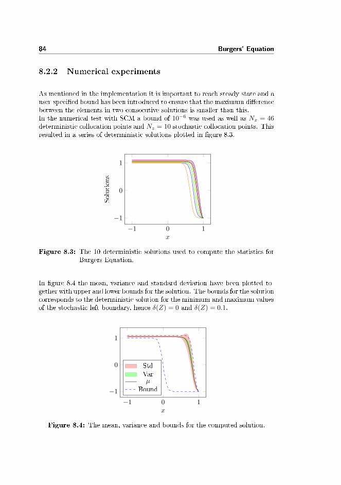
84 Burgers' Equation
8.2.2 Numerical experiments
As mentioned in the implementation it is important to reach steady state and auser-specied bound has been introduced to ensure that the maximum dierencebetween the elements in two consecutive solutions is smaller than this.In the numerical test with SCM a bound of 10−6 was used as well as Nx = 46deterministic collocation points and Nz = 10 stochastic collocation points. Thisresulted in a series of deterministic solutions plotted in gure 8.3.
−1 0 1
−1
0
1
x
Solutions
Figure 8.3: The 10 deterministic solutions used to compute the statistics forBurgers Equation.
In gure 8.4 the mean, variance and standard deviation have been plotted to-gether with upper and lower bounds for the solution. The bounds for the solutioncorresponds to the deterministic solution for the minimum and maximum valuesof the stochastic left boundary, hence δ(Z) = 0 and δ(Z) = 0.1.
−1 0 1
−1
0
1
x
StdVarµ
Bound
Figure 8.4: The mean, variance and bounds for the computed solution.

8.2 Stochastic Collocation Method 85
It is seen from gure 8.4 that the solution of Burgers' equation is very sensitivetowards disturbances in the boundary since the transition layer moves quite alot. The upper and lower bounds gives a good impression of the span of thesolution when the boundary is disturbed with between 0 and 10 percent noise.The steady-state estimation of the mean is also quite dierent from the unper-turbed solution (the lower bound) and this illustrates that even though errorson the estimations are small and the estimated variance is relatively small aswell, the computed statistics does not give an especially good impression of thenoise-free solution.It is worth to note that this is another dimension to the UQ analysis. Thereare errors on the computed estimates and when the estimates are accurate thevariance might be very large and thereby make the solutions very uncertain.Furthermore if UQ is conducted to get an impression of the unperturbed deter-ministic solution it should be noted that the computed statistics might deviatea lot from this solution.

86 Burgers' Equation
Chapter 9
Discussion: Choice ofmethod
The methods used in this thesis is the Monte Carlo Sampling, the stochasticGalerkin method and the stochastic Collocataion method and these will in thefollowing be compared.From the outlined theory and the numerical experiments it is clear that theMonte Carlo sampling has relatively slow convergence compared to the twoother methods for low dimensional problems and it can be cumbersome to usewhen the deterministic system is very time consuming to solve.It is however an interesting method since it can be used as a reference whenexploring new problems and since its convergence rate is independent of thenumber of stochastic variables. As mentioned in the theory the computationaleort of the stochastic gPC Galerkin method and especially of the stochasticcollocation method grows rapidly as the number of stochastic variables in thesystem is increased. This means that at a certain point the Monte Carlo Sam-pling will become more ecient than the two spectral methods.The dierence in accuracy is also one of the distinctions between the Galerkinmethod and the Collocation method. The Galerkin method is based on minimis-ing the residue of the stochastic governing equations. The collocation methodis based on a dierent approach namely to introduce a set of nodes and ensurethat the error in these nodes are zero. When using this approach there willbe problems with aliasing errors which means that the collocation method ingeneral is less accurate than the Galerkin method. This is especially true for

88 Discussion: Choice of method
multidimensional spaces. In the univariate case the aliasing error can be keptat the same order as the nite order Galerkin method [19].This means that based on an accuracy perspective the Galerkin method is tobe preferred over the Collocation method but there is another important aspectnamely the implementation.The Galerkin method implies derivation of a gPC Galerkin system where theequations for the expansion coecients are coupled. This usually means thatnew implementations have to be made in order to cope with the coupled sys-tems. Furthermore the derivation of the gPC equations can be very tricky andin some cases it is not possible to make the derivations [19].This is very dierent from the Collocation method where the deterministic sys-tems solved for each node are decoupled and could be solved with parallel pro-gramming [19]. The Collocation method is relatively easy to implement as longas there exists decent deterministic solvers for the problem at hand. Whenthis criteria is fullled the Collocation method can be boiled down to choosingthe set of collocation nodes, solve the deterministic problem at each node andperform post-processing by applying either the interpolation approach or thediscrete projection approach described earlier.A consequence of this is that even though the original problem might be non-linear or complex problem it is still relative straight forward to solve as longas a deterministic solver is at hand or can be derived. This means that theCollocation method might be less accurate than the Galerkin method but it ismuch easier to apply and for this reason the Collocation method is very popular.
The Galerkin method is the most accurate and involves the least number ofequations in a multidimensional space. But the Collocation method is mucheasier to implement and the derivation of the gPC Galerkin equations can bevery dicult and even impossible in some cases [19]. This means that the choiceof method is not trivial since each method has its strengths and weaknesses andthe choice depends a lot on the dimensionality and complexity of the problem.
The SCM is interesting because of the ease of implementation and if the curseof dimensionality could be reduced it would be a useful tool in high dimensions.Therefore the rest of the thesis will involve the SCM for multivariate problems.
Chapter 10
Literature Study
As introduced in earlier the stochastic Collocation method has some nice proper-ties but it also has some drawbacks with regard to the amount of computationalwork. Due to this a literature study has been conducted with focus on how tooptimize the use of SCM.In section 10.1 a brief outline of the studied topics is given and in the followingsections of this chapter some of the topics are introduced more thoroughly.
10.1 Brief Introduction to topics and articles
Some of the eects of the curse of dimensionality can be reduced by use of sparsegrids instead of a full tensor product grid. The Smolyak grids are widely used inthe eld of UQ and they will be introduced later in the thesis. Some interestingwork worth noting is the MatLab scripts and the documentation in [14] and[13], respectively. This work makes it possible to easily access implementationof dierent sparse grids and to compare them. Furthermore the work of JohnBurkardt [2] with regard to Matlab implementation of the Gauss Legendresparse grid is also very useful as well as the work of Florian Heiss and ViktorWinschel [11] which contains implementation of Smolyak sparse grids. Inter-ested readers can learn more about the topic in e.g. [3], [5], [16] and [19].

90 Literature Study
The article [5] claims that the common way of using the sparse grids might notbe optimal and introduces another way of using the sparse grids such that theerrors in the coecients to the higher order polynomials are reduced. The newapproach is denoted Sparse Pseudospectral Approximation Method (SPAM) andis outlined in section 10.2.
Two articles introducing an interesting approach to minimize the size of thesystems to be solved and thereby avoiding the curse of dimensionality are [6]and [21]. In these articles an approach known from signal processing is appliedin the eld of Uncertainty Quantication.The approach is called Compressive Sensing - or Compressive Sampling - and isbased on constructing an approximation to the solution by use of an orthogonalprojection. The main idea is that this orthogonal projection in some cases willform a sparse system which can be utilized to minimize the computational eort[6]. The approach is outlined in section 10.3.A well-known topic from the statistical modelling is the analysis-of-variance(ANOVA) which also have been used in UQ. ANOVA is a method where the totalvariance is investigated by decomposing the original problem into subproblemsand then computing the variance for each subproblem. It is a method oftenused adaptively in UQ to reduce the computational work as in introduced in[9] or [22]. The interested reader can nd an overview of some relevant andrecent articles and topics within ANOVA for uncertainty quantication in theintroduction of [23] .
10.2 Sparse Pseudospectral Approximation Method
The method outlined here is described in the article [5] and it is an alterna-tive way of utilizing the sparse grid procedure introduced earlier. The alterna-tive procedure is introduced to avoid errors in the coecients of the high-orderpolynomials which is a result of the usual application of the Smolyak methodaccording to [5].The reason why these errors emerge is according to [5] that the coupling betweenthe nodal Lagrange representation and the modal polynomial representation inmultiple dimensions - which is described for the one-dimensional case in chapter2 - does not hold in the sparse settings.In 10.2.1 some notation and concepts are introduced and the new approach isoutlined in 10.2.2.
10.2 Sparse Pseudospectral Approximation Method 91
10.2.1 Introduction of notation and concepts
In this section some concepts and denitions from [5] are introduced. In thefollowing a pseudospectral projection refers to a projection where the integralsare approximated by numerical integration rules, e.g. quadrature rules. Inchapter 4 a truncated polynomial projection of a multivariate function f wasintroduced as
PNf(s) =
n1∑i1=1
· · ·nd∑id=1
fi1,...,idΦi1(s1) · · ·Φid(sd) =∑|i|∈Ii
fiΦi(s),
where s = (s1, . . . , sd) refers to a d-dimensional point, Ii = i | i ∈ Nd, 1 ≤ ik ≤nk, k = 1, 2, . . . , d is the set of admissible multi-index and fi are the coecientsdened as [5]
fi =1
γi
∫f(s)Φi(s)w(s)ds, ∀|i| ≤ N.
The pseudospectral projection is dened equivalently but the coecients aredened by use of numerical integration rules and yields
fi =
n1∑i1=1
· · ·nd∑id=1
f(λi1 , . . . , λid)Φi1(s1) · · ·Φid(sd)1
γi1· · · 1
γid
=∑|i|∈Ii
f(λi)Φi(λi)1
γi.
where λi refers to the chosen quadrature points. The article also refers to La-grange interpolation and introduces that the correspondence between the nodaland modal representations introduced in chapter 2 can be expanded to the mul-tidimensional case when using the tensor grid representations [5].
The approach of using the pseudospectral projection combined with the Smolyaksparse often consist of rst making the truncation of the spectral projection andthen compute the approximations of the coecients by use of a sparse gridquadrature rule [5]. According to [5] this leads to errors in the coecients be-cause with sparse grid integration the truncated pseudospectral approximationis not equivalent to the Lagrange interpolating polynomial as was the case whenusing the tensor product approximation.

92 Literature Study
10.2.2 Overall approach
The idea of sparse pseudospectral approximation method (SPAM) is that sincethe sparse grid is introduced as a linear combination of tensor product quadra-ture rules the same can be applied to compute a linear combination of tensorproduct pseudospectral expansions [5]. This is the concept of the sparse pseu-dospectral approximation.When introducing the Smolyak sparse grid a set of admissible indices I and acoecient function c(i) is introduced as well. The set I is dened as [5]
I = i ∈ Nd | l + 1 ≤ |i| ≤ l + d,
where l is an integer called the level parameter. The coecients can be denedas
c(i) = (−1)l+d−|i|(
d− 1l + d− |i|
).
These are used in SPAM as well. The approximation of a multivariate functionf(s) can be expressed as
f(s) ≈ Ap(f) =∑i∈I
c(i)fTi Φi(s).
where coecients fi and the polynomials Φi are dened as for the pseudospectralprojection introduced in section 10.2.1. The set of polynomials Φi(s) can beused to create a set of basis polynomials for Ap by dening
P =⋃i∈I
Φi(s).
With this denition of the basis the Ap(f) can be written as
Ap(f) =∑
Φi∈PfΦΦ(s),
where the coecients fΦ are formulated as
fΦ =∑i∈I
c(i)fi,m.
Furthermore the coecients fi,m are dened as
fi,m =
fi if Φ(s) = Φi(s) and i ∈ I0 otherwise.
In [5] there is a theorem stating that this approximation is equivalent to thesparse grid interpolation approximation and there are numerical experimentswhich indicates that SPAM might be better than the usual pseudospectral pro-jection approach when it comes to computing the coecients for the high orderpolynomials

10.3 Compressive sampling: Non-adapted sparse approximation of PDES93
10.2.3 Further reading
For a more thorough introduction to SPAM and the theory behind it the inter-ested readers are referred to the article [5]. The article also contains numericaltests that should illustrate the purpose and advantages of SPAM.
10.3 Compressive sampling: Non-adapted sparse
approximation of PDES
As mentioned previously in the literature study the compressive sampling is anapproach used in signal processing and recently it has been applied in the eldof UQ. The introduction given here is mainly based on the articles [6] and [21].Compressive sampling is an interesting and exible approach that is based onrepresenting the solution by an expansion and then utilize the sparsity of theexpansion.The main assumption is that the expansion is sparse in the sense that relativelyfew coecients are signicant such that an underdetermined system can repre-sent the actual system accurately or even exactly. It is an approach that is wellsuited for the cases where not enough data is available and for high dimensionalmultivariate problems.One of the very interesting aspects of the approach is that it is non-adaptedin the sense that there is no tailoring of the sampling process and thereby nostructuring of the nodes. This is an advantage since the structuring of the nodesis often what leads to a rapid growth in the total number of nodes when thedimensionality of the problem is increased.
10.3.1 Overall approach
The approach outlined here is based on approximation of the solution to asystem of the type outlined in 5.1. The approach outlined here is an interpo-lating collocation type of method and is based on constructing a multivariatepolynomial expansion that approximates the solution u(x, t, Z). The truncatedexpansion can be expressed as
uN =∑|i|≤N
uiΦi(Zm), m = 1, . . . ,M, (10.1)
where Z refers to the set of multivariate samples introduced in chapter 4, Φi(Z)are the multivariate polynomials also introduced in chapter 4 and the coecients

94 Literature Study
can be computed as
ui =1
γiE[uΦi] =
1
γi
∫u(z)Φi(z)dFZ(z), ∀|i| ≤ N.
by use of the multivariate expectation introduced previously.
Such a system can be expressed in vectorized form by introducing a Vander-monde like matrix V ∈ RP×M where M is the number of samples and P isthe cardinality of the space spanned by the orthogonal basis polynomials Φi(Z).The matrix V consists of Vn,m = Φin(Zm) for n = 1, . . . , P and m = 1, . . . ,M .This means that the vectorized representation is on the form
Vc = u,
where c ∈ RP is a coecient vector consisting of the coecients ui and u ∈ RMis a vector containing the solutions u(x, t, Zm) for each of the M samples of therandom variables.The main idea in the compressive sampling approach is to solve an under-determined system by use minimization to reduce the number of samples M .This means that the number of samples M is reduced to be far smaller thanthe cardinality P of the expansion, i.e. M P . The minimization acts as aregularization in order to achieve a well-posed solution to the underdeterminedsystem [6] and takes the form
min ‖c‖k subject to Vc = u (10.2)
where k = 0, 1. The norms used for the minimizations can be formulated as
‖c‖0 = #i : ui 6= 0 and ‖c‖1 =∑|i|≤N
|ui|
The minimization using k = 0 generally leads to a global minimum solutionwhich is not unique and where the cost of a global search is exponential in P[6]. The `1-minimization is a relaxation of the `0-minimization ([6], [21]) and isusually the one pursued in practice.Instead of using an interpolation strategy it can sometimes be useful to relaxthe constraints in the minimizations in the sense that some error is allowed
min ‖c‖0 subject to ‖Vc− u‖2 ≤ δ,min ‖c‖1 subject to ‖Vc− u‖2 ≤ δ.
This relaxation can be used for several reasons and one of them is that thetruncated expansion (10.1) often is not an exact representation of the solutionu(x, t, Z) due to truncation errors and this is reected in the minimizations byintroducing a non-zero residual [6].
10.3 Compressive sampling: Non-adapted sparse approximation of PDES95
10.3.1.1 Weighting of the `1-minimization
It is worth to note that the `1-minimization is sometimes modied by a diag-onal weight matrix W where the n'th diagonal element is the `2-norm of then'th column of V [6]. This means that the modied `1-minimization can beformulated as
min ‖Wc‖1 subject to Vc = u,
or in relaxed form
min ‖Wc‖1 subject to ‖Vc− u‖ ≤ δ.
The introduction of the weight W is to make sure that the optimization doesnot lead to a solution that is biased towards the c which are non-zero and whosecorresponding columns in V have a large norm [6].
10.3.2 Recoverability
This is only meant as a brief introduction and therefore most of the theoreticalbackground is not included here. Readers who are interested in the theoreticalbackground and the stability of the relaxed minimizations can read more in [6].One of the main results in [21] is the recoverability in the high dimensional cased 1 and d ≥ N where N is the highest polynomial order in one dimension ofthe polynomial basis. In order to introduce the result the following denitionof s-sparse is necessary [21].
Definition 10.1 (s-sparse) The vector v is called s-sparse if
‖v‖0 = #m : vm 6= 0 ≤ s,
which means that if there is no more than s non-zero elements in the vector vthen v is s-sparse.
The article [21] is based on a Legendre polynomial expansion which means thatthe main result cited in theorem (10.2) is based on Legendre polynomials but itcould be expanded to cover other polynomial bases as well [21].
Theorem 10.2 (Recoverability for `1-minimization) For d ≥ Nwhere d is the number of i.i.d. stochastic variables and N is the highest polyno-mial order in one dimension. Let Z be a sample of M independent draws fromthe uniform distribution [−1, 1]d. The number of samples M fulll the boundary
M ' 3P s log3(s)log(P )

96 Literature Study
where P is the cardinality of the polynomial space PdN introduced in chapter 4with d ≥ N and s is the sparsity level of a vector c ∈ RM . The Legendrepolynomials are chosen as basis polynomials for a polynomial approximationw ∈ PdN of the type 10.1 which yields
w(Z) =∑|i|≤N
uiΦi(Z),
where c is the coecient vector. This system is solved with regard to c by use of`1-minimization of the type (10.2) and the data vector u = Vc. For a universalconstant γ the introduced settings leads to c being recoverable with probability1− P−γ log3(s) to within a factor of its best s-term approximation, i.e.
‖c− c‖2 /δs,1(c)√
s(10.3)
where δs,p(v) = inf‖y‖0≤s ‖y−v‖p is the the error of the best s-term approxima-tion of a vector v ∈ RP in `p-norm.
The proof and theory behind theorem 10.2 can be found in [21].
10.3.3 Further reading
The outline of the method is given here and readers who are interested arerecommended to read more in [6] and [21]. The interested reader can besidesnumerical results and a more thorough introduction of the theoretical back-ground be introduced to Chebyshev Preconditioning of the `1-minimization in[21] and how to choose the truncation error tolerance δ in [6].The choice of δ is naturally an interesting topic when using the relaxed mini-mization and the Chebyshev preconditioning yields some interesting results aswell. For d ≥ P the preconditioning of the `1-minimization yields a numberof points that scales with 2d where the direct `1-minimization scales with 3P .This means that for large dimensions d and moderate polynomial order P thedirect minimization is the most ecient while in e.g. one dimension, d = 1, thepreconditioned `1-minimization is the most ecient.
Chapter 11
Multivariate CollocationMethod
In this chapter the theory for the stochastic collocation method will be expandedand the theoretical background for using a multivariate SCM is given. The in-troduced theory will be based on the interpolation approach of the collocationmethod.
11.1 Tensor Product Collocation
With the theory introduced so far the a straight forward approach for applyingSCM in multiple dimensions is to apply the univariate expansions in each ofthe stochastic dimensions and then use tensor products to combine these to amultivariate SCM.First a set of d ≥ 1 independent variables is introduced as Z = Z1, . . . , Zd andfor each variable a set ofmi collocation nodes is established as Zi = Z1
i , . . . , Zmii .
By use of Kronecker products this yields a total set of nodes Z dened as
Z = ZM = Z1 × · · · × Zdwhere M is the total number of nodes in the set and can be computed asM = m1× · · ·×md. The interpolating polynomial operator Imi in one variable

98 Multivariate Collocation Method
is introduced asImi [f ] =
∏mi
f(Zi) ∈ P(Zi). (11.1)
for 1 ≤ i ≤ d such that Imi [f ] is an interpolating polynomial of order mi in thei'th Z-variable equivalently to the univariate denition (5.2). This operator canbe used to construct the multivariate interpolation operator by tensor product
IM = Im1 ⊗ · · · ⊗ Imd
By using tensor products to expand the dimensionality of the space some ofthe properties from one dimension is valid for the multivariate case as well.This is true for the convergence rate as well. For simplicity but without loss ofgenerality it is here assumed that m1 = · · · = md = m. For the i'th dimensionthe one dimensional convergence rate is
(I − Imi)[f ] ∝ m−α,
where α is constant that depends on the smoothness of the function f - thesmoother a function the faster convergence, see e.g. [19]. This property stillholds in the multivariate case which yields the convergence rate
(I − IM )[f ] ∝ m−α.
It is a nice feature that this property holds in the multivariate case but apply-ing M = md and expressing the convergence rate in terms of M results in aconvergence rate of
(I − IM )[f ] ∝M−αd ,
This means that the convergence can be very slow if there is many stochasticvariables d. Furthermore the total number of points grows exponentially withd, i.e. M = md which means that the computational eort becomes very largefor large d. This is due to the fact that for each node a deterministic systemis solved, which could be very problematic in higher dimensions and is oftenreferred to as the curse of dimensionality [19].
11.2 Multivariate expansions and statistics
The multivariate SCM can be formulated in much the same way as the univariateSCM as will be outlined here. The interpolation of a solution u to a multivariatePDE with d stochastic variables can be formulated as
u(Z) ≡ IM (u) = (Im1⊗· · ·⊗Imd)(u) =
m1∑j1
· · ·md∑jd
u(Zj11 , . . . , Zjdd )(h1(Zj11 ) . . . hd(Z
jdd )),

11.2 Multivariate expansions and statistics 99
where hi refers to the Lagrange polynomial in i'th stochastic dimension. Thisnotation is widely adopted and is a bit more intuitive than the notation usingmulti-index. The multi-index and the corresponding single index does howeverallow a more compact notation, i.e.
IM (u) =∑|i|≤N
u(Zi)hi(Z),
where hi(Z) is the multidimensional Lagrange Polynomial in Z. By the de-nition of the multivariate Lagrange polynomials they have the same qualitiesas the univariate polynomials with regard to attaining zeros and ones in theinterpolation points.The connection between the univariate SCM and the multivariate SCM is easierseen when using the single index since the multidimensional interpolation canbe expressed as
IM (u) =
M∑k=1
u(Zk)hk(Z), (11.2)
where the correspondence between the multi-index and the single index is asoutlined in Table 4.1. The computation of the statistics, e.g. the expectationand the variance, can be conducted in much the same way as in the univari-ate case. The interested reader can read more about the application of themultidimensional cubature rules in [16], which leads to the following expression
Q(u) = (Q1 ⊗ · · · ⊗Qd)(u) =
m1∑j1
· · ·md∑jd
u(Zj11 , . . . , Zjdd )(ρ1w
j11 · · · ρdw
jdd ),
where Qi refers to the 1D quadrature applied in the i'th dimension, ρi is theintegration weight of the integral in the i'th dimension, i.e. the PDF of the i'thvariable Zi, and w
ji refers to the j'th quadrature weight of the i'th stochastic
variable.By use of the tensor product the notation can be simplied when an appropriateindex is used. The tensor product of the variables, Z, has already been intro-duced and likewise the weights can be expressed by use of a tensor product.First the weights wji = ρiw
ji are introduced to simplify notation and then the
tensor product is computed as
W = W1 ⊗ · · · ⊗Wd
where Wi = w1i , . . . , w
di . This means that the numerical integration by use of
quadrature can be expressed as
Q(u) =
M∑k=1
u(Zk)Wk, (11.3)

100 Multivariate Collocation Method
where the index used is the appropriately chosen single index. Now the mean andvariance can be computed since they are based on integration of the interpolationu. The mean can be computed as
E[u] =
M∑k=1
u(Zk)Wk,
and the variance of the multivariate interpolation can be computed as
var[u] =
M∑k=1
(u(Zk)− E[u])2Wk.
It is seen that there is a correspondence between computing the statistics of theunivariate SCM and the multivariate SCM. The computations of the statisticshave been implemented in Matlab in the function ColStat which can be seenin appendix B.
11.3 Smolyak Sparse Grid Collocation
There exists many methods to reduce the impact of the curse of dimensionality.Here one approach will be outlined and in the literature study some other ap-proaches will be introduced. The introduction given here is only an outline ofthe method and for further information see e.g. [19]The approach introduced here is also based on tensor products but the trick isto only use a subset of the full tensor grid. This naturally leads to fewer nodesand hence less computational work since the deterministic system is solved fewertimes.The Smolyak's method is introduced in [5] as
QN =∑i∈I
c(i) · (Qi1 ⊗ · · · ⊗Qid),
where I is the set of admissible multi-indices and c(i) is the correspondingcoecients. The set I is dened as [5]
I = i ∈ Nd | l + 1 ≤ |i| ≤ l + d,
where l is an integer called the level parameter. The coecients can be denedas
c(i) = (−1)l+d−|i|(
d− 1l + d− |i|
).
11.3 Smolyak Sparse Grid Collocation 101
By using the set I the appropriate quadrature nodes and weights can be chosenfrom the full tensor grid computed previously. Another denition is given in[19] where the Smolyak construction is expressed as
QN =∑
N−d+1≤|i|≤N
(−1)N−|i|(
d− 1N − |i|
)· (Qi1 ⊗ · · · ⊗Qid),
where the integer N ≥ d denotes the level of the construction. The Smolyaksparse grid can be computed by the following union of the subsets of the fulltensor product
ZM =⋃
N−d+1≤|i|≤N
(Zi11 × · · · × Zidd ). (11.4)
In contrast to applying the full tensor product there is no general expression orformula to compute the total number of nodes M in terms of d and N [19].
Dierent approaches for choosing I and c(i) can be applied depending on thegiven multivariate problem. Furthermore adaptive methods might be very usefulin some cases. But in general the Smolyak Sparse Grids can be described as alinear combination of tensor products that seek to ensure that the number ofnodes does not grow too much [5].The approach outlined here can be even more eective when the chosen nodesare nested which means that the one-dimensional nodal sets satises [19]
Zji ⊂ Zki j ≤ k. (11.5)
More information about nested nodal sets can be found in e.g. [5] and [19].
11.3.1 Clenshaw-Curtis: Nested sparse grid
The Clenshaw-Curtis nodes are a popular choice when computing a nestedsparse grid. The nodes are computed by nding the extrema of the Cheby-shev polynomials which are a sub-class of the Jacobi polynomials. The zeros ofthe Chebyshev polynomials can be computed as [19]
Zji = − cos(π(j − 1)
mki − 1
), j = 1, . . . ,mki , (11.6)
where 1 ≤ i ≤ d, k is referred to as the level and mki often is chosen as mk
i =2k−1 + 1. The grid that follows from this denition will be a nested grid [19]and the level k denes how many points there are in the grid, i.e. the higher kthe more nodes.

102 Multivariate Collocation Method
Chapter 12
Numerical tests formultivariate stochastic
PDEs
This chapter will investigate the eects of having multiple random variables inthe two problems previously investigated. The tests conducted in this sectionwill be based on the stochastic Collocation method and will not involve testswith the Monte Carlo Sampling and the stochastic Galerkin method.
12.1 Test Equation with two random variables
In this section a brief introduction will be given to how to solve the multivariateTest equation and how to compute the statistics.The approach is similar to the one described in Algorithm 5 and is outlined inAlgorithm 9.
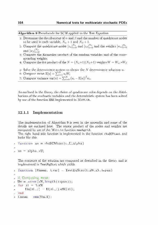
104 Numerical tests for multivariate stochastic PDEs
Algorithm 9 Pseudocode for SCM applied to the Test Equation
1: Determine the distributions of α and β and the number of quadrature nodesto be used in each variable, Nα + 1 and Nβ + 1.
2: Compute the quadrature nodes [zα]Nαi=0 and [zβ ]
Nβi=0 and the weights [wα]Nαi=0
and [wβ ]Nβi=0.
3: Compute the Kronecker product of the random variables and of the corre-sponding weights.
4: Compute the dot product of theN = (Nα+1)(Nβ+1) weightsW = Wα.∗Wβ
5: Solve the deterministic system to obtain the N deterministic solutions u.6: Compute mean E[u] =
∑Ni=1 uiWi
7: Compute variance var(u) =∑Ni=0
(ui − E[u]
)2wi.
As outlined in the theory the choice of quadrature rules depends on the distri-butions of the stochastic variables and the deterministic system has been solvedby use of the function ERK implemented in Matlab.
12.1.1 Implementation
The implementation of Algorithm 9 is seen in the appendix and some of thedetails are outlined here. The tensor product of the nodes and weights arecomputed by use of the Matlab function meshgrid.The right hand side function is implemented in the function rhsSCMtest andlooks like this
1 f unc t i on un = rhsSCMtest ( t ,U, alpha )2
3 un = alpha .∗U;
The statistics of the solution are computed as described in the theory and isimplemented in TestEqStat which yields
1 f unc t i on [Umean , Uvar ] = TestEqStat (U,zW, zN , tspan )2
3 % Computing mean :4 Um = zero s (zN , l ength ( tspan ) ) ;5 f o r z i = 1 : zN6 Um( zi , : ) = U( z i , : ) ∗zW( z i ) ;7 end8 Umean = sum(Um, 1 ) ;

12.1 Test Equation with two random variables 105
9
10 % Computing var iance :11 Uv=ze ro s ( l ength ( tspan ) ,zN) ;12 f o r z i = 1 : zN13 Uv( : , z i ) = (U( z i , : )−Umean( end , : ) ) .^2∗zW( z i ) ;14 end15 Uvar = sum(Uv, 2 ) ; Uvar = Uvar ' ;
The computation of the exact mean and variance have been outlined in thetheory and the implementation TestEqEx can be seen in appendix B.
12.1.2 Gaussian distributed α-parameter and initial con-
dition β
The multivariate Test equation is solved for the case where α and β are bothGaussian distributed. The α-parameter is chosen to be standard normal dis-tributed, i.e. α ∼ N (0, 1), and the initial condition is distributed as β ∼ N (1, 1).Due to the distribution of the stochastic parameters the Gauss Hermite quadra-ture is chosen and six points are chosen in each dimension which leads to 36deterministic solutions due to the tensor product of the grid points.In gure 12.1 the 36 deterministic solutions are plotted.
0 0.5 1
−50
0
50
100
t
Solutions
Figure 12.1: The N = 36 deterministic solutions.
It is seen that there is big variations in the 36 solutions. A dierence from theunivariate case is that now there are negative solutions which was not obtainedpreviously and this means that a single deterministic solution can dier a lotfrom the computed mean since it could be dierent in sign and very dierentin size. The negative solutions are obtained since some of the computed initial

106 Numerical tests for multivariate stochastic PDEs
conditions are negative which leads to negative solutions.The 36 deterministic solutions have been used to compute the statistics. Theestimated mean u can be seen in gure 12.2 with an error bound computed byu± σ as well as the exact mean.
0 0.5 1
−2
0
2
4
t
Mean
StdMeanµ
Figure 12.2: The estimated mean with the computed standard deviation andthe exact mean.
From gure 12.2 it is seen that the mean has not changed a lot in comparisonwith the mean in gure 7.8.In gure 12.2 it is seen that the stochastic initial condition introduces a lot moreuncertainty in the solution in the rst half of the time domain compared to 7.8.With time the eects of the stochastic initial condition becomes less dominantsince the variance introduced by the α-parameter increases exponential withtime.The errors in mean and variance have been computed for dierent M and ingure 12.3 the errors have been plotted as function of M , where mα = mβ = mwhich means that M = m2.

12.1 Test Equation with two random variables 107
100 101 102 103 104
10−10
10−6
10−2
M
Error
MeanVariance
Figure 12.3: Error on the mean and variance for increasing M at time t = 1.
From the errors in gure 12.3 it is seen that the errors converge like it did inthe univariate case except that now it is a function of M instead of just m1.Unless the stochastic β reduces the eects of the stochastic α it is expectedthat at least M = 81 is needed for achieving the smallest error in the meansince M = m2 and mα = 9 was needed to minimize the error in α. ApparentlyM = m2 = 81 is the optimal choice with regard to the error in the mean. Thisindicates that either is the eects of the parameter α reduced or else it holdsthat the best approximation in the mean can be obtained with mβ ≤ mα.A simple test of this assumption is to maintain mα = 2 while increasing mβ andvice versa. This results in the error-plots in gure 12.4.
101 102
10−1
100
M
Error
mβ = 2
101 102
10−10
10−5
100
M
Error
mα = 2
MeanVariance
Figure 12.4: Error on the mean and variance at time t = 1 for increasing M .Left: mβ = 2 and increasing mα. Right: mα = 2 and increasingmβ .

108 Numerical tests for multivariate stochastic PDEs
From the two plots it is seen that it is the number of quadrature points forrepresenting α that makes a dierence with regard to the convergence of the es-timated mean and variance. The number of quadrature points used to representthe β-parameter does not have a great impact on the quality of the estimates.This means that instead of using M = 9 · 9 = 81 deterministic solutions it issucient to compute M = 9 · 2 = 18 deterministic solutions as long as mα = 9and mβ = 2 and not the other way around.This means that the α-parameter has much more inuence on accuracy of theapproximations of the statistics than the β-parameter. This is a good exampleon how a smart choice of quadrature nodes in each stochastic dimension canlead to much more ecient computations without compromising the quality ofthe approximations.
12.1.3 Gaussian distributed α and uniformly distributed
initial condition β.
In this section it has been investigated how it aects the statistics of the solutionto have two stochastic variables with dierent distributions namely α ∼ N (0, 1)and β ∼ U(0, 2). Since β is uniformly distributed the quadrature chosen for thisvariable is Gauss Legendre quadrature. There are again 6 quadrature nodes andweights for both α and β which by use of tensor product leads to 36 deterministicsolutions. Like in the previous test case the deterministic solutions are plottedand can be seen in gure 12.5.
0 0.2 0.4 0.6 0.8 1
0
20
40
t
Solutions
Figure 12.5: 12 of the N = 36 deterministic solutions.

12.1 Test Equation with two random variables 109
The deterministic solutions in gure 12.5 are dierent from the ones in gure12.1 since none of them are negative and they do not grow as much as whenβ was Gaussian distributed. This is because the quadrature nodes are strictlylimited to be in the interval [0, 2] in contrast to the other test case where β wasnot limited in this way.A comparison of the deterministic solutions in gure 12.5 with the ones ingure 12.1 yields that it can have a great impact on the individual deterministicsolution whether β is Gaussian or uniformly distributed. This dierence ishowever not so visible when looking at the statistics as illustrated in gure 12.6where the estimated mean, the std-bound and the exact mean are plotted.
0 0.2 0.4 0.6 0.8 1
0
2
4
t
StdMeanµ
Figure 12.6: The estimated mean with the computed standard deviation aswell as the exact mean.
It is seen that the mean is not greatly aected by the distribution of β butthe standard deviation is dierent than the one seen in gure 12.2. It is smallerwhen β is uniformly distributed than when β is Gaussian distributed. Especiallyin the rst half of the time domain the dierence in the standard deviation isvisible.For this choice of parameters the error has been plotted in gure 12.7 as functionof M = m2 where m = mα = mβ .

110 Numerical tests for multivariate stochastic PDEs
100 101 102 103 104
10−10
10−6
10−2
M
Error
MeanVariance
Figure 12.7: Error on the mean and variance for increasing M at time t = 1.
The tendency in the error in gure 12.7 is the same as was seen in gure 12.3.Again the optimal choice seems to be M = 81 which could indicate that theerror is not greatly aected by the choice of distribution of β. But it worthto remember that the β-parameter apparently has much less inuence on theaccuracy than the α-parameter which means that with 9 quadrature points torepresent β the shift in distribution should not change a lot.To investigate this further the same simple test as was conducted in the previoussection is conducted here. This means that mα = 2 is maintained while mβ isincreased and vice versa. This resulted in the error-plots visualized in gure12.8.
101 102
10−1
100
M
Error
mβ = 2
101 102
10−10
10−5
100
M
Error
mα = 2
MeanVariance
Figure 12.8: Error on the mean and variance at time t = 1 for increasing M .Left: mβ = 2 and increasing mα. Right: mα = 2 and increasingmβ .

12.2 Multivariate Burgers' Equation 111
From the error plots it seems that the α-parameter is still the most dominantparameter when computing the statistics of the multivariate Test equation.Furthermore the change in distribution of β does not seem to have changed theoptimal number of quadrature points to represent α and β which means thatmα = 9 and mβ = 2, and 18 deterministic solutions are sucient to obtain areasonable approximations of the mean.
12.2 Multivariate Burgers' Equation
In this chapter it will be investigated how the statistics of the stochastic Burgers'equation will be aected by introducing uncertainty in both boundary conditionand in the ν-parameter. The uncertainty in the BC's will be assumed to beuniformly distributed and therefore Gauss Legendre quadrature will be used tocompute the quadrature nodes.
12.2.1 Burgers' Equation with stochastic boundary con-
ditions
The 2-variate stochastic Burgers' equation is solved in this section and the eectsof having stochastic BC's are investigated. First the outline of how the SCM isused on the multivariate Burgers' equation is outlined in Algorithm 10.
Algorithm 10 Pseudocode for SCM applied to the 2-variate stochastic Burgers'equation
1: Compute the spatial collocation points x.2: Compute the dierential matrices D and D2.3: Compute the quadrature nodes zb1 and zb2 and the corresponding weightswb1 and wb2 .
4: Compute the tensor product of the weights and nodes to obtain Zb1 , Zb2and W.
5: Compute the initial condition IC.6: Use a deterministic solver to solve the system in time (reach steady state).
7: Compute the mean E[u] =∑Mi=0 uiWi
8: Compute the variance var(u) =∑Mi=0
(ui − E[u]
)2Wi.
In general the approach is very similar to the approach used for the univariateBurgers' equation. The main dierence is the computation of the stochastic

112 Numerical tests for multivariate stochastic PDEs
grids and weights as well as the initial condition. Therefore the implementationof this is outlined in section 12.2.1.1.
12.2.1.1 Implementation
In this section the implementations that are signicantly dierent than the im-plementations in univariate case is outlined. The rest of the code can be foundin appendix B.The interesting part is implemented in theMatlab function InitBurg2D whichlooks like this
1 f unc t i on [ InitCond ,U, Z ,ZW] = InitBurg2D (zN , alpha , beta , nu ,x , dStart , dEnd)
2
3 ck=0; xL = length (x ) ;4
5 Uexact = @(x , t , nu ) −tanh ( ( x−t ) /(2∗nu) )+ck ;6
7 [ z1 ,z1W] = JacobiGQ( alpha , beta , zN−1) ;8 [ z2 ,z2W] = JacobiGQ( alpha , beta , zN−1) ;9
10 % Sca l i ng the weights11 z1W = z1W/2 ;12 z2W = z2W/2 ;13
14 % Sca l i ng the d i s tu rbance s .15 z1 = ( ( z1+1)/2) ∗(dEnd(1)−dStart (1 ) )+dStart (1 ) ;16 z2 = ( ( z2+1)/2) ∗(dEnd(2)−dStart (2 ) )+dStart (2 ) ;17
18 [ Z1 , Z2 ] = ndgrid ( z1 , z2 ) ;19 [Z1W,Z2W] = ndgrid (z1W,z2W) ;20
21 Z1 = Z1 ( : ) ; Z2 = Z2 ( : ) ;22 Z = [ Z1 Z2 ] ;23
24 Z1W = Z1W( : ) ; Z2W = Z2W( : ) ;25 ZW = Z1W.∗Z2W;26
27 % I n i t i a l i z a t i o n and pre−a l l o c a t i o n .28 de l ta1 = Z1 ;29 de l ta2 = Z2 ;30 ZN = length (Z1) ;31 InitCond = Uexact (x , 0 , nu ) ;

12.2 Multivariate Burgers' Equation 113
32 U = zero s (xL∗ZN, 1 ) ;33
34 f o r i = 1 :ZN35 InitTemp = InitCond ;36 InitTemp ( InitTemp>0) = InitTemp ( InitTemp>0)∗(1+ de l ta1
( i ) ) ;37 InitTemp ( InitTemp<0) = InitTemp ( InitTemp<0)∗(1+ de l ta2
( i ) ) ;38 U(xL∗( i −1)+1:xL∗( i ) ) = InitTemp ;39 end
The BC's are uniformly distributed which means that Gauss Legendre quadra-ture is used.The function ndgrid is used to compute all combinations of the nodes and ofthe weights. Then the weights are multiplied to attain the tensor product.The initial condition is computed by using the exact solution and then changethe values that are higher or lower than zero according to the grid of stochasticBC's. This is not strictly necessary in order to obtain good results but it speedsup the iteration process.
12.2.1.2 Tests
In this test a space grid of 31 points have been used and boundary conditionsare distributed with u(−1) ∼ U(1, 1.1) and u(1) ∼ U(−1,−1.1).The tests have been conducted with 4 quadrature points in each stochastic di-mension which means that 16 deterministic solutions have been computed.The one dimensional dierentiation matrix D and its square D2 are of dimen-sion 31×31 which means that the dierentiation matrix for all the deterministicsolutions is a (18 ·31)× (18 ·31) matrix. In this matrix 1
18 'th of the elements arenon-zero which means that the sparse structure of the matrix is denitely worthto utilize. If there had been used more quadrature points the system would havebeen even more sparse which is worth to note when solving the deterministicsystem.The 18 deterministic solutions are plotted in gure 12.9 and have some inter-esting characteristics.

114 Numerical tests for multivariate stochastic PDEs
−1 −0.5 0 0.5 1
−1
0
1
x
Solutions
Figure 12.9: The M = 18 deterministic solutions for Burgers' Equation.
From gure 12.9 it is seen that the deterministic solutions are characterizedby three dierent behaviours. The rst kind of deterministic solutions are theones recognized from the previous univariate test case where the transition layeris shifted to the far right in the plot due to a positive disturbance in the leftboundary. This was the tendency that was observed in the univariate case andit is not surprisingly also present in this multivariate test since some of thedeterministic solutions are characterized by disturbances in the left boundarybut (almost) none in the right boundary.The second type of deterministic solutions are when there are disturbances inboth BC's and the transition layer is located in at x = 0. This means thatsome of the deterministic solutions have the same characteristics in terms ofthe transition layer as the unperturbed deterministic solution but with shiftedboundary values such the values in u(−1) are a bit higher than the originaldeterministic solution and the values in u(1) are a bit lower.The last kind of deterministic solutions are the opposite of what was observed inthe univariate test case, namely that there is disturbance in the right boundaryand (almost) none in the left boundary which means that the transition layer isshifted to the far left.The multivariate Burgers' equation yields deterministic solutions that are muchdierent from the ones obtained in the univariate case since some of the solutionsare very similar to the unperturbed deterministic solution and since there issolutions where the transition layer is shifted both to the left and to the right.The statistics of the multivariate Burgers' equation have also been computedand in gure 12.10 the mean and variance can be seen.

12.2 Multivariate Burgers' Equation 115
−1 −0.5 0 0.5 1
−1
0
1
x
Mean
±stdVarMeanBound
Figure 12.10: The estimated mean and variance and bounds on the solutions.
In gure 12.10 it is seen that the behaviour of the mean is very dierent fromthe mean computed for the univariate Burgers' equation and the solution of thedeterministic Burgers' equation. Instead of having one transition layer wherethe mean goes from 1 to −1 it is divided into three.It is also seen that there is a large variance and the uncertainty of this solutionsis greater than seen for the other test cases.
12.2.2 3-variate Burgers' equation
Now the ν-parameter is chosen to be stochastic as well as the BC's. Thismeans that it is now a three dimensional stochastic system and due to thetensor product of the stochastic variables this results in a potentially very largesystem. The overall approach is very similar to the 2-variate case and is outlinedin Algorithm 11.

116 Numerical tests for multivariate stochastic PDEs
Algorithm 11 Pseudocode for SCM applied to the 3-variate stochastic Burgers'Equation
1: Compute the spatial collocation points x.2: Compute the dierential matrices D and D2.3: Compute the quadrature nodes zb1 , zb2 and zν and the corresponding weightswb1 , wb2 and wν .
4: Compute the tensor product of the weights and nodes to obtain Zb1 , Zb2 ,Zν and W.
5: Compute the initial condition IC.6: Use a deterministic solver to solve the system in time (reach steady state).
7: Compute the mean E[u] =∑Mi=0 uiWi
8: Compute the variance var(u) =∑Mi=0
(ui − E[u]
)2Wi.
By comparison of the pseudocodes in algorithm 10 and 11 it is seen that mostof the steps are the same and some of the implementations can be reused. Inthe tests presented here the BC's are again chosen to be uniformly distributedas well as the ν-parameter.The ν-parameter is very interesting since it is the viscosity of the Burger's equa-tion and determines the smoothness of the PDE. If ν = 0 there would be a shockdiscontinuity instead of a transition layer [19].The polynomial representations used in the spectral methods are not well suitedfor describing discontinuities and ν = 0 would therefore pose a serious problem.During the numerical tests a small ν was chosen which could not be solved withthe current settings. This problem might be dealt with by using some otherrepresentations than the orthogonal polynomials but it is outside the scope ofthis thesis to investigate that.If the ν-parameter is increased the solution of Burgers' equation becomes smootherand the transition layer would not be a region of such rapid change. It would inother words result in a very dierent solution which will be seen in the numericalexperiments.
12.2.2.1 Implementation
The interesting part of the implementations compared to the earlier implemen-tations is where the quadratures are used and the initial condition is computed.This is done in the Matlab function InitBurg3D that is included here whilethe rest of the implementation is in appendix B.
1 f unc t i on [ InitCond ,U, Z ,ZW] = InitBurg3D (zN , alpha , beta , nu ,x , dStart , dEnd)

12.2 Multivariate Burgers' Equation 117
2
3 ck=0; xL = length (x ) ;4
5 Uexact = @(x , t , nu ) −tanh ( ( x−t ) /(2∗nu) )+ck ;6
7 % Computing the quadrature weights and nodes f o r therandom BC' s
8 [ z1 ,z1W] = legendrequad (zN) ;9 [ z2 ,z2W] = legendrequad (zN) ;
10
11 % Sca l i ng the weights12 z1W = z1W/2 ;13 z2W = z2W/2 ;14
15 % Sca l i ng the d i s tu rbance s .16 z1 = ( ( z1+1)/2) ∗(dEnd(1)−dStart (1 ) )+dStart (1 ) ;17 z2 = ( ( z2+1)/2) ∗(dEnd(2)−dStart (2 ) )+dStart (2 ) ;18
19 % Computing the nodes and weights f o r the nu paremeter20 i f strcmp (nu . t , ' uniform ' )21 [ z3 ,z3W] = JacobiGQ( alpha , beta , zN−1) ;22
23 % Sca l i ng the weights and nu24 z3W = z3W/2 ;25 z3 = ( ( z3+1)/2) ∗(nu . par (2 )−nu . par (1 ) )+nu . par (1 ) ;26
27 e l s e i f strcmp (nu . t , ' normal ' )28 [ z3 ,z3W] = HermiteQuadN(zN) ;29
30 % Sca l i ng nu31 z3 = nu . par (1 )+nu . par (2 ) ∗ z3 ;32 end33 %z3 = 0 . 0 5 ; z3W = 1 ;34 [ Z1 , Z2 , Z3 ] = ndgrid ( z1 , z2 , z3 ) ;35 [Z1W,Z2W,Z3W] = ndgrid (z1W,z2W,z3W) ;36
37 Z1 = Z1 ( : ) ; Z2 = Z2 ( : ) ; Z3 = Z3 ( : ) ;38 Z = [ Z1 Z2 Z3 ] ;39
40 Z1W = Z1W( : ) ; Z2W = Z2W( : ) ; Z3W = Z3W( : ) ;41 ZW = Z1W.∗Z2W.∗Z3W;42
43 % I n i t i a l i z a t i o n and pre−a l l o c a t i o n .44 de l ta1 = Z1 ; de l t a2 = Z2 ; ZN = length (Z1 ) ;

118 Numerical tests for multivariate stochastic PDEs
45 nuEst = sum( z3 ) /zN ;46 InitCond = Uexact (x , 0 , nuEst ) ;47 U = zero s (xL∗ZN, 1 ) ;48
49 f o r i = 1 :ZN50 InitTemp = InitCond ;51 InitTemp ( InitTemp>0) = InitTemp ( InitTemp>0)∗(1+ de l ta1
( i ) ) ;52 InitTemp ( InitTemp<0) = InitTemp ( InitTemp<0)∗(1+ de l ta2
( i ) ) ;53 U(xL∗( i −1)+1:xL∗( i ) ) = InitTemp ;54 end
The implementation is very similar to the code used in the two dimensional caseand the interesting part is the computation of the tensor grids.It might seem like an innocent extension of the code used previously but it leadsto a very increased computational eort. This is due to the fact that M = m3
if mBC1 = mBC2 = mν = m which means that the dierentiation matrices areincreased very much in size which makes the deterministic system much morecostly to solve.
In the tests there are used 61 space points and m = 4 for each stochas-tic dimension which means that the dierentiation matrices are of the size(61 · 43) × (61 · 43) = 3904 × 3904. This means that the two matrices con-tains 15,241,216 elements. Only a fraction of 1
64 of these elements are non-zerowhich is about 1.5 % but it is still a large system that potentially has to besolved many times - depending on the solver - in order to reach steady state.Assuming that m = 5 quadrature points are needed in each dimension to obtainthe desired accuracy it will result in a much larger to system. Instead of hav-ing 64 deterministic solutions there is now 125 and the dierentiation matricesare now of the size (61 · 53) × (61 · 53) = 7625 × 7625 and contains 58,140,625elements. Even though "only" 465,125 elements are non-zero it is still a largesystem and it shows how important it is not to use too many quadrature pointsif it is not needed. It also demonstrates that when the dimensionality of a prob-lem is increased the computational eort can be increased very much.
This example is a three dimensional stochastic problem and many of the stochas-tic PDE's to be solved have 50 or 100 which illustrates that the growth in thecomputational eort is a real problem in practise.It is clear that sparsity has to be utilized when it is possible - both when solvingthe deterministic system but also - if possible - when computing the quadrature
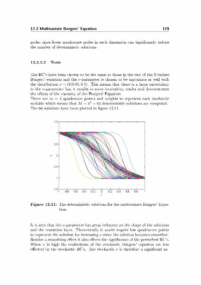
12.2 Multivariate Burgers' Equation 119
nodes since fewer quadrature nodes in each dimension can signicantly reducethe number of deterministic solutions.
12.2.2.2 Tests
The BC's have been chosen to be the same as those in the test of the 2-variateBurgers' equation and the ν-parameter is chosen to be univariate as well withthe distribution ν ∼ U(0.05, 0.5). This means that there is a large uncertaintyin the ν-parameter but it results in some interesting results and demonstratesthe eects of the viscosity of the Burgers' Equation.There are m = 4 quadrature points and weights to represent each stochasticvariable which means that M = 43 = 64 deterministic solutions are computed.The 64 solutions have been plotted in gure 12.11.
Figure 12.11: The deterministic solutions for the multivariate Burgers' Equa-tion.
It is seen that the ν-parameter has great inuence on the shape of the solutionsand the transition layer. Theoretically it would require less quadrature pointsto represent the solution for increasing ν since the solution becomes smoother.Besides a smoothing eect it also eects the signicance of the perturbed BC's.When ν is high the realizations of the stochastic Burgers' equation are lesseected by the stochastic BC's. The stochastic ν is therefore a signicant pa-

120 Numerical tests for multivariate stochastic PDEs
rameter when conducting UQ for Burgers' equation.The eect on the statistics of having three stochastic variables have also beeninvestigated. In gure 12.12 the mean and variance are plotted.
−1 −0.5 0 0.5 1
−1
−0.5
0
0.5
1
x
Mean
±stdVarMean
Figure 12.12: The mean, variance and bounds by standard deviation for thecomputed solution.
It is seen that the variance is relatively small compared to the one obtained inthe 2-variate case and the transition layer in the mean is much smoother thanpreviously which means that the stochastic ν-parameter has a smoothing eecton the mean and dampens the variance.It seems like the stochastic ν-parameter decreases the variance of the solutionbut as seen from gure 12.11 there are larger variations in the deterministicsolutions. Hence the smaller variance is not a result of very similar solutionsbut of the fact that the steep solutions have less inuence on the statistics thanthe smooth solutions.It is worth to note that the transition layer of the estimated mean is centredaround x = 0 as it is for the unperturbed solution. The transition layer inthe estimated mean does not give an exact representation of the solution tothe unperturbed problem but it gives a better impression of the location ofthe transition layer than e.g. the estimated mean for the univariate Burgers'equation.

12.2 Multivariate Burgers' Equation 121
12.2.2.3 Test with a dierent right BC
In this section the right BC have been changed such that it is distributed asu(1) ∼ U(−0.9,−1). The rest of the settings are the same as before and m = 4for each stochastic variable which implies that 64 deterministic solutions havebeen computed. These solutions have been plotted in gure 12.13.
Figure 12.13: The deterministic solutions for the multivariate Burgers' Equa-tion.
In gure 12.13 it seen that that there are no deterministic solutions which havea transition layer shifted to the left and that there are more solutions which areshifted to the right than previously. This will naturally aect the statistics asseen in gure 12.14 where the estimated mean and variance are plotted.
−1 −0.5 0 0.5 1
−1
0
1
x
Mean
±stdVarMean
Figure 12.14: The estimated mean and variance.

122 Numerical tests for multivariate stochastic PDEs
The estimated mean and variance are skewed to the right in gure 12.14 com-pared to the results plotted in gure 12.12 and the transition layer is steeper.
Based on the investigations of the multivariate problems it safe to say that thestochastic parameters have a great inuence on the solutions of the problems.Furthermore the eects of a stochastic parameter might be lessened or increasedif another stochastic parameter in introduced and UQ is denitely a useful toolwhen working with e.g. stochastic PDEs. But as outlined in this chapter thereare some diculties that need to be solved and one of the main problems isthe growth in computational eort when the number of stochastic variables isincreased.

Chapter 13
Tests with Smolyak sparsegrids
From the theory outlined previously it follows that each collocation node impliesto compute a deterministic solution to the system at hand. This means that thesparse grids potentially implies a signicantly reduction in the computationalwork and it is therefore lucrative to use sparse grids instead of the full tensorgrids.It is furthermore to be noted that the use of sparse grids becomes increasinglybenecial for increasing dimensions. The decreased computational eort andtime consumption motivates the use of the sparse grids even though it shouldbe noted that the sparse grids are not a cure to the curse of dimensionality butonly a remedy to ensure a lessened impact.
The implementations made by John Burkardt [2] are used to conduct tests withthe sparse Gauss Legendre (SGL) grid and the sparse Clenshaw-Curtis (CC)grid.Both types of sparse grids are often used to represent uniformly distributedstochastic variables. The relationship between the grids and the distribution ofthe variables is similar to the relationship between the orthogonal polynomialsand the distributions outlined in Table 4.1. This means that the two types ofgrids should be optimal when used to represent uniformly distributed variables

124 Tests with Smolyak sparse grids
but they can be used for stochastic variables with other distributions.It should be noted that the Smolyak grids in general are not restricted to repre-sent uniformly distributed variables and there are many types of Smolyak sparsegrids that can be applied.
13.1 Introduction of the sparse grids
The two sparse grids will be introduced further in this section and in the follow-ing sections they will be used to estimate the statistics of the stochastic solutionsof the Test equation and the stochastic Burgers' equation.
13.1.1 Sparse Gauss Legendre grid
The sparse Gauss Legendre (SGL) grid is based on 1D Gauss Legendre quadra-ture rules which are combined, as introduced in section 11.3.According to [2] the total number of nodes M in the sparse Gauss Legendregrid is coupled to the level and the stochastic dimension d as illustrated in table13.1.
Level / d 1 2 30 1 1 11 3 5 72 9 21 373 23 73 1594 53 225 5975 115 637 20316 241 1693 6405
Table 13.1: Total number of points in the sparse Gauss Legendre grid.
The level here refers to the maximum attained level in the sparse grid which isrepresented by N in (11.4) and (11.5).It should be noted that according to [2] the sparse Gauss Legendre grid is weaklynested in the sense that all the odd levels contain the value X = 0.0.This is reected in the outcome of the implementations since this point is re-peated once for each odd level and once for level 0. This means that the two-dimensional SGL grid with level 2 contains 22 points where 21 are unique andwith level l = 3 there are 75 points in the returned grid and 73 of these areunique. The grid points for level l = 2 which contains 21 unique points is plot-

13.2 Sparse Clenshaw-Curtis grid 125
ted in gure 13.1. The SGL grid has been plotted as well as a full tensor gridbased on Gauss Legendre quadrature with 7 nodes in each stochastic dimension.The numerical tests for the Test equation includes a comparison of the accuracyof the estimates based on these two grids.
−1 0 1
0
1
2
Z1
Z1
Full grid
−1 0 1
−1
0
1
Z1
Z1
SGL grid
Figure 13.1: Left: A full tensor grid with 7 Gauss Legendre quadrature pointsin each dimension. Left: The SGL grid with level l = 2 and 21unique nodes.
13.2 Sparse Clenshaw-Curtis grid
A major dierence between the Clenshaw-Curtis (CC) grid and the SGL grid isthat the Clenshaw-Curtis grid is nested. This means that the grid at a certainlevel is contained in a grid of a higher level. Another important dierence be-tween the two types of grids is that CC contains nodes on the boundary wherethe SGL only contains interior points. This can make a big dierence can beseen in the numerical tests for Burgers' equation.The CC grids does not follow the same correspondence between total number ofnodes in the grid and the level l and dimension d, as was introduced in Table 13.1.In [4] this relationship is outlined for the CC grid and it can be seen in Table 13.2.

126 Tests with Smolyak sparse grids
level / d 1 2 30 1 1 11 3 5 72 5 13 253 9 29 694 17 65 1775 33 145 441
Table 13.2: Total number of nodes in the sparse Clenshaw-Curtis grid.
It is seen that for the same level the CC grid contains fewer points than the SGLgrid. But the SGL grid has higher accuracy if the same level is applied. Theaccuracy of the two grids for specic levels will be investigated in the numericaltests for the Test equation.It should be noted that the higher the dimension the larger is the dierence inthe number of points. This means that even though the SGL grid should bemore ecient than CC for a certain level, the CC grid might be worth to use inhigh dimensions since the computational eort is much smaller.
A plot of the 65 grid points for a level 4 sparse CC grid is plotted in gure 13.2as well as a full tensor grid of 17 points in each dimension.
−1 0 1
−1
0
1
Z1
Z1
Full grid
−1 0 1
−1
0
1
Z1
Z1
CC grid
Figure 13.2: In this gure a full tensor grid is illustrated to left the and to theright a sparse CC grid is plotted.
In gure 13.2 it is seen that the sparse CC grid corresponds to a subset of the fulltensor grid. The application of the sparse CC grid can be seen in the followingsections.

13.3 Smolyak sparse grid applied 127
13.3 Smolyak sparse grid applied
In this section the results of the numerical tests with the two sparse grids arepresented. The numerical tests involve the 2-variate Test equation and the 2-variate Burgers' equation.The implementations for this section are very similar to the ones used in theprevious multivariate tests with the only dierence that the tensor grids ofquadrature points have been replaced with the sparse grids. This means that therhs-function, the deterministic solver etc. are the same as previously. Becauseof this the implementations have not been included here but the test scripts canbe found in appendix B. For the implementations of the sparse grid the readeris referred to [2].
13.3.1 The 2-variate Test Equation
The stochastic Test equation with uniform α and β has been investigated usingthe two sparse grids. The two variables are distributed with α ∼ U(−1, 1) andβ ∼ U(0, 2).The SGL grid and CC grid with level 3 have been used to estimate the statisticsfor the stochastic Test equation and the results can be seen in the followingsections. Since the estimates of the statistics are very similar to the ones ob-tained with the full tensor grids the numerical tests in this section will be aninvestigation of the errors. Furthermore the accuracy of the the grids havebeen compared with the accuracy obtained with the full tensor grid in section13.3.1.3.
13.3.1.1 Sparse Gauss Legendre grid
In this section the SGL grid is applied and the error of the obtained estimateshave been computed. The errors have been plotted as functions of the totalnumber of grid points, M . The correspondence between number of points andthe levels can be seen in table 13.1. The grids have been computed for the levelsl = 0, 1, . . . , 6 and the errors for the corresponding grid sizes have been plottedin gure 13.3.

128 Tests with Smolyak sparse grids
100 101 102 10310−13
10−9
10−5
10−1
M
Error
MeanVariance
Figure 13.3: Error of the estimated mean and variance for increasing M attime t = 1.
It is seen that the error drops rather quickly and the error reaches a minimumwhich is equivalent to the minimum error obtained in the previous tests of themultivariate Test equation at level l = 3 where the grid contains 21 uniquepoints.
13.3.1.2 Sparse Clenshaw-Curtis grid
The sparse Clenshaw-Curtis grid has been use to estimate the statistics for themultivariate Test equation. The errors using the CC grid have been plotted ingure 13.4 as function of the total number of grid points, M .

13.3 Smolyak sparse grid applied 129
100 101 10210−13
10−9
10−5
10−1
M
Error
MeanVariance
Figure 13.4: Error of the estimated mean and variance for increasing M attime t = 1.
It is seen that the convergence of the errors when using the CC grid is notimpressive compared to the convergence obtained previously using full tensorgrids. This means that the CC grid might not be suited for estimating thestatistics of this problem.
13.3.1.3 Comparison of the errors on the estimated statistics
As illustrated in gure 13.3 and gure 13.4 the two sparse grids can be usedas collocation points for the stochastic Collocation method which leads to fairresults when the stochastic variables are uniformly distributed. In this sectionthe accuracy of the SCM used with SGL and CC grids is investigated further. Asa comparison the SCM has been used with full tensor grid on the same problemand the errors are included in Table 13.3.The full tensor grids are computed from 1D Gauss Legendre quadrature andthe same number of quadrature nodes has been used in each dimension, i.e.the total number of nodes is M = m1 × m2 = m2 where m is the number ofquadrature nodes in each dimension.

130 Tests with Smolyak sparse grids
M Error in the mean Error in the variance1 1.75 · 10−1 1.044 3.85 · 10−3 8.34 · 10−2
9 3.28 · 10−5 2.98 · 10−3
16 1.48 · 10−6 5.39 · 10−5
25 4.13 · 10−10 5.98 · 10−7
36 1.63 · 10−12 4.52 · 10−9
49 8.43 · 10−13 2.91 · 10−10
64 8.41 · 10−13 4.50 · 10−12
81 8.42 · 10−13 4.49 · 10−12
100 8.41 · 10−13 4.49 · 10−12
Table 13.3: The errors in the estimated statistics and the corresponding num-ber of nodes in the full tensor grid.
From table 13.3 it is seen that the minimum error in the mean is obtained for49 grid points and 64 grid points for the variance. This corresponds very wellwith the investigations made previously for the univariate Test equation withuniformly distributed α. In this case 7 quadrature nodes was needed to obtainthe minimum error in the estimated mean and 8 quadrature nodes to obtain theminimum error in the estimated variance.Furthermore the previous numerical tests with the 2-variate stochastic Testequation indicated that the α-parameter was more dominant than β in termsof the error in the estimated statistics. This corresponds very well with theoptimal number of tensor grid points for the full tensor grid since it correspondsto chose the optimal choice of quadrature nodes for α in each dimension.
The SGL grid is used as collocation points for the SCM for the stochastic Testequation. The grids with level l = 0, 1, . . . , 6 are used and the errors of theestimated statistics are outlined in table 13.4. A comparison of Table 13.4eciency of the SCM is higher when using the SGL grids than when using fulltensor grids in the sense that the same accuracy is obtained using SGL gridsbut with fewer grid points.

13.3 Smolyak sparse grid applied 131
Level M Error in the mean Error in the variance0 1 1.75 · 10−1 1.0371 5 3.27 · 10−5 2.73 · 10−1
2 22 8.42 · 10−13 7.65 · 10−4
3 75 8.42 · 10−13 1.06 · 10−11
4 224 8.40 · 10−13 4.39 · 10−12
5 613 8.40 · 10−13 4.39 · 10−12
6 1578 8.48 · 10−13 4.39 · 10−12
Table 13.4: The errors in the estimated statistics and the corresponding levelsand total number of nodes in the SGL grid.
Numerical tests are conducted using the CC grids as well and this resulted incomputation of the errors of the estimated mean and variance which can be seenin Table 13.5.
Level M Error in the mean Error in the variance0 1 1.75 · 10−1 1.041 5 5.83 · 10−3 1.78 · 10−1
2 13 1.35 · 10−5 3.49 · 10−2
3 29 1.11 · 10−11 3.06 · 10−4
4 65 8.39 · 10−13 3.81 · 10−9
5 145 8.39 · 10−13 4.39 · 10−12
6 321 8.40 · 10−13 4.39 · 10−12
Table 13.5: The errors of the estimated statistics and the corresponding levelsand number of nodes in the CC grid.
The accuracy of the CC grids is lower than the accuracy obtained using the SGLgrids on this particular test problem. This is not necessarily true in general butit still yields an interesting result. It seems like fewer grid points are neededwhen using the full tensor grid than when using the CC grid to obtain theminimum error. But this is might just be due to the fact that the CC grid has29 grid points in the level 3 grid and 65 grid points for level 4. This means thatbecause the optimal choice of level is not level 3 at least 65 nodes are used toobtain the best estimates which is more than in the full grid.It is furthermore to be noted that the CC grid might be much more useful inhigher dimensions than 2 since the sparse grids are introduced to reduce theeects of the curse of dimensionality in high dimensions.

132 Tests with Smolyak sparse grids
13.3.1.4 Discussion
The sparse grids seems to be very useful and the use of the SGL grid denitelydemonstrates that a high accuracy can be obtained with fewer nodes in com-parison to the full tensor grid.It should be noted that for the stochastic Test equation it seems like α is moredominant in terms of inuence on the error than β. Therefore a full tensorgrid might involve fewer quadrature nodes to represent β and thereby lead toa smaller number of total nodes, while maintaining a high accuracy. Thereforethe sparse grids are more ecient than the full tensor grids investigated in thissection but smarter grids might be applied which are full tensor grids but stillinvolves relatively few grid points.This is one of the reasons why a method like ANOVA can be very useful sinceANOVA can be used to investigate which of the stochastic variables that havea great inuence on the statistics and which of them are less important.
13.3.2 The 2-variate Burgers' Equation
The SCM is tested for the stochastic Burger' equation using the two Smolyaksparse grids introduced previously. The tests are conducted for the case wherethe BC's are stochastic and distributed as u(−1, t) ∼ U(1, 1.1) and u(1, t) ∼U(−1,−0.9).
13.3.2.1 Sparse Gauss Legendre grid
In this section SGL is used as collacation points when computing estimates ofthe statistics for the Burgers' equation with stochastic BCs.The SGL grid with level l = 2 and a total of 21 unique nodes results in theestimates of the statistics plotted in gure 13.5.
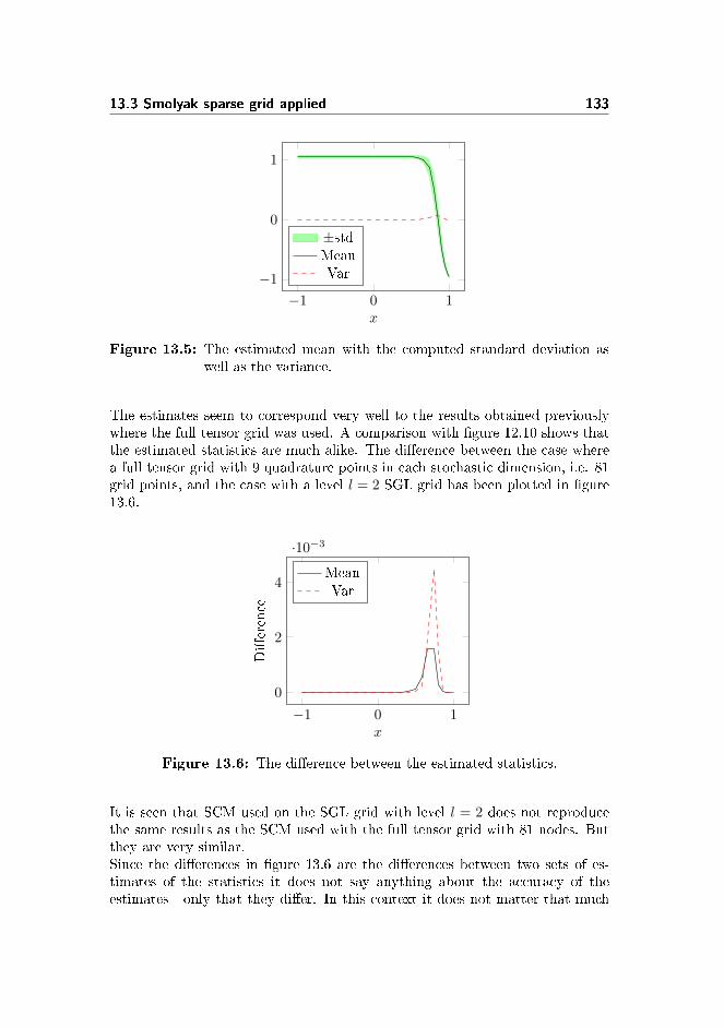
13.3 Smolyak sparse grid applied 133
−1 0 1
−1
0
1
x
±stdMeanVar
Figure 13.5: The estimated mean with the computed standard deviation aswell as the variance.
The estimates seem to correspond very well to the results obtained previouslywhere the full tensor grid was used. A comparison with gure 12.10 shows thatthe estimated statistics are much alike. The dierence between the case wherea full tensor grid with 9 quadrature points in each stochastic dimension, i.e. 81grid points, and the case with a level l = 2 SGL grid has been plotted in gure13.6.
−1 0 1
0
2
4
·10−3
x
Dierence
MeanVar
Figure 13.6: The dierence between the estimated statistics.
It is seen that SCM used on the SGL grid with level l = 2 does not reproducethe same results as the SCM used with the full tensor grid with 81 nodes. Butthey are very similar.Since the dierences in gure 13.6 are the dierences between two sets of es-timates of the statistics it does not say anything about the accuracy of theestimates - only that they dier. In this context it does not matter that much

134 Tests with Smolyak sparse grids
which of the two grids that produces the most accurate estimates since the es-timates are so close and it demonstrates that the sparse grids could be usedinstead of a full tensor grid and it could reduce the computational eort.
13.3.2.2 Sparse Clenshaw-Curtis grid
In this section the CC grid is used as collocation points and the level of theCC grid is chosen to be 2 which means that 13 grid point are used. The 13collocation points implies the computation of 13 deterministic solutions, whichare plotted in gure 13.7.
−1 0 1
−1
0
1
x
Solutions
Figure 13.7: The 13 deterministic solutions for a level 2 CC grid.
It is seen that since the CC grids include boundary points the solution with theunperturbed BC's, i.e. u(−1) = 1 and u(1) = −1, is among the deterministicsolutions. This has not been the case when using the SGL grid and the fulltensor grid and might have a great eect on the estimated statistics - especiallysince the estimates are based on only 13 deterministic solutions.The approximated statistics can be seen in gure 13.8 where it is seen that thestatistics are very dierent from the estimates based on the full tensor grid andthe SGL grid as seen in gure 13.5.

13.4 Conclusion 135
−1 0 1
−1
0
1
x
Statistics
±stdMeanVar
Figure 13.8: The estimated statistics computed by using a CC grid with level2.
It is interesting to see how the estimates have changed due to the inclusion ofthe unperturbed solution and it demonstrates that it can make a great dierencewhich collocation points are used when computing the estimates.This illustrates that the CC grids has some dierent qualities than the SGLgrids and the choice of grid is therefore not only a choice based on accuracy butalso based on the special characteristics of the grids.
13.4 Conclusion
The tests in this chapter have illustrated that the sparse grids can be used toobtain high accuracy results and that they can decrease the number of nodesneeded to obtain these results. Fewer nodes means less deterministic solutionsand thereby less computational eort.The tests with the sparse grids yields some interesting results, but the sparsegrids are designed to be used in high dimensions. This means that the tests of2-variate dierential equations might not illustrate all the benets of using thesparse grids.
As outlined in the beginning of the chapter the two sparse grids have dierentproperties, which has been conrmed in the tests. In order to choose whichsparse grid that is best suited to a given problem the user has to consider bothaccuracy and the properties of the sparse grids.Furthermore the user has to consider whether the use of sparse grids is theoptimal choice of method to reduce the computational eort. Other methodsmight be more ecient in some cases e.g. ANOVA. There are many aspects to

136 Tests with Smolyak sparse grids
consider when handling UQ and the sparse grids is a useful tool that should beconsidered when solving high dimensional problems.

Chapter 14
Discussion
The focus in this thesis has been to investigate spectral methods for UncertaintyQuantication and in particular an investigation of the stochastic Collocationmethod. As a reference the Monte Carlo sampling has been introduced andapplied on the Test equation.The test cases in this thesis has been low dimensional problems which have rel-atively smooth solutions and under these conditions the spectral methods haveproved ecient and accurate.The numerical tests and the outlined theory has denitely motivated the use ofspectral methods which have a much higher convergence rate than the MonteCarlo sampling. But it has also been discovered that the spectral methods hassome weaknesses. One of them is the computational work of especially the Col-location method when applied to problems of higher dimensions. The Galerkinis more ecient than the Collocation method but it comes at the cost of muchmore work in terms of derivations and implementations.Another perspective of the two methods is that the stochastic Galerkin methodusually is based on solving a system of coupled equations whereas the solutionscomputed in the stochastic Collocation method are de-coupled. The de-couplingof the solutions could be utilized by introducing parallel programming. In thisway the computation time could be greatly reduced.
The computational work of the spectral methods can be lessened by use of

138 Discussion
e.g. Smolyak sparse grids. The introduction sparse grids is a useful tool thateven for 2-variate problems can lead to high accuracy and relatively low com-putational eort. In higher dimensions the gain in terms of less computationaleort is even greater. Other methods to achieve the spectral convergence of thespectral methods and decrease the computational eort can be applied like thecompressive sampling method. This means that the spectral methods can bea useful tool not only in low dimensions but potentially in very high dimensions.
The thesis does not include numerical tests in high dimensions and the eciencyof the spectral methods combined with e.g. sparse grids has not been establishedfor high dimensional problems. This means that even though the sparse gridsdecrease the computational eort the Monte Carlo sampling could potentiallystill be more ecient in high dimensions than the spectral methods.Another strength of the Monte Carlo sampling is that the convergence and ac-curacy of the method is independent of the characteristics of the solutions. Thespectral methods introduced in this thesis are based on polynomial representa-tions which means that the solutions should be smooth in order to obtain goodrepresentations. This could pose a considerable problem and for example thesolution of the stochastic Test equation could be dicult to represent by useof spectral methods if the ν-parameter is too low, i.e. the solutions becomenon-smooth.
14.1 Future work
The thesis has focused on one type of method to reduce the eects of the curseof dimensionality which is the use of Smolyak sparse grids. The next step wouldbe to take these investigations further by numerical tests in higher dimensions.These tests could reveal the full potential of the sparse grids and might demon-strate unforeseen qualities or aws of the sparse grids.Another natural step would be to do some numerical tests with the ANOVA,the non-adapted sparse method and the sparse pseudospectral approximationmethod. These tests could be conducted as well as the sparse grid tests inhigh dimensions and a comparison of the accuracy and eciency of the meth-ods could be done. This would be a very comprehensive task if the tests whereto be conducted on several advanced problems in high dimension but it couldreveal some interesting guidelines to when to use which methods.Another interesting perspective could be to utilize that the stochastic Colloca-tion method is based on uncorrelated deterministic solutions by computing thedeterministic solutions by use of parallel programming.Finally it could be interesting to investigate if it is possible to estimate the

14.1 Future work 139
statistics of non-smooth solutions eciently and accurately. Potentially theinvestigations could involve high dimensional problems with non-smooth solu-tions.

140 Discussion

Chapter 15
Conclusion
This thesis introduce and tests three dierent methods for Uncertainty Quan-tication. The Monte Carlo Sampling proved to have slower convergence forthe univariate Test equation but the method is relatively easy to apply and theconvergence is independent of the dimensionality of the problem at hand. Thestochastic Galerkin method and the stochastic Collocation method have greaterconvergence rate for the univariate Test equation but both methods requiresmore computations when the dimensionality is increased.Furthermore it is to be noted that the Monte Carlo sampling is independentof the structure of the solutions - it basicly just requires that enough solutionscan be computed. This is a strength compared to the spectral methods due tothe computational eort in high dimensions for these methods and the fact thatthey are based on approximations with polynomials implies that they can havediculties with representing e.g. non-smooth solutions.The stochastic Galerkin method is in general more accurate than the stochasticCollocation method but requires a lot more work in terms of derivations andimplementation. The stochastic Collocation method is easier to apply but suf-fers under the curse of dimensionality.
Due to the relative ease of use and the spectral convergence the stochastic Col-location method is a popular choice of UQ method. The curse of dimensionalityhas led to a lot of research to minimize the eects. This includes the studies of

142 Conclusion
Smolyak sparse grids and the application of these.The sparse grids can assure high accuracy with a relatively low number of nodeswhich means that the computational eort of the stochastic Collocation methodis greatly reduced since the computational eort of the method is related to thenumber of deterministic solutions which is equal to the number of nodes.
Two dierent types of grids have been used in this thesis and they have dierentcharacteristics. The Clenshaw-Curtis grid is nested and contains the boundarynodes while the sparse Smolyak Gauss Legendre grid is not nested and does notcontain the boundary nodes. The sparse Gauss Legendre grid is more accuratefor a given level than the Clenshaw-Curtisg grid but the Clenshaw-Curtis gridcontains fewer points for each level. This means that in many cases the optimalchoice of sparse grid could be problem dependent.
The Uncertainty Quantication is denitely a useful tool which can be appliedin many dierent settings since uncertainty is present whenever measurementsare made and parameters are estimated. This thesis has introduced spectralmethods for Uncertainty Quantication and tested one method to reduce theeects of the curse of dimensionality but there is without a doubt much morewithin the eld which is worth to study further. Tests in higher dimensionsseems like a natural step from here and the application of other methods aswell could very likely be lucrative. The ANOVA and the compressive samplingdenitely seems like interesting alternatives to the Smolyak grids in order toavoid the eects of the curse of dimensionality.

Appendix A
Supplement to themathematical background
A.1 Orthogonal Polynomials
Here an introduction to an alternative denition of the Hermite Polynomials isgiven.
A.1.1 Alternative denition of the Hermite polynomials
The alternative denition of the Hermite Polynomials is denoted Hn(x) and isbased on the following weight functions
wH(x) =1√πe−x
2
Furthermore the denition of Hn(x) is
Hn(x) =1
(−1)ne−x2
dn
dxn[e−x
2
] = n!
[n/2]∑k=0
(−1)k1
k!(n− 2k)!(2x)n−2k.

144 Supplement to the mathematical background
The three-term recurrence relation is
Hn+1(x) = 2xHn(x)− 2nHn−1(x), (A.1)
with H0(x) = 1 and H1(x) = 2x. The square norm of the polynomials are givenas
γn = 〈Hn(x), Hn(x)〉 =1√π
∫ ∞−∞
He2n(x)e−x
2
dx = 2nn!.
A.2 Probability theory
In this section some basic concepts within probability theory which can be usefulin UQ is introduced.
A.3 Random elds and useful spaces
The UQ discussed in this thesis is based on uncertainty in the input to a modelwhich means that the deterministic systems to be solved become stochastic sincesome or all of the input parameters are stochastic. To cope with this a descrip-tion of the stochastic parameters is needed.Generally speaking the stochastic inputs and outputs of a mathematical modelcan be classied as random elds which are denoted X(ω). A random eld is amapping from the probability space Ω to the function space V , i.e. X : Ω→ V .In the case where V = R the X(ω) is called a random variable and when V is afunction space over a space and/or time interval X(ω) is called a random eldor a stochastic process.The ω ∈ Ω is generally called an outcome and Ω is the outcome space. Fur-thermore it can be useful to introduced the space of all relevant events denotedΣ, where events are subsets of Ω. An event could be ω : X(ω) = c orω : X(ω) ≤ k. The Σ is called a σ-algebra and is in [19] dened as
Definition A.1 A collection of subsets of Ω denoted Σ is a σ-algebra if itsatises the conditions
• Σ is not empty, i.e. ∅ ∈ Σ and Ω ∈ Σ.
• If A ∈ Σ, then so is the complement set as well, A ∈ Σ.

A.4 Convergence and Central Limit Theorem 145
• If Ai ∈ Σ then
∞⋃i=1
Ai ∈ Σ and
∞⋂i=1
Ai ∈ Σ.
Two examples of σ-algebras - or σ-elds as they are also called - are
Σ1 = ∅,ΩΣ2 = 2Ω ≡ A : A ⊂ Ω
where Σ1 is the smallest σ-algebra on Ω and Σ2 contains all subsets of Ω and isthereby is the largest σ-algebra. Σ2 is often referred to as the power set of Ω [19].
Two other useful concepts are probability measure and probability space. Theprobability measure used in this context can be dened as
Definition A.2 For a countable event space, Ω, and the σ-algebra on Ω,Σ2 = 2Ω, P is a probability measure if
• 0 ≤ P (A) ≤ 1,∀A ∈ Σ.
• P (Ω) = 1.
• For Ai ∈ Σ and Ai ∩Aj = ∅, ∀i 6= j, it holds
P
( ∞⋃i=1
Ai
)=
∞∑i=1
P (Ai).
The probability measure is also referred to as a probability. By using Ω, Σ andP as dened in denition A.2 the probability space can be dened as the tripletΩ,Σ, P.
A.4 Convergence and Central Limit Theorem
When working with stochastic variables it is often useful to use other conver-gence denitions than for instance the mean square convergence. Therefore adenition of a weak convergence will be given here.The weak convergence called convergence in distribution can be very useful whena strong convergence can not be established. The denition of the convergencefollows [19] and yields
146 Supplement to the mathematical background
Definition A.3 (Convergence in distribution) Convergence in dis-
tribution of a sequence Xn to a random variable X is denoted Xnd−→ X
and is fullled if for all bounded and continuous functions, f , it holds thatE[f(Xn)]→ E[f(X)] for n→∞.
The convergence in distribution holds if and only if there is convergence in thedistribution function, FX , for all continuous points x ∈ IX , i.e. FXn(x) →FX(x) for n→∞.
Another useful denition is the Central Limit Theorem (CLT) which is used inmany applications of probability theory and is the base for numerical tools asthe Monte Carlo Sampling which will be introduced later on.
Theorem A.4 (Central Limit Theorem) Let XNi=1 be independentand identically distributed (i.i.d.) random variables with mean µ and varianceσ2. Then the cumulative density function (CDF) of
Y =1
N
N∑i=1
Xi, (A.2)
will converge to a normal distribution, N (µ, σ√N
), for N →∞. Furthermore it
follows that the CDF of
Y =√N
(Y − µσ
), (A.3)
converges towards a standard normal distribution, N (0, 1).
For more information and the proof of CLT see e.g. [8], [16] or [19].
A.5 Introduction of strong and weak gPC ap-
proximation
In this section both the strong and weak gPC approximations are introduced.
A.5.1 Strong gPC approximation
A strong gPC approximation can be dened as in [19] like

A.5 Introduction of strong and weak gPC approximation 147
Definition A.5 (Strong gPC approximation) Let Z be a randomvariable with support IZ and probability distribution FZ(z) = P (Z ≤ z). Fur-thermore let f(Z) be a function of Z and PN (Z) be the space of polynomialsin Z of degree up to N ≥ 0. A strong gPC approximation is fN (Z) ∈ PN (Z)such that for a proper norm, ‖ · ‖, dened on the support IZ it holds that‖f(Z)− fN (Z)‖ converges towards 0 for N →∞.
One type of strong gPC approximation is the gPC projection, where the N'thdegree gPC orthogonal projection for a function f ∈ L2
dFZ(IZ) is
PNf(Z) =
N∑i=0
fiΦi(Z), fi =1
γiE[f(Z)ΦiZ],
where γi are the normalization factors. From approximation theory the ex-istence and convergence follows, see [19], which means that the mean-squareconvergence, ‖f − PN (f)‖L2
dFZ
→ 0 for N → ∞, holds. Furthermore this ap-
proximation is the optimal approximation of f with a polynomial of order upto N .
The convergence of the orthogonal projection follows from the theory but theconvergence rate depends heavily on the smoothness of f [19]. The smoother fis the faster the convergence.
A.5.2 Weak gPC approximation
The strong gPC approximation is a very useful tool but it requires knowledge ofhow f depends on Z, i.e. the explicit form of f in terms of Z, which is not alwaysat hand. It is not unusual that in practice it is only the probability distributionof f that is known which leads to a weak gPC approximation instead of a stronggPC approximation. This can be dened as in [19] which denes the weak gPCapproximation as
Definition A.6 (Weak gPC approximation) Let Z and Y be a ran-dom variables with support IZ and Iy respectively and probability distributionFZ(z) = P (Z ≤ z) and FY (y) = P (Y ≤ y), respectively. Furthermore letPN (Z) be the space of polynomials in Z of degree up to N ≥ 0. A weak gPCapproximation is YN ∈ PN (Z) such that YN converges towards Y in a weaksense, e.g. in probability.
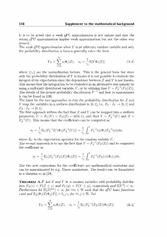
148 Supplement to the mathematical background
It is to be noted that a weak gPC approximation is not unique and that thestrong gPC approximation implies weak approximation but not the other wayaround.The weak gPC approximation when Y is an arbitrary random variable and onlythe probability distribution is known generally takes the form
YN =
N∑i=0
aiΦi(Z), ai =1
γiE[Y Φi(Z)]. (A.4)
where γi are the normalization factors. This is the general form but sinceonly the probability distribution of Y is known it is not possible to evaluate theintegral of the expectation since the dependence between Z and Y is not known.This means that the integral has to be evaluated in an alternative way namely byusing a uniformly distributed variable, U , or by utilizing that Y = F−1
Y (FZ(Z)).The details of the inverse probability distribution F−1 and how to approximateit can be found in [19].The basis for the two approaches is that the probability distribution for Z andY map the variables to a uniform distribution in [0, 1], i.e. FY : IY → [0, 1] andFZ : IZ → [0, 1].The rst approach utilizes the fact that Z and Y can be mapped into a uniformparameter, U = FY (Y ) = FZ(Z) ∼ U(0, 1), and that Y = F−1
Y (U) and Z =F−1Z (U). This means that the coecients can be computed as
ai =1
γiEU [F−1
Y (U)Φi(F−1Z (U))] =
1
γi
∫ 1
0
F−1Y (u)Φi(F
−1Z (u))du,
where EU is the expectation operator for the random variable U .The second approach is to use the fact that Y = F−1
Y (FZ(Z)) and to computedthe coecient as
ai =1
γiEU [F−1
Y (FZ(Z))Φi(Z)] =1
γi
∫ 1
0
F−1Y (FZ(z))Φi(z)dz.
The two new expressions for the coecients are mathematical equivalent andcan be approximated by e.g. Gauss quadrature. The results can be formulatedin a theorem as in [19].
Theorem A.7 Let Z and Y be a random variables with probability distribu-tion FZ(z) = P (Z ≤ z) and FY (y) = P (Y ≤ y), respectively and E[Y 2] < ∞.Furthermore let E[|Z|2m] < ∞ for ∀m ∈ N such that the gPC basis functionsexist and EZ [Φi(Z)Φj(Z)] = δi,jγi for ∀i, j ∈ N. Let
YN =
N∑i=0
aiΦi(Z), ai =1
γiEU [F−1
Y (FZ(Z))Φi(Z)]. (A.5)

A.5 Introduction of strong and weak gPC approximation 149
Then the weak approximation YN converges in probability, i.e. YNP−→ Y for
N →∞, and convergence in distribution, i.e. YNd−→ Y .
The proof of the theorem can be found in [19].

150 Supplement to the mathematical background

Appendix B
Matlab
This appendix contains the Matlab implementations used in the thesis. Theimplementations follows the theory and the algorithms described in the thesis.
B.1 Toolbox
B.1.1 Polynomials and quadratures
B.1.1.1 Implementation of polynomials
The Hermite polynomials are implemented as
1 f unc t i on [ HerPolEx ,w] = HermitePol (x , n , type )2 %3 % Syntax : [ HerPolEx ,w] = HermitePol (x , n , type )4 %5 % Purpose : Compute the n ' th order Hermite polynomial in
the nodes x .6 %7 % input :

152 Matlab
8 % n Order o f the Hermite polynomial .9 %
10 % x The nodes in which the Laguerrepoynomial i s to be
11 % evaluated .12 %13 % type The type o f Hermite polynomial to be
used . type = 114 % r e f e r s to He(x ) which i s the most
r e l e van t f o r t h i s15 % th e s i s .16 %17 %18 % Output19 % HerPolEx A vecto r conta in ing Hermite
polynomial o f order n20 % evaluated in the nodes x .21 %22
23 [ a b ] = s i z e ( x ) ;24 i f a > b25 x = x ' ;26 end27
28 i f type == 129
30 w = 1/ sq r t ( p i ∗2) ∗exp(−x .^2/2) ;31
32 m = [ 0 : f l o o r (n/2) ] ' ; nMinus2m = n−2∗m;33 f r a c t i o n = (−1) .^m. / ( f a c t o r i a l (m) .∗2 .^m.∗ f a c t o r i a l (
nMinus2m) ) ;34
35 XRep = ( repmat (x , l ength ( f r a c t i o n ) ,1 ) ) ' ;36
37 XRepFixed = ze ro s ( s i z e (XRep) ) ;38
39 f o r i = 1 : l ength ( f r a c t i o n )40 XRepFixed ( : , i ) = XRep ( : , i ) .^nMinus2m( i ) ;41 end42
43 HerPolEx = f a c t o r i a l (n ) ∗XRepFixed∗ f r a c t i o n ;44
45 e l s e46 w = 1/ sq r t ( p i ) ∗exp(−x .^2) ;

B.1 Toolbox 153
47 x2 = 2∗x ;48 m = [ 0 : f l o o r (n/2) ] ' ; nMinus2m = n−2∗m;49 f r a c t i o n = (−1) .^m. / ( f a c t o r i a l (m) .∗ f a c t o r i a l (nMinus2m
) ) ;50
51 XRep = ( repmat ( x2 , l ength ( f r a c t i o n ) ,1 ) ) ' ;52
53 XRepFixed = ze ro s ( s i z e (XRep) ) ;54
55 f o r i = 1 : l ength ( f r a c t i o n )56 XRepFixed ( : , i ) = XRep ( : , i ) .^nMinus2m( i ) ;57 end58
59 HerPolEx = f a c t o r i a l (n ) ∗XRepFixed∗ f r a c t i o n ;60
61 end
A recursive implementation have been made that returns Hermite all the Her-mite polynomials in a range of polynomial orders. This has been implementedas
1 f unc t i on [ HerPolEx ] = HermitePolRec (x , type , From ,To)2 %3 % Syntax : [ HerPolEx ] = HermitePolRec (x , type , From ,To)4 %5 % Purpose : Compute the Hermite polynomial from order
From to order To in6 % the nodes x .7 %8 % input :9 % x The nodes in which the polynomia l s
are to be10 % evaluated .11 %12 % type The type o f Hermite polynomial to be
used . type = 113 % r e f e r s to He(x ) which i s the most
r e l e van t f o r t h i s14 % th e s i s .15 %16 % From The lowest order polynomial to be
eva luated .17 %

154 Matlab
18 % To The h ighe s t order polynomial to beeva luated .
19 %20 % Output21 % HerPolEx A matrix conta in ing Hermite
polynomia ls22 % evaluated in the nodes x .23 %24
25 % Help v a r i a b l e s26 Dif = To−From+1;27 xL = length (x ) ;28
29 % I n i t i a l Polynomial30 HerPolEx = ze ro s (xL , Di f ) ;31 i f From <=132 k=1;33 i f From < 134 HerPolEx ( : , 1 ) = ones (xL , 1 ) ;35 k=k+1;36 end37 i f Dif>138 i f type ==139 HerPolEx ( : , k ) = x ;40 e l s e41 HerPolEx ( : , k ) = 2∗x ;42 end43 end44 e l s e45 n = From+2;46 i f Dif>=247 [w, HerPolEx ( : , 1 ) ] = HermitePol (x , From , type ) ;48 [w, HerPolEx ( : , 2 ) ] = HermitePol (x , From+1, type ) ;49 e l s e50 [w, HerPolEx ( : , 1 ) ] = HermitePol (x , From , type ) ;51 end52 end53 n = From+1;54 i f Dif>255 f o r k = 3 : Di f56 HerPolEx ( : , k ) = x ' . ∗ HerPolEx ( : , k−1)−n∗HerPolEx ( : ,
k−2) ;57 n = n+1;58 end
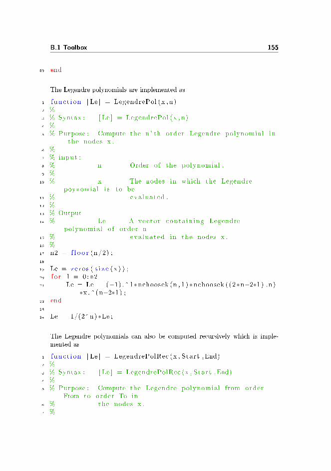
B.1 Toolbox 155
59 end
The Legendre polynomials are implemented as
1 f unc t i on [ Le ] = LegendrePol (x , n)2 %3 % Syntax : [ Le ] = LegendrePol (x , n )4 %5 % Purpose : Compute the n ' th order Legendre polynomial in
the nodes x .6 %7 % input :8 % n Order o f the polynomial .9 %
10 % x The nodes in which the Legendrepoynomial i s to be
11 % evaluated .12 %13 % Output14 % Le A vecto r conta in ing Legendre
polynomial o f order n15 % evaluated in the nodes x .16 %17 n2 = f l o o r (n/2) ;18
19 Le = ze ro s ( s i z e ( x ) ) ;20 f o r l = 0 : n221 Le = Le + (−1) .^ l ∗nchoosek (n , l ) ∗nchoosek ((2∗n−2∗ l ) ,n )
∗x .^(n−2∗ l ) ;22 end23
24 Le = 1/(2^n) ∗Le ;
The Legendre polynomials can also be computed recursively which is imple-mented as
1 f unc t i on [ Le ] = LegendrePolRec (x , Start , End)2 %3 % Syntax : [ Le ] = LegendrePolRec (x , Start , End)4 %5 % Purpose : Compute the Legendre polynomial from order
From to order To in6 % the nodes x .7 %

156 Matlab
8 % input :9 % x The nodes in which the polynomia l s
are to be10 % evaluated .11 %12 % Star t The lowest order polynomial to be
eva luated .13 %14 % End The h ighe s t order polynomial to be
eva luated .15 %16 % Output17 % Le A matrix conta in ing Legendre
polynomia ls18 % evaluated in the nodes x .19 %20
21 Len = abs (End−Star t )+1;22
23 Le0 = ones ( s i z e ( x ) ) ;24 Le1 = x ;25
26 Le = ze ro s ( l ength (x ) , Len ) ;27 i f S ta r t == 028 Le ( : , 1 ) = Le0 ;29 i f Len >= 230 Le ( : , 2 ) = Le1 ;31 end32 e l s e i f S ta r t == 133 Le ( : , 1 ) = Le1 ;34 i f Len >= 235 Le ( : , 2 ) = 1/2∗(3∗x^2−1) ;36 end37 e l s e38 Le ( : , 1 ) = LegendrePol (x , S ta r t ) ;39
40 i f Len >=241 Le ( : , 2 ) = LegendrePol (x , S ta r t+1) ;42 end43 end44
45 i f Len>=346 f o r k = 2 : Len−147 n = Star t+k−1;
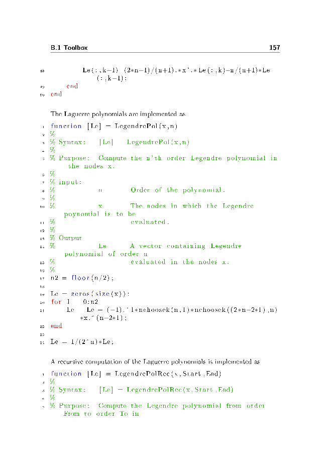
B.1 Toolbox 157
48 Le ( : , k+1)=(2∗n+1)/(n+1) .∗ x ' . ∗ Le ( : , k )−n/(n+1)∗Le( : , k−1) ;
49 end50 end
The Laguerre polynomials are implemented as
1 f unc t i on [ Le ] = LegendrePol (x , n )2 %3 % Syntax : [ Le ] = LegendrePol (x , n )4 %5 % Purpose : Compute the n ' th order Legendre polynomial in
the nodes x .6 %7 % input :8 % n Order o f the polynomial .9 %
10 % x The nodes in which the Legendrepoynomial i s to be
11 % evaluated .12 %13 % Output14 % Le A vecto r conta in ing Legendre
polynomial o f order n15 % evaluated in the nodes x .16 %17 n2 = f l o o r (n/2) ;18
19 Le = ze ro s ( s i z e ( x ) ) ;20 f o r l = 0 : n221 Le = Le + (−1) .^ l ∗nchoosek (n , l ) ∗nchoosek ( (2∗n−2∗ l ) ,n )
∗x .^(n−2∗ l ) ;22 end23
24 Le = 1/(2^n) ∗Le ;
A recursive computation of the Laguerre polynomials is implemented as
1 f unc t i on [ Le ] = LegendrePolRec (x , Start , End)2 %3 % Syntax : [ Le ] = LegendrePolRec (x , Start , End)4 %5 % Purpose : Compute the Legendre polynomial from order
From to order To in

158 Matlab
6 % the nodes x .7 %8 % input :9 % x The nodes in which the polynomia l s
are to be10 % evaluated .11 %12 % Star t The lowest order polynomial to be
eva luated .13 %14 % End The h ighe s t order polynomial to be
eva luated .15 %16 % Output17 % Le A matrix conta in ing Legendre
polynomia ls18 % evaluated in the nodes x .19 %20
21 Len = abs (End−Star t )+1;22
23 Le0 = ones ( s i z e ( x ) ) ;24 Le1 = x ;25
26 Le = ze ro s ( l ength (x ) , Len ) ;27 i f S ta r t == 028 Le ( : , 1 ) = Le0 ;29 i f Len >= 230 Le ( : , 2 ) = Le1 ;31 end32 e l s e i f S ta r t == 133 Le ( : , 1 ) = Le1 ;34 i f Len >= 235 Le ( : , 2 ) = 1/2∗(3∗x^2−1) ;36 end37 e l s e38 Le ( : , 1 ) = LegendrePol (x , S ta r t ) ;39
40 i f Len >=241 Le ( : , 2 ) = LegendrePol (x , S ta r t+1) ;42 end43 end44
45 i f Len>=3

B.1 Toolbox 159
46 f o r k = 2 : Len−147 n = Star t+k−1;48 Le ( : , k+1)=(2∗n+1)/(n+1) .∗ x ' . ∗ Le ( : , k )−n/(n+1)∗Le
( : , k−1) ;49 end50 end
The derivatives of the Jacobi polynomials are implemented as
1 f unc t i on [Pm] = GradJacobiPoln (x , alpha , beta ,N)2 %3 % Syntax : [Pm] = GradJacobiPoln (x , alpha , beta ,N)4 %5 % Purpose : Compute the grad iant to the n ' th order Jacobi
polynomial6 % in the nodes x .7 %8 % input :9 % N Order o f the polynomial .
10 %11 % x The nodes in which the Legendre
poynomial i s to be12 % evaluated .13 %14 % alpha The alpha value used to d e f i n e the
Jacobi polynomial15 %16 % beta The beta value used to d e f i n e the
Jacobi polynomial17 %18 % Output19 % Pm A vector conta in ing grad iant
polynomial eva luated in20 % the nodes x .21 %22
23 i f N==0;24 Pm = zero s ( s i z e ( x ) ) ;25 e l s e26 [P ] = JacobiPolNorm (x , alpha+1, beta+1,N−1) ;27 Pm = zero s ( l ength (x ) ) ;28 f o r n i = 1 :N29 Pm( : , n i+1) = sq r t ( n i ∗( n i+alpha+beta+1) ) ∗P( : , n i ) ;30 end

160 Matlab
31 end
The normalized Jacobi polynomials are used and the implementation for theseare given in
1 f unc t i on [ p ] = JacobiPolNorm (x , alpha , beta ,N)2 %3 % Syntax : [ p ] = JacobiPolNorm (x , alpha , beta ,N)4 %5 % Purpose : Compute the the n ' th order normal ized Jacobi
polynomial6 % in the nodes x .7 %8 % input :9 % N Order o f the polynomial .
10 %11 % x The nodes in which the Legendre
polynomial i s to be12 % evaluated .13 %14 % alpha The alpha value used to d e f i n e the
Jacobi polynomial15 %16 % beta The beta value used to d e f i n e the
Jacobi polynomial17 %18 % Output19 % p A vector conta in ing polynomial
eva luated in20 % the nodes x .21 %22
23 % Ensure that x i s a column and not a row vecto r .24 x = x ( : ) ;25
26 P = ze ro s ( l ength (x ) ,N+1) ;27 PN = P;28
29 P( : , 1 ) = 1 ;30
31 gamma1 = 2^( alpha+beta+1)∗ f a c t o r i a l (0+alpha ) ∗ f a c t o r i a l (0+beta ) ;
32 gamma2 = f a c t o r i a l (0 ) ∗(0+alpha+beta+1)∗ f a c t o r i a l (0+alpha+beta ) ;

B.1 Toolbox 161
33 gammaInv0 = gamma2/gamma1 ;34
35 PN( : , 1 ) = sq r t (gammaInv0) ∗P( : , 1 ) ;36
37
38 i f N == 039 p = PN( : , 1 ) ;40 re turn41 e l s e i f (N==−1)42 p = PN( : , 1 ) ∗0 ;43 re turn44 end45
46 P( : , 2 ) = 1/2∗( alpha−beta ) + 1/2∗( alpha+beta+2)∗x ;47
48 gamma1 = 2^( alpha+beta+1)∗ f a c t o r i a l (1+alpha ) ∗ f a c t o r i a l (1+beta ) ;
49 gamma2 = f a c t o r i a l (1 ) ∗(2+alpha+beta+1)∗ f a c t o r i a l (1+alpha+beta ) ;
50 gammaInv = gamma2/gamma1 ;51
52 PN( : , 2 ) = sq r t (gammaInv) ∗P( : , 2 ) ;53
54
55 i f N ==156 p = P;57 re turn ;58 end59
60 f o r n = 1 :N−161 re = 2∗n+alpha+beta ; % Factor computed once and
reused .62 Pn1 = 2∗(n+alpha ) ∗(n+beta ) / ( ( re+1)∗ re ) ∗P( : , n ) ;63 Pn = ( ( alpha^2−beta ^2) / ( ( re+2)∗ re ) + x) .∗P( : , n+1) ;64 InvFac = ( ( re+2)∗( re+1) ) /(2∗ ( n+1)∗( re−n+1) ) ;65
66 P( : , n+2) = InvFac ∗(Pn − Pn1) ;67
68 n2 = n+1;69
70 gamma1 = 2^( alpha+beta+1)∗ f a c t o r i a l ( n2+alpha ) ∗f a c t o r i a l ( n2+beta ) ;
71 gamma2 = f a c t o r i a l ( n2 ) ∗(2∗n2+alpha+beta+1)∗ f a c t o r i a l (n2+alpha+beta ) ;
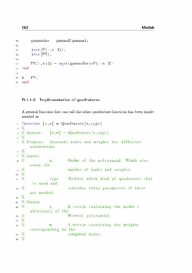
162 Matlab
72 gammaInv = gamma2/gamma1 ;73
74 s i z e (P( : , n+2) ) ;75 s i z e (PN) ;76
77 PN( : , n+2) = sq r t (gammaInv) ∗P( : , n+2) ;78 end79
80 p = PN;81 end
B.1.1.2 Implementation of quadratures
A general function that can call the other quadrature functions has been imple-mented as
1 f unc t i on [ x ,w] = Quadrature (n , type )2 %3 % Syntax : [ x ,w] = Quadrature (n , type )4 %5 % Purpose : Generate nodes and weights f o r d i f f e r e n t
quadratures6 %7 % input :8 % n Order o f the polynomial . Which a l s o
means the9 % number o f nodes and weights .
10 %11 % type De f ines which kind o f quadrature that
i s used and12 % conta in s ext ra parameters i f the se
are needed .13 %14 % Output15 % x A vector conta in ing the nodes (
a b s c i s s a s ) o f the16 % Hermite polynomial .17 %18 % w A vector conta in ing the weights
corre spond ing to the19 % computed nodes .20 %
B.1 Toolbox 163
21
22 i f strcmp ( type (1 ) , ' hermite ' )23
24 [ x ,w] = HermiteQuad (n) ;25
26 e l s e i f strcmp ( type (1 ) , ' l a gu e r r e ' )27
28 [ x ,w] = laguerrequad (n) ;29
30 e l s e i f strcmp ( type (1 ) , ' l e g endre ' )31
32 [ x ,w] = legendrequad (n) ;33
34 e l s e i f strcmp ( type (1 ) , ' l e g e n d r e s h i f t ' )35
36 [ x ,w] = legendrequad01 (n) ;37
38 e l s e i f strcmp ( type (1 ) , ' j a c ob i ' )39
40 [ x ,w] = JacobiGQ( type (2 ) , type (3 ) ,n ) ;41 end
The Gauss Hermite quadrature is implemented as
1 f unc t i on [ x ,w] = HermiteQuad (n)2 %3 % Syntax : [ x ,w] = HermiteQuad (n)4 %5 % Purpose : Generate nodes and weights f o r Gauss Hermite
quadrature .6 %7 % input :8 % n Order o f the polynomial . Which a l s o
means the9 % number o f nodes and weights .
10 %11 % Output12 % x A vector conta in ing the nodes (
a b s c i s s a s ) o f the13 % Hermite polynomial .14 %15 % w A vector conta in ing the weights
corre spond ing to the16 % computed nodes .
164 Matlab
17 %18
19 nV = 1 : n−1;20 BetaSqrt = sq r t (nV. / 2 ) ;21 J = diag ( BetaSqrt , 1 )+diag ( BetaSqrt ,−1) ;22 [V,D] = e i g ( J ) ;23 [ x , ind ] = so r t ( diag (D) ) ;24 wTemp = sq r t ( p i ) ∗V( 1 , : ) . ^ 2 ;25 w = wTemp( ind ) ;
The computation of the Gauss Legendre quadrature nodes and weights is im-plemented as
1 f unc t i on [ x ,w] = legendrequad (n)2 %3 % Syntax : [ x ,w] = legendrequad (n)4 %5 % Purpose : Generate nodes and weights f o r Gauss Legendre
quadrature .6 %7 % input :8 % n Order o f the polynomial . Which a l s o
means the9 % number o f nodes and weights .
10 %11 % Output12 % x A vector conta in ing the nodes (
a b s c i s s a s ) o f the13 % Hermite polynomial .14 %15 % w A vector conta in ing the weights
corre spond ing to the16 % computed nodes .17 %18 u = sq r t ( 1 . / ( 4 −1 . / [ 1 : n−1] .^2) ) ; % upper diag .19 [V, Lambda ] = e i g ( diag (u , 1 )+diag (u,−1) ) ;20 [ x , i ] = s o r t ( diag (Lambda) ) ;21 Vtop = V( 1 , : ) ;22 Vtop = Vtop ( i ) ;23 w = 2∗Vtop .^2 ;
The implementation of the shifted Gauss Legendre quadrature nodes and weightsis

B.1 Toolbox 165
1 f unc t i on [ x ,w] = legendrequad01 (n)2 %3 % Syntax : [ x ,w] = legendrequad01 (n)4 %5 % Purpose : Generate nodes and weights f o r the s h i f t e d
Gauss Legendre6 % quadrature i . e . in the i n t e r v a l [ 0 , 1 ] .7 %8 % input :9 % n Order o f the polynomial . Which a l s o
means the10 % number o f nodes and weights .11 %12 % Output13 % x A vector conta in ing the nodes (
a b s c i s s a s ) o f the14 % Hermite polynomial .15 %16 % w A vector conta in ing the weights
corre spond ing to the17 % computed nodes .18 %19 a = repmat (1/2 ,1 , n ) ; % main d iagona l o f J20 u = sq r t ( 1 . / ( 4∗ ( 4 −1 . / [ 1 : n−1] .^2) ) ) ;21 [V, Lambda ] = e i g ( diag (u , 1 )+diag ( a )+diag (u,−1) ) ;22 [ x , i ] = s o r t ( diag (Lambda) ) ;23 Vtop = V( 1 , : ) ;24 Vtop = Vtop ( i ) ;25 w = Vtop .^2 ;
The Gauss Laguerre quadrature rule is implemented as
1 f unc t i on [ x ,w] = laguerrequad (n)2 %3 % Syntax : [ x ,w] = laguerrequad (n)4 %5 % Purpose : Generate nodes and weights f o r Gauss Laguerre
quadrature .6 %7 % input :8 % n Order o f the polynomial . Which a l s o
means the9 % number o f nodes and weights .
10 %

166 Matlab
11 % Output12 % x The nodes ( a b s c i s s a s ) o f the Hermite
polynomial .13 %14 % w The weights cor re spond ing to the
computed15 % nodes .16 %17
18 a = 2 ∗ [ 0 : n−1]+1; % diagona l o f J19 u = [ 1 : n−1] ; % upper d iagona l o f J20 [V, Lambda ] = e i g ( diag (u , 1 )+diag ( a )+diag (u,−1) ) ;21 [ x , i ] = s o r t ( diag (Lambda) ) ;22 Vtop = V( 1 , : ) ;23 Vtop = Vtop ( i ) ;24 w = Vtop .^2 ;
The Gauss-Lobatto nodes are implemented as
1 f unc t i on [ x ] = JacobiGL ( alpha , beta ,N)2
3 % func t i on [ x ] = JacobiGL ( alpha , beta ,N)4 % Purpose : Compute the N' th order Gauss Lobatto
quadrature5 % points , x , a s s o c i a t ed with the Jacobi
polynomial ,6 % of type ( alpha , beta ) > −1 ( <> −0.5) .7
8 x = ze ro s (N+1 ,1) ;9 i f (N==1) x (1 ) =−1.0; x (2 ) =1.0 ; r e turn ; end ;
10
11 [ x int ,w] = JacobiGQ( alpha+1, beta+1,N−2) ;12 x = [−1 , xint ' , 1 ] ' ;13 re turn ;
The implementation of the Gauss-Lobatto nodes relies on the implementationof the Gauss Quadrature points implemented as
1 f unc t i on [ x ,w] = JacobiGQ( alpha , beta ,N)2
3 % func t i on [ x ,w] = JacobiGQ( alpha , beta ,N)4 % Purpose : Compute the N' th order Gauss quadrature points
, x ,5 % and weights , w, a s s o c i a t ed with the Jacobi

B.1 Toolbox 167
6 % polynomial , o f type ( alpha , beta ) > −1 ( <>−0.5) .
7
8 i f (N==0) x (1 )=(alpha−beta ) /( alpha+beta+2) ; w(1 ) = 2 ;re turn ; end ;
9
10 % Form symmetric matrix from recur r ence .11 J = ze ro s (N+1) ;12 h1 = 2∗ ( 0 :N)+alpha+beta ;13 J = diag (−1/2∗( alpha^2−beta ^2) . / ( h1+2) . / h1 ) + . . .14 diag ( 2 . / ( h1 ( 1 :N)+2) .∗ s q r t ( ( 1 :N) . ∗ ( ( 1 :N)+alpha+beta )
. ∗ . . .15 ( ( 1 :N)+alpha ) . ∗ ( ( 1 :N)+beta ) . / ( h1 ( 1 :N)+1) . / ( h1 ( 1 :N)+3)
) ,1 ) ;16 i f ( alpha+beta <10∗eps ) J (1 , 1 ) =0.0 ; end ;17 J = J + J ' ;18
19 %Compute quadrature by e i g enva lue s o l v e20 [V,D] = e i g ( J ) ; x = diag (D) ;21 w = (V( 1 , : ) ' ) .^2∗2^( alpha+beta+1)/( alpha+beta+1)∗gamma(
alpha+1) ∗ . . .22 gamma( beta+1)/gamma( alpha+beta+1) ;23 re turn ;
B.1.2 Vandermonde-like matrices.
The implementation of the Vandermonde-like matrix V is given by
1 f unc t i on D = JacobiDn (x , alpha , beta )2
3 % Compute the g en e r a l i z e d Vandermonde matr i ce s V and Vx4 N = length (x ) ;5 %V = JacobiPolNorm (x , alpha , beta ,N−1) ;6
7 V = JacobiPolNorm (x , alpha , beta ,N−1) ;8 Vx = GradJacobiPoln (x , alpha , beta ,N−1) ;9
10 % The i nv e r s e matrix o f V i s computed11 D = Vx/V;

168 Matlab
B.1.3 ERK
The implementation of the explicit Runge-Kutta method is given here
1 f unc t i on U = ERK( t ,U, fun , dt , param)2
3 G = U;4 P = f e v a l ( fun , t ,U, param) ;5 U = U + 0.5∗ dt∗P;6 G = P;7 P = f e v a l ( fun , t +0.5∗dt ,U, param) ;8 U = U + 0.5∗ dt ∗(P−G) ;9 G = (1/6) ∗G;
10 P = f e v a l ( fun , t +0.5∗dt ,U, param) − 0 .5∗P;11 U = U + dt∗P;12 G = G − P;13 P = f e v a l ( fun , t+dt ,U, param) +2∗P;14 U = U + dt ∗(G + (1/6) ∗P) ;
B.2 Test Equation
B.2.1 Monte Carlo
A test script for the Monte Carlo simulation for the Test Equation has beenimplemented as
1 %%%%%%%%%%%%%%%%%%%%%%%%%%%%%%%%%%%%%%%%%%%%%%%%%%%%%%%%%%%%%%%%%%%%%%%%%%%
2 %%%%%% Monte Carlo Sc r i p t%%%%%%
3 %%%%%% Vers ion 1 .0
%%%%%%4 %%%%%% Author : Emil Brandt Kaergaard
%%%%%%5 %
%%%%%%%%%%%%%%%%%%%%%%%%%%%%%%%%%%%%%%%%%%%%%%%%%%%%%%%%%%%%%%%%%%%%%%%%%%
6
7

B.2 Test Equation 169
8 % Parameters : The s i z e o f the dataset , the weight o f thes o l u t i on s ,
9 % the number o f dataset s , the type o f d i s t r i b u t i o n andparameters s p e c i f i c
10 % fo r the d i s t r i b u t i o n .11
12 c l o s e a l l ; c l e a r a l l ;13
14
15 % Number o f r e a l i z a t i o n s , time−endpoint16 N = [100 1000 5000 10000 30000 50000 80000 100000 150000
300000 500000 800000 1000000 ] ;17
18 Ns = 1 ./ sq r t (N) ;19 tend = 1 ; tN = 45 ;20
21 % Computing the parameters f o r gene ra t ing the randomva r i a b l e s .
22 mu = 0 ; sigma = sq r t ( 0 . 2 5 ) ;23 Alpha . DistType = ' normal ' ;24 Alpha .Dim = [ 1 , 1 ] ;25 Alpha . Par = [mu, sigma ] ;26
27 Beta = 1 ;28 RealSol = 2 ;29 MuEx = exp ( tend ^2/2) ;30
31 % Pre−a l l o c a t i o n32 Mu = ze ro s ( tN , l ength (N) ) ;33 Sigma = ze ro s ( tN , l ength (N) ) ;34 MuExact = ze ro s ( tN , l ength (N) ) ;35 SigmaExact = ze ro s ( tN , l ength (N) ) ;36 MuErr = ze ro s ( tN , l ength (N) ) ;37 SigErr = ze ro s ( tN , l ength (N) ) ;38 Time = ze ro s (1 , l ength (N) ) ;39
40 f o r k =1: l ength (N)41 [Mu( : , k ) , Sigma ( : , k ) ,CI , Exact , Err , Time(k ) ] =
MCTestEqSolv (Alpha , Beta , tend , tN ,N(k ) , RealSol ) ;42 MuExact ( : , k ) = Exact .MuExact ;43 SigmaExact ( : , k ) = Exact . SigmaExact ;44 MuErr ( : , k ) = Err .MuErr ;45 SigErr ( : , k ) = Err . S igErr ;46 Time(k )

170 Matlab
47 end48
49 t = l i n s p a c e (0 , tend , tN) ;50
51 f i g u r e (1 )52 hold on53 p lo t ( t ,Mu( : , end ) , 'b−∗ ' , t , CI .UB, 'k−∗ ' , t , CI .LB, 'k−∗ ' )54 p lo t ( t ,MuExact , ' r−o ' , t , Exact . UBExact , ' g−o ' , t , Exact .
LBExact , ' g−o ' )55 hold o f f
Much of the computations have been implemented in
1 f unc t i on [Mu, Sigma , CI , Exact , Err , Time , t ] = MCTestEqSolv (Alpha , Beta , tend , tN ,M, RealSol )
2 %3 % Function f o r us ing Monte Carlo method on Test Equation .4 % Vers ion 1 .05 % Author : Emil Brandt Kaergaard6 %7 % Syntax :8 % [Mu, Sigma , CI , Exact , Err ] = MCTestEqSolv (Alpha ,
Beta , tend , tN ,M)9 %
10 %11
12 % Computing the parameters alpha and beta .13 alpha = RandVar (Alpha . DistType , Alpha .Dim,M, Alpha . Par ) ;14 i f l ength ( Beta ) == 115 beta = Beta∗ ones (1 ,M) ;16 e l s e17 beta = RandVar ( Beta . DistType , Beta .Dim,M, Beta . Par ) ;18 end19
20 % Computing the tspan and p r e a l l o c a t i n g a matrix U f o rthe s o l u t i o n s u f o r
21 % the d e t e rm i n i s t i c s o l u t i o n o f each r e a l i z a t i o n o f the (pseudo−)random parameters .
22 tspan = l i n s p a c e (0 , tend , tN) ;23 dt = abs ( tspan (2 )−tspan (1 ) ) ;24 U = zero s ( l ength ( tspan ) ,M) ;25
26 i f RealSol == 127 t = tspan ' ;

B.2 Test Equation 171
28 t i c29 f o r i =1:M30 U( : , i ) = exp(−alpha ( i ) .∗ t ) ;31 end32 Time = toc ;33 e l s e i f RealSol == 034 t i c35 f o r i =1:M36 [ t ,U( : , i ) ] = ode45 (@TestEq , tspan , beta ( i ) , [ ] , a lpha
( i ) ) ;37 end38 Time = toc ;39
40 e l s e41 t = ze ro s ( s i z e ( tspan ) ) ;42 t i c43 f o r i =1:M44 U(1 , i )=beta ( i ) ;45 f o r t i = 2 : l ength ( tspan )46 U( t i , i ) = ERK( tspan ( t i ) ,U( t i −1, i ) ,@TestEq , dt ,
alpha ( i ) ) ;47 t ( t i )=t ( t i −1)+dt ;48 end49 end50 Time = toc ;51 t = t ' ;52 end53 % Computing modes : Mean and var iance .54 Mu = sum(U, 2 ) /M;55
56 Sig = ze ro s ( l ength ( tspan ) ,M) ;57 f o r k = 1 :M58 Sig ( : , k ) = (U( : , k )−Mu) .^2 ;59 end60
61 Sigma = sum( Sig , 2 ) /(M−1) ;62
63 UB = Mu + 1.96∗ s q r t ( Sigma ) / sq r t (M) ;64 LB = Mu − 1 .96∗ s q r t ( Sigma ) / sq r t (M) ;65
66 CI .UB = UB;67 CI .LB = LB;68
69 % Coumpitng exact va lue s i f the se are known .
172 Matlab
70 i f strcmp (Alpha . DistType , ' normal ' )71 MuExact = exp (1/2 .∗ ( Alpha . Par (2 ) .∗ t ) .^2−Alpha . Par (1 )
.∗ t ) ;72 SigmaExact = exp (2∗ ( Alpha . Par (2 ) .∗ t ) .^2−2∗Alpha . Par
(1 ) .∗ t )−exp ( ( Alpha . Par (2 ) .∗ t ) .^2−2∗Alpha . Par (1 ) .∗ t) ;
73
74 UBExact = MuExact + 1.96∗ s q r t ( SigmaExact ) / sq r t (M) ;75 LBExact = MuExact − 1 .96∗ s q r t ( SigmaExact ) / sq r t (M) ;76
77 MuErr = abs (Mu − MuExact ) ;78 SigErr = abs ( Sigma − SigmaExact ) ;79 e l s e i f strcmp (Alpha . DistType , ' uniform ' )80 MuExact = −(exp(−(Alpha . Par (2 ) .∗ t ) )−exp(−(Alpha . Par
(1 ) .∗ t ) ) ) . / ( t . ∗ ( Alpha . Par (2 )−Alpha . Par (1 ) ) ) ;81 SigmaExact = −(exp(−2∗(Alpha . Par (2 ) .∗ t ) )−exp(−2∗(
Alpha . Par (1 ) .∗ t ) ) ) . / ( 2∗ t . ∗ ( Alpha . Par (2 )−Alpha . Par(1 ) ) )−MuExact . ^2 ;
82
83 UBExact = MuExact + 1.96∗ s q r t ( SigmaExact ) / sq r t (M) ;84 LBExact = MuExact − 1 .96∗ s q r t ( SigmaExact ) / sq r t (M) ;85
86 MuErr = abs (Mu − MuExact ) ;87 SigErr = abs ( Sigma − SigmaExact ) ;88
89 e l s e90
91 MuExact = 0 ;92 SigmaExact = 0 ;93
94 UBExact = 0 ;95 LBExact = 0 ;96
97 MuErr = 0 ;98 SigErr = 0 ;99 end
100
101 Exact .MuExact = MuExact ;102 Exact . SigmaExact = SigmaExact ;103 Exact . UBExact = UBExact ;104 Exact . LBExact = LBExact ;105
106 Err .MuErr = MuErr ;107 Err . S igErr = SigErr ;

B.2 Test Equation 173
The random variables are computed by using the following implementation
1 f unc t i on X = RandVar (DistType ,Dim,M, Par )2 %3 % Random Var iabe l S c r i p t4 % Vers ion 1 .05 % Date : December 20126 % Author : Emil Brandt Kaergaard7 %8 % RandVar :9 % This func t i on computes M random va r i a b l e s o f
dimension Dim . The10 % type o f d i s t r i b u t i o n used to generate the
v a r i a b l e s i s de f in ed11 % in DistType and by the parameters in Par .12 %13 % Syntax :14 % X = RandVar (DistType ,Dim,M, Par )15 %16 % Input :17 % DistType : The type o f d i s t r i b u t i o n used to
generate the18 % va r i a b l e s .19 % Dim: Dimension o f the v a r i a b l e s .20 % M: Number o f random va r i a b l e s .21 % Par : The parameters o f the chosen
d i s t r i b u t i o n o f the v a r i a b l e s .22 %23 % Output :24 % X: A Dim x M matrix conta in ing M ( pseudo−)
random va r i a b l e s o f dimension Dim .25 %26
27
28 % Def in ing row− and column−l ength .29 row = Dim(1) ;30 column = Dim(2) ;31
32 % I n i t i a l i z e parameters33 i f l ength (Par ) == 1 % Use d e f au l t d i s t r i b u t i o n parameters
.34 i f strcmp (DistType , ' normal ' )35 mu = 0 ;36 sigma = 1 ;

174 Matlab
37 e l s e i f strcmp (DistType , ' uniform ' )38 a = −1;39 b = 1 ;40 end41 e l s e i f l ength (Par ) == 2 % Use user−de f ined parameters42 i f strcmp (DistType , ' normal ' )43 mu = Par (1 ) ;44 sigma = Par (2 ) ;45 e l s e i f strcmp (DistType , ' uniform ' )46 a = Par (1 ) ;47 b = Par (2 ) ;48 end49 end50
51 % Generating random samples52
53 i f strcmp (DistType , ' normal ' )54 X = mu + sigma .∗ randn ( row , column ,M) ;55 e l s e i f strcmp (DistType , ' uniform ' )56 X = a + (b−a ) .∗ rand ( row , column ,M) ;57 e l s e58 e r r o r ( 'Wrong type o f d i s t r i b u t i o n ' )59 end
The rhs-function has been implemented as
1 f unc t i on du = TestEq ( t , u , alpha )2 %3 % Test Equation Sc r i p t .4 % Vers ion 1 .05 % Date : December 20126 % Author : Emil Brandt Kaergaard7 %8 % TestEq :9 %
10 % Syntax :11 % du = TestEq ( t , u , alpha )12 %13 % Input :14 %15 % Output :16 %17
18 du = −alpha .∗u ;

B.2 Test Equation 175
B.2.2 Stochastic Collocation Method
A test script computing following the pseudocode 5 have been implemented as
1 %%%%%%%%%%%%%%%%%%%%%%%%%%%%%%%%%%%%%%%%%%%%%%%%%%%%%%%%%%%%%%%%%%%%%%%%%%%
2 %%%%%%%%% Stocha s t i c Co l l o ca t i on method on the TestEquation . %%%%%%%%%
3 %%%%%%%%% Vers ion 1 .0%%%%%%%%%
4 %%%%%%%%% Date : February 2012%%%%%%%%%
5 %%%%%%%%% Author : Emil Brandt Kaergaard%%%%%%%%%
6 %%%%%%%%%%%%%%%%%%%%%%%%%%%%%%%%%%%%%%%%%%%%%%%%%%%%%%%%%%%%%%%%%%%%%%%%%%%
7
8
9 % Constants :10 zN = 9 ;11 dt = 0 . 0 5 ;12
13 tBeg = 0 ; tEnd = 1 ;14 tspan = tBeg : dt : tEnd ;15
16 DistType = ' uniform ' ;17
18 i f strcmp (DistType , ' normal ' )19 % Gaussian D i s t r i bu t i on : Hermite Gauss Quadrature
nodes .20 mu = 0 ; Var = 1 ; sigma = sq r t (Var ) ;21 par1 = mu; par2 = sigma ;22
23 [ z ,zW] = HermiteQuadN(zN) ; % Computing nodes andweights
24
25 z = mu+sigma∗z ; % Computing the N(mu, sigma )d i s t r i b u t e d alpha−parameter
26 n = 0 : zN−1;27 e l s e i f strcmp (DistType , ' uniform ' )28 % Uniform Di s t r i bu t i on : Legendre Gauss Quadrature
nodes .
176 Matlab
29 [ z ,zW] = legendrequad (zN) ; % Computing nodes andweights
30 zW = 1/2∗zW;31 a = −1; b=1;32 par1 = a ; par2 = b ;33 end34
35 % Pre−a l l o c a t i o n and i n i t i a l c ond i t i on .36 U = zero s (zN , l ength ( tspan ) ) ;37 U( : , 1 ) = ones (zN , 1 ) ;38
39 % Solv ing d e t e rm i n i s t i c system .40 t i c41 f o r t i = 1 : l ength ( tspan )−142 U( : , t i +1) = ERK( tspan ( t i ) ,U( : , t i ) ,@rhsSCMtest , dt , z ) ;43 end44 time = toc ;45
46 f i g u r e47 p lo t ( tspan ,U' )48
49 [Umean , Uvar , MuExact , SigmaExact , MuErr , S igErr ] =TestEqX(DistType , par1 , par2 ,U,zW, zN , tspan ) ;
50
51 f i g u r e52 hold on53 p lo t ( tspan ,Umean( end , : ) , ' b ' )54 p lo t ( tspan ,MuExact , ' r−. ' )55 hold o f f56
57
58 %%59
60 %%%%%%%%%%%%%%%%%%%%%%%%%%%%%%%%%%%%%%%%%%%%%%%%%%%%%%%%%%%%%%%%%%%%%%%%%%%
61 %%%%% Computing e r r o r s f o r d i f f e r e n t zN f o r SCM on theTest Equation . %%%%%
62 %%%%% Vers ion 1 .0
%%%%%63 %%%%% Date : February 2012
%%%%%

B.2 Test Equation 177
64 %%%%% Author : Emil Brandt Kaergaard%%%%%
65 %%%%%%%%%%%%%%%%%%%%%%%%%%%%%%%%%%%%%%%%%%%%%%%%%%%%%%%%%%%%%%%%%%%%%%%%%%%
66
67 % Constants :68 ZN = 16 ; % Maximum number o f nodes and weights in z .69 dt = 0 . 0 0 5 ;70
71 tBeg = 0 ; tEnd = 1 ;72 tspan = tBeg : dt : tEnd ;73
74 DistType = ' normal ' ; % Choice o f d i s t r i b u t i o n o f z .75
76 MuErr = ze ro s (ZN, l ength ( tspan ) ) ;77 SigErr = MuErr ;78
79 f o r zN = 1 :ZN80
81 i f strcmp (DistType , ' normal ' )82 % Gaussian D i s t r i bu t i on : Hermite Gauss Quadrature
nodes .83 mu = 0 ; Var = 1 ; sigma = sq r t (Var ) ;84 par1 = mu; par2 = sigma ;85
86 [ z ,zW] = HermiteQuadN(zN) ;87
88 z = mu+sigma∗z ;89 n = 0 : zN−1;90 e l s e i f strcmp (DistType , ' uniform ' )91 % Uniform Di s t r i bu t i on : Legendre Gauss Quadrature
nodes .92 alpha = 0 ; beta = 0 ;93 [ z ,zW] = JacobiGQ( alpha , beta , zN−1) ;94
95 zW = 1/2∗zW;96 a = −1; b=1;97 par1 = a ; par2 = b ;98 end99
100 % Pre−a l l o c a t i o n and i n i t i a l c ond i t i on .101 U = zero s (zN , l ength ( tspan ) ) ;102 U( : , 1 ) = ones (zN , 1 ) ;

178 Matlab
103
104 % Solv ing the d e t e rm i n i s t i c system .105 t i c106 f o r t i = 1 : l ength ( tspan )−1107 U( : , t i +1) = ERK( tspan ( t i ) ,U( : , t i ) ,@rhsSCMtest , dt ,
z ) ;108 end109 time = toc ;110
111 [Umean , Uvar , MuExact , SigmaExact , MuErr(zN , : ) ,S igErr (zN , : ) ] = TestEqX(DistType , par1 , par2 ,U,zW, zN, tspan ) ;
112 end113
114 f i g u r e115 semi logy ( 1 :ZN,MuErr ( : , end ) , 'b . ' , 1 :ZN, SigErr ( : , end ) , ' ro ' ) ;116
117 f i g u r e118 semi logy ( 1 :ZN, SigErr ( : , end ) ) ;
The rhs-function has been implemented as
1 f unc t i on un = rhsSCMtest ( t ,U, alpha )2
3 un = alpha .∗U;
The approximated and exact statistics are computed in TestEqX which is im-plemented as
1 f unc t i on [Umean , Uvar , MuExact , SigmaExact , MuErr , S igErr] = TestEqX(DistType , par1 , par2 ,U,zW, zN , tspan )
2
3 t = tspan ;4
5 % Computing mean :6 Uw = ze ro s (zN , l ength ( tspan ) ) ;7 f o r z i = 1 : zN8 Uw( z i , : ) = U( z i , : ) ∗zW( z i ) ;9 end
10 Umean = sum(Uw, 1 ) ;11
12 % Computing var iance :13 Uv=ze ro s ( l ength ( tspan ) ,zN) ;14 f o r z i = 1 : zN
B.2 Test Equation 179
15 Uv( : , z i ) = (U( z i , : )−Umean( end , : ) ) .^2∗zW( z i ) ;16 end17 Uvar = sum(Uv, 2 ) ; Uvar = Uvar ' ;18
19 % Computing exact mean and var iance20 i f strcmp (DistType , ' normal ' )21 MuExact = exp (1/2 .∗ ( par2 .∗ t ) .^2−par1 .∗ t ) ;22 SigmaExact = exp (2∗ ( par2 .∗ t ) .^2−2∗par1 .∗ t )−exp ( ( par2
.∗ t ) .^2−2∗par1 .∗ t ) ;23
24 e l s e i f strcmp (DistType , ' uniform ' )25 MuExact = −(exp(−(par2 .∗ t ) )−exp(−(par1 .∗ t ) ) ) . / ( t . ∗ (
par2−par1 ) ) ;26 SigmaExact = −(exp(−2∗( par2 .∗ t ) )−exp(−2∗( par1 .∗ t ) ) )
. / ( 2∗ t . ∗ ( par2−par1 ) )−MuExact . ^2 ;27 end28
29 % Computing e r r o r s on mean and var iance30 MuErr = abs (Umean − MuExact ) ;31 SigErr = abs (Uvar − SigmaExact ) ;
B.2.3 Stochastic Galerkin method
A test script computing following the pseudocode 5 have been implemented as
1
2 %%%%%%%%%%%%%%%%%%%%%%%%%%%%%%%%%%%%%%%%%%%%%%%%%%%%%%%%%%%%%%%%%%%%%%%%%%%
3 %%%%%%%%%%%%%%%% Stocha s t i c Galerk in Method : TestEquation %%%%%%%%%%%%%%%%
4 %%%%%%%%%%%%%%%%%%%%%%%%%%%%%%%%%%%%%%%%%%%%%%%%%%%%%%%%%%%%%%%%%%%%%%%%%%%
5
6
7 % Di s t r i bu t i on parameters8 DistType = ' normal ' ;9 mu = 0 ; var = 1 ;
10 sigma = sq r t ( var ) ;11 par1 = mu; par2 = sigma ;12

180 Matlab
13 beta = 1 ; % I n i t i a l c ond i t i on .14
15
16 % I n i t i a l parameters :17
18 N = 4 ;19 a = ze ro s (N+1 ,1) ;20 a (1 ) = mu;21 a (2 ) = sigma ;22
23 b = ze ro s (N+1 ,1) ;24 b (1) = beta ;25
26 % Parameters ( the matrix A) f o r the s o l v e r :27 A = zero s (N+1,N+1) ;28 f o r j = 0 :N29 f o r k=0:N30 [ e , gamma] = TestGalPar ( j , k ,N) ;31 A( j +1,k+1) = −1/gamma∗( a '∗ e ) ;32 end33 end34
35 % tspan and rhs f o r the s o l v e r .36 dt = 0 . 0 1 ;37 tS t a r t = 0 ;38 tEnd = 1 ;39 tspan = tS ta r t : dt : tEnd ;40
41 rhsTestEq = @( t , v ) A'∗ v ;42
43 [ t ,V] = ode45 ( rhsTestEq , tspan , b) ;44
45
46 % Using ERK:47
48 % rhs f o r ERK49 rhsTestEqERK = @( t , v ,A) (A'∗ v ' ) ' ;50
51 % Al l o ca t i on52 U = zero s ( l ength ( tspan ) , l ength (b) ) ;53 MuExact = ze ro s ( l ength ( tspan ) ,1 ) ;54 U( 1 , : )=b ;55 tspan2 = ze ro s ( s i z e ( tspan ) ) ;56

B.2 Test Equation 181
57 tspan2 (1 ) = tS ta r t ;58 MuExact ( 1 , : ) = ( exp (1/2 .∗ ( sigma .∗ tspan2 (1 ) ) .^2−mu.∗ tspan2
(1 ) ) ) ' ;59
60 f o r t i = 2 : l ength ( tspan )61 U( t i , : ) = ERK( tspan2 ( t i −1) ,U( t i −1 , : ) , rhsTestEqERK , dt ,
A) ;62 tspan2 ( t i ) = tspan2 ( t i −1)+dt ;63 MuExact ( t i ) = exp (1/2 .∗ ( sigma .∗ tspan2 ( t i ) ) .^2−mu.∗
tspan2 ( t i ) ) ;64
65 end66
67 [ Uvar , MuExact , SigmaExact , MuErr , S igErr ] = TestEqX(DistType , par1 , par2 ,U,N, tspan ,V( : , 1 ) ) ;
68
69 f i g u r e70 hold on71 p lo t ( t ,MuExact )72 p lo t ( t ,U( : , 1 ) , ' rx ' )73 p lo t ( t ,V( : , 1 ) , ' k−. ' )74 hold o f f75
76
77 f i g u r e78 hold on79 p lo t ( t ,MuExact )80 p lo t ( t ,U( : , 1 ) , ' rx ' )81 p lo t ( t ,U( : , 1 )+Uvar , ' r−− ' )82 p lo t ( t ,U( : , 1 )−Uvar , ' r−− ' )83 hold o f f84
85
86 %%87
88 %%%%%%%%%%%%%%%%%%%%%%%%%%%%%%%%%%%%%%%%%%%%%%%%%%%%%%%%%%%%%%%%%%%%%%%%%%%
89 %%%%%%%%%%%%%%%% Stocha s t i c Galerk in Method : TestEquation %%%%%%%%%%%%%%%%
90 %%%%%%%%%%%%%%%%%%%%%%%%%%%%%%%%%%%%%%%%%%%%%%%%%%%%%%%%%%%%%%%%%%%%%%%%%%%
91

182 Matlab
92 % Di s t r i bu t i on parameters93 DistType = ' normal ' ;94 i f strcmp (DistType , ' normal ' )95 mu = 0 ; var = 1 ;96 sigma = sq r t ( var ) ;97 par1 = mu; par2 = sigma ;98 e l s e i f strcmp (DistType , ' uniform ' )99 a = −1; b = 1 ;
100 par1 = a ; par2 = b ;101 mu = 1/2∗( a+b) ; sigma = 1/2∗(b−a ) ;102 end103
104 beta = 1 ; % I n i t i a l cond i t i on .105
106
107 % tspan and rhs f o r the s o l v e r .108 dt = 0 . 0 1 ;109 tS t a r t = 0 ; tEnd = 1 ;110 tspan = tS ta r t : dt : tEnd ;111
112 % I n i t i a l parameters :113
114 Nmax = 14 ;115 MuErr = ze ro s ( l ength ( tspan ) ,Nmax) ;116 SigErr = MuErr ;117 f o r N = 1 :Nmax;118
119 a = ze ro s (N+1 ,1) ;120 a (1 ) = mu; a (2 ) = sigma ;121
122 b = ze ro s (N+1 ,1) ;123 b (1) = beta ;124
125 % Parameters ( the matrix A) f o r the s o l v e r :126 A = zero s (N+1,N+1) ;127 f o r j = 0 :N128 f o r k=0:N129 [ e , gamma] = TestGalParDT( j , k ,N, DistType ) ;130 A( j +1,k+1) = −1/gamma∗( a '∗ e ) ;131 end132 end133
134 rhsTestEq = @( t , v ) A'∗ v ;135 [ t ,U] = ode45 ( rhsTestEq , tspan , b) ;
B.2 Test Equation 183
136
137 [ Uvar , MuExact , SigmaExact , MuErr ( : ,N) , S igErr ( : ,N) ]= TestEqX(DistType , par1 , par2 ,U,N, tspan ) ;
138 end139
140 f i g u r e141 semi logy ( 1 :Nmax,MuErr( end , : ) , ' b . ' , 1 :Nmax, SigErr ( end , : ) , '
ro ' ) ;142
143 f i g u r e144 hold on145 p lo t ( t ,MuExact )146 p lo t ( t ,U( : , 1 ) , ' rx ' )147 hold o f f148
149 f i g u r e150 hold on151 p lo t ( t , SigmaExact )152 p lo t ( t , Uvar , ' r−− ' )153 hold o f f154
155 znV = 1 :Nmax;156
157
158 ErrGalMN = [ znV ' ,MuErr( end , : ) ' , S igErr ( end , : ) ' ] ;159 dlmwrite ( 'ErrGalMN . txt ' , ErrGalMN , ' d e l im i t e r ' , ' \ t ' , '
p r e c i s i o n ' , 10 , ' newl ine ' , ' pc ' )
The approximated and exact statistics are computed in TestEqX which is im-plemented as
1 f unc t i on [ Uvar , MuExact , SigmaExact , MuErr , S igErr ] =TestEqX(DistType , par1 , par2 ,U,N, tspan )
2
3 t = tspan ;4 Umean = U( : , 1 ) ;5
6
7 % Computing var iance :8 i f strcmp (DistType , ' normal ' )9 Uv = ze ro s ( s i z e (U) ) ;
10 f o r v i = 1 :N11 gamma = f a c t o r i a l ( v i ) ;12 Uv( : , v i+1) = gamma.∗U( : , v i+1) .^2 ;

184 Matlab
13 end14 Uvar = sum(Uv, 2 ) ;15 e l s e i f strcmp (DistType , ' uniform ' )16 Uv = ze ro s ( s i z e (U) ) ;17 f o r v i = 1 :N18 gamma = 1/(2∗ v i+1) ;19 Uv( : , v i+1) = gamma.∗U( : , v i+1) .^2 ;20 end21 Uvar = sum(Uv, 2 ) ;22 end23
24
25 % Computing exact mean and var iance26 i f strcmp (DistType , ' normal ' )27 MuExact = exp (1/2 .∗ ( par2 .∗ t ) .^2−par1 .∗ t ) ;28 SigmaExact = exp (2∗ ( par2 .∗ t ) .^2−2∗par1 .∗ t )−exp ( ( par2
.∗ t ) .^2−2∗par1 .∗ t ) ;29
30 e l s e i f strcmp (DistType , ' uniform ' )31 MuExact = −(exp(−(par2 .∗ t ) )−exp(−(par1 .∗ t ) ) ) . / ( t . ∗ (
par2−par1 ) ) ;32 SigmaExact = −(exp(−2∗( par2 .∗ t ) )−exp(−2∗( par1 .∗ t ) ) )
. / ( 2∗ t . ∗ ( par2−par1 ) )−MuExact . ^2 ;33 end34
35 % Computing e r r o r s on mean and var iance36 MuErr = abs (Umean − MuExact ' ) ;37 SigErr = abs (Uvar − SigmaExact ' ) ;
B.3 Burgers' Equation
B.3.1 Stochastic Collocation Method
The following function generates the initial condition used by SCM for Burgers'Equation.
1 f unc t i on [ InitCond ,U, z ,zW] = InitBurg (zN , nu , x )2
3 ck=0; xL = length (x ) ;4 dStart = 0 . 0 ; dEnd = 0 . 1 ;

B.3 Burgers' Equation 185
5
6 Uexact = @(x , t , nu ) −tanh ( ( x−t ) /(2∗nu) )+ck ;7
8 [ z ,zW] = legendrequad (zN) ;9
10 % Sca l e weights and d i s tu rbance s .11 de l t a = ( ( z+1)/2) ∗(dEnd−dStart )+dStart ;12 zW = zW/2 ;13
14 InitCond = Uexact (x , 0 , nu ) ;15
16 U = zero s (xL∗zN , 1 ) ;17 f o r i = 1 : zN18 InitTemp = InitCond ;19 InitTemp ( InitTemp>0) = InitTemp ( InitTemp>0)∗(1+ de l t a (
i ) ) ;20 U(xL∗( i −1)+1:xL∗( i ) ) = InitTemp ;21 end
This function generates the Gauss-Lobatto nodes in the x-vector and the pa-rameters for the right-hand-side (rhs) function.
1 f unc t i on [ x , param , paramKron ] = xParBurg ( alpha , beta , xN, zN ,nu)
2 %3 %4 %5
6 [ x ] = JacobiGL ( alpha , beta , xN) ;7 D = JacobiDn (x , alpha , beta ) ;8 D2 = D∗D;9 xL = length (x ) ;
10
11 % Saving the parameters in two s t r u c t s .12 param .D = D; param .D2 = D2 ; param . nu = nu ; param . zN = zN ;
param . xL = xL ;13
14 kronD = kron ( speye (zN) ,D) ;15 kronD2 = kron ( speye (zN) ,D2) ;16
17 paramKron .D = kronD ; paramKron .D2 = kronD2 ;18 paramKron . nu = nu ; paramKron . zN = zN ; paramKron . xL = xL ;
The rhs function is implemented as
186 Matlab
1 f unc t i on [ un ] = rhsColBurg ( t ,U, param)2
3 % Renaming input−parameters4 nu = param . nu ; D = param .D; D2 = param .D2 ;5 xL = param . xL ; zN = param . zN ;6
7 % Pre−a l l o c a t i o n8 un = ze ro s ( s i z e (U) ) ;9 % Compute s o l u t i o n s
10 f o r k =0:zN−111 un(xL∗k+1:xL∗( k+1) ,1 ) = nu∗D2∗U(xL∗k+1:xL∗( k+1) ,1 )−U(
xL∗k+1:xL∗( k+1) ,1 ) . ∗ (D∗U(xL∗k+1:xL∗( k+1) ,1 ) ) ;12 un(xL∗k+1 ,1) = 0 ;13 un(xL∗( k+1) ,1 ) = 0 ;14 end
The deterministic solution to Burgers' equation is computed in the followingimplementation
1 f unc t i on [U, t , time ] = BurgDetSolv (U, dt , param , ErrorBar ,MaxIter )
2
3
4 t = ze ro s (MaxIter , 1 ) ;5
6 i t e r = 0 ;7 d i f f = 1 ;8
9 t i c10 whi le d i f f > ErrorBar && i t e r <= MaxIter11 UTemp = U;12 U = ERK( t ( i t e r +1) ,U, @rhsColBurg , dt , param) ;13 t ( i t e r +2) = t ( i t e r +1)+dt ;14 d i f f = max( abs (UTemp−U) ) ;15 i t e r = i t e r +1;16 end17 time = toc ;
The script for solving the Stochastic Burgers' equation is
1 %%%%%%%%%%%%%%%%%%%%%%%%%%%%%%%%%%%%%%%%%%%%%%%%%%%%%%%%%%%%%%%%%%%%%%%%%%%

B.3 Burgers' Equation 187
2 %%%%%%%%% Stocha s t i c Co l l o ca t i on Method on Burgers 'Equation . %%%%%%%%%
3 %%%%%%%%% Author : Emil Brandt Kaergaard%%%%%%%%%
4 %%%%%%%%%%%%%%%%%%%%%%%%%%%%%%%%%%%%%%%%%%%%%%%%%%%%%%%%%%%%%%%%%%%%%%%%%%%
5
6 % Constants :7 a = 0 . 0 ; nu = 0 . 0 5 ;8 alpha = 0 ; beta = 0 ;9 xN = 45 ;
10 zN = 10 ;11 ErrorBar = 0 .2 e−5;12 MaxIter = 5000000;13
14 dt = 0 . 0005 ;15
16 % The parameters f o r rhs and the Gauss−Lobatto nodes .17 [ x , param , paramKron ] = xParBurg ( alpha , beta , xN, zN , nu) ;18
19 % In i t i a l c o n d i t i o n20 [ InitCond ,U, z ,zW] = InitBurg (zN , nu , x ) ;21
22 % Solve the d e t e rm i n i s t i c system23 [ Usol , t , time ] = BurgDetSolv (U, dt , param , ErrorBar , MaxIter ) ;24
25 xL=param . xL ;26
27 f i g u r e28 hold on29 f o r z i = 0 : zN−130 p lo t (x , Usol ( z i ∗xL+1:xL∗( z i +1) ,1 ) , 'b− ' )31 end32 hold o f f33
34 xRep = repmat (x , 1 , zN) ;35 UsRep = reshape ( Usol , xL , zN) ;36 f i g u r e37 p lo t (xRep , UsRep)38
39 % Computing s t a t i s t i c s .40 UTemp=ze ro s (xL , zN) ;41 f o r z i = 0 : zN−1
188 Matlab
42 UTemp( : , z i +1) = Usol ( z i ∗xL+1:xL∗( z i +1) ) ∗zW( z i +1) ;43 end44 Umean = sum(UTemp, 2 ) ;45
46 UvTemp=ze ro s (xL , zN) ;47 f o r z i = 0 : zN−148 UvTemp( : , z i +1) = ( Usol ( z i ∗xL+1:xL∗( z i +1) )−Umean) .^2∗
zW( z i +1) ;49 end50
51 Uvar = sum(UvTemp, 2 ) ;52
53 yL = Umean−s q r t (Uvar ) ;54 yU = Umean+sq r t (Uvar ) ;55 X = [ x ' f l i p l r (x ' ) ] ;56 Y = [yU' f l i p l r (yL ' ) ] ;57
58
59 f i g u r e60 hold on61 p lo t (x ,Umean , ' r− ' , ' l i n ew id th ' , 2 )62 p lo t (x , s q r t (Uvar ) , 'b−. ' , ' l i n ew id th ' , 2 )63 f i l l (X,Y, ' g ' )64 p lo t (x ,Umean , ' r− ' , ' l i n ew id th ' , 2 )65 p lo t (x , s q r t (Uvar ) , 'b−. ' , ' l i n ew id th ' , 2 )66 hold o f f67 x l ab e l ( ' x ' , ' f o n t s i z e ' , 12)68 y l ab e l ( 'u ' , ' f o n t s i z e ' , 12)69 l egend ( 'mean ' , ' s td ' , ' bound ' )70
71 f i g u r e72 hold on73 %f i l l (X,Y, ' g ' )74 p lo t (x ,Umean , ' r− ' , ' l i n ew id th ' , 2 )75 p lo t (x , s q r t (Uvar ) , 'b−. ' , ' l i n ew id th ' , 2 )76 hold o f f77 x l ab e l ( ' x ' , ' f o n t s i z e ' , 12)78 y l ab e l ( 'u ' , ' f o n t s i z e ' , 12)79 l egend ( 'mean ' , ' s td ' , ' bound ' )

B.4 Burgers' Equation 2D 189
B.3.2 Stochastic Galerkin method
B.4 Burgers' Equation 2D
The following function generates the initial condition used by SCM for Burgers'Equation.
1 f unc t i on [ InitCond ,U, Z ,ZW] = InitBurg2D (zN , alpha , beta , nu ,x , dStart , dEnd)
2
3 ck=0; xL = length (x ) ;4
5 Uexact = @(x , t , nu ) −tanh ( ( x−t ) /(2∗nu) )+ck ;6
7 [ z1 ,z1W] = JacobiGQ( alpha , beta , zN−1) ;8 [ z2 ,z2W] = JacobiGQ( alpha , beta , zN−1) ;9
10 % Sca l i ng the weights11 z1W = z1W/2 ;12 z2W = z2W/2 ;13
14 % Sca l i ng the d i s tu rbance s .15 z1 = ( ( z1+1)/2) ∗(dEnd(1)−dStart (1 ) )+dStart (1 ) ;16 z2 = ( ( z2+1)/2) ∗(dEnd(2)−dStart (2 ) )+dStart (2 ) ;17
18 [ Z1 , Z2 ] = ndgrid ( z1 , z2 ) ;19 [Z1W,Z2W] = ndgrid (z1W,z2W) ;20
21 Z1 = Z1 ( : ) ; Z2 = Z2 ( : ) ;22 Z = [ Z1 Z2 ] ;23
24 Z1W = Z1W( : ) ; Z2W = Z2W( : ) ;25 ZW = Z1W.∗Z2W;26
27 % I n i t i a l i z a t i o n and pre−a l l o c a t i o n .28 de l ta1 = Z1 ;29 de l ta2 = Z2 ;30 ZN = length (Z1) ;31 InitCond = Uexact (x , 0 , nu ) ;32 U = zero s (xL∗ZN, 1 ) ;33

190 Matlab
34 f o r i = 1 :ZN35 InitTemp = InitCond ;36 InitTemp ( InitTemp>0) = InitTemp ( InitTemp>0)∗(1+ de l ta1
( i ) ) ;37 InitTemp ( InitTemp<0) = InitTemp ( InitTemp<0)∗(1+ de l ta2
( i ) ) ;38 U(xL∗( i −1)+1:xL∗( i ) ) = InitTemp ;39 end
This function generates the Gauss-Lobatto nodes in the x-vector and the pa-rameters for the right-hand-side (rhs) function.
1 f unc t i on [ x , param , paramKron ] = xParBurg ( alpha , beta , xN, zN ,nu)
2
3 [ x ] = JacobiGL ( alpha , beta , xN) ;4 D = JacobiDn (x , alpha , beta ) ;5 D2 = D∗D;6 xL = length (x ) ;7
8 % Saving parameters in s t r u c t s .9 param .D = D; param .D2 = D2 ; param . nu = nu ; param . zN = zN ;
param . xL = xL ;10
11 kronD = kron ( speye (zN) ,D) ;12 kronD2 = kron ( speye (zN) ,D2) ;13
14 Nu=repmat (param . nu ' , xL , 1 ) ; Nu=Nu( : ) ;15
16 paramKron .D = kronD ; paramKron .D2 = kronD2 ; paramKron . nu= nu ;
17 paramKron .Nu = Nu; paramKron . zN = zN ; paramKron . xL = xL ;
The rhs function is implemented as
1 f unc t i on [ un ] = rhsColBurg ( t ,U, param)2
3 % Input parameters are renamed4 nu = param . nu ;5 D = param .D;6 D2 = param .D2 ;7 xL = param . xL ;8 zN = param . zN ;9
B.4 Burgers' Equation 2D 191
10 % Pre−a l l o c a t i o n11 un = ze ro s ( s i z e (U) ) ;12
13 % Rhs i s eva luated f o r each random va r i ab l e14 f o r k =0:zN−115 un(xL∗k+1:xL∗( k+1) ,1 ) = nu .∗D2∗U(xL∗k+1:xL∗( k+1) ,1 )−U
(xL∗k+1:xL∗( k+1) ,1 ) . ∗ (D∗U(xL∗k+1:xL∗( k+1) ,1 ) ) ;16 un(xL∗k+1 ,1) = 0 ;17 un(xL∗( k+1) ,1 ) = 0 ;18 end
The deterministic solution to Burgers' equation is computed in the followingimplementation
1 f unc t i on [U, t , time ] = BurgDetSolv (U, dt , param , ErrorBar ,MaxIter )
2
3
4 t = ze ro s (MaxIter , 1 ) ;5
6 i t e r = 0 ;7 d i f f = 1 ;8
9 t i c10 whi le d i f f > ErrorBar && i t e r <= MaxIter11 UTemp = U;12 U = ERK( t ( i t e r +1) ,U, @rhsColBurg , dt , param) ;13 t ( i t e r +2) = t ( i t e r +1)+dt ;14 d i f f = max( abs (UTemp−U) ) ;15 i t e r = i t e r +1;16 end17 time = toc ;
The script for solving the Stochastic Burgers' equation is
1 %%%%%%%%%%%%%%%%%%%%%%%%%%%%%%%%%%%%%%%%%%%%%%%%%%%%%%%%%%%%%%%%%%%%%%%%%%%
2 %%%%%%%% Burgers Equation : Co l l o ca t i on method with randomBC' s %%%%%%%%%%%%
3 %%%%%%%%%%%%%%%%%%%%%%%%%%%%%%%%%%%%%%%%%%%%%%%%%%%%%%%%%%%%%%%%%%%%%%%%%%%
4

192 Matlab
5 % Constants :6 nu = 0 . 0 5 ;7 alpha = 0 ; beta = 0 ;8 xN = 30 ;9 zN = 3 ; ZN = zN^2;
10 ErrorBar = 0 .8 e−5;11 MaxIter = 5000000;12
13 dStart = [ 0 , 0 ] ;14 dEnd = [ 0 . 1 , 0 . 1 ] ;15
16 dt = 0 . 0001 ;17
18 % The parameters f o r rhs and the Gauss−Lobatto nodes .19 [ x , param , paramKron ] = xParBurg ( alpha , beta , xN,ZN, nu) ;20
21 %dt = 0.95∗ abs (x (2 )−x (1 ) ) ^2/(2∗nu) ;22
23 % I n i t i a l cond i t i on24 [ InitCond ,U, z ,zW] = InitBurg2D (zN , alpha , beta , nu , x , dStart ,
dEnd) ;25
26 % Dete rm in i s t i c s o l u t i o n27 [ Usol , t , time ] = BurgDetSolv (U, dt , param , ErrorBar , MaxIter ) ;28
29 xL=param . xL ;30
31 xRep = repmat (x , 1 ,ZN) ;32 UsRep = reshape ( Usol , xL ,ZN) ;33 f i g u r e34 p lo t (xRep , UsRep)35
36 % Computing s t a t i s t i c s .37 UTemp=ze ro s (xL ,ZN) ;38 f o r z i = 0 :ZN−139 UTemp( : , z i +1) = Usol ( z i ∗xL+1:xL∗( z i +1) ) ∗zW( z i +1) ;40 end41 Umean = sum(UTemp, 2 ) ;42
43 UvTemp=ze ro s (xL ,ZN) ;44 f o r z i = 0 :ZN−145 UvTemp( : , z i +1) = ( Usol ( z i ∗xL+1:xL∗( z i +1) )−Umean) .^2∗
zW( z i +1) ;46 end
B.5 Burgers' Equation 3D 193
47
48 Uvar = sum(UvTemp, 2 ) ;49
50 yL = Umean−s q r t (Uvar ) ;51 yU = Umean+sq r t (Uvar ) ;52 X = [ x ' f l i p l r (x ' ) ] ;53 Y = [yU' f l i p l r (yL ' ) ] ;54
55 % Plo t t i ng r e s u l t s56 f i g u r e57 hold on58 p lo t (x ,Umean , ' r− ' , ' l i n ew id th ' , 2 )59 p lo t (x , s q r t (Uvar ) , 'b−. ' , ' l i n ew id th ' , 2 )60 f i l l (X,Y, ' g ' )61 p lo t (x ,Umean , ' r− ' , ' l i n ew id th ' , 2 )62 p lo t (x , s q r t (Uvar ) , 'b−. ' , ' l i n ew id th ' , 2 )63 hold o f f64 x l ab e l ( ' x ' , ' f o n t s i z e ' , 12)65 y l ab e l ( 'u ' , ' f o n t s i z e ' , 12)66 l egend ( 'mean ' , ' s td ' , ' bound ' )67
68 f i g u r e69 hold on70 %f i l l (X,Y, ' g ' )71 p lo t (x ,Umean , ' r− ' , ' l i n ew id th ' , 2 )72 p lo t (x , s q r t (Uvar ) , 'b−. ' , ' l i n ew id th ' , 2 )73 p lo t (x , Ulow , 'k− ' , ' l i n ew id th ' , 2 )74 p lo t (x ,Uup , ' k− ' , ' l i n ew id th ' , 2 )75 hold o f f76 x l ab e l ( ' x ' , ' f o n t s i z e ' , 12)77 y l ab e l ( 'u ' , ' f o n t s i z e ' , 12)78 l egend ( 'mean ' , ' s td ' , ' bound ' )
B.5 Burgers' Equation 3D
The following function generates the initial condition used by SCM for Burgers'Equation.
1 f unc t i on [ InitCond ,U, Z ,ZW] = InitBurg3D (zN , alpha , beta , nu ,x , dStart , dEnd)
194 Matlab
2
3 ck=0; xL = length (x ) ;4
5 Uexact = @(x , t , nu ) −tanh ( ( x−t ) /(2∗nu) )+ck ;6
7 % Computing the quadrature weights and nodes f o r therandom BC' s
8 [ z1 ,z1W] = legendrequad (zN) ;9 [ z2 ,z2W] = legendrequad (zN) ;
10
11 % Sca l i ng the weights12 z1W = z1W/2 ;13 z2W = z2W/2 ;14
15 % Sca l i ng the d i s tu rbance s .16 z1 = ( ( z1+1)/2) ∗(dEnd(1)−dStart (1 ) )+dStart (1 ) ;17 z2 = ( ( z2+1)/2) ∗(dEnd(2)−dStart (2 ) )+dStart (2 ) ;18
19 % Computing the nodes and weights f o r the nu paremeter20 i f strcmp (nu . t , ' uniform ' )21 [ z3 ,z3W] = JacobiGQ( alpha , beta , zN−1) ;22
23 % Sca l i ng the weights and nu24 z3W = z3W/2 ;25 z3 = ( ( z3+1)/2) ∗(nu . par (2 )−nu . par (1 ) )+nu . par (1 ) ;26
27 e l s e i f strcmp (nu . t , ' normal ' )28 [ z3 ,z3W] = HermiteQuadN(zN) ;29
30 % Sca l i ng nu31 z3 = nu . par (1 )+nu . par (2 ) ∗ z3 ;32 end33 %z3 = 0 . 0 5 ; z3W = 1 ;34 [ Z1 , Z2 , Z3 ] = ndgrid ( z1 , z2 , z3 ) ;35 [Z1W,Z2W,Z3W] = ndgrid (z1W,z2W,z3W) ;36
37 Z1 = Z1 ( : ) ; Z2 = Z2 ( : ) ; Z3 = Z3 ( : ) ;38 Z = [ Z1 Z2 Z3 ] ;39
40 Z1W = Z1W( : ) ; Z2W = Z2W( : ) ; Z3W = Z3W( : ) ;41 ZW = Z1W.∗Z2W.∗Z3W;42
43 % I n i t i a l i z a t i o n and pre−a l l o c a t i o n .44 de l ta1 = Z1 ; de l t a2 = Z2 ; ZN = length (Z1 ) ;

B.5 Burgers' Equation 3D 195
45 nuEst = sum( z3 ) /zN ;46 InitCond = Uexact (x , 0 , nuEst ) ;47 U = zero s (xL∗ZN, 1 ) ;48
49 f o r i = 1 :ZN50 InitTemp = InitCond ;51 InitTemp ( InitTemp>0) = InitTemp ( InitTemp>0)∗(1+ de l ta1
( i ) ) ;52 InitTemp ( InitTemp<0) = InitTemp ( InitTemp<0)∗(1+ de l ta2
( i ) ) ;53 U(xL∗( i −1)+1:xL∗( i ) ) = InitTemp ;54 end
This function generates the Gauss-Lobatto nodes in the x-vector and the pa-rameters for the right-hand-side (rhs) function.
1 f unc t i on [ x , param , paramKron ] = xParBurg3D( alpha , beta , xN,zN)
2 %nu = 0 . 0 5 ; alpha = 0 ; beta = 0 ; N = 50 ;3
4 [ x ] = JacobiGL ( alpha , beta , xN) ;5 D = JacobiDn (x , alpha , beta ) ;6 D2 = D∗D;7 xL = length (x ) ;8
9 param .D = D; param .D2 = D2 ; param . zN = zN ; param . xL = xL ;10
11 kronD = kron ( speye (zN) ,D) ;12 kronD2 = kron ( speye (zN) ,D2) ;13
14 paramKron .D = kronD ; paramKron .D2 = kronD2 ;15 paramKron . nu = nu ; paramKron . zN = zN ; paramKron . xL = xL ;
The rhs function is implemented as
1 f unc t i on [ un ] = rhsColBurg3Ds ( t ,U, param)2
3 % Input parameters are renamed4 nu = param . nu ;5 D = param .D;6 D2 = param .D2 ;7 xL = param . xL ;8 zN = param . zN ;9 NUD2 = param .NUD2;
196 Matlab
10
11 % Pre−a l l o c a t i o n12 %un = ze ro s ( s i z e (U) ) ;13
14 % Rhs i s eva luated f o r each random va r i ab l e15 %fo r k =0:zN−116 % un(xL∗k+1:xL∗( k+1) ,1 ) = nu(k+1)∗D2∗U(xL∗k+1:xL∗( k+1)
,1 )−U(xL∗k+1:xL∗( k+1) ,1 ) . ∗ (D∗U(xL∗k+1:xL∗( k+1) ,1 ) ) ;17 % un(xL∗k+1 ,1) = 0 ;18 % un(xL∗( k+1) ,1 ) = 0 ;19 %end20 %uns1 = D2∗U;21 Nu=repmat (param . nu ' , xL , 1 ) ; Nu=Nu( : ) ;22
23 uns2 = U. ∗ (D∗U) ;24 uns3 = NUD2∗U;25 un = uns3−uns2 ;26
27 f o r i = 0 : zN−128 un( i ∗xL+1) = 0 ;29 un ( ( i +1)∗xL) = 0 ;30 end
The deterministic solution to Burgers' equation is computed in the followingimplementation
1 f unc t i on [U, t , time ] = BurgDetSolv3D (U, dt , param , ErrorBar ,MaxIter )
2
3
4 t = ze ro s (MaxIter , 1 ) ;5
6 i t e r = 0 ;7 d i f f = 1 ;8
9 t i c10 whi le d i f f > ErrorBar && i t e r <= MaxIter11 UTemp = U;12 U = ERK( t ( i t e r +1) ,U, @rhsColBurg3Ds , dt , param) ;13 t ( i t e r +2) = t ( i t e r +1)+dt ;14 d i f f = max( abs (UTemp−U) ) ;15 i t e r = i t e r +1;16 end17 time = toc ;

B.5 Burgers' Equation 3D 197
The script for testing the Stochastic Burgers' equation is
1 %%%%%%%%%%%%%%%%%%%%%%%%%%%%%%%%%%%%%%%%%%%%%%%%%%%%%%%%%%%%%%%%%%%%%%%%%%%
2 %%% Burgers Equation : Co l l o ca t i on method with random BC' sand random nu %%%
3 %%%%%%%%%%%%%%%%%%%%%%%%%%%%%%%%%%%%%%%%%%%%%%%%%%%%%%%%%%%%%%%%%%%%%%%%%%%
4
5 % Constants :6 nu . t = ' uniform ' ; nu . par = [ 0 . 0 5 0 . 0 5 1 ] ;7 alpha = 0 ; beta = 0 ;8 xN = 40 ;9 zN = 3 ; ZN = zN^3;
10 ErrorBar = 0 .1 e−5;11 MaxIter = 5000000;12
13 dStart = [ 0 , 0 ] ;14 dEnd = [ 0 . 1 , 0 . 1 ] ;15
16 dt = 0 . 00002 ;17
18
19 % The parameters f o r rhs and the Gauss−Lobatto nodes .20 [ x , param , paramKron ] = xParBurg ( alpha , beta , xN,ZN, nu) ;21
22 % I n i t i a l Condit ion23 [ InitCond ,U, z ,zW] = InitBurg3D (zN , alpha , beta , nu , x , dStart ,
dEnd) ;24
25 param . nu = z ( : , 3 ) ; paramKron . nu = z ( : , 3 ) ;26
27 NUdiag = spd iags (param . nu , 0 , l ength (param . nu) , l ength (param. nu) ) ;
28 NU = kron (NUdiag , ones ( s i z e (param .D) ) ) ;29
30 NUD2 = NU.∗ paramKron .D2 ;31 paramKron .NUD2 = NUD2;32
33 param . zN = length ( z ( : , 3 ) ) ;34 ZN = length ( z ( : , 3 ) ) ;35
198 Matlab
36 [ Usol , t , time ] = BurgDetSolv3D (U, dt , paramKron , ErrorBar ,MaxIter ) ;
37
38 xL=param . xL ;39
40 % Computing s t a t i s t i c s .41 UTemp=ze ro s (xL ,ZN) ;42 f o r z i = 0 :ZN−143 UTemp( : , z i +1) = Usol ( z i ∗xL+1:xL∗( z i +1) ) ∗zW( z i +1) ;44 end45 Umean = sum(UTemp, 2 ) ;46
47 UvTemp=ze ro s (xL ,ZN) ;48 f o r z i = 0 :ZN−149 UvTemp( : , z i +1) = ( Usol ( z i ∗xL+1:xL∗( z i +1) )−Umean) .^2∗
zW( z i +1) ;50 end51
52 Uvar = sum(UvTemp, 2 ) ;53
54 yL = Umean−s q r t (Uvar ) ;55 yU = Umean+sq r t (Uvar ) ;56 X = [ x ' f l i p l r (x ' ) ] ;57 Y = [yU' f l i p l r (yL ' ) ] ;58
59 % Plo t t i ng the s o l u t i o n s60 xRep = repmat (x , 1 ,ZN) ;61 UsRep = reshape ( Usol , xL ,ZN) ;62 f i g u r e63 p lo t (xRep , UsRep)64 x l ab e l ( ' x ' )65 y l ab e l ( 'u ' )66
67
68 f i g u r e69 hold on70 p lo t (x ,Umean , ' r− ' , ' l i n ew id th ' , 2 )71 p lo t (x , s q r t (Uvar ) , 'b−. ' , ' l i n ew id th ' , 2 )72 f i l l (X,Y, ' g ' )73 p lo t (x ,Umean , ' r− ' , ' l i n ew id th ' , 2 )74 p lo t (x , s q r t (Uvar ) , 'b−. ' , ' l i n ew id th ' , 2 )75 hold o f f76 x l ab e l ( ' x ' , ' f o n t s i z e ' , 12)77 y l ab e l ( 'u ' , ' f o n t s i z e ' , 12)

B.6 Numerical tests with sparse grids 199
78 l egend ( 'mean ' , ' s td ' , ' bound ' )79
80 f i g u r e81 hold on82 p lo t (x ,Umean , ' r− ' , ' l i n ew id th ' , 2 )83 p lo t (x , s q r t (Uvar ) , 'b−. ' , ' l i n ew id th ' , 2 )84 p lo t (x , Ulow , 'k− ' , ' l i n ew id th ' , 2 )85 p lo t (x ,Uup , ' k− ' , ' l i n ew id th ' , 2 )86 hold o f f87 x l ab e l ( ' x ' , ' f o n t s i z e ' , 12)88 y l ab e l ( 'u ' , ' f o n t s i z e ' , 12)89 l egend ( 'mean ' , ' s td ' , ' bound ' )
B.6 Numerical tests with sparse grids
B.6.1 Numerical tests for the multivariate Test equation
The script for testing the sparse grid is implemented as
1 %%%%%%%%%%%%%%%%%%%%%%%%%%%%%%%%%%%%%%%%%%%%%%%%%%%%%%%%%%%%%%%%%%
2 %%%%% Test−equat ion : Mult id imens iona l Co l l o ca t i on MethodSCL %%%%%
3 %%%%%%%%%%%%%%%%%%%%%%%%%%%%%%%%%%%%%%%%%%%%%%%%%%%%%%%%%%%%%%%%%%
4
5 % Constants :6 dt = 0 . 0 5 ;7
8 tBeg = 0 ; tEnd = 1 ;9 tspan = tBeg : dt : tEnd ;
10
11 d=2;12 l e v e l = 2 ;13
14 AlpDist = ' uniform ' ;15 BetDist = ' uniform ' ;16
17 % Parameters f o r computing the random va r i a b l e s alpha

200 Matlab
18 a=−1; b = 1 ;19 AlpPar = [ a , b ] ;20
21 % Parameters f o r computing the random va r i ab l e beta22 a=0; b = 2 ;23 BetPar = [ a , b ] ;24
25 % Computing the number o f g r id po in t s26 Pn = sparse_gr id_gl_size (d , l e v e l ) ;27
28 % Computing spar s e g r id29 [ gw , gp ] = sparse_grid_gl (d , l e v e l , Pn) ;30
31 gp = gp ' ;32 z1 = gp ( : , 1 ) ; z2 = gp ( : , 2 ) ;33
34 % Sca l i ng the d i s tu rbance s .35 Alp = ( ( z1+1)/2) ∗(AlpPar (2 )−AlpPar (1 ) )+AlpPar (1 ) ;36 Bet = ( ( z2+1)/2) ∗( BetPar (2 )−BetPar (1 ) )+BetPar (1 ) ;37
38 % Sca l i ng the weights .39 ZW = gw/(2^d) ;40
41 AN = length (gw) ;42
43 % Solv ing d e t e rm i n i s t i c system .44 U = zero s (AN, l ength ( tspan ) ) ; % Pre−a l l o c a t i o n .45 U( : , 1 ) = Bet ; % I n i t i a l Condit ion46
47 f o r t i = 1 : l ength ( tspan )−148 U( : , t i +1) = ERK( tspan ( t i ) ,U( : , t i ) ,@rhsSCMtest , dt , Alp )
;49 end50
51 % Computing the s t a t i s t i c s .52 [Umean , Uvar ] = TestEqStat (U,ZW,AN, tspan ) ;53
54 % Computing the exact mean and var iance as we l l as thee r r o r s .
55 [ MuExact , SigmaExact , MuErr , S igErr ] = TestEqExact (AlpDist , AlpPar , BetDist , BetPar , tspan ,Umean , Uvar ) ;
56
57 f i g u r e58 p lo t ( tspan ,Umean , 'b− ' )
B.6 Numerical tests with sparse grids 201
59 f i g u r e60 p lo t ( tspan , Uvar , ' r− ' )61
62 f i g u r e63 p lo t ( tspan ,Umean , 'b− ' , tspan ,MuExact , ' r−− ' )64 f i g u r e65 p lo t ( tspan , Uvar , 'b− ' , tspan , SigmaExact , ' r−− ' )66 %%67
68 %%%%%%%%%%%%%%%%%%%%%%%%%%%%%%%%%%%%%%%%%%%%%%%%%%%%%%%%%%%%%%%%%
69 %%%%% Test−equat ion : Mult id imens iona l Co l l o ca t i on MethodCC %%%%%
70 %%%%%%%%%%%%%%%%%%%%%%%%%%%%%%%%%%%%%%%%%%%%%%%%%%%%%%%%%%%%%%%%%
71
72 % Constants :73 dt = 0 . 0 5 ;74
75 tBeg = 0 ; tEnd = 1 ;76 tspan = tBeg : dt : tEnd ;77
78 d=2;79 l e v e l = 5 ;80
81 AlpDist = ' uniform ' ;82 BetDist = ' uniform ' ;83
84 % Parameters f o r computing the random va r i a b l e s alpha85 a=−1; b = 1 ;86 AlpPar = [ a , b ] ;87
88 % Parameters f o r computing the random va r i ab l e beta89 a=0; b = 2 ;90 BetPar = [ a , b ] ;91
92 % Computing the number o f g r id po in t s93 Pn= sparse_grid_cc_size_old (d , l e v e l ) ;94
95 % Computing spar s e g r id96 [ gw , gp ] = sparse_grid_cc (d , l e v e l ,Pn) ;97

202 Matlab
98 gw = gw ' ; gp = gp ' ;99 z1 = gp ( : , 1 ) ; z2 = gp ( : , 2 ) ;
100
101
102 % Sca l i ng the d i s tu rbance s .103 Alp = ( ( z1+1)/2) ∗(AlpPar (2 )−AlpPar (1 ) )+AlpPar (1 ) ;104 Bet = ( ( z2+1)/2) ∗( BetPar (2 )−BetPar (1 ) )+BetPar (1 ) ;105
106 Z = [ Alp Bet ] ;107
108 % Sca l i ng the weights .109 ZW = gw/2^d ;110
111 AN = length (gw) ;112
113 % Solv ing d e t e rm i n i s t i c system .114 U = zero s (AN, l ength ( tspan ) ) ; % Pre−a l l o c a t i o n .115 U( : , 1 ) = Bet ; % I n i t i a l Condit ion116
117 f o r t i = 1 : l ength ( tspan )−1118 U( : , t i +1) = ERK( tspan ( t i ) ,U( : , t i ) ,@rhsSCMtest , dt , Alp )
;119 end120
121 % Computing the s t a t i s t i c s .122 [Umean , Uvar ] = TestEqStat (U,ZW,AN, tspan ) ;123
124 % Computing the exact mean and var iance as we l l as thee r r o r s .
125 [ MuExact , SigmaExact , MuErr , S igErr ] = TestEqExact (AlpDist , AlpPar , BetDist , BetPar , tspan ,Umean , Uvar ) ;
126
127 f i g u r e128 p lo t ( tspan ,Umean , 'b− ' )129 f i g u r e130 p lo t ( tspan , Uvar , ' r− ' )131
132 f i g u r e133 p lo t ( tspan ,Umean , 'b− ' , tspan ,MuExact , ' r−− ' )134 f i g u r e135 p lo t ( tspan , Uvar , 'b− ' , tspan , SigmaExact , ' r−− ' )136
137 %%138
B.6 Numerical tests with sparse grids 203
139 %%%%%%%%%%%%%%%%%%%%%%%%%%%%%%%%%%%%%%%%%%%%%%%%%%%%%%%%%%%%%%%%%%%%%%%%%%%
140 %%%%% Test−equat ion : Mult id imens iona l Co l l o ca t i on Method− e r r o r p l o t %%%%%
141 %%%%%%%%%%%%%%%%%%%%%%%%%%%%%%%%%%%%%%%%%%%%%%%%%%%%%%%%%%%%%%%%%%%%%%%%%%%
142
143 % Constants :144 dt = 0 . 0 0 5 ;145
146 tBeg = 0 ; tEnd = 1 ;147 tspan = tBeg : dt : tEnd ;148
149 d=2;150
151 AlpDist = ' uniform ' ;152 BetDist = ' uniform ' ;153
154 % Parameters f o r computing the random va r i a b l e s alpha155 a=−1; b = 1 ;156 AlpPar = [ a , b ] ;157
158 % Parameters f o r computing the random va r i ab l e beta159 a=0; b = 2 ;160 BetPar = [ a , b ] ;161
162
163 % I n i t i a l i z a t i o n and pre−a l l o c a t i o n .164 aN = 1 : 1 2 ; aN = [aN 20 50 8 0 ] ;165 ANV = ze ro s ( s i z e (aN) ) ;166 UM = zero s ( l ength ( tspan ) , l ength (aN) ) ;167 UV = UM; MuE = UM; SigE = UM;168 Time=ze ro s ( l ength (aN) ,1 ) ;169
170 % Looping to compute the e r r o r s f o r d i f f e r e n t f u l l t en so rg r i d s .
171 f o r i = 1 : l ength (aN)172 alphaN = aN( i ) ; betaN = aN( i ) ;173
174 % Computing the random va r i a b l e s alpha and beta175 [ alpha , alphaW]= RandVar (AlpPar (1 ) , AlpPar (2 ) , alphaN ,
AlpDist ) ;

204 Matlab
176 [ beta , betaW]= RandVar ( BetPar (1 ) , BetPar (2 ) , betaN ,BetDist ) ;
177
178
179 % Computing the g r id o f random va r i a b l e s180 [ Alpha , Beta ] = meshgrid ( alpha , beta ) ;181 [AlphaW,BetaW] = meshgrid (alphaW , betaW) ;182
183 % Vecto r i z i ng the matr i ce s with the meshgrids o fv a r i a b l e s and weights .
184 AlpW = AlphaW ( : ) ; BetW = BetaW ( : ) ;185 Alp = Alpha ( : ) ; Bet = Beta ( : ) ;186 AN = length (Alp ) ;187
188 ANV( i ) = AN;189
190 % Computing the product o f the weights which w i l l beused f o r computing the
191 % s t a t i s t i c s o f the s o l u t i o n .192 ABW = AlpW.∗BetW;193
194 % Solv ing d e t e rm i n i s t i c system .195 U = zero s (AN, l ength ( tspan ) ) ; % Pre−a l l o c a t i o n .196 U( : , 1 ) = Bet ; % I n i t i a l Condit ion197 t i c198 f o r t i = 1 : l ength ( tspan )−1199 U( : , t i +1) = ERK( tspan ( t i ) ,U( : , t i ) ,@rhsSCMtest , dt ,
Alp ) ;200 end201 time = toc ;202 Time( i , 1 ) = time ;203
204 % Computing the s t a t i s t i c s .205 [Umean , Uvar ] = TestEqStat (U,ABW,AN, tspan ) ;206 UM( : , i ) = Umean ' ;207 UV( : , i ) = Uvar ' ;208
209 % Computing the exact mean and var iance as we l l asthe e r r o r s .
210 [ MuExact , SigmaExact , MuErr , S igErr ] = TestEqExact (AlpDist , AlpPar , BetDist , BetPar , tspan ,Umean , Uvar ) ;
211 MuE( : , i ) = MuErr ' ;212 SigE ( : , i ) = SigErr ' ;213 end
B.6 Numerical tests with sparse grids 205
214
215
216
217 Level = 0 : 6 ;218
219 % Pre−a l l o c a t i o n f o r CC gr id220 UMCC = ze ro s ( l ength ( tspan ) , l ength ( Level ) ) ;221 UVCC = UMCC;222 MuECC = UMCC;223 SigECC = UMCC;224 CCN = ze ro s ( l ength ( Leve l ) , 1 ) ;225 TimeCC = ze ro s ( l ength ( Leve l ) , 1 ) ;226
227
228 % Pre−a l l o c a t i o n f o r SGL gr id229 UMSGL = UMCC;230 UVSGL = UMCC;231 MuESGL = UMCC;232 SigESGL = UMCC;233 SGLN = ze ro s ( l ength ( Level ) , 1 ) ;234 TimeSGL= ze ro s ( l ength ( Leve l ) , 1 ) ;235
236 f o r i = 1 : l ength ( Leve l )237 l e v e l = Level ( i ) ;238
239 %%%%%%%%%%%%%%%%%%%%%%%%%240 %%%%%%% CC gr id %%%%%%%%241 %%%%%%%%%%%%%%%%%%%%%%%%%242
243
244 % Computing the number o f g r id po in t s245 Pn= sparse_grid_cc_size_old (d , l e v e l ) ;246
247 % Computing spar s e CC gr id248 [ gw , gp ] = sparse_grid_cc (d , l e v e l ,Pn) ;249
250 gw = gw ' ; gp = gp ' ;251 z1 = gp ( : , 1 ) ; z2 = gp ( : , 2 ) ;252
253 % Sca l i ng the d i s tu rbance s .254 Alp = ( ( z1+1)/2) ∗(AlpPar (2 )−AlpPar (1 ) )+AlpPar (1 ) ;255 Bet = ( ( z2+1)/2) ∗( BetPar (2 )−BetPar (1 ) )+BetPar (1 ) ;256
257 % Sca l i ng the weights .
206 Matlab
258 ZW = gw/2^d ;259
260 AN = length (gw) ;261
262 CCN( i ) = AN;263
264 % Solv ing d e t e rm i n i s t i c system .265 U = zero s (AN, l ength ( tspan ) ) ; % Pre−a l l o c a t i o n .266 U( : , 1 ) = Bet ; % I n i t i a l Condit ion267 t i c268 f o r t i = 1 : l ength ( tspan )−1269 U( : , t i +1) = ERK( tspan ( t i ) ,U( : , t i ) ,@rhsSCMtest , dt ,
Alp ) ;270 end271 time = toc ;272
273 TimeCC( i , 1 ) = time ;274 % Computing the s t a t i s t i c s .275 [Umean , Uvar ] = TestEqStat (U,ZW,AN, tspan ) ;276 UMCC( : , i ) = Umean ' ;277 UVCC( : , i ) = Uvar ' ;278
279 % Computing the exact mean and var iance as we l l asthe e r r o r s .
280 [ MuExact , SigmaExact , MuErr , S igErr ] = TestEqExact (AlpDist , AlpPar , BetDist , BetPar , tspan ,Umean , Uvar ) ;
281 MuECC( : , i ) = MuErr ' ;282 SigECC ( : , i ) = SigErr ' ;283
284
285 %%%%%%%%%%%%%%%%%%%%%%%%%286 %%%%%%% SGL gr id %%%%%%%287 %%%%%%%%%%%%%%%%%%%%%%%%%288
289 % Computing the number o f g r id po in t s290 Pn = sparse_gr id_gl_s ize (d , l e v e l ) ;291
292 % Computing spar s e g r id293 [ gw , gp ] = sparse_grid_gl (d , l e v e l , Pn) ;294
295 gp = gp ' ;296 z1 = gp ( : , 1 ) ; z2 = gp ( : , 2 ) ;297
298 % Sca l i ng the d i s tu rbance s .
B.6 Numerical tests with sparse grids 207
299 Alp = ( ( z1+1)/2) ∗(AlpPar (2 )−AlpPar (1 ) )+AlpPar (1 ) ;300 Bet = ( ( z2+1)/2) ∗( BetPar (2 )−BetPar (1 ) )+BetPar (1 ) ;301
302 Z = [ Alp Bet ] ;303
304 % Sca l i ng the weights .305 ZW = gw/2^d ;306
307 AN = length (gw) ;308
309 SGLN( i ) = AN;310
311 % Solv ing d e t e rm i n i s t i c system .312 U = zero s (AN, l ength ( tspan ) ) ; % Pre−a l l o c a t i o n .313 U( : , 1 ) = Bet ; % I n i t i a l Condit ion314
315 t i c316 f o r t i = 1 : l ength ( tspan )−1317 U( : , t i +1) = ERK( tspan ( t i ) ,U( : , t i ) ,@rhsSCMtest , dt ,
Alp ) ;318 end319 time = toc ;320
321 TimeSGL( i , 1 ) = time ;322
323 % Computing the s t a t i s t i c s .324 [Umean , Uvar ] = TestEqStat (U,ZW,AN, tspan ) ;325 UMSGL( : , i ) = Umean ' ;326 UVSGL( : , i ) = Uvar ' ;327
328 % Computing the exact mean and var iance as we l l asthe e r r o r s .
329 [ MuExact , SigmaExact , MuErr , S igErr ] = TestEqExact (AlpDist , AlpPar , BetDist , BetPar , tspan ,Umean , Uvar ) ;
330 MuESGL( : , i ) = MuErr ' ;331 SigESGL ( : , i ) = SigErr ' ;332
333 end
The sparse grid functions can be found at [2] and the rest of the functions havebeen included previously.
208 Matlab
B.6.2 Numerical tests for the multivariate Burgers' equa-
tion
The script for testing the sparse grid is implemented as
1 %%%%%%%%%%%%%%%%%%%%%%%%%%%%%%%%%%%%%%%%%%%%%%%%%%%%%%%%%%%%%%%%%%%%%%%%%%%
2 %%%%%%%% Burgers Equation : Co l l o ca t i on method with spar s eg r i d s %%%%%%%%%%%
3 %%%%%%%%%%%%%%%%%%%%%%%%%%%%%%%%%%%%%%%%%%%%%%%%%%%%%%%%%%%%%%%%%%%%%%%%%%%
4
5 % Constants :6 nu = 0 . 0 5 ;7 alpha = 0 ; beta = 0 ;8 xN = 30 ;9 ErrorBar = 0 .1 e−6;
10 MaxIter = 5000000;11
12 l e v e l = 2 ;13
14 ZN = sparse_gr id_gl_size (d , l e v e l ) ;15
16 dStart = [ 0 , 0 ] ;17 dEnd = [ 0 . 1 , 0 . 1 ] ;18
19
20 dt = 0 . 0 0 2 ;21
22 % The parameters f o r rhs and the Gauss−Lobatto nodes .23 [ x , param , paramKron ] = xParBurg ( alpha , beta , xN,ZN, nu) ;24
25 % I n i t i a l cond i t i on26 [ InitCond ,U, z ,zW] = InitBurg2DSparse ( l e v e l , nu , x , dStart ,
dEnd) ;27
28 % The de t e rm in s t i c s o l u t i o n s are computed29 [ Usol , t , time ] = BurgDetSolv (U, dt , param , ErrorBar , MaxIter ) ;30
31 xL=param . xL ;32

B.6 Numerical tests with sparse grids 209
33
34 % Computing the mean .35 UTemp=ze ro s (xL ,ZN) ;36 f o r z i = 0 :ZN−137 UTemp( : , z i +1) = Usol ( z i ∗xL+1:xL∗( z i +1) ) ∗zW( z i +1) ;38 end39 Umean = sum(UTemp, 2 ) ;40
41 % Computing the var iance42 UvTemp=ze ro s (xL ,ZN) ;43 f o r z i = 0 :ZN−144 UvTemp( : , z i +1) = ( Usol ( z i ∗xL+1:xL∗( z i +1) )−Umean) .^2∗
zW( z i +1) ;45 end46
47 Uvar = sum(UvTemp, 2 ) ;
The script for computing the initial condition is implemented as
1 f unc t i on [ InitCond ,U, Z ,ZW] = InitBurg2DSparse ( l e v e l , nu , x ,dStart , dEnd)
2
3 d = 2 ;4 ck=0; xL = length (x ) ;5 Uexact = @(x , t , nu ) −tanh ( ( x−t ) /(2∗nu) )+ck ;6
7 % Computing the number o f g r id po in t s8 Pn = sparse_gr id_gl_s ize (d , l e v e l ) ;9
10 % Computing spar s e g r id11 [ gw , gp ] = sparse_grid_gl (d , l e v e l , Pn) ;12
13 gw = gw ' ; gp = gp ' ;14 z1 = gp ( : , 1 ) ; z2 = gp ( : , 2 ) ;15
16
17 % Sca l i ng the d i s tu rbance s .18 z1 = ( ( z1+1)/2) ∗(dEnd(1)−dStart (1 ) )+dStart (1 ) ;19 z2 = ( ( z2+1)/2) ∗(dEnd(2)−dStart (2 ) )+dStart (2 ) ;20
21 Z1 = z1 ; Z2 = z2 ;22 Z = [ Z1 Z2 ] ;23
24 % Sca l i ng the weights

210 Matlab
25 ZW = gw/2^d ;26
27 % I n i t i a l i z a t i o n and pre−a l l o c a t i o n .28 de l ta1 = Z1 ;29 de l ta2 = Z2 ;30 ZN = length (Z1) ;31 InitCond = Uexact (x , 0 , nu ) ;32 U = zero s (xL∗ZN, 1 ) ;33
34 f o r i = 1 :ZN35 InitTemp = InitCond ;36 InitTemp ( InitTemp>0) = InitTemp ( InitTemp>0)∗(1+ de l ta1
( i ) ) ;37 InitTemp ( InitTemp<0) = InitTemp ( InitTemp<0)∗(1− de l ta2
( i ) ) ;38 U(xL∗( i −1)+1:xL∗( i ) ) = InitTemp ;39 end
The sparse grid functions can be found at [2] and the rest of the functions havebeen included previously.

Bibliography
[1] P. Beckmann. Orthogonal polynomials for engineers and physicists. 1973.
[2] J. Burkardt. Sparse grids based on the gauss-legendre rule.http://people.sc.fsu.edu/~jburkardt/m_src/sparse_grid_gl/
sparse_grid_gl.html.
[3] J. Burkardt. Slides: Sparse grid collocation for uncertainty quantication.2012.
[4] J. Burkardt and C. Webster. Slow exponential growth for clenshaw curtissparse grids. September 2012.
[5] P. G. Constantine, M. S. Eldred, and E. T. Phipps. Sparse pseudospec-tral approximation method. Computer Methods in Applied Mechanics andEngineering, 229232, 2012.
[6] A. Doostan and H. Owhadi. A non-adapted sparse approximation of pdeswith stochastic inputs. Journal of Computational Physics, 230(8):30153034, 2011.
[7] A. P. Engsig-Karup. Slides for dtu course 02689 in spectral methods. 2011.
[8] Y. Filmus. Two proofs of the central limit theorem. February 2010.
[9] J. Foo and G. E. Karniadakis. Multi-element probabilistic colloca-tion method in high dimensions. Journal of Computational Physics,229(5):15361557, 2010.
[10] J. A. Gubner. Gaussian quadrature and the eigenvalue problem. September2009.

212 BIBLIOGRAPHY
[11] F. Heiss and V. Winschel. Quadrature on sparse grids: Code to generateand readily evaluated nodes and weights. http://www.sparse-grids.de/,2007.
[12] J. Jakeman. Polynomial chaos, uncertainty quantication. 2008.
[13] A. Klimke. Sparse Grid Interpolation Toolbox user's guide. TechnicalReport IANS report 2007/017, University of Stuttgart, 2007.
[14] A. Klimke and B. Wohlmuth. Algorithm 847: spinterp: Piecewise multilin-ear hierarchical sparse grid interpolation in MATLAB. ACM Transactionson Mathematical Software, 31(4), 2005.
[15] D. A. Kopriva. Implementing Spectral Methods for Partial DierentialEquations, Algorithms for scientists and Engineers. Springer, 2009.
[16] O. Le Maître and O. Knio. Spectral Methods for Uncertainty Quantication.Springer, 2010.
[17] E. Morey. Joint density functions, marginal density functions, conditionaldensity functions, expectations and independence. 2002.
[18] M. R. Spiegel and J. Liu. Mathematical Handbook of formulas and tables.Schaum's, 1999.
[19] D. Xiu. Numerical methods for stochastic computations: a spectral methodapproach. Princeton University Press, 2010.
[20] D. Xiu and J. S. Hesthaven. High-order collocation methods for dierentialequations with random inputs. SIAM Journal on Scientic Computing(SISC), 27(3):11181139, 2005.
[21] L. Yan, L. Guo, and D. Xiu. Stochastic collocation algorithms using`1minimization. International Journal for Uncertainty Quantication,2(3):279293, 2012.
[22] X. Yang, M. Choi, G. Lin, and G. E. Karniadakis. Adaptive anova de-composition of stochastic incompressible and compressible ows. Journalof Computational Physics, 231(4):15871614, 2012.
[23] Z. Zhang, M. Choi, and G. E. Karniadakis. Error estimates for the anovamethod with polynomial chaos interpolation: Tensor product functions.SIAM Journal on Scientic Computing (SISC), 34(2):A1165A1186, 2012.