spectral methods

Basic principles Two illustrative examples of spectral methods Summary The end

Introduction to Spectral Methods

Lu Yixin

September 26, 2007


Outline

1 Basic principlesProblem formulationVarious numerical methodsVarious spectral methodsHow to choose trial functions

2 Two illustrative examples of spectral methodsA Fourier Galerkin method for the wave equationA Chebyshev collocation method for the heat equation

3 Summary


Problem formulation

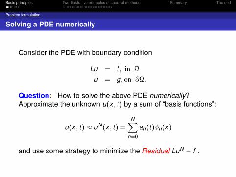
Solving a PDE numerically

Consider the PDE with boundary condition

Lu = f , in Ω

u = g, on ∂Ω.

Question: How to solve the above PDE numerically?Approximate the unknown u(x , t) by a sum of “basis functions”:

u(x , t) ≈ uN(x , t) =N∑

n=0

an(t)φn(x)

and use some strategy to minimize the Residual LuN − f .


Problem formulation

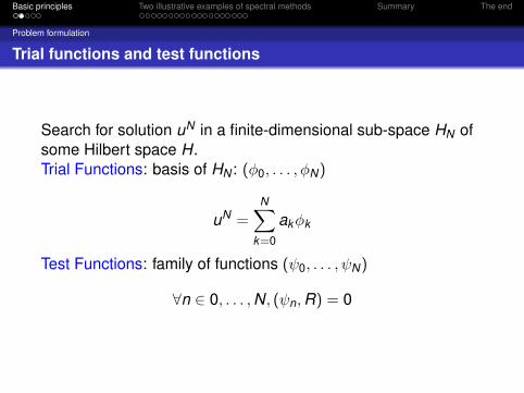
Trial functions and test functions

Search for solution uN in a finite-dimensional sub-space HN ofsome Hilbert space H.Trial Functions: basis of HN : (φ0, . . . , φN)

uN =N∑

k=0

akφk

Test Functions: family of functions (ψ0, . . . , ψN)

∀n ∈ 0, . . . ,N, (ψn,R) = 0


Various numerical methods

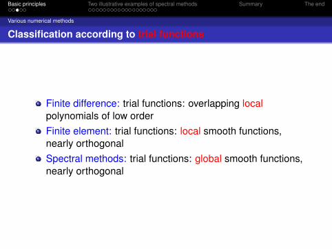
Classification according to trial functions

Finite difference: trial functions: overlapping localpolynomials of low orderFinite element: trial functions: local smooth functions,nearly orthogonalSpectral methods: trial functions: global smooth functions,nearly orthogonal


Various spectral methods

Classification according to test functions

Galerkin: ψn = φn, φn satisfy some or all of the boundaryconditions.Collocation: ψn = δ(x − xn), xn are collocation points.Tau: ψn = φn, but φn do not satisfy the boundaryconditions.


How to choose trial functions

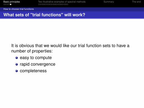
What sets of "trial functions" will work?

It is obvious that we would like our trial function sets to have anumber of properties:

easy to computerapid convergencecompleteness


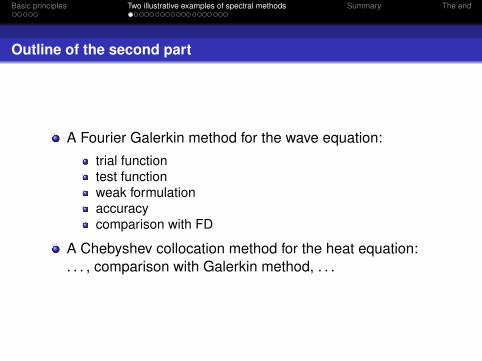
Outline of the second part

A Fourier Galerkin method for the wave equation:

trial functiontest functionweak formulationaccuracycomparison with FD

A Chebyshev collocation method for the heat equation:. . . , comparison with Galerkin method, . . .


A Fourier Galerkin method for the wave equation

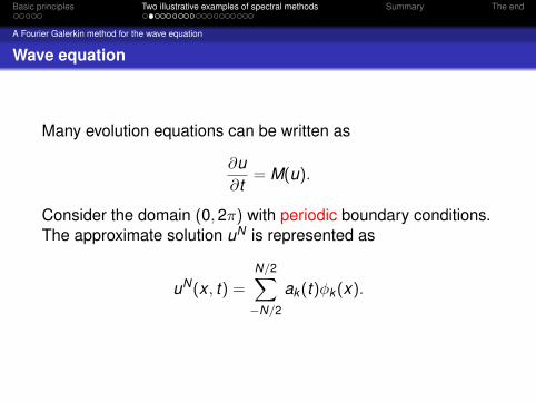
Wave equation

Many evolution equations can be written as

∂u∂t

= M(u).

Consider the domain (0,2π) with periodic boundary conditions.The approximate solution uN is represented as

uN(x , t) =

N/2∑−N/2

ak (t)φk (x).



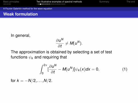
Weak formulation

In general,∂uN

∂t6= M(uN).

The approximation is obtained by selecting a set of testfunctions ψk and requiring that∫ 2π

0[∂uN

∂t−M(uN)]ψk (x)dx = 0, (1)

for k = −N/2,. . . ,N/2.



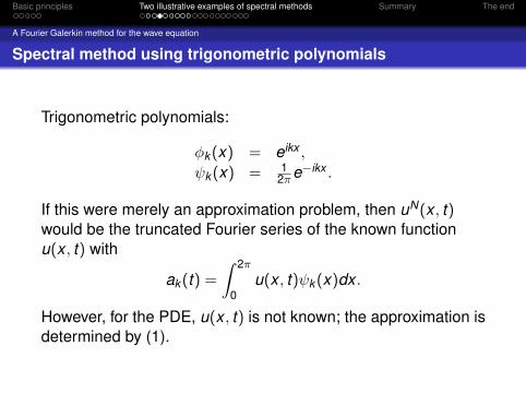
Spectral method using trigonometric polynomials

Trigonometric polynomials:

φk (x) = eikx ,

ψk (x) = 12πe−ikx .

If this were merely an approximation problem, then uN(x , t)would be the truncated Fourier series of the known functionu(x , t) with

ak (t) =

∫ 2π

0u(x , t)ψk (x)dx .

However, for the PDE, u(x , t) is not known; the approximation isdetermined by (1).



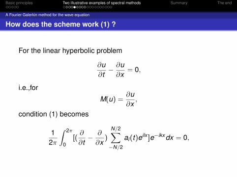
How does the scheme work (1) ?

For the linear hyperbolic problem

∂u∂t− ∂u∂x

= 0,

i.e.,for

M(u) =∂u∂x,

condition (1) becomes

12π

∫ 2π

0[(∂

∂t− ∂

∂x)

N/2∑−N/2

al(t)eilx ]e−ikxdx = 0,



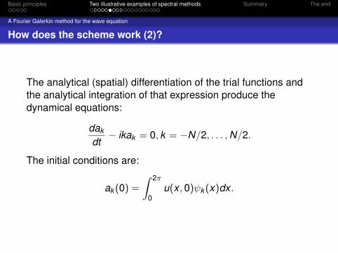
How does the scheme work (2)?

The analytical (spatial) differentiation of the trial functions andthe analytical integration of that expression produce thedynamical equations:

dak

dt− ikak = 0, k = −N/2, . . . ,N/2.

The initial conditions are:

ak (0) =

∫ 2π

0u(x ,0)ψk (x)dx .



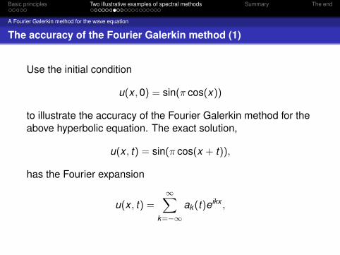
The accuracy of the Fourier Galerkin method (1)

Use the initial condition

u(x ,0) = sin(π cos(x))

to illustrate the accuracy of the Fourier Galerkin method for theabove hyperbolic equation. The exact solution,

u(x , t) = sin(π cos(x + t)),

has the Fourier expansion

u(x , t) =∞∑

k=−∞ak (t)eikx ,



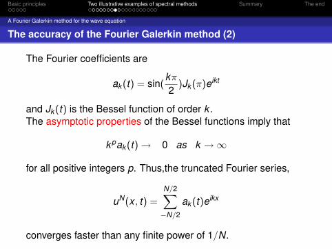
The accuracy of the Fourier Galerkin method (2)

The Fourier coefficients are

ak (t) = sin(kπ2

)Jk (π)eikt

and Jk (t) is the Bessel function of order k .The asymptotic properties of the Bessel functions imply that

kpak (t)→ 0 as k →∞

for all positive integers p. Thus,the truncated Fourier series,

uN(x , t) =

N/2∑−N/2

ak (t)eikx

converges faster than any finite power of 1/N.



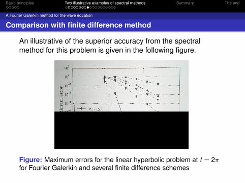
Comparison with finite difference method

An illustrative of the superior accuracy from the spectralmethod for this problem is given in the following figure.

Figure: Maximum errors for the linear hyperbolic problem at t = 2πfor Fourier Galerkin and several finite difference schemes


A Chebyshev collocation method for the heat equation

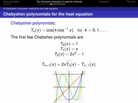
Chebyshev polynomials for the heat equation

Chebyshev polynomials:

Tk (x) = cos(k cos−1 x), for k = 0,1, . . . .

The first few Chebshev polynomials are

T0(x) = 1T1(x) = x

T2(x) = 2x2 − 1. . .

Tn+1(x) = 2xTn(x)− Tn−1(x).



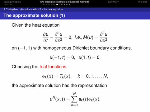
The approximate solution (1)

Given the heat equation

∂u∂t− ∂2u∂x2 = 0, i .e.,M(u) =

∂2u∂x2

on (−1,1) with homogeneous Dirichlet boundary conditions,

u(−1, t) = 0, u(1, t) = 0.

Choosing the trial functions

φk (x) = Tk (x), k = 0,1, . . . ,N,

the approximate solution has the representation

uN(x , t) =N∑

k=0

ak (t)φk (x).



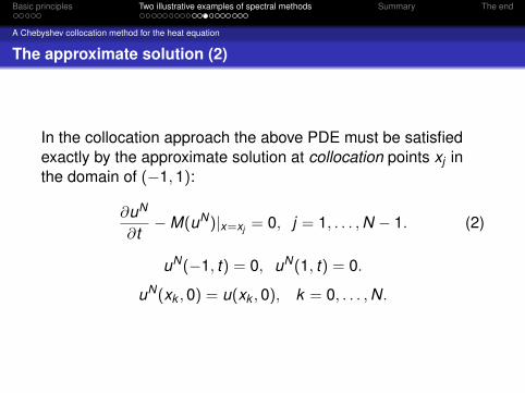
The approximate solution (2)

In the collocation approach the above PDE must be satisfiedexactly by the approximate solution at collocation points xj inthe domain of (−1,1):

∂uN

∂t−M(uN)|x=xj = 0, j = 1, . . . ,N − 1. (2)

uN(−1, t) = 0, uN(1, t) = 0.

uN(xk ,0) = u(xk ,0), k = 0, . . . ,N.



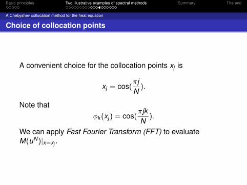
Choice of collocation points

A convenient choice for the collocation points xj is

xj = cos(πjN

).

Note thatφk (xj) = cos(

πjkN

).

We can apply Fast Fourier Transform (FFT) to evaluateM(uN)|x=xj .



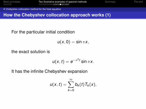
How the Chebyshev collocation approach works (1)

For the particular initial condition

u(x ,0) = sinπx ,

the exact solution is

u(x , t) = e−π2t sinπx .

It has the infinite Chebyshev expansion

u(x , t) =∞∑

k=0

bk (t)Tk (x),




. . . wherebk (t) =

2ck

sin(kπ2

)Jk (π)e−π2t

with

ck =

2, k = 0,1, k ≥ 1

Since Jk (π) is decaying rapidly, the truncated series convergesat an exponential rate. A well-designed collocation method willdo the same.




A collocation method is implemented in terms of the nodalvalues uj(t) = uN(xj , t) and we have the expansion

uN(x , t) =N∑

j=0

uj(t)φj(x),

and now φj denote the characteristic Lagrange polynomialswith the property φj(xi) = δij for 0 ≤ i , j ≤ N. The expansioncoefficients are given by

ak (t) =2

Nck

N∑l=0

c l−1ul(t) cos

πlkN, k = 0,1, . . . ,N,

where

ck =

2, k = 0 or N1, 1 ≤ k ≤ N − 1




The exact derivative of uN(x , t) becomes

∂2uN

∂x2 (t) =N∑

k=0

a(2)k (t)Tk (x),

where

a(1)N+1(t) = 0, a(1)

N (t) = 0,cka(1)

k (t) = a(1)k+2(t) + 2(k + 1)ak+1(t), k = N − 1, . . . ,0,

and

a(2)N+1(t) = 0, a(2)

N (t) = 0,cka(2)

k (t) = a(2)k+2(t) + 2(k + 1)a(1)

k+1(t), k = N − 1, . . . ,0.




The coefficients a(2)k depend linearly on the nodal values ul ;

thus, there exists a matrix D2N such that

∂2uN

∂x2 (t)|x=xj =N∑

k=0

a(2)k (t) cos

πjkN

=N∑

l=0

(D2N)jlul(t).

Substituting the above expression into (2), we obtain a systemof ODE for the nodal unknowns:

duj

dt(t) =

N∑l=0

(D2N)jlul(t), j = 1, . . . ,N − 1.

Supplemented by the initial conditions, the ODE system for thenodal values of solution is readily integrated in time.



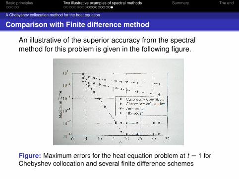
Comparison with Finite difference method

An illustrative of the superior accuracy from the spectralmethod for this problem is given in the following figure.

Figure: Maximum errors for the heat equation problem at t = 1 forChebyshev collocation and several finite difference schemes


Pros and Cons of spectral methods

Spectral methods have many advantages over FD and FEmethods:

high accuracyefficiencyexponential convergency/spectral convergency

However, spectral methods also suffers drawbacks in thefollowing folds:

coding: more difficult to code than FDcost: costly per degree of freedom than FDgeometry: for complicated domains, heavy loss ofaccuracy


Thanks for your attention!

spectral methods

Documents