Speckle Filtering of SAR Images - A Comparative Study

Between Complex-Wavelet-Based and Standard Filters �

L. Gagnon and A. Jouan

D�epartement de R&D, Lockheed Martin Canada, 6111 Ave. Royalmount, Montr�eal(Qu�ebec), H4P 1K6, CANADA

ABSTRACT

We present a comparative study between a complexWavelet Coe�cient Shrinkage (WCS) �lter and several standard speckle�lters that are widely used in the radar imaging community (Lee, Kuan, Frost, Geometric, Kalman, Gamma, etc.). The WCS�lter is based on the use of Symmetric Daubechies (SD) wavelets which share the same properties as the real Daubechieswavelets but with an additional symmetry property. The �ltering operation is an elliptical soft-thresholding procedure withrespect to the principal axes of the 2-D complex wavelet coe�cient distributions. Both qualitative and quantitative results(signal to mean square error ratio, equivalent number of looks, edgemap �gure of merit) are reported. Tests have beenperformed using simulated speckle noise as well as real radar images. It is found that the WCS �lter performs equally well asthe standard �lters for low-level noise and slightly outperforms them for higher-level noise.

Keywords: Image processing, Synthetic Aperture Radar, Speckle, Wavelets

1. INTRODUCTION

The aim of this paper is to present the results of a comparative study between a complex Wavelet Coe�cientShrinkage (WCS) �lter and several custom speckle �lters that are largely used by Synthetic Aperture Radar (SAR)imaging scientists. Our WCS �lter is based on the use of Symmetric Daubechies (SD) wavelets, which are obtainedfrom a complex multiresolution analysis (MRA).

The present work is part of the image analysis activities at Lockheed Martin Canada (LM Canada). The companyis the prime contractor for a new Spotlight SAR (SSAR) sensor and is involved in the study, design, implementationand development of algorithms for airborne surveillance applications. In particular, these include the study ofalgorithms for the fusion of dissimilar data coming from imaging (SAR, FLIR) and non-imaging sensors (radar,ESM, IFF,...) in order to (1) improve long range Automatic Target Recognition (ATR) (especially ship targets) and(2) enhance Command & Control Systems1.

1.1 Speckle

Speckle noise is a common phenomena in all coherent imaging systems like laser, acoustic and SAR imagery2�4.The source of this noise is attributed to random interference between the coherent returnsy issued from the numerousscatterers present on a surface, on the scale of a wavelength of the incident radar wave (i.e. a resolution cell). Specklenoise is often an undesirable e�ect, especially for ATR systems. Thus, speckle �ltering turns out to be a criticalpre-processing step for detection/classi�cation optimisation.

Basically, SAR speckle reduction techniques fall into two categories: non-coherent (or multi-look integration)and adaptive image restoration techniques (post-image formation methods). Multi-look techniques5 consist of (1)dividing the bandwidth of the azimuth (along track) spectrum of the radar image into L segments (called looksand corresponding to L echo spectra of the same scene point generated by L incident radar pulses), (2) forming L

�SPIE Proc. #3169, conference "Wavelet Applications in Signal and Image Processing V", San Diego, 1997yEarly descriptions of speckle noise were given by optical scientists around 1962. They used to use the term \wavelets" rather than

\returns", in reference to the historical Huyghens's nomenclature for the description of light propagation and di�usion.

independent images from these spectra and (3) incoherently averaging them. This reduces the azimuth spectrumbandwidth, and thus speckle noise, but at the expense of increasing the computational load and degrading the imageresolution if L is too large. However, many SAR systems integrate few looks during the image formation in orderto minimally improve image quality. If necessary, residual speckle has to be processed using post-image formation�lters6�14. Among the more widely used �lters are the Median, Lee, Kuan, Frost and Gamma �lters. Others likethe Kalman, Geometric, Oddy and AFS �lters are less common (maybe because of the algorithmic complexity)but are nevertheless considered as competitive candidates to the \standard" �lters. All these �lters usually performe�ciently on most SAR images but with some limitations regarding resolution degradation and smoothing of uniformareas. Wavelet-based �lterings have been proposed to overcome these di�culties15�19. They are essentially based ona WCS approach and seem to demonstrate a higher quality in image enhancement (i.e. good signal averaging overhomogeneous regions with minimal resolution degradation of image details). We have recently proposed such a �lter,based on the use of SD wavelets19. The performance results were encouraging but comparative tests were performedonly with a small subset of standard �lters (Median and Geometric). A more extensive test bank was required inorder to better validate our tool; this is the purpose of the present work.

1.2 Speckle statistics

Fully developed speckle (i.e. when the number of scatterers is large in one resolution cell) has the characteristics ofa random multiplicative noise. Under the assumption that the real and imaginary parts (respectively the so-called in-phase (denoted I) and quadrature (denoted Q) components of a complex radar image) of the speckle have zero-meanGaussian density, noise intensity can be shown to follow a Gamma distribution (which reduces to an exponentialdistribution for single-look images)5. The mean-to-standard-deviation ratio (a measure of the signal-to-noise ratio)of such a distribution satis�es � mean

standard deviation

�2= L = constant (1:1)

A usual way to estimate the speckle noise level in a SAR image is to calculate Eq. (1.1), often termed the EquivalentNumber of Looks (ENL), using pixel intensity values over a uniform image area. Unfortunately, the ENL carries noinformation on the resolution degradation and because of that, we will use it jointly with the Signal-to-Mean-Square-Error Ratio (S/MSE) (10log10[

Ppixels I

21=P

pixels(I2 � I1)2], where I1 and I2 are the unnoisy and noisy images,

respectively) which corresponds to the standard SNR in case of additive noise.

Experimentally measured speckle distributions can deviate from the theoretical Gamma distribution for speci�ctypes of targets. For instance, Log-Normal distribution turns out to be a good speckle model for high-resolutionsea-clutter imagery20. Because of our particular interest in ocean surveillance, we have retained this distribution inour speckle simulations. However, it appeared later that this choice is not critical (tests performed with the Gammadistribution have shown no signi�cant change in the �lter performance results). One can generate the Log-Normaldistribution using

XLog�Normal = exp(XNormal

p2 logM=m+ lnm) (1:2)

where M and m are the mean and median values of the distribution and XNormal � N(0; 1). Without loss ofgenerality, we have chosen M = 1. The equivalence between m and L has been calculated numerically and is givenin Table 1.

m 0.70 0.75 0.80 0.85 0.87 0.90 0.92 0.95 0.97 0.99L 1.0 1.4 1.9 2.7 3.2 4.4 5.6 9.4 16 50

Table 1: Number of looks L as a function of median parameter m for the Log-Normal distribution (1.2) with M = 1

1.3 Symmetric Daubechies wavelets

Symmetric Daubechies (SD) wavelets, and their underlying scaling functions, are obtained from a complexMRA21;22. The complex scaling function '(x) and wavelet (x) satisfy the usual MRA equations

'(x) = 2Xk

ak '(2x� k) (x) = 2Xk

bk '(2x� k) (1:3)

withak = a2J+1�k; bk = (�1)ka?2J+1�k J = 0; 2; 4; 6; ::: k = 0; :::; 2J + 1 (1:4)

where ? stands for complex conjugate.

In addition to sharing the same properties as the real Daubechies wavelets (i.e. compact support, orthogonalityand vanishing moments), SD wavelets and scaling functions are symmetric (respectively of odd and even parity withrespect to the center of the compact support) and have a better interpolation capability due to identical vanishingof the second centered moment of the real part of the scaling function23. Multiwavelets can also hold concurrentlyall these properties24 and in fact, as is obvious from Eq. (1.3), SD wavelets also have a multi-wavelet interpretationin terms of 2x2 matrices.

Symmetry is the property that makes SD wavelets particularly interesting for image processing applications. Itallows the use of symmetric extension of data at the image boundaries. Symmetric extension prevents discontinuitiesintroduced by a periodic wrapping of the data. Apart from slightly increasing the computational load, the complex-value of the transform is not really a drawback (Fourier transform is also complex!). Like Fourier, SD waveletsintroduce redundancy in the transformation of a real signal but this can be used in an advantageous way for the designof local multiresolution sharpening operators and POCS (Projection Onto Convex Sets) �ltering algorithms23;25.Also, it has been experimentally demonstrated that phase of the wavelet coe�cients encodes much information onedges25.

2. SPECKLE FILTERS

2.1 Wavelet �lter

Our wavelet speckle �lter is based on the well-known soft-thresholding procedure26. However, use of SD waveletsprovides an opportunity to modify this algorithm in order to manage the complex-valued characteristic.

We have numerically observed that wavelet coe�cients in each spectral band (the so-called VW, WV and WWblocks) can be modelized as a bi-Normal distribution of mean (�x; �y) (nearly zero) and covariance matrix R which isin general not diagonal (real and imaginary parts are correlated). In addition, the distributions are usually orienteddi�erently in each block (Figure 1). Based on this fact, it seemed natural to us to propose an algorithm that performswavelet coe�cients thresholding with respect to the principal axes (�; �) of the 2-D distributions. As a result, thethreshold level becomes angle-dependent and extends in proportion to the eccentricity of the centered dispersionellipse. In practice, since the noise characteristics can di�er in each block, we have also chosen to process themseparately. Thus, the VW block at the highest resolution level provides noise statistics for thresholding all the lowerresolution VW blocks (similarly for the WV and WW blocks).

-300

-200

-100

0

100

200

300

-400 -300 -200 -100 0 100 200 300 400

ima

gin

ary

pa

rt

real part

-300

-200

-100

0

100

200

300

-400 -300 -200 -100 0 100 200 300 400

ima

gin

ary

pa

rt

real part

-300

-200

-100

0

100

200

300

-400 -300 -200 -100 0 100 200 300 400

ima

gin

ary

pa

rt

real part

Figure 1: Illustration of the elliptical thresholding rule on a complex wavelet coe�cient distribution.Left: before thresholding. Center: elliptical thresholding area. Right: after thresholding

The complete WCS for SAR image then proceeds as follows19.

� Make a logarithmic transformation (more precisely log(I + 1:0)) of the original image I

� Make a N-level SD wavelet transform

� For each block type (VW, WV and WW) and level j (j=1,2,...,N), perform the following operations:

{ Calculate the mean, covariance matrix elements, orientation angle and uncorrelated standard deviations�� and �� of the wavelet coe�cient distribution

{ Noting wk � � + i� (with respect to the principal axis coordinates), apply the following elliptical soft-thresholding rule

jwk j ! 0 if�2

t2�+�2

t2�� 1:0 jwkj ! jwkj � T (�) if

�2

t2�+�2

t2�> 1:0 (2:1)

where

T (�) =t�t�p

(t� sin �)2 + (t� cos �)2; t� = ��1� t� = t���=�� (2:2)

� is the phase of the wavelet coe�cient distribution (with respect to the principal axes), �1� is the principalstandard deviation along the �-axis at the �nest resolution level and � is a free denoising parameter.

� Invert the DWT

� Invert the logarithmic transformation

8

8.5

9

9.5

10

10.5

11

S/M

SE

Threshold

Figure 2: Variation of the S/MSE as function of � and for N = 1; :::; 6 (see text for details)

The logarithm transformation is a common homomorphic transformation performed on SAR images and is usedto transform multiplicative noise into additive noise3. It also allows compliance with the additive noise hypothesisin the standard WCS algorithm26.

In order to minimize the image artifacts (Gibbs-like phenomena) resulting from the lack of translation invarianceof discrete wavelet bases, we have embeded our algorithm into the cycle spinning algorithm27. This consists inaveraging the result of the WCS �lter over all possible shifts of the input image (16 translations were su�cient inpractice).

Most of the numerical tests have been done with the J = 2 wavelet. Its short support (6-taps) minimizes thecomputation time and no signi�cant changes are obtained with higher-order wavelets. Parameters N and � havebeen varied during the tests (1 to 6 and 0.1 to 3.0, respectively) in order to have a clear picture of their e�ects. Intheory, N should be large but in practice we have limited the number of decomposition levels to 6. Figure 2 showsthe SMSER obtained after processing an urban image corrupted by a simulated 4.4 dB Log-Normal noise (L = 2:7).Each curve corresponds to a di�erent value of N (1 to 6). Upper curves (diamonds) are for SD wavelets while lowerones (crosses) are for the 6-taps real Daubechies wavelet (with periodic warping of boundary data). Points on eachcurve are for di�erent values of �. In this case, an optimal S/MSE is obtained for N = 6 and � = 1:4. All thecomparative results presented in the next section are for optimal S/MSE values only.

2.2 Standard �lters

Let x be an image pixel corrupted by a stationary multiplicative noise n such that y = nx. Without loss ofgenerality, we assume noise of unit-mean (�n = 1). Many standard �lters require knowledge of �y as well as thestandard deviations �y and �n. In practice, �y and �y are estimated locally, within a �nite size window. Noisestandard deviation �n (and L) is given as an input �lter parameter or can be estimated over a uniform area in theimage. In fact, under the unit-mean noise assumption, we have ENL = (�y=�y)

2 = 1=�2n.

The 8 standard speckle �lters considered in this comparative study are the following.

Kuan �lter

The Kuan �lter is based on a Minimum Mean Square Error (MMSE) criterion8. A MMSE estimate is �rstdeveloped for and additive noise model y = x+n. The multiplicative noise model is then considered under the formy = x + (n � 1)x from which the corresponding linear �lter is deduced. The Kuan �lter is optimal when both thescene and the detected intensities are Gaussian distributed. Under the unit-mean noise assumption, the pixel valueestimate x̂ is given by

x̂ = �y +�2x(y � �y)

�2x + (�y2 + �2x)=L�2x =

L�2y � �y2

L+ 1(2:3a; b)

We have put x̂ = �y for the pathological cases where measures yield �2x < 0.

Lee �lter

The Lee �lter (more precisely Lee MMSE �lter6) is a particular case of the Kuan �lter when the term �2x=L isremoved in Eq. (2.3a). This term does not appear in Lee's original derivation due to a linear approximation madethere for the multiplicative noise model (a �rst-order Taylor series expansion of y about x and n).

Another �lter that is a particular case of Kuan is the Nathan �lter9. This one is obtained by puting L = 1 in Eq.(2.3) and is thus applicable to 1-look SAR images only. For this reason, it has not been included in our tests.

Gamma �lter

The Gamma �lter is a Maximum A Posteriori (MAP) �lter based on a Bayesian analysis of the image statistics13.It assumes that both the radar re ectivity and the speckle noise follow a Gamma distribution. The \superposition"of these distributions yields a K-distribution which is recognized to match a large variety of radar return distributionsof land and ocean targets. The estimate x̂ is given by

x̂ =(�� L� 1)�y +

p�y2(�� L� 1)2 + 4�Ly�y

2�� =

L+ 1

L(�y=�y)2 � 1(2:4)

We have put x̂ = �y for the pathological cases where measures yield a negative or a complex estimate for x̂.

Frost �lter

The Frost �lter7 is an adaptive Wiener �lter which convolves the pixel values within a �xed size window with anexponential impulse response m given by

m = exp[�KCy(t0)jtj] Cy = �y=�y (2:5)

where K is the �lter parameter, t0 represents the location of the processed pixel and jtj is the distance measuredfrom pixel t0. This response results from an autoregressive exponential model assumed for the scene re ectivity x.

Kalman �lter

A 2D Kalman �lter has been implemented on a causal prediction window, the so-called Non-Symmetric HalfPlane (NSHP), de�ned as W = fp; q : 1 � p �M;�M � q �M ; p = 0; 1 � q �Mg, with M = 2. In this �lter, theimage is assumed to be represented by a Markov �eld which satis�es the causal autoregressive (AR) model

x(m;n) =X

(p;q)2W

apqx(m� p; n� q) + u(m;n) (2:6)

where x(m;n) represents the pixel value at location (m;n), u(m;n) is a noise sequence (this is not the speckle noise)which drives the Markov process and apq are the re ection coe�cients of the AR model. The parameters apq areevaluated based upon the global estimates of the autocorrelation sequence of the image over the �nite window W .From these parameters, the AR model can be arranged into a 2D block recursive form (Figure 3) for the Kalman�lter equations. Implementation of this �lter is very much involved and we refer to Ref. 14 for more details aboutthe 2D kinematic model (limited here to speckle modelling only) and the Kalman �lter equations.

Geometric �lter

The geometric �lter is a nonlinear morphological �lter that uses the concept of image graph12. The image graphis obtained by transforming the original image into a 3-dimensional diagram where the pixel coordinates specify theposition of the pixel on a plane and the pixel value speci�es the elevation of the pixel with respect to that plane. The�ltering process itself is performed �rst on row slices (i.e. 1-dimensional pro�le graphs similar to Figure 4a) of theimage graph using a 8-hulling algorithm. Slice pixels are set to 1 if the pixel is on or below the image graph surface,while pixels above the image graph surface are set to 0 (Figure 4b). The �ltering algorithm searches for 4 di�erentcon�gurations (3x3 binary morphological masks) and when it �nds one, the graph pixel corresponding to the centralpixel of the mask is set to 0. The procedure is repeated for the complementary graphs and masks (Figure 4c) exceptthat the central pixel is now incremented by 1. The whole procedure is repeated on column and diagonal slices. Thiscompletes one iterative step of the geometric �lter. A �ltering is achieved because speckle appears as narrow wallsand valleys on the binary slice images and because the geometric �lter, through iterative repetition, gradually tearsdown and �lls up these features.

Past blocks Present block

W

Image pixels(a)

(b) (c)

Figure 3 (left): 2D block recursive form for the Kalman �lterFigure 4 (center): (a) Exemple of image graph; (b) Binary slice and masks and their complements (c)

Figure 5 (right): The 8 binary masks used by the ASF �lter

Oddy �lter

The Oddy �lter can be considered as a mean �lter whose window shape varies according to the local statistics10.The estimate x̂ is given by

x̂ = �y if m < ��y; x̂ =

Pk

PlWkly(k; l)Pk

PlWkl

if m > ��y (2:7)

Wkl = 1 if jy(k; l)� yj � m; Wkl = 0 otherwise

where �x is evaluated locally over a 3x3 window, m = 1=8P

k

Pl jy(k; l)� yj and � is the �lter parameter. W plays

the role of an adaptive binary mask that is applied over the window.

AFS �lter

AFS �lter stands for Adaptive Filter on Surfaces11. It is another adaptive mask �lter that uses the concept of\local emerging surface" (l.e.s.) value. The l.e.s. is the area of the image graph surface de�ned over the window.The l.e.s. is calculated for the 9 binary masks shown in Figure 5. The mask whose l.e.s. is a minimum is selectedand a mean �ltering is performed over the mask pixels. The mean value is assigned to the central pixel of the 5x5window.

3. TESTS AND DISCUSSION

3.1 Simulated images

Figure 6: Urban test images.Upper row: original and noisy (L = 9:4). Lower row: Gamma and Wavelet �ltered (Table 2)

We have simulated radar textured images by degrading two aerial photographs (www.cent.org) with unit-meanLog-Normal multiplicative noise (Figures 6a,b and 7a,b). The two scenes (urban and agricultural regions) have

very di�erent spectral content (high and low frequency, respectively) in order to observe the e�ect on the �lters'performance. Three noise levels have been tested, corresponding to L = 2:7, 9.4 and 50. Filtering performance hasalso been calculated using measured ENL, as it is done in practical situations. A uniform area has been identi�edin each image from which ENL (or noise variance) has been measured and used in the �lter equations. Quantitativeperformance measures are summarized in Tables 2 and 3 and correspond to the best enhanced images obtained, withrespect to the S/MSE. During measures, image radiometry (image intensity) has been conserved by assuring thatthe enhanced and noisy images have the same global mean. Two of the best enhanced images for the case L = 9:4are shown on Figures 6c,d and 7c,d.

Figure 7: Agricultural test images.Upper row: original and noisy (L = 9:4). Lower row: Gamma and Wavelet �ltered (Table 3)

We observe from Tables 2 and 3 that the optimal S/MSE is highly dependent on the noise level and signal content.High spectral content images require lower wavelet coe�cient threshold values. Higher wavelet coe�cient thresholdsare necessary for higher noise levels because of the more important wavelet coe�cient distribution spreading.

Quantitatively, the WCS �lter performs as well as the best standard �lters (Frost, Gamma, Kuan) for low-levelspeckle noise (L > 10) and slightly outperforms them for higher speckle noise level (L < 10), especially in the case oflow spectral content (Figure 7). This is veri�ed for speci�c wavelet �lter parameter values. Qualitatively, the wavelet�lter o�ers the best trade-o� between image resolution conservation and averaging over uniform regions. This can be

L = 2:7 L = 9:4 L = 50S/MSE ENL Notes S/MSE ENL Notes S/MSE ENL Notes(dB) (dB) (dB)

Noisy 4.4 9.8 17.0

Lee 9.0 144 5x5 12.8 97 3x3 18.5 446 3x3Kuan 9.4 144 5x5 13.0 97 3x3 18.5 448 3x3Gamma 9.6 140 5x5 13.1 96 3x3 18.6 448 3x3Frost 10.2 127 7x7; K1:5 13.4 84 3x3; K3:0 18.7 386 3x3; K7:0

Kalman - - 11.7 39 - -Geometric 7.9 144 3 iter. 11.6 93 2 iter. 17.5 206 1 iter.Oddy 10.0 47 5x5; �0:7 12.9 110 3x3; �0:5 16.6 367 3x3; �0:2AFS 8.3 37 9.4 86 10.7 433

Wavelet 10.9 151 N6; �1:4 13.6 172 N6; �0:8 18.6 340 N6; �0:3

Table 2: Quantitative enhancement measures performed on the urban test image (Figure 6)

L = 2:7 L = 9:4 L = 50S/MSE ENL Notes S/MSE ENL Notes S/MSE ENL Notes(dB) (dB) (dB)

Noisy 4.3 9.7 17.0

Lee 13.6 68 7x7 17.3 129 7x7 21.9 310 7x7Kuan 14.0 74 7x7 17.4 140 7x7 21.9 319 7x7Gamma 14.1 80 7x7 17.5 146 7x7 22.0 373 7x7Frost 14.6 156 7x7; K1:0 17.4 155 7x7; K3:0 22.1 313 7x7; K7:0

Kalman - - 15.8 63 - -Geometric 13.8 471 4 iter. 16.1 555 3 iter. 20.8 218 1 iterOddy 14.3 89 7x7; �0:8 16.9 146 7x7; �0:5 20.6 370 3x3; �0:3AFS 12.2 29 14.8 90 17.2 270

Wavelet 16.3 241 N6; �2:0 18.6 345 N6; �1:6 22.1 427 N6; �0:8

Table 3: Quantitative enhancement measures performed on the agricultural test image (Figure 7)

observed, in particular, on the enhanced urban images (Figure 6). This also happens to be observed in the followingexperiment about edge preservation measure.

3.2 Edge map

An edge map is a binary image identifying pixels that are on an edge. In order to get a quantitative evaluation ofedge preservation for each �lter, we have performed an experiment proposed by Frost et al.7. The following procedurehas been used to create an edge map under a controlled environment (1) simulate an arti�cial noisy edge (a 200-50pixel intensity step here), (2) apply the �lter, (3) apply a Robert's gradient operator for edge detection, (4) create abinary image by thresholding the pixel values and (4) calculate an edge map Figure Of Merit (FOM).

The edge FOM used here is the one proposed by Abdou and Pratt28. Let two congruent images I and A, representideal and actual edge maps of a single step edge. The ideal edge map is assumed to contain NI edge pixels, whilethe actual edge map contains NA. If d is the perpendicular distance from the actual edge pixel to the ideal edge, onecan de�ne a FOM by

R(%) =100

max(NA; NI)

NAXi=1

1

1 + �d2(3:1)

where � is an arbitrary penalty parameter for o�set edge pixels (we choose � = 10 here). A perfect edge map yieldsR = 100%. Since the selection of the threshold greatly a�ects the nature of the edge map, the threshold that yields

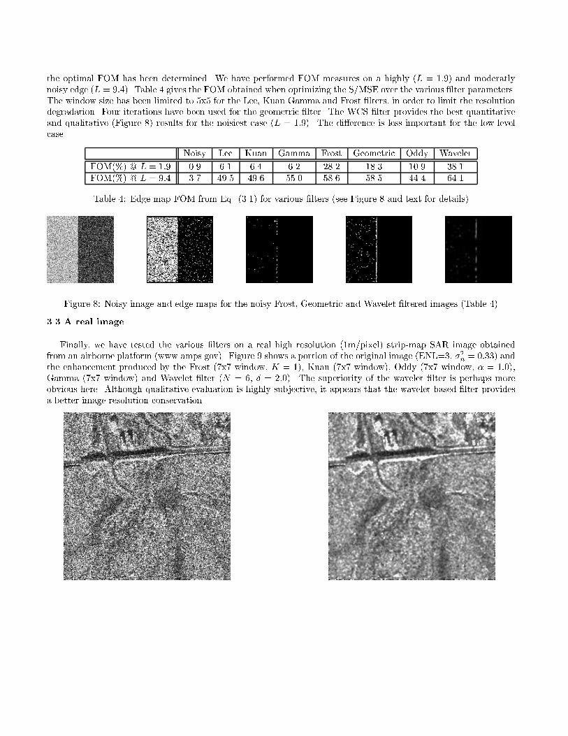
the optimal FOM has been determined. We have performed FOM measures on a highly (L = 1:9) and moderatlynoisy edge (L = 9:4). Table 4 gives the FOM obtained when optimizing the S/MSE over the various �lter parameters.The window size has been limited to 5x5 for the Lee, Kuan Gamma and Frost �lters, in order to limit the resolutiondegradation. Four iterations have been used for the geometric �lter. The WCS �lter provides the best quantitativeand qualitative (Figure 8) results for the noisiest case (L = 1:9). The di�erence is less important for the low-levelcase.

Noisy Lee Kuan Gamma Frost Geometric Oddy Wavelet

FOM(%) @ L = 1:9 0.9 6.1 6.4 6.2 28.2 18.3 10.9 38.1FOM(%) @ L = 9:4 3.7 49.5 49.6 55.0 58.6 58.5 44.4 64.1

Table 4: Edge map FOM from Eq. (3.1) for various �lters (see Figure 8 and text for details)

Figure 8: Noisy image and edge maps for the noisy Frost, Geometric and Wavelet �ltered images (Table 4)

3.3 A real image

Finally, we have tested the various �lters on a real high resolution (1m/pixel) strip-map SAR image obtainedfrom an airborne platform (www.amps.gov). Figure 9 shows a portion of the original image (ENL=3, �2n = 0:33) andthe enhancement produced by the Frost (7x7 window, K = 1), Kuan (7x7 window), Oddy (7x7 window, � = 1:0),Gamma (7x7 window) and Wavelet �lter (N = 6, � = 2:0). The superiority of the wavelet �lter is perhaps moreobvious here. Although qualitative evaluation is highly subjective, it appears that the wavelet-based �lter providesa better image resolution conservation.

Figure 9: Noisy, Frost, Kuan, Oddy, Gamma and Wavelet enhancement for a real SAR image

4. CONCLUSIONS

We have presented a comparative study between a complex Wavelet Coe�cient Shrinkage (WCS) �lter and severalstandard speckle �lters that are widely used in the radar imaging community (Lee, Kuan, Frost, Geometric, Kalman,Gamma, etc.). The WCS �lter is based on the use of Symmetric Daubechies (SD) wavelets. There are two advantagesin using SD wavelets: (1) symmetric extension prevents discontinuities introduced by a periodic wrapping of the dataand (2) identical vanishing of the second centered moment of the real part of the scaling function provides betterapproximation at sampling points.

Our comparative tests with 8 standard speckle �lters have shown that our WCS wavelet-based �lter is amongthe best speckle �lters. This �lter quantitatively performs equally well for low-level noise (L > 10) and slightlyoutperforms standard ones (Lee, Kuan, Frost, Gamma, etc.) for higher speckle noise level (L < 10). Up to 10%improvement has been measured on a low spectral content image. The current drawback is that computational loadmight necessitate specialized hardware for real-time applications; processing of a 512x512 images takes about 3 min.on a Pentium 90 (the size of strip-map mode SAR images can easily exceed 4000x4000 pixels). Also, in practice, thetheoretical threshold for wavelet coe�cient shrinkage does not necessarily lead to the optimal signal-to-noise ratiofor the enhanced image. A robust threshold estimator is still needed in order to automate the �ltering process.

5. REFERENCES

[1] E. Shahbazian, L. Gagnon, J.-R. Duquet, M. Macieszczak, P. Valin, \Fusion of Imaging and Non-Imaging Data for

Surveillance Aircraft", SPIE Proc. #3067, 1997

[2] J. W. Goodman, \Some Fundamental Properties of Speckle", J. Opt. Soc. Am., Vol. 66, pp. 1145-1150, 1976

[3] H. H. Arsenault, G. April, \Properties of Speckle Integrated with a Finite Aperture and Logarithmically Transformed",

J. Opt. Soc. Am., Vol. 66, pp. 1160-1163, 1976

[4] J. S. Lim, H. Nawab, \Techniques for Speckle Noise Removal", Opt. Engineering, Vol. 20, pp. 472-480, 1981

[5] D. R. Wehner, High-Resolution Radar, 2nd edition (Artech House, Boston, 1994)

[6] J.-S. Lee, \Digital Image Enhancement and Noise Filtering by Use of Local Statistics", IEEE Transactions on Pattern

Analysis and Machine Intelligence, Vol. PAMI-2, pp. 165-168, 1980

[7] V. S. Frost, J. A. Stiles, K. S. Shanmugan, J. C. Holtzman, \A Model for Radar Images and Its Application to Adaptive

Digital Filtering of Multiplicative Noise", IEEE Transactions on Pattern Analysis and Machine Intelligence, Vol. PAMI-4, pp.

157-166, 1982

[8] D. T. Kuan, A. A. Sawchuk, T. C. Strand, P. Chavel, \Adaptive Noise Smoothing Filter for Images with Signal-

Dependent Noise", IEEE Transactions on Pattern Analysis and Machine Intelligence, Vol. PAMI-7, pp. 165-177, 1985

[9] K. S. Nathan and J. C. Curlander, \Speckle Noise Reduction of 1-Look SAR Imagery", Proc. IGARSS '87 Symposium,

pp. 1457-1462, 1987

[10] C. J. Oddy, A. J. Rye, \Segmentation of SAR Images using a Local Similarity Rule", Pattern Recognition Letters,

Vol. 1, pp. 443-449, 1983

[11] L. Alparone, F. Boragine, S. Fini, \Parallel Architectures for the PostProcessing of SAR Images", SPIE Proc. #1360,

pp. 790-802, 1990

[12] T. R. Crimmins, \Geometric Filter for Speckle Reduction", Appl. Optics, Vol. 24, pp. 1438-1443, 1985

[13] A. Lopes, E. Nezry, R. Touzi, H. Laur, \Structure Detection and Statiscal Adaptive Speckle Filtering in SAR Images",

Int. J. Remote Sensing, Vol. 14, pp. 1735-1758, 1993

[14] M. R. Azimi-Sadjadi, S. Bannour, \Two-Dimensional Adaptive Block Kalman Filtering of SAR Imagery", IEEE Trans.

Geosci. and Remote Sensing, Vol. 29, pp. 742-753, 1991

[15] T. Ranchin, F. Cauneau, \Speckle Reduction in Synthetic Aperture Radar Imagery Using Wavelets", SPIE Proc.

#2034, pp. 432-441, 1993

[16] J. E. Odegard, H. Guo, M. Lang, C. S. Burrus, R. O. Wells Jr., L. M. Novak, M. Hiett, \Wavelet Based SAR Speckle

Reduction and Image Compression", SPIE Proc. #2487, pp. 259-271, 1995

[17] H. Guo, J. E. Odegard, M. Lang, R. A. Gopinath, I. W. Selesnick and C. S. Burrus,\Wavelet Based Speckle Reduction

with Application to SAR Based ATD/R", IEEE Proceedings of ICIP '94, pp. 75-79, 1994

[18] K. Lebart, J.-M. Boucher, \Speckle Filtering by Wavelet Analysis and Synthesis", SPIE Proc. #2825, 644-651 (1996)

[19] L. Gagnon, F. Drissi Smaili, \Speckle Noise Reduction of Airborne SAR Images with Symmetric Daubechies Wavelets",

SPIE Proc. #2759, pp. 14-24, 1996

[20] H.-C. Shyu, Y.-S. Sun and W.-H. Shen, \The Analysis of Scan-to-Scan Integration Techniques for Sea Clutter", IEEE

Proc. Nat. Radar Conf., pp. 228-233, 1994

[21] W. Lawton, \Application of Complex Valued Wavelet Transforms to Subband Decomposition", IEEE Trans. Signal

Proc., Vol. 41, pp. 3566-3568, 1993

[22] J. M. Lina and M. Mayrand, \Complex Daubechies Wavelets", App. Comp. Harmonic Anal., vol. 2, pp. 219-229,

1995

[23] J. M. Lina and L. Gagnon, \Image Enhancements with Symmetric Daubechies Wavelets", SPIE Proc. #2569, pp.

196-208, 1995

[24] V. Strela, P. N. Heller, G. Strang, P. Topiwala, C. Heil, \The Application of Multiwavelet Filter Banks to Image

Processing", submitted IEEE Trans. on Image Processing

[25] P. Drouilly, M.Sc. Thesis, D�epartement de Physique, Univ. de Montr�eal, 1996

[26] D. L. Donoho and I. M. Johnstone, \Adapting to Unknown Smoothness via Wavelet Shrinkage", Tech. Report #425,

Statistics Dept., Stanford Univ., 1993

[27] R. R. Coifman, D. L. Donoho, \Translation-Invariant De-Noising", in Wavelets and Statistics, Anestie Antoniadis Ed.,

Springer-Verlag Lecture Notes, 1995

[28] I. E. Abdou, W. K. Pratt, \Quantitative Design and Evaluation of Enhancement/Thresholding Edge Detectors", Proc.

IEEE, Vol. 67, pp. 753-763, 1979