Specialisation trends in the member countries of the EMU and the

effect of specialisation on the symmetry of business cycles

Master’s Thesis

Student name: Gabrielė Kusaitė

Student ID: 10630392

Supervisor: Dr D.J.M. Veestraeten

Second reader: N. J. Leefmans

Faculty: Economics and Business

Study: MSc Economics

Date: June 2017

1

Statement of Originality

This document is written by student Gabrielė Kusaitė who declares to take full responsibility for the

contents of this document. I declare that the text and the work presented in this document are original

and that no sources other than those mentioned in the text and its references have been used in creating

it. The Faculty of Economics and Business is responsible solely for the supervision of completion of the

work, not for the contents.

2

TABLE OF CONTENTS:

Abstract…………………………………………………………………………………………………………………………………………………..3

1. Introduction……………………………………………………………………………………………………………………………………..4

2. Theoretical Framework…………………………………………………………………………………………………………………….6

2.1. Theory of Optimum Currency Areas…………………………………………………………………………………………..6

2.1.1. The traditional and “new” OCA theory.………………………………………………………………………………6

2.1.2. Endogeneity of the OCA criteria………………………………………………………………………………………10

2.2. Neo-classical and “new” theories of trade and location…………………………………………………………..11

3. Empirical Findings of the Existing Research……………………………………………………………………………………13

4. Empirical Analysis of Specialisation and Business Cycle Synchronisations…………………….........………18

4.1. Empirical methodology……………………………………………………………………………………………………………18

4.1.1. The specialisation index.………………………………………………………………………………………………….18

4.1.2. Business cycles…………………………………………………………………………………………………………………19

4.1.3. Regression analysis………………………………………………………………………………………………………….20

4.2. Data…………………………………………………………………………………………………………………………………………23

4.2.1. Gross Value Added…………………………………………………………………………………………………………..23

4.2.2. Gross Domestic Product…………………………………………………………………………………………………..24

4.2.3. Additional explanatory variables………………………………………………………………………………………24

4.3. Results…………………………………………………………………………………………………………………………………….25

4.3.1. Development of specialisation indexes over time…………………………………………………………….25

4.3.2. Development of the symmetry of the business cycles over time………………………………………28

4.3.3. Regression results…………………………………………………………………………………………………………….32

5. Conclusions…………………………………………………………………………………………………………………………………….37

Bibliography…………………………………………………………………………………………………………………………………...38

Appendix…………………………………………………………………………………………………………………………………….....41

3

Abstract

This paper analyses the effects of the EMU on the specialisation and the asymmetries of the business

cycles of its members. Moreover, it examines if specialisation has had a significant effect on the

asymmetries of the business cycles within the EMU. Specialisation is measured by the specialisation index

calculated using the Gross Value Added (GVA) values. The asymmetries of the business cycles are

measured by the absolute differences between the countries’ real GDP growth rates and the average real

GDP growth rate of the EMU. The regressions are performed by employing panel data methods with both

entity and time fixed effects. The sample period of the regressions is from 1996 to 2016, while the sample

period of the specialisation index and the real GDP growth rates starts at 1995. It is found that

specialisation has on average been increasing in the EMU as a whole and in most of its members

individually after joining the EMU. The asymmetries of the business cycles have not shown a clear overall

trend and individual countries exhibit various results, including decreases and increases in asymmetry as

well as no substantial changes. Finally, specialisation was found to not have had a significant effect on the

business cycle asymmetries. Furthermore, EMU membership was shown to have had a significant negative

effect on the asymmetries, that is, membership of the EMU was found to have lowered the differences in

the GDP growth rates between the individual countries and the average of the EMU.

4

1. Introduction

The recent global financial crisis and the European debt crisis have revealed that the Economic and

Monetary Union (EMU) of the European Union (EU) has some substantial problems. A prominent example

of such problems is the situation in Greece, with the country needing several bail outs during the past

years in order to avoid default on its sovereign debt and protect national banks. In addition, it showed

that countries within the EMU still exhibit notable differences, which might imply a high probability of

asymmetric shocks. Asymmetric shocks are positive or negative economic shocks that only occur in

individual member countries or in certain regions within the EMU. They are almost impossible to handle

union-wide, given that the European Central Bank (ECB) sets a uniform monetary policy and there is no

mechanism of fiscal transfers in place. Moreover, not only do individual countries not have independent

monetary policies, but their fiscal policies are highly restricted due to the Maastricht treaty and the Fiscal

Compact as well. The inability of a country to implement monetary and/or fiscal policy on a national level

reduces its ability to tackle the consequences of asymmetric shocks. To the contrary, if shocks are

symmetric, that is, all countries in the EMU experience the same impact from the shock, monetary policy

determined by the ECB is an appropriate response for all of the EMU. Therefore, it is important to analyse

whether the issue of asymmetry is likely to create more serious problems in the future, or, possibly,

asymmetry is decreasing within the EMU.

One of the more significant factors contributing to asymmetric shocks in the economy is

specialisation of countries, as countries that are becoming increasingly specialised in certain industries

are likely to suffer more when those industries face idiosyncratic shocks. Furthermore, the likelihood of

shocks increases as well. It is important to separate two theories analysing symmetry and specialisation

in a monetary or currency union. One the one hand, the endogeneity hypothesis of the “new” theory of

Optimum Currency Areas (OCA) states that similarity of shocks or symmetry in a currency union will

increase once the monetary union is started. This will happen as a result of increased openness to trade

and a higher degree of goods market integration. On the other hand, theories of international trade

suggest that joining a monetary union will increase specialisation in the member countries. This is due to

a decrease or complete abolishment of trade barriers and a common currency within a union. Since

countries have access to a larger market and there is less uncertainty and costs involved, there is a greater

scope for exploiting economies of scale and, therefore, production becomes more spatially concentrated.

Consequently, more specialisation might lead to less symmetry in the monetary union.

It is also important to note that recently there have been several EMU enlargements, with

countries, namely Slovenia, Cyprus, Malta, Slovakia, Estonia, Latvia and Lithuania, joining the monetary

union in between 2007 and 2015. In addition to this, there is now a sufficient time span available for

studying the effects of the monetary union on the member states, considering the creation of the

Eurozone in 1999. Due to these factors and considering the relative lack of research for the most recent

years, it is worth analysing this issue.

Therefore, this paper will aim to answer the question whether joining the EMU leads to more

specialisation in member countries, and whether specialisation leads to less synchronised business cycles,

so there is a higher probability of country-specific shocks. This empirical study will be performed in three

stages. In the first stage the annual specialisation index of the EMU countries will be calculated and the

5

time trends of the index will be analysed to see whether specialisation has been increasing or decreasing

in the member states. Secondly, asymmetry in the countries’ business cycles will be examined by looking

at GDP growth rates in order to check if similarities have increased or decreased since joining the EMU. In

the final stage panel data regressions, including additional explanatory variables, will be run in order to

check if more specialisation leads to less synchronised business cycles.

Country specific data for Gross Value Added of different sectors in the economy, which is needed

to calculate the specialisation index for the EMU countries, is available at Eurostat. The details of using

this variable to calculate the specialisation index will be explained in the Methodology section of this

paper. The data for the growth rates of GDP as well as other additional explanatory variables is available

in the Eurostat and OECD databases. Finally, it should be noted that the current composition of the EMU,

except Malta, Cyprus and Luxembourg is what is referred to when talking about the EMU and the averages

of the EMU throughout the sample period. These three countries are excluded due to their small size and

potential extreme values of the data.

According to the previous empirical findings discussed in this paper, specialisation could have

changed over time or remained around the same level, although the majority of the articles found a

change in patterns. Therefore, specialisation is expected to have increased or decreased over time. In

addition to this, most of the articles analysing business cycle correlations suggest that the member states

of the EU which joined in 2004 have less synchronised business cycles than the old member states.

Therefore, these new member countries which also joined the EMU, are likely to have substantially

different growth rates from the rest of the EMU. This would then significantly change the average growth

rate of the EMU and, thus, symmetry in the EMU is expected to have decreased. However, there are also

some articles that do not find any changes in symmetry of the business cycles within the EMU. Finally,

specialisation is expected to not have had a significant effect or have had a significant negative effect on

the symmetry of business cycles in the EMU.

The structure of the paper is as follows. Section 2 describes the theory behind the research

question and Section 3 reviews previous empirical findings of the literature on related topics. Section 4

gives a detailed description of the empirical methodology and the data and presents the results. Finally,

Section 5 concludes the paper and discusses limitations.

6

2. Theoretical Framework

This chapter describes various developments of the optimum currency area (OCA) and trade theories

related to the research question. They are discussed in order to explain the theoretical motivation behind

the research of this paper.

2.1. Theory of Optimum Currency Areas

Before going into detail on the theory, it is important to present some definitions. This research is based

on the EMU, which is considered to be a monetary union. A monetary union is a group of countries which

share a single currency and have fully integrated financial markets, meaning perfect capital mobility.

Furthermore, this group of countries has a common monetary authority, i.e. central bank, responsible for

setting a uniform monetary policy (Tavlas, 1993). On the other hand, a currency area does not have a

single currency, only irrevocably fixed exchange rates. Therefore, the analysis of benefits and costs will

refer to those for a monetary union, as opposed to those for a currency area. Most of the benefits and

costs are very similar for both the monetary union and the currency area. However, as the monetary union

is considered to be more integrated through a common currency, the advantages and disadvantages are

usually larger.

When a group of countries forms a monetary union, it is considered to be an OCA if the difference

between the benefits and the costs of forming the union is positive and this difference is maximised.

Therefore, this section will review the traditional and “new” theories of an OCA by describing the

advantages and disadvantages of joining a monetary union. It will describe the criteria which countries

are recommended to meet when joining a monetary union as well. Countries meeting these criteria are

more likely to form a monetary union which is also an OCA. In addition to this, it is important to note that

the benefits of a monetary union are mostly based on the microeconomic level, whereas the costs are

mostly concentrated on the macroeconomic level (Weimann, 2003).

2.1.1. The traditional and “new” OCA theory

On the one hand, there are a number of benefits when joining a monetary union and most of them are

related to the qualities of money (Weimann, 2003). First, when a group of countries introduces a common

currency, transaction costs are completely removed. Such transaction costs mostly include exchange fees

due to foreign exchange market operations. Second, the costs related to multiple currency accounting,

handling and/or collecting information incurred by firms are reduced (Fenton and Murray, 1992). This is

because a larger area uses the common currency as a legal tender and, therefore, money functions more

efficiently. In addition to this, prices become fully transparent, as they are simply expressed in the same

currency. Therefore, the international price competition intensifies due to decrease in market

segmentation, which promotes more efficient resource allocation and production leading to lower prices.

Moreover, exchange rate uncertainty and volatility completely disappear in a monetary union

(Tavlas, 1993). Since there are fewer potential costs, such as losses incurred due to unexpected changes

in the exchange rate, and returns of operating abroad are more predictable, production, international

trade and foreign direct investment (FDI) are expected to expand. In addition to this, a currency union

contributes to a lower likelihood of speculative attacks, which are less likely to succeed as well (Bean,

7

1992). Thus, it increases the stability of the exchange rate. This is explained by the fact that the effect of

individual speculators is much larger for currencies of individual countries, compared with the effect on a

widely used currency of a monetary union, such as the euro. Consequently, the foreign-exchange market

becomes more developed. A single currency can also improve financial markets, by allowing them to grow

deeper due to their increased size and wider because of new financial instruments developed. This means

improved efficiency in capital allocation, which leads to lower capital and production costs and,

subsequently, to reduced prices (Tavlas, 1993).

Furthermore, countries in the monetary union benefit from savings on required international

monetary reserves due to a common currency and a single central bank (Cohen, 1997). To illustrate this,

a few examples related to the EMU can be given. First, individual countries in the EMU do not need to

hold foreign exchange reserves in order to defend from the potential speculative attacks on their

individual currencies. In addition to this, the need for reserves is lowered further, as the ECB does not

pursue an exchange rate target. Second, individual countries within the EMU, for example, France and

Germany, do not need to keep reserves to back balance-of-payments imbalances between them.

Finally, joining a currency union decreases the openness of individual countries. This is because

goods, previously traded with countries that have since joined the currency union, are now intra-union

trade, sharing the same invoice currency. This decreases the effect of the exchange rate volatility towards

the trading partners on the economy of the country. This could be illustrated by an example of the

Netherlands. According to World Bank trade statistics, in 2015 exports from the Netherlands to the EMU

countries amounted to around 50% of total exports, while imports from the EMU countries amounted to

more than 30%. All these exports and imports were denominated in the euro currency, thus, only the

remainder of the international trade was susceptible to the exchange rate movements towards non-euro

currency countries.

On the other hand, there are significant costs involved when joining a monetary union. Most of

the costs are caused by the loss of the main instruments of macroeconomic policy (Weimann, 2003). These

instruments are needed to tackle asymmetric shocks or, in other words, economic shocks that negatively

affect only certain countries. To start with, the exchange rate instrument is lost, as there is no exchange

rate within the countries of the monetary union and the central bank of the union sets a uniform monetary

policy. In case of country-specific shocks this monetary policy is not optimal for some of the members

(Tavlas, 1993). Therefore, given that the country cannot tackle the consequences of the shocks using their

own independent exchange rate policy, there are substantial costs to the economy involved. At the same

time, the central bank of the country, belonging to a monetary union, does not have an independent

monetary policy, which means that it cannot choose its desired mix of inflation and unemployment along

the Phillips curve (Corden, 1972). This loss of monetary autonomy could be explained by the “incompatible

trinity”, which states that it is impossible to have perfect capital mobility, a fixed exchange rate and

autonomous monetary policy at the same time (Rose, 2000).

According to Mundell (1961), a different adjustment mechanism, such as the mobility of factors

of production, including labour mobility, is required to reduce these macroeconomic costs of a currency

union. That is because the mobility of the factors of production is an alternative external adjustment

mechanism which can substitute flexible exchange rates. However, Masson and Taylor (1993) argue that

8

the need for labour mobility can be partly substituted by nominal wages not exhibiting downwards

rigidity. Therefore, labour mobility is believed not to be necessary, if nominal wages are flexible. Another

method of reducing the costs arising from asymmetric shocks in a monetary union is a mechanism of fiscal

transfers (De Grauwe, 1997). That is, countries that are suffering from a negative shock could be

compensated by the central authority transferring funds from the countries positively affected by the

shock. This is especially relevant if fiscal policies of the countries are highly restricted, as they are in the

EMU, in order to keep the credibility of the monetary union. Thus, countries have very limited abilities to

counter idiosyncratic shocks with their own budgetary tools. Therefore, without labour mobility, wage

flexibility and/or fiscal transfers, membership in a currency union will deliver substantial costs.

Reduction or complete loss of seignorage profits, which arise from printing money, is another cost

factor that needs to be taken into account (Weimann, 2003). Seignorage is often regarded as an inflation

tax, as it reduces the real value of the existing money supply. Therefore, this cost is especially relevant if

a country, which has a history of high inflation, decides to join a currency union comprised mostly of

countries with more stable past inflation levels. In that case, the high inflation country will not be able to

rely on the revenues of printing money, as it might have done in the past, because it will no longer have

the control over its money supply. Thus, the loss of revenues will have to be either compensated by fiscal

transfers or it will lead to higher budget deficits, which are undesirable for any country.

Furthermore, the process of forming a currency union will lead to one time costs of changing to a

new currency and establishing a new central monetary authority.

It is also important to discuss the criteria which should be fulfilled by the countries in order to

minimise the costs of forming a monetary union. Most of the criteria follow directly from the analysis of

benefits and costs. First, countries should have similar rates of inflation before joining the union. Similar

inflation rates will mean stable real exchange rates which will lead to balanced current account

transactions (Fleming, 1971). Second, as mentioned when discussing the costs, a high degree of labour

mobility is needed, as it is one of the alternative external adjustment mechanisms when there are

asymmetric shocks. As two other possible adjustment mechanisms are either flexible wages or fiscal

transfers among countries, a high degree of wage flexibility as well as a high degree of fiscal integration

are desirable.

Moreover, the openness of the economy is an important criterion, as the more open the country,

the more vulnerable it is to exchange rate movements. Thus joining a monetary union will bring more

advantages to open economies (McKinnon, 1963). In addition to this, small countries tend to be more

open, thus, it is more likely that a monetary union will be the most beneficial for small countries.

Furthermore, a high degree of commodity diversification is a desirable quality if a country wants to join a

monetary union. This is due to the fact that more diversified countries are less likely to suffer from

asymmetric shocks, as they are typically related to one or a few particular sectors (Kenen, 1969). In

addition, goods markets should be highly integrated (Mundell, 1961). In other words, if countries have

similar production structures, they are more likely to be hit by symmetric shocks, which can be countered

with a common monetary policy unlike costly idiosyncratic shocks.

9

As the criteria mentioned above are very difficult to quantify, a criterion which is easier to

measure is needed. Therefore, Vaubel (1978) suggested that countries should have a low variability of

historical real exchange rates. This can be explained by the fact that the low variability of real exchange

rates in a country shows that the need for an exchange rate instrument in that country is small. Thus, it is

likely to remain small in the future, meaning that the loss of this instrument will not be costly. Finally, a

large political will or a high degree of political integration is needed to form a monetary union (Tavlas,

1993). This is because countries which show a large will to join a monetary union are likely to strongly

commit to the union and sustain the cooperation.

As can be seen, the traditional theory of OCA predicts many benefits that are expected to arise

when forming a monetary union. However, there are also costs involved, which will emerge when

idiosyncratic shocks hit the economies of one or more member countries. These costs are likely to be

substantial if there is no labour mobility, wage flexibility and/or fiscal transfers in the monetary union.

Since neither perfect labour mobility nor wage flexibility are present in the EMU and there is no system

of fiscal transfers, it is likely that asymmetric shocks can bring significant costs. Therefore, it is important

to examine if the probability of asymmetric shocks has increased since the beginning of the EMU.

Since the emergence of the original OCA theory there has been significant developments on the

evaluation of costs and benefits of a currency union. Therefore, the “new” OCA theory has emerged. The

following analysis of changes in costs and benefits as suggested by the “new” OCA theory is based on a

paper written by Tavlas (1993). However, only the most significant changes in costs and benefits will be

discussed, as a full analysis of this theory is beyond the scope of this paper.

According to the “new” OCA theory, some costs, mentioned in the original theory, are considered

to be smaller than previously thought. The most significant reduction in costs is related to the suggestion

of a vertical Phillips curve, meaning that the monetary policy is ineffective in setting the desired mix of

inflation and unemployment (Tavlas, 1993). Therefore, the loss of an exchange rate instrument is not

considered to be a significant cost of joining a monetary union. The hypothesis of a vertical Phillips curve

can be confirmed by a few arguments. Firstly, many countries in the 1970s and early 1980s experienced

both rising unemployment and inflation. Secondly, Friedman and Phelps developed a hypothesis

suggesting that the government could not permanently reduce the rate of unemployment through a

higher rate of inflation, as in the long run the rate of unemployment tends to a natural rate of

unemployment and any deviations are just temporary. Finally, Lucas showed that, under certain

conditions, perfectly anticipated changes in policy could not have effect on real variables even in the short-

run.

On the other hand, it is suggested that some costs of joining a monetary union are higher.

According to Tavlas (1993) the most significant increase in costs is due to the labour mobility being lower

in a monetary union than it was assumed before. This can be explained using the model developed by

Bertola (1989). In this model the agent has to make a choice of either staying in his current location and

occupation or moving to another country. Income is assumed to be uncertain in both locations and the

costs of moving are fixed. The agent will make a decision in favour of moving only if the difference

between expected income abroad and at home will exceed the costs of moving by a certain amount. This

amount is determined by the probability of the agent having to reverse his relocation decision at some

10

point in the future. Bertola (1989) proves that the decision of movement exhibits hysteresis. In other

words, he shows that within a certain interval of income differentials, which is positively related to

uncertainty, there is no movement. Thus, the degree of income uncertainty in the future is expected to

reduce labour mobility. Bertola (1989) then argues that within the framework of the Mundell-Fleming

model, in particular, the version with a fixed exchange rate, asymmetric shocks to terms-of-trade between

two countries will cause income to vary more. Therefore, fixed exchange rates are likely to reduce labour

mobility. As a monetary union has a single currency, which is a more extreme version of fixed exchange

rates, labour mobility is expected to be lower bringing higher costs.

Furthermore, the “new” theory suggests some reduction in benefits as well. Namely, the benefits

of a single currency causing an increase in trade are proven to be not as significant as previously thought

(Tavlas, 1993). In other words, the traditional OCA theory assumption of exchange rate volatility

hampering trade was found not to be true. This was shown by empirical analysis, which concluded that

exchange rate volatility does not have a significant effect on trade flows (Bailey and Tavlas, 1988).

Nonetheless, there is also an increase in some of the benefits of joining a monetary union.

Forming a monetary union with a low-inflation country or countries will allow the domestic country to

reduce inflation at a lower cost (De Grauwe, 1992). This is especially true, if the domestic country has a

reputation of pursuing inflationary policies in the past, so that bringing inflation down would be a costly

process. According to De Grauwe (1992), this reduction of inflation is due to borrowed anti-inflationary

credibility and loss of independent monetary policy, meaning that the domestic country will not be able

to create surprise inflation. In other words, the high-inflation country gets “its hands tied’’ by losing its

monetary independence, so it can enjoy the benefits of the reputation of low inflation without

experiencing any significant losses, such as unemployment or loss of output.

2.1.2. Endogeneity of the OCA criteria

The most significant developments of the OCA theory are related to the criteria which make a group of

countries in a monetary union an OCA. These criteria are suggested to be endogenous by Frankel and Rose

(1998). They suggest that the suitability of countries to join a monetary union cannot be judged by

historical data as the structure of countries’ economies will change considerably after joining the union.

Therefore, countries which form a monetary union might evolve to an OCA after the introduction of the

common currency unlike what was thought previously.

Frankel and Rose (1998) suggest that the condition of countries having a high degree of openness

and goods market integration before joining the union is not necessary, as countries will become more

open and integrated after joining the union. Members of a monetary union are likely to trade more due

to the decrease in exchange rate risks and transaction costs. As business cycle correlations are

endogenous with the integration of trade, more trade will cause an increase in correlation of the business

cycles. At the same time, trade intensity, meaning increase in exports and/or imports, can also be affected

by the policy. Therefore, more integration is expected to lead to more trade and, thus, higher correlations

of business cycles. This means that the probability of asymmetric shocks will become lower, which will

make the membership in a monetary union less costly. However, this view is opposed by some

economists, such as Krugman (1979), who believe that more integration in trade causes specialisation,

11

which in turn leads to less synchronisation in business cycles. Therefore, this opposing view will be

discussed in the following section.

2.2. Neo-classical and “new” theories of trade and location

Traditional, or neo-classical, trade theories predict that as economies become more integrated, they will

specialise according to their comparative advantage (Hallet, 2002). There are two main traditional trade

theories which will be explained briefly. The first one is the Ricardian model, which assumes that there is

only one factor of production, namely, labour. Every country is suggested to have a comparative

technological advantage in producing a certain product (Ricardo, 1817). Then, under the condition of free

international trade, a country exports the good in which it has this comparative productivity advantage

and, consequently, specialises in the production of this particular good.

Increasing specialisation patterns also arise according to the Heckscher-Ohlin model, which

suggests that trade occurs as a result of different factor endowments. A simplified explanation of this

model based on Leamer (1995) is as follows. There are assumed to be two factors of production: capital

and labour; and two countries A and B: country A is abundant in capital, which means it has relatively

more capital than labour compared to country B and country B is abundant in labour. Then, under free

international trade, country A will export the capital intensive good, while country B will export the labour

intensive good. Therefore, country A will specialise in production of the capital intensive good and country

B will specialise in production of the labour intensive good. Therefore, both Ricardian and Heckscher-Ohlin

theories suggest that the decrease in trade barriers will mean higher trade intensity, which will lead to

more specialisation of the countries.

The problem with these models is that they both assume that trade is stimulated by countries

having a comparative advantage in either productivity or different factor endowments. However, it should

be noted that even countries with similar levels of labour productivity and similar factor endowments

tend to trade, which cannot be explained based on the traditional trade theories. In fact, a significant part

of world trade is empirically proven to consist of mainly similar goods rather than different goods, or it is

mostly “intra-industry” trade instead of previously thought “inter-industry” trade (Hallet, 2002). By

applying the framework of monopolistic competition suggested by Dixit-Stiglitz, Krugman (1979) tries to

explain this characteristic of international trade, especially applicable to industrialised countries. This

development is now called the “new” theory of trade. The model includes economies of scale and product

differentiation – advantages on the firm or industry level, which could explain the observed “intra-

industry” trade. It predicts that as economies become more integrated, production becomes more locally

concentrated in order to be able to exploit the economies of scale, which means that producers and, thus,

countries specialise more. Therefore, the conclusion of traditional as well as “new” trade theories is the

same – more integration leads to more specialisation. Due to a typical break down of trade barriers, such

as tariffs, in a monetary union, monetary integration is considered to encourage cross-border integration

and, consequently, increase specialisation of countries (Brülhart, 2001, p. 5).

In the context of OCA theories discussed above, it is believed that this higher degree of

specialisation will lead to a higher probability of idiosyncratic shocks (Brülhart, 2001). This is due to the

fact that countries, which are specialising in certain industries, will suffer when those industries encounter

12

negative shocks. In case of no alternative to exchange rate adjustment mechanisms being in place, it is

likely that unemployment will have to absorb these asymmetric shocks. According to Brülhart (2001) this

is especially applicable to the EMU, since labour markets do not exhibit the desirable degree of flexibility

and fiscal transfers are believed to not be sufficiently large. Therefore, it is crucial to examine whether

specialisation of the countries in the Eurozone is increasing and if this could lead to more asymmetry in

the business cycles. If specialisation is increasing, it could bring significant costs to all of the member

countries involved in case of the occurrence of idiosyncratic shocks, thus, alternative adjustment

mechanisms would be needed. On the other hand, if the structure of specialisation of industries in the

member countries is becoming more similar and the economies are converging, the lack of different

stabilising mechanisms should not cause major problems.

13

3. Empirical Findings of the Existing Research

Since the ratification of the Treaty of Rome, throughout the period of the creation of the EU, there has

been a significant amount of research on specialisation of industries within the countries belonging to the

union. The main rationale behind these studies was to inspect the validity of “new” trade theories and

compare them to traditional neo-classical trade theories. As there are no trade barriers among the EU

members and the amount of trade increases when joining the union, countries have an opportunity to

specialise in specific industries and firms can enjoy decreased costs due to the economies of scale.

Therefore, the EU provides an excellent opportunity for research. As research on specialisation will be

done in this study as well, some previous papers on the topic will be reviewed.

On the one hand, there is a number of papers supporting the hypothesis of the trade theories,

which predicts more specialisation when there is free trade among countries. One of the papers was

written by Brülhart (1998), who performed an extensive analysis of industrial specialisation patterns

within the EU in the 1980s. He used locational Gini indices, as a measure of industrial specialisation in the

EU countries. Gini indices were found to have increased meaning a higher degree of industrial

specialisation. Another goal of the paper was to find whether industries within the union were dispersed

equally or concentrated around an industrial core. The research concluded that there had been patterns

of increasing localisation in the EU, namely, industries exploiting internal economies of scale were mainly

concentrated in the core of the EU.

Another paper on this topic was published by Amiti (1998), who was researching if industries have

become more geographically concentrated in the EU and if manufacturing industries in the EU countries

have become more specialised. His research included all member countries of the EU at that time and

covered the period of 1968-1990. Amiti (1998) also used the Gini coefficient as a measure of

specialisation. He found that production and specialisation patterns in the European Union countries had

changed over the researched period. In particular, a significant part of industries in manufacturing had

become more geographically concentrated, especially in the countries that are located centrally and,

therefore, have good access to other markets, such as central European countries. Thus, these countries

became more specialised in specific manufacturing industries. More specifically, Belgium, Denmark,

Germany, Greece, Italy and the Netherlands became more specialised over the entire research period and

all EU countries became more specialised over the period of 1980-1990.

The same conclusions were confirmed in a subsequent paper by Amiti (1999). Therefore, he

suggested that more specialisation in the EU countries would increase the likelihood of asymmetric

shocks. Consequently, this might obstruct the stable operation of the EMU, as countries do not have

independent monetary policies to counter idiosyncratic shocks. It should also be noted that throughout

the years of the operation of the EMU member countries are likely to have specialised even further due

to a higher degree of economic and monetary integration than it is in the EU.

On the other hand, there are also papers supporting the opposite hypothesis stating that

countries in the EU are becoming less specialised. Hallet (2002) researched specialisation patterns in 119

regions within the EU and the period of 1980-1995. He used the index of regional specialisation. It was

concluded that most regions, that is 85 out of 119, were becoming less specialised. In addition to this, it

14

was shown that most regions are showing increasingly similar patterns in specialisation. In particular, most

regions were changing from the manufacturing industry to services.

Marelli (2007) presented results supporting Hallet’s findings, as he found that specialisation has

been decreasing in European countries and regions based on specialisation indices. The indices used were

the Krugman specialisation index and dissimilarity index, which were both based on the employment data

for different sectors. The research included EU25 countries and regions split up into smaller groupings,

such as EU12, EMU and EU10, as well. The data covered the period from 1980 or 1990, depending on the

country, until 2005. In addition to the findings of lower degrees of specialisation, it was also shown that

new member countries are becoming increasingly similar to “old Europe”.

Finally, there is also some literature suggesting no change in specialisation patterns in the EMU.

In 2006 Mongelli and Vega published an ECB’s overview of the EMU’s effects on various aspects of the

economies of the member countries and the Eurozone. The paper described the effects on the business

cycle synchronisations and specialisation as well. According to the authors, the patterns of specialisation

in the EMU were not yet clear at that time, as it remained relatively constant. For example, Giannone and

Reichlin (2006) concluded that there was no change in specialisation of the euro countries and the paper

published by the European Commission also showed very little change in specialisation. In addition, the

European System of Central Banks performed a major study in 2004, which suggested that the EMU

countries displayed quite similar and stable over time production structures. Mongelli and Vega (2006)

emphasised that no strong empirical conclusions could be made as the time span of the euro area was

not sufficiently long at that time. Regarding the synchronisation of the business cycles, the authors again

mentioned the paper of Giannone and Reichlin (2006), which concluded that the correlations of business

cycles of the EMU countries were neither diverging nor converging and the existing differences were not

significant enough to cause any substantial problems. Furthermore, European business cycles were

believed to be closer to each other than to the world’s business cycle and union wide shocks were showed

to be the cause of the majority of the output fluctuations within the EMU. These particular conclusions

apply to the second part of the research question and other papers on this topic are reviewed below.

From the above discussion it is clear that the conclusions about specialisation in the EU are mixed,

depending on the method used and the research period. Moreover, some of the more recent articles

suggest an insufficient time span, although they are too old to have researched the current composition

of the EMU countries and there is a lack of more up to date research on the topic. Therefore, there is a

clear motivation for analysis of specialisation within the EMU.

The second goal of this research is to analyse the patterns of business cycles of the EMU countries

and check whether they have become more or less synchronised. By reviewing some previous literature

on similar topics, it can be seen if business cycles are expected to have become more similar throughout

the years of the Eurozone. A wave of studies of the synchronisation of business cycles among the members

of the EU began when new countries joined the union in 2004 and, consequently, several of those joined

the ERM II. These studies were based on the criteria of the OCA, and were trying to check whether joining

the Eurozone would be beneficial for these new member countries. The main assumption of these articles

was that countries should have similar business cycles before joining the monetary union, as stated in the

traditional OCA theory.

15

Camacho et al. (2006) analysed the business cycles of the old EU members and all the countries

which, at that time, were recently added except Malta. In order to be able to compare the results with

other countries not belonging to the EU, they added Romania and Turkey, which were negotiating

accession, and four other industrialised economies, namely Canada, the US, Norway and Japan. The data

used ranged from 1962 to 2003. Camacho et al. (2006) used an industrial production index to measure

the aggregate activity of the economy and then used three different kinds of filtering methods to extract

the information about business cycle co-movements. The results showed that the business cycles of the

new member countries were less synchronised than the business cycles of the euro countries. In addition,

the new member countries were more linked to each other than to the old members. Moreover, the

existing correlations of the business cycles of the euro countries were shown to have existed before the

union, mainly though trade linkages, thus it was not the result of the euro area. However, such close

business cycle correlations through trade linkages were not present between the new member countries

and the Eurozone members, as the differences among the new members and the old members were

shown to be larger than they were among the old members before joining the union.

In 2006 Eickmeier and Breitung performed research on the question of how ready the countries

which joined the EU in 2004, new member states – NMS, were to join the Eurozone. They based the

analysis on synchronisation between the NMS and the euro area. The data range was from the first quarter

of 1993 to the last quarter of 2003 and included all countries belonging to the EU in 2006 except Malta

and Cyprus. It was found that correlations of business cycles were lower between the NMS and the euro

area than between the individual EMU countries and the euro area. However, the correlations between

the NMS and the euro area were larger than between some peripheral countries, such as Greece and

Portugal and the euro area. Based on various criteria, such as FDI, trade intensity and correlations in

inflation changes, they concluded that out of all of the NMS, Hungary, Estonia, Slovenia and Poland were

the most suitable for joining the Eurozone. In particular, the industry structures in Hungary and Estonia

were similar to those of the euro area and they had a high degree of integration in terms of FDI and trade.

Slovenia was shown to have close connections to the euro area through trade.

A paper that summarised a number of studies researching correlations of business cycles between

the Central and Eastern European Countries (CEECs) and the euro area was written by Fidrmuc and

Korhonen (2006). They concluded that the business cycles of several CEE countries were highly correlated

with the then EMU countries, especially for Poland, Hungary and Slovenia. Of the Baltic states, Estonia

was concluded to have reached the highest degree of business cycle convergence with the euro area.

Therefore, out of all CEECs, the countries mentioned above were concluded to be the most ready to join

the Eurozone according to the traditional OCA criteria, which requires countries to have close business

cycle correlations prior to joining a monetary union.

The effects of the EMU on the synchronisations of the business cycles of its members was

analysed by Giannone et al. (2008). Their analysis included 12 countries that were members of the euro

area prior to December 2006 and covered the period of 1970-2006. The results showed that the EMU had

no significant effect on the business cycle correlations of the countries and there has been no substantial

changes over the years of the EMU. In fact, those countries that exhibited similarities prior to the EMU

kept their similar patterns of the business cycles after the establishment of the EMU. On the other hand,

16

the second group of countries, which historically had high volatility levels of economic activity, exhibited

large differences to the average of the Eurozone and those differences remained throughout the years of

the euro. These findings contradict the endogeneity hypothesis of the OCA criteria which predicts more

similarities and higher degree of convergence of the countries after the introduction of the common

currency.

Economidou and Kool (2009) performed an analysis on the Eurozone countries. They researched

if the period after the introduction of the euro (1999-2007) exhibited a trend towards more or less

symmetry in output than the previous period (1992-1998). Furthermore, they added EU-15, EU-27 and

EU-29 (enlarged EU plus the candidate countries) to their analysis in order to see how different these

countries are to Eurozone countries, as their potential membership in the EMU could have an effect on

the policies of the ECB. The results of this empirical research showed that output asymmetry remained

around a constant level in the Eurozone, meaning that the introduction of the euro did not lead to less or

more specialisation patterns and asymmetry. However, it was noted that if there are any trends, they will

take time to become visible, as the period of the existence of the euro has not been long enough. On the

other hand, non-Eurozone countries were shown to vary in levels of the output asymmetry, with some

countries not differing from the average of the EU-15 and others exhibiting large differences in output

asymmetry.

Summarising these articles on asymmetries of the business cycles of the EMU members and other

countries, it can be concluded that some of the relatively new members of the Eurozone are expected to

have significantly different business cycles from the old EMU member states. That, in turn, could bring

more business cycles asymmetries in all of the members of the EMU. On the other hand, some of the

researchers did not find any changes in the synchronisation of the business cycles after the start of the

EMU. Although, as suggested by Economidou and Kool (2009), the lengthier period of the data could make

output asymmetry trends more visible, if there are any.

The final goal of this paper is to answer if more specialisation in the EMU countries leads to less

synchronised business cycles, therefore it is important to inspect the literature that answers similar

questions. Kalemli-Ozcan et al. (2001) performed a regression analysis trying to answer if more industrial

specialisation leads to output fluctuations that are less symmetric to other regions. Countries in the

research included OECD countries and various states in the US. Depending on the country the starting

point of the data varied between 1963 and 1980 and for all countries the ending point was 1994. Output

fluctuations were based on a utility measure, calculating the gains per person of moving from the situation

of financial autarky to full insurance. In other words, instead of each country consuming the value of its

GDP it was switched to each country consuming a fixed fraction of aggregate GDP. The specialisation index

was based on GDP values for each sector of each country in the group. As this method of measuring

specialisation will be used in this paper as well, it will be explained in more detail in the methodology

section. The findings of Kalemli-Ozcan et al. (2001) showed that those countries or states with more

industrial specialisation experienced less correlated output shocks to other countries or states.

One more important paper was written by Inklaar et al. (2008), which analysed whether trade

intensity had an effect on business cycle synchronisation in OECD countries. Even though it was focused

on trade intensity, it did include specialisation as one of the other factors having an effect on symmetry.

17

It was found that specialisation had a strong effect on business cycle synchronisation and that it was at

least as large as the effect of trade, which was found to be significant.

Belke and Heine (2006) published a paper researching the effect of the specialisation patterns on

the degree of synchronisation of the employment structures for different regions within the EU. They

collected the data for the period of 1989 to 1996 on 30 regions within six countries in the EU, namely,

Belgium, France, Germany, Ireland, the Netherlands and Spain. The synchronisation of the employment

structures was shown to have decreased among different EU regions. Consequently, by employing a panel

data regression model Belke and Heine (2006) showed that a highly significant cause of this decrease in

similarities was the difference in specialisation structures of those regions. That is, an increase in

specialisation had a negative effect on synchronisation of the employment structures. Importantly, the

results were robust for different measures of specialisation, including the index of conformity, the Finger-

Kreinin index and the specialisation coefficient.

Clark and Van Wincoop (2001) published a paper contradicting the above results. They were

comparing business cycle synchronisations within the US with the business cycle synchronisations among

European countries and researching what factors affect the resulting differences. The research included

9 US regions and 14 EU countries with the data period from 1963 to 1997. They also added 8 regions in

France and 8 regions in Germany to check whether within-country correlations in Europe are higher than

among-country correlations. Clark and Van Wincoop (2001) found that the regions in the US are

significantly more synchronised than the EU countries and within-country correlations are much higher

than among-country correlations in the sample of the EU countries. These differences were shown to be

mainly the result of the national borders and the most substantial part of this border effect was explained

by the lower amount of trade among the European countries than within the US. Furthermore, industry

specialisation was found not to be a significant determinant of the national border effect, unlike it was

expected, despite the fact that specialisation was shown to be higher among the EU countries than among

the US regions.

As it can be seen from the above discussion of the articles, specialisation is expected to either

have a significant negative effect on the symmetries of business cycles of the EMU countries or not have

an effect at all. However, as none of the discussed articles performed a research on the EMU members

and there is a lack of more recent research, there is a strong motivation for the research question. It is

also worth noting that the regression model used in this paper will include some of the variables used in

the regressions of the authors above.

18

4. Empirical Analysis of Specialisation and Business Cycle Synchronisations

This chapter describes the methodology and the data to be used in the empirical analysis. Then, the results

of the performed calculations and regressions will be presented and discussed in detail.

4.1. Empirical methodology

The research question can be split into three parts which are as follows:

1. Has specialisation increased in the EMU member countries after joining the monetary union?

2. Have asymmetries in the business cycles increased among the EMU member countries after

joining the EMU?

3. Does specialisation have a significant effect on the asymmetries in the business cycles in the EMU?

Therefore, the methods needed to answer these questions will be described in detail in the following

sections.

4.1.1. The specialisation index

As potential time trends of the specialisation patterns in the EMU countries have to be analysed, it is

necessary to obtain a variable measuring it. Hereto, a specialisation index will be used. Thus, the quarterly

specialisation index based on a formula used in Kalemli-Ozcan et al. (2001, p. 118) will be calculated for

every country in the sample. However, instead of using GDP as in Kalemli-Ozcan et al. (2001), this thesis

uses Gross Value Added (GVA). This is because GVA is methodologically similar to GDP and, unlike GDP, it

is available for different sectors of economic activity. The formula for the specialisation index (SI) is as

follows:

𝑆𝐼𝑖𝑡 = ∑(𝐺𝑉𝐴𝑡,𝑖

𝑠

𝐺𝑉𝐴𝑡,𝑖−

1

𝐽 − 1

𝑆

𝑠=1

∑𝐺𝑉𝐴𝑡,𝑗

𝑠

𝐺𝑉𝐴𝑡,𝑗𝑗≠𝑖

)2

Where 𝐺𝑉𝐴𝑡,𝑖𝑠 is Gross Value Added of the sector s in country i at time t, 𝐺𝑉𝐴𝑡,𝑖 is the total Gross Value

Added of the country i at time t, 𝐺𝑉𝐴𝑡,𝑗𝑠 is the Gross Value Added of the sector s in a country other than i

at time t, 𝐺𝑉𝐴𝑡,𝑗 is the total Gross Value Added of all sectors in a country other than i at time t, S is the

number of sectors in the country and J is the number of countries in the group, which is 16 in this paper.

The list of the countries is given in the data section.

Therefore, this index shows the difference between the GVA share of each sector in a certain

country and the average GVA share of these sectors in all the other countries in the group. Or, in other

words, it represents the difference between specialisation patterns in a certain country and the average

specialisation patterns in the rest of the sample group at a certain point in time. The value is never

negative, as the calculations are based on squared values, thus, a larger value represents stronger

specialisation patterns to the rest of the group which is equivalent to more specialisation. Therefore, this

is what it will be referred to when writing about more specialisation throughout the rest of the paper. The

index varies from 0 to 1 with the value 1 meaning complete specialisation.

19

Once the quarterly indices are calculated, they will be plotted for each country and the values for

various dates will be compared. Then, knowing the date of joining the EMU for each country, it will be

possible to observe whether the entry into EMU has coincided with more specialisation/more different

specialisation patterns than prior to it, or, to the contrary, the specialisation has decreased in the countries

since the start of the membership in the EMU and countries have developed more similar production

patterns. It is also possible that the levels of specialisation remained the same, i.e. did not change after

joining the EMU. Furthermore, the effects of the EU membership for the countries, which joined the EU

after the official start of the EMU, will be examined as well. This is needed, as the specialisation might also

be the result of the decrease in the trade barriers among the members, when joining the EU.

4.1.2. Business cycles

In order to analyse whether the similarities in the business cycles of the EMU countries have increased or

decreased over time, the fluctuations of business cycles over time of all EMU member countries have to

be examined. Most of the research on analysing the business cycles of countries and correlations of

business cycles among countries, including the papers reviewed in Chapter 3, uses highly advanced

methods. As a detailed study of this issue is beyond the scope of the thesis, a simplified method, based

on the procedures used in a paper of Frankel and Rose (1998, p. 1016), is implemented.

One of the four different measures that Frankel and Rose (1998) used in determining the real

economic activity of the countries was the real GDP, which is chosen to be used in this research as well.

Frankel and Rose chose to take the natural logarithms of the variables and then detrend them in order to

focus on the fluctuations. This calculation would then result in the approximation of the growth rates

between two observations. They used four different detrending techniques. After these procedures of

transforming variables, Frankel and Rose (1998) calculated bilateral correlations for every pair of countries

over certain periods of time to be used in the regression. This could have been done because of the long

data period available in Frankel and Rose (1998), that is 34 years, which was then divided into four equal

parts. With 21 countries in the research and four time periods, they had sufficient number of observations

available.

However, as this paper does not have such long period of the data available, the below regression

equation will take a form of a panel data regression and include variables for each quarter of the year

rather than for a certain period of time, which was done in the Frankel and Rose’s paper. Therefore,

equally weighted average quarterly growth rates of the EMU will be used, which will be calculated by

using the real GDP growth rates of individual EMU countries obtained from data sources. It is important

to note that the assumption of the existence of the average EMU growth rate has to be made in order to

use this method. Equally weighted averages are chosen, since averaging according to the level of the real

GDP, would give bigger countries more weight and, naturally, that would lead to more similar growth

rates for bigger countries. In addition, smaller countries are not likely to affect the average much, thus,

their growth rates might be highly different. In order to find the differences between the growth rates of

individual EMU members and the average of the EMU, the latter variable will be subtracted from the

former variable.

20

The absolute values of the resulting numbers will then be compared and plotted in the graphs in

a similar manner to specialisation indices. This will be performed in order to tell if differences in the

symmetry of business cycles have increased in various countries since joining the EMU. It is important to

note, that absolute values are needed, as any larger deviation from the average of the EMU is considered

as representing more asymmetry.

4.1.3. Regression analysis

The final goal of this research is to determine if potentially increased specialisation had a significant effect

on the asymmetries of the business cycles of the EMU countries. Therefore, panel data regressions will be

performed, including time specific and country specific effects. The exact formulation of the regression

equations is specified below. However, at first a short overview of relevant literature is presented to

provide motivation for the chosen form of the regression equation.

The dependent variable in the regression is the asymmetry of the business cycle fluctuations, as

measured by the difference of the real GDP growth rates of an individual EMU member from the average

of the EMU. As already mentioned, the absolute value of the difference in the growth rates is taken, as

any larger deviation, both positive and negative, from the average EMU growth rate is considered as more

asymmetry. Furthermore, as the variable of interest is the specialisation index of a country, it will be

included as an independent variable in the regression. To make interpretation of the coefficient of

specialisation easier, the specialisation indices will be multiplied by a factor of a 1000. This action is

executed because values of the specialisation index are typically relatively low. This way, instead of varying

from 0 to 1, the values of the specialisation index will vary from 0 to 1000.

An example of a similar regression set up can be found in Kalemli-Ozcan et al. (2001). The authors

performed pooled OLS and IV regressions of their asymmetry measures on specialisation indices

representing specialisation in different US states and OECD countries. Additionally, they included

population, the logarithm of agricultural GDP share, the logarithm of mining GDP share and a country

dummy as control variables. According to Kalemli-Ozcan et al. (2001), it is necessary to control for the size

of population as small countries might exhibit large differences in output due to the smaller chance of

diversifying in their countries. Moreover, it is important to include the GDP shares of agriculture and

mining as well, as oil rich countries are believed to be outliers. Finally, the dummy variable for countries,

taking a value of 1 if the entity was a country and a value of 0 if the entity was a state, appeared in the

regression, as the research included OECD countries as well as states of the US and this difference was

needed to control for.

The regression performed in this paper will include country and time fixed effects. In particular,

in the regression of this paper a time specific intercept will be included to control for time fixed effects,

such as the financial crisis of 2007-2008, weather patterns and/or changes in the ECB’s policies. These

effects vary across time but not across entities. Furthermore, country specific effects will be added to

control for variables, which vary across the countries but not over time. Such variables could be

geographical location, the particular nature of the economy and/or political system of a country. Both

time and country fixed effects mitigate the omitted variable bias. However, as population included by

Kalemli-Ozcan (2001) varies both across countries and time it should still be included in the regression, as

21

an additional explanatory variable. Unfortunately, quarterly population data is not available, thus, an

alternative variable has to be used. The quarterly number of employed people was chosen as an

alternative measure in this case and it will be included in the regression. Again, to make coefficient easier

to interpret, the level of the employed people will be divided by a factor of 10,000. Employment is

considered to be a suitable substitute for population, since the capacity of the country to diversify can be

also defined by the size of the employed population. The average number of the employed people in the

EMU does not need to be specified in the regression since the average of the EMU varies across time but

not across entities, and it thus will be accounted for by the time fixed effects.

In addition to this, the EMU is not considered to include any oil rich countries, so control variables

for agricultural and mining shares of GDP are not seen as necessary and, thus, will not be included.

Moreover, there will be a dummy variable for membership in the EMU. That is, it will take a value of 1 if

a country was a member of the EMU at a specific date and 0 otherwise. This is necessary, as all of the

countries joined at some point after the start of the sample period and the EMU membership might have

a significant effect on asymmetry of business cycles. Furthermore, it might be important to include a

dummy variable for membership of the EU as well. This can be justified, as similarity of business cycles

might also be an effect of close trade links developed throughout the years of free trade within the EU

and not only after the EMU membership. This dummy variable will take a value of 1 if a country was a

member of the EU at a particular date and a value of 0 otherwise.

Another important determinant of business cycle asymmetries could be trade intensity, as argued

by Frankel and Rose (1998). They regressed correlations of business cycles on bilateral trade of country

pairs using instrumental variables and found statistical significance of the trade coefficient. That is, trade

was shown to have a significant positive effect on the correlations of business cycles. Frankel and Rose

(1998) suggested that the simple OLS regression model is not appropriate, as both high correlations of

business cycles and high volumes of bilateral trade might be the result of exchange rate stability. That is,

countries might link their exchange rates to the exchange rates of the main trading partners and this loss

of independent monetary policy might cause a positive link between trade and income. Thus, they used

an IV regression model to identify the effect of only trade. Therefore, in the framework of panel

regressions, it might not be wise to include trade between a particular country and the EMU, as it could

cause a bias in the estimated coefficient.

As GDP growth is affected by many different factors, additional explanatory variables should be

included. One of those variables is the level of the government expenditures. The sign of the effect of the

government expenditures on economic growth has been a widely discussed topic with no consensus yet

reached. However, there is certainly a large number of economists that seem to find a significant

relationship between these two variables. Articles confirming this include Landau (1983), Landau (1985)

and Loizides and Vamvoukas (2005). Therefore, the growth rate of the government expenditures will be

added in the regression. An additional important variable could be private investment, as it is considered

to be an important factor determining the growth rate of a country. Such conclusion was reached by

Anderson (1990), Khan and Reinhart (1990) and Greene and Villanueva (1991) and, thus, investment will

be included in the regression as well. In addition, since the dependent variable is expressed in real terms

and right hand side explanatory variables are expressed in nominal terms, it is important to add the

22

quarterly inflation rate as well. Averages of the EMU for all these variables are not needed, since as

explained above, they are included as the time fixed effects. Finally, summarising the discussion above,

the regression equation could be illustrated as following:

1) |𝑔𝑖𝑡 − �̅�𝐸𝑀𝑈,𝑡| = 𝛽0 + 𝛼𝑖 + 𝜆𝑡 + 𝛽𝑆𝐼𝑆𝐼𝑖𝑡 + 𝛽𝐸𝑀𝑈𝐸𝑀𝑈𝑖𝑡 + 𝛽𝐸𝑈𝐸𝑈𝑖𝑡 +

𝛽𝐸𝐸𝑖𝑡 + 𝛽𝐺∆𝐺𝑖𝑡 + 𝛽𝐼∆𝐼𝑖𝑡 + 𝛽𝐼𝑛𝐼𝑛𝑖𝑡 + 𝜀𝑖𝑡

where |𝑔𝑖𝑡 − �̅�𝐸𝑀𝑈,𝑡| is the absolute value of the difference between the real GDP growth rate of country

i at time t and the average real GDP growth rate of the EMU at time t, 𝛼𝑖 are country fixed effects, 𝜆𝑡 are

time fixed effects, 𝑆𝐼𝑖𝑡 is the specialisation index of country i at time t, 𝐸𝑀𝑈𝑖𝑡 and 𝐸𝑈𝑖𝑡 are dummy

variables for the EMU and the EU membership respectively, 𝐸𝑖𝑡 is the number of employed people in

country i at time t, ∆𝐺𝑖𝑡 is the growth rate of government expenditures in country i at time t, ∆𝐼𝑖𝑡 is the

growth rate of the private investment in country i at time t, 𝐼𝑛𝑖𝑡 is the inflation rate in country i at time t

and 𝜀𝑖𝑡 is the error term.

The coefficient of the specialisation variable will be checked for its statistical significance, as it is

the variable of interest. The hypothesis is as following:

𝐻0: 𝛽𝑆𝐼 = 0

𝐻1: 𝛽𝑆𝐼 ≠ 0

Therefore, if the estimated coefficient of the specialisation index is significantly positive, it will be

concluded that specialisation increases business cycle asymmetry.

It might also be the case that the specialisation only has an effect if a country is an EMU or an EU

member. One of the possible reasons for this could be the fact that individual countries in the EMU do

not possess any substantial measures allowing them to tackle the consequences of asymmetric shocks.

Thus, specialisation might have a larger effect on fluctuations of the GDP growth rates and business cycle

asymmetries of the EMU members. Therefore, another regression will be performed, including interaction

variables between the specialisation index and the membership in the EMU and in the EU and it will take

a following form:

2) |𝑔𝑖𝑡 − �̅�𝐸𝑀𝑈,𝑡| = 𝛽0 + 𝛼𝑖 + 𝜆𝑡 + 𝛽𝑆𝐼𝑆𝐼𝑖𝑡 + 𝛽𝐸𝑀𝑈𝐸𝑀𝑈𝑖𝑡 + 𝛽𝐸𝑈𝐸𝑈𝑖𝑡 +

𝛽𝑆𝐼𝐸𝑀𝑈𝑆𝐼𝑖𝑡 ∗ 𝐸𝑀𝑈𝑖𝑡 + 𝛽𝑆𝐼𝐸𝑈𝑆𝐼𝑖𝑡 ∗ 𝐸𝑈𝑖𝑡 + 𝛽𝐸𝐸𝑖𝑡 + 𝛽𝐺∆𝐺𝑖𝑡 + 𝛽𝐼∆𝐼𝑖𝑡 + 𝛽𝐼𝑛𝐼𝑛𝑖𝑡 + 𝜀𝑖𝑡

where 𝑆𝐼𝑖𝑡 ∗ 𝐸𝑀𝑈𝑖𝑡 is the interaction term between the specialisation index of a country i at time t and

the EMU dummy and 𝑆𝐼𝑖𝑡 ∗ 𝐸𝑈𝑖𝑡 is the interaction term between specialisation index of a country i at time

t and the EU dummy.

Before performing the regressions, it is important to mention the assumptions behind them.

According to Stock and Watson (2011), the following assumptions have to be made for a panel data

regression with both time and entity fixed effects:

1. Conditional Mean Independence (CMI) or 𝐸(𝑢𝑖𝑡|𝑋𝑖1, … , 𝑋𝑖𝑇 , 𝛼𝑖) = 0

23

2. (𝑋𝑖1, … , 𝑋𝑖𝑇 , 𝑢𝑖1, … 𝑢𝑖𝑇) are independent and identically distributed (i.i.d.) over n, the cross-

section

3. Large outliers are unlikely

4. No perfect multicollinearity

Therefore, these assumptions will be tested. In addition, tests providing the evidence for the choice of the

regression method will be performed.

4.2. Data

The research of this paper includes all current member countries of the EMU, except Malta, Luxembourg

and Cyprus. These three countries are excluded in most of the literature, as due to their small size they

are likely to be outliers. In particular, the 16 countries included in the research are Austria, Belgium,

Estonia, Finland, France, Germany, Greece, Ireland, Italy, Latvia, Lithuania, Netherlands, Portugal,

Slovakia, Slovenia and Spain.

The sample period of the regression is from the beginning of 1996 to the end of 2016 and includes

quarterly observations. The period was chosen due to the data availability and it is also important that

the period of 1991-1995 is excluded, as it was time of economic turmoil in some of the CEECs. This gives

1311 observations, as for certain countries some data points are not available. More detailed description

of the data and its availability is specified below.

4.2.1. Gross Value Added

Gross Value Added (GVA) is used to calculate the specialisation index. The data for GVA is obtained from

the Eurostat database. According to the European Commission, it is defined as “output value at basic

prices less intermediate consumption valued at purchasers' prices” (European System of Accounts, 2010,

p. 281). Eurostat calculates it for 10 main economic activities, which are classified according to NACE

Rev.2. The activities are: 1) Agriculture, forestry and fishing, 2) Industry (except construction), 3)

Construction, 4) Wholesale and retail trade, transport, accommodation and food service activities, 5)

Information and communication, 6) Financial and insurance activities, 7) Real estate activities, 8)

Professional, scientific and technical activities; administrative and support service activities, 9) Public

administration, defence, education, human health and social work activities and 10) Arts, entertainment

and recreation; other service activities; activities of household and extra-territorial organizations and

bodies.

The quarterly data on GVA is only available from 1995 for the majority of the countries. Therefore,

the first quarter of 1995 was chosen to be the starting point of the calculations for the specialisation index.

However, as mentioned above, the regression will only include values from the first quarter of 1996.

Unfortunately, the data for Ireland starts only in the first quarter of 1997, so the specialisation index for

Ireland can only be calculated starting this date. The latest data available is the last quarter of 2016, except

for a few countries, which only provide provisional observations for both 2015 and 2016. However,

considering the fact that this applies only to three countries, namely Greece, Spain and the Netherlands,

the provisional observations are used in the calculations for those years.

24

4.2.2. Gross Domestic Product

The quarterly data for the real growth rates of the gross domestic product (GDP) is available at the

Eurostat database as well. According to Eurostat, these growth rates are calculated by using the method

of chain linked volumes, which means that they are equivalent of real GDP growth rates. Moreover, the

growth rate is expressed as a percentage change with respect to the same quarter previous year, thus, it

is a yearly growth rate.

The data for the majority of the countries is only available from the first quarter of 1996, thus,

this date was chosen to be the beginning of the period used in the regression. However, for Austria and

Italy the data is only available from the first quarter of 1997, and for Ireland it is only available from the

first quarter of 1998. Therefore, the data for these particular countries starts at the first quarter of 1997

and the first quarter of 1998 respectively. Again, Spain and the Netherlands only have provisional values

for 2014 and 2015 and Greece has provisional values for 2011-2015, and these will be used.

4.2.3. Additional explanatory variables

Additional variables used in the regression are the level of employment, the growth rates of the

government expenditures and private investment and the inflation rate. The quarterly data for the level

of employment, government expenditures and private investment is available at Eurostat. The quarterly

data for the yearly inflation rates is available in the OECD database.

Since the real GDP growth rates are on a year-on-year basis, the growth rates of the government

expenditures and the private investment need to be yearly as well. Therefore, they are calculated by

comparing the value of the current quarter to the value of the same quarter in the previous year. This

gives quarterly values of the year-on-year growth rates. Yearly inflation rates are already available for

each quarter and the data for the number of employed people does not need to be transformed as well.

It is also important to note, that the variable gross fixed capital formation is used as a proxy for the private

investment based on the recommendations found on the IMF’s website.

25

4.3. Results

In this section the results of the calculations and regressions will be presented and analysed in detail.

This will allow to answer all three parts of the research question.

4.3.1. Development of the specialisation index over time

As quarterly specialisation indices might be affected by seasonal trends, yearly averages are calculated.

This avoids seasonal fluctuations in the index. The average of the EMU is calculated as well to examine

the general trend in the EMU. Values for every country can be found in Table A1 in the Appendix. It is

important to note that for the last two years of observations, that is for 2015 and 2016, the specialisation

index for Ireland increased more than 4 times when compared to value of 2014. After inspecting the data

for GVA, it can be concluded that this significant increase is due to GVA values for industry (except

construction) more than doubling in 2015Q1 when compared to 2014Q4. All of the other sectors did not

experience any dramatic changes. Due to these especially high values, Ireland was not included in the

average EMU specialisation index for the years 2015 and 2016, as that would have resulted in an upward

bias.

Yearly specialisation indices are plotted in the graphs in Figure 1 individually for each country with

the specialisation index on the vertical axis and the date on the horizontal axis. There are two graphs for

Ireland: one including all years and one not including 2015 and 2016. The second graph is needed to

visualise potential trends before 2015. The average of the EMU specialisation index is plotted in each

graph as well for comparison. The dates of joining the EMU and, when applicable, the EU are marked in

the graphs. The general trend of specialisation in the EMU as a whole seems to be upwards, as we see

increasing values throughout the years, although conclusions for individual countries vary and they are

described below.

From the graphs it can be concluded that during the years of the EMU the specialisation index has

seen an unambiguously upward trend in Belgium, Germany, Netherlands and Portugal. Greece and France

both seem to have experienced increasing specialisation as well. However, this increasing trend seems to

exist mainly due to a sharp decrease in specialisation 2-3 years prior to joining the euro area. The values

for 1995-1996 are at a very similar level as the values for 2010-2016. But if values for the recent years are

compared with values for a year before joining the EMU, specialisation can be concluded to have

increased.

Ireland can be considered to be a special case due to previously mentioned extremely sharp

increase in the specialisation index in 2015 and 2016. If these two years are taken into account,

specialisation can be concluded to have increased substantially over the years of the EMU. If they are

excluded, the specialisation index could be concluded to have experienced a minor increase. However,

values for Irelands are strongly fluctuating and it is hard to reach any clear conclusions about the trends.

In Italy and Austria the specialisation index has stayed around the same level throughout the research

period. There is a slight increase for both countries, but it is not highly notable.

26

Figure 1: Yearly Specialisation Indices (own calculations on the basis of the data from Eurostat)

27

Figure 1 (continued)

28

On the other hand, Spain has had an unambiguously decreasing specialisation index. Finland’s

specialisation index seems to have a downward trend as well. However, it is less clear, as the values for

1995-1996 are at the similar level as values for 2015-2016, while values for a couple of years just before

joining the EMU are much higher than the most recent values.

The other countries joined the EU in May 2004 and became members of the EMU afterwards.

Therefore, for these countries it is important to highlight both dates and also compare potential trends

before and after each of them. Slovenia was the first to join the EMU out of all these countries. The years

of the EU, that is 2004-2007, saw a slight decrease in the specialisation index, which continued in the first

few years of the EMU. However, since 2010 there has been an upward trend in the specialisation index of

Slovenia and it has reached the highest levels of the whole period. The situation in Slovakia is less

conclusive, especially for the years of the EU (2004-2009), as specialisation increased in the first few years

and then decreased sharply to pre-EU levels. However, the years of the membership in the EMU has seen

an upward trend so far, so it could be concluded that specialisation has been increasing in both Slovenia

and Slovakia after joining the EMU.

In both Estonia and Latvia the specialisation index can be concluded to have decreased since 2004

throughout the years of the EU and the EMU. Although it might be too early to draw conclusions for Latvia,

as it has only been in the EMU for a few years. The same applies to Lithuania, which joined the EMU in

2015. However, the specialisation index in Lithuania has increased noticeably after joining the EU in 2004.

Overall, the average specialisation index in the EMU can be concluded to have increased over

time, with most of the countries experiencing an upward trend in specialisation, meaning that they have

developed more different specialisation patterns from the rest of the EMU. The conclusion is in line with

the trade theories, which predict more specialisation of the countries when there is free trade and more

integration due to a common currency or other reasons. However, it is necessary to note that there are

also some countries whose specialisation index saw a decrease throughout the years of the EMU.

4.3.2. Development of the real GDP growth rates over time

In this section, as in the previous one, yearly data will be used to account for seasonal fluctuations. The

yearly real GDP growth rates were obtained from the same Eurostat source as yearly growth rates with a

quarterly frequency. Figure 2 shows the graphs for every country in the EMU. Each graph is comprised of

three elements: the line for the real GDP growth rate for a particular country, the line for the average

EMU real GDP growth rate and columns showing the absolute value of the difference between two growth

rates, which illustrate the asymmetry. Values for every year are provided in the Table A2 and Table A3 in

the Appendix. It is also important to note, that Ireland had a very high growth rate in 2015 of more than

25% which pushed up the average of the EMU, but it was decided to include it, as it was not as extreme

as the increase in the specialisation index.

To start with, none of the countries seem to show a clear trend as the values are fluctuating

throughout the years and, considering that the data is available only from 1996, it is very hard to

determine the extent of asymmetry of the original EMU members before 1999. Detailed description of

the graphs follows below.

29

Figure 2: Real Yearly GDP Growth Rates (own calculations on the basis of the data from Eurostat)

30

Figure 2 (continued)

31

The difference between the average of the EMU and both the Netherlands and Belgium fluctuates

around 2 percentage points. Furthermore, asymmetry seems to have decreased when comparing the

levels of 2000-2009 to the levels of 2010-2016, as in the latter period it has dropped to the levels of about

1 percentage point in these two countries. The situation is similar in Austria and France with asymmetry

fluctuating at around the level of 2 percentage points throughout the period. However, the decrease in

the years 2010-2016 is not as substantial as it is in Netherlands and Belgium. The levels of asymmetry in

Germany and Italy fluctuate at a slightly higher level of 2-3 percentage points, with Italy having larger

differences than Germany. Again, there is a decrease in the difference levels in both countries. In

particular, levels of asymmetry in Italy have decreased from about 3 percentage points in years 1996-2007

to about 2 percentage points in years 2008-2016. In Germany the situation is quite similar with levels of

asymmetry dropping from around 3 percentage points in years 1996-2005 to less than 2 percentage points

in years 2006-2016.

Differences of the growth rates in Portugal seem to be highly fluctuating throughout the years of

the research period. In fact, asymmetry is increasing from 1996-2003 from less than 1 percentage point

difference to the difference of about 3-4 percentage points. It stays at that level in the years 2004-2012

with a few exceptions in some years and it decreases to less than 2 percentage points in the last few years.

Therefore, it is difficult to make any conclusions about Portugal and although asymmetry seems to have

decreased in the most recent years, it might not be the case in the future due to high past fluctuations.

On the other hand, the situation in Finland seems to be the opposite of the already discussed

countries. Even though the levels of asymmetry have been relatively low at around the level of 1

percentage point in the years 1996-2008, it has slightly increased in the years 2009-2016 to the levels of

around 2 percentage points especially during the past couple of years. Asymmetry in Spain has fluctuated

at very low levels of around 1 percentage point during the years 1996-2008 as well. Then, it increased to

above 2 percentage points in 2009-2013 and it seems to be coming back to the original low levels again

in the past three years, but it could also just be a temporary decrease.

All of the already discussed countries belong to the group of original Eurozone numbers and the

asymmetries of these countries and the average of the EMU are at the low levels of around 2 percentage

points, except Portugal having slightly higher values. One more country amongst the sample group of

those, who joined the EMU later, having such low levels of asymmetry is Slovenia. In fact, for most years

the values of the difference are below 2 percentage points, especially in the period 2000-2006, when the

value is at around 1 percentage point. However, it cannot be concluded that asymmetry has been

decreasing after Slovenia joining the EMU, as asymmetry is fluctuating quite strongly in the years 2007-

2016, although the values for the last three years seem to have a downward trend.

Slovakia and Estonia both have had increasing levels of the asymmetry since joining the EU and

decreasing levels of asymmetry since joining the EMU. The average difference decreased from the levels

of around 5 percentage points to the levels of around 2 percentage points. In Latvia and Lithuania the

period of the membership in the EU seems to have brought a slight decrease in asymmetry, especially

during the last couple of years before becoming members of the Eurozone. In these countries the

difference levels became substantially smaller than in the previous years after joining the EMU, but 2-3

years of data is not really enough to be making conclusions.

32

Finally, there are two last countries left: Ireland and Greece, which are both special cases. Ireland

has experienced a sharp increase in real GDP growth during 2014-2015, and, thus, the differences in these

years increased dramatically. However, during 1999-2013 there seems to have been a downwards trend

in asymmetry with numbers decreasing from around 5 percentage points to less than 2 percentage points.

Greece has experienced fluctuations of the asymmetry during 2001-2009, thus, there has not been a clear

trend during those years. However, the differences increased substantially during the period of 2010-2012

and this could be explained by a negative GDP growth in Greece during those years due to major financial

problems. Real GDP growth has reached positive levels again and the asymmetry decreased but it still has

not reached the previous low levels.

Overall, the results of the business cycle asymmetries vary strongly and it is not possible to draw

any certain conclusions about the effect of the EMU membership on the asymmetry. However, the

majority of the EMU countries do have similar business cycles to the average of the EMU with differences

of less than 2 percentage points, even though it cannot be determined if this is due to close economic and

trade links developed throughout the years of the EU, close geographical locations, the monetary union

or another reason.

4.3.3. The regression results

The results of the regressions are presented below. Table 1 gives the outcome of both regressions

1) and 2). It provides the estimated coefficients and the p-values, which are given by the numbers in the

brackets. The values for the R-squared of the models and F-values are provided as well.

As it can be seen from Table 1, in both regressions the specialisation index of a country has a

positive coefficient. However, the coefficient is not significant in both cases, thus, the null hypothesis of

the coefficient being zero has failed to be rejected. The coefficient of the interaction variable in the

regression 2) between the specialisation index and the EMU dummy is positive and the coefficient of the

interaction variable between the specialisation index and the EU dummy is negative. However, both of

them are not significant, which means that the null hypothesis of coefficients being zero cannot be

rejected as well. Therefore, the specialisation index can be concluded to not have a significant effect on

the asymmetry of the business cycles, which is measured by the absolute difference in the growth rates.

This conclusion is in contrast with expectations of this paper and previous empirical findings.

The EMU dummy has a negative coefficient in both regressions, although it is only significant in

the second regression. The results of the second regression suggest that the membership in the EMU

reduced the difference between the growth rate of the country and the average EMU growth rate by 1.01

percentage points and this number is significant at 5% level. Therefore, a country joining the EMU can

expect to develop more symmetric business cycles with the EMU. This conclusion supports the

endogeneity hypothesis of the OCA criteria, stating that countries will become more similar after forming

a monetary union.

33

Table 1: Outcome of the Regressions

Significance levels are denoted by *(10%), **(5%), ***(1%)

Most of the coefficients of the other explanatory variables are significant as well, as suggested by

the previous literature. This does not apply to the coefficients of the private investment, which are not

significant in either regression. The coefficients of the government expenditures are both significantly

negative at 1% level and equal to -0.05, which implies that 1% increase in the government expenditures

will decrease the difference of the growth rates by 0.05 percentage points. The possible reason for this

could be that the that fiscal policy is targeted at stimulating the economy during a recession and slowing

down the growth when the economy is overheating. Therefore, it is also likely to cause the growth rates

to be more similar to the average of the EMU. The coefficient of the number of the employed people is

significantly negative as well, but at the 5% level. This confirms the suggestions of Kalemli-Ozcan (2001)

stating that countries with larger population are more capable of diversifying. Finally, both coefficients of

inflation are significantly positive at the 10% level, which means that a higher level of inflation will cause

a decrease in symmetry of the business cycles. To be more precise, both regression equations suggest

that 1% increase in inflation will increase the difference of the growth rates by 0.10 percentage points.

That could be explained by the fact, that an increase in inflation differentials is likely to imply an increase

in growth differentials as well, as it suggests that countries are at different places within a business cycle.

F-values of both regressions are concluded to be significant, which means that the coefficients of

the variables in the regression are jointly different from zero. The values of R-squared for both models are

34

very similar although the second model, including interaction variables, does improve R-squared by a

small amount.

As mentioned previously, some tests on the assumptions of the regression were performed as

well and the results are presented below. All tests have been performed on the full regression model

including all variables and the results are displayed in Table 2 below. The table includes the outcome of

the test and the p-value. Rejection of the null hypothesis is based on the 5% significance level.

In order to satisfy the assumption of no large outliers, observations for Ireland for both 2015 and

2016 were not included in the regression, as the values were too extreme. The conclusions of these

particular values being outliers can be confirmed by the graphs of the specialisation index and the growth

rates presented in the previous sections. To check if there are any outliers of other variables, scatter plots

in Stata were produced and they are included in the Figure A1 of the Appendix. Changes in government

expenditures seem to have a couple of extreme values above -35% and changes in private investment

have a few large values above 60% all of which could be considered to be outliers. The level of the

employed people does not have any outliers, as expected, because large fluctuations in this variable are

unlikely. Finally, inflation has some extreme values going above 20%. Therefore, all of those outlying

observations should be eliminated from the regression in order to not cause bias in the coefficients. That

leaves 1302 observations to be included in the regression.

Moreover, it is important to show that the chosen panel data regression with entity and time fixed

effects is an appropriate method. The Breusch-Pagan Lagrange multiplier (LM) test for random effects is

used to check whether random effects model is more appropriate than OLS. The null hypothesis of OLS

being the right method is rejected, so it is concluded that panel data model should be used. Consequently,

a test on the time dummies jointly being zero is performed and the null hypothesis is rejected, meaning

that time effects should be included in the regression. Furthermore, test on fixed vs. random effects model

is performed. However, as the traditional method of Hausman fails to give valid results, an alternative

method based on the Mundlak approach is used. This method, unlike the Hausman test, can be used when

there is heteroscedasticity in the error terms and when they are correlated, thus, it is cluster robust and

more reliable. The null hypothesis is rejected meaning that time-invariant unobservables are related to

the regressors, so the fixed effect model is the preferred option. Therefore, it can be concluded that the

panel data regression model with both the time and the entity fixed effects should be used.

In addition to this, it is important to check for heteroscedasticity, serial autocorrelation and cross

sectional dependence in the error terms. The former is tested using the Wald test for heteroscedasticity

and the null hypothesis of homoscedasticity is rejected, thus, error terms are concluded to be

heteroscedastic. In order to test for serial correlation, the Woolridge test is performed with the null

hypothesis of no first order autocorrelation. The null hypothesis is rejected meaning that there is serial

correlation in the panel data. To test for cross-sectional dependence two tests are performed. The first

one is the Breusch-Pagan LM test of independence, which checks the independence of the residuals across

entities. The null hypothesis of independence is rejected, meaning that there is cross sectional

dependence. The second test is Pesaran’s test of cross sectional independence, which has a null

hypothesis of no correlation among error terms. The null hypothesis is again rejected, thus, it can be

concluded that there is cross sectional dependence. Cross sectional dependence might lead to bias in the

35

results and autocorrelation as well as heteroscedasticity may lead to incorrect standard errors, thus,

possibly obstructing the validity of the tests on the significance of the coefficients. Therefore, Driscoll and

Kraay standard errors were used, which assume that there is heteroscedasticity, autocorrelation up to a

certain lag and cross-sectional dependence, in order to produce valid estimates of the standard errors.

Table 2: Results of the Statistical Tests

The assumption of no perfect mullticollinearity is satisfied, as dropping one dummy for t and one

for i avoids the dummy trap. It can also be confirmed by Table A4 in the Appendix, which shows the values

of correlations among independent variables, excluding time and entity dummies. In order to check the

CMI assumption, the values of the residuals are plotted against the independent variables. Scatter plots

can be found in the Figure A2 in the Appendix. Residual values can be concluded to be 0 on average, thus,

the CMI assumption is satisfied. Finally, it was already shown that i.i.d. assumption does not hold for the

error terms, as there is cross-sectional dependence among them. However, this issue was addressed by

the use of Driscoll and Kraay standard errors.

Based on the results of the regressions and the development of specialisation indices and

differences in GDP growth rates over time, a few conclusions can be drawn. To start with, it can be

concluded that average specialisation in the EMU as well as specialisation in the majority of the countries

has been increasing since the start of the EMU. This supports the suggestions of the trade theories, which

state that more economic and monetary integration among countries will lead to more specialisation

within that group of countries. However, unlike suggested by Brülhart (2001), this is not expected to cause

any substantial problems in terms of asymmetric shocks in the present sample, as the specialisation is

found to have not had a significant impact on the difference between the country’s growth rates and the

average EMU growth rate. Furthermore, the membership in the EMU is shown to have had a significantly

negative effect on this difference in one of the regressions, which means that it has lowered the

asymmetry among the member countries, as predicted by the endogeneity hypothesis of OCA proposed

by Frankel and Rose (1998). This hypothesis states that more integration in a monetary union will lead to

36

higher business cycle correlations due to increase in trade. Finally, asymmetry cannot be concluded to

have decreased or increased in the EMU over the years, as countries exhibit various results and there are

no clear time trends that seem to be highly noticeable.

37

5. Conclusions

This thesis was answering if specialisation and business cycle asymmetries have been increasing in the

countries of the EMU and if this potentially increasing specialisation has had an effect on the business

cycle asymmetries among the EMU countries. The theories reviewed in the paper suggested different

answers to these questions. On the one hand, the endogeneity of the criteria hypothesis of the “new”

OCA theories proposed that business cycle correlations would increase in the monetary union due to more

integration mainly through an increase in trade. On the other hand, both the traditional and neo-classical

trade theories predicted an increase in specialisation in the monetary union due to a complete

abolishment of trade barriers and a common currency. This would then be expected to increase

asymmetry among the countries belonging to the union, as more specialisation would cause country

specific shocks. Consequently, asymmetric shocks in the monetary union, especially in the EMU, could

bring substantial costs. The costs would arise, because the monetary policy is set union wide and it is not

optimal for some members, fiscal policies are highly restricted and alternative adjustment mechanisms,

such as a high degree labour mobility or wage flexibility, are not believed to be present to a sufficient

extent in the EMU.

The previous empirical findings suggested differing conclusions as well. The conclusions for the

time trends of both the specialisation and the asymmetries of the business cycles varied depending on

the chosen methods and the data periods. However, for each of those there were articles proposing that

the time period of the existence of the EMU has not been long enough and potential time trends will take

time to become visible. The specialisation was expected to either have a significant negative effect on the

asymmetries of the business cycles or not have an effect at all.

The results of the empirical analysis of the development of specialisation over time found

evidence of an upward trend in the average level of specialisation of the EMU as well as in the majority of

the countries, confirming the hypothesis of the trade theories. However, the results of the asymmetries

of the business cycles, which were measured by the absolute difference between the country’s GDP

growth rate and the average EMU growth rate, were not as conclusive, as countries exhibited strongly

differing patterns and substantial fluctuations. Finally, the results of the panel data regressions showed

that the specialisation index did not have a significant effect on the differences of the growth rates in the

EMU in both regressions. Moreover, the coefficient of the EMU was found to be significant in one of the

regressions, which is in line with the endogeneity hypothesis of the “new” OCA theory and suggests that

the EMU membership contributed to more similar growth rates among the EMU countries.

It is also necessary to note that this study has its limitations. To start with, the regression analysis

might suffer from omitted variables bias. Moreover, there might be exogeneity issue, as the membership

of the EMU might be the result of the similar growth rates between the country and the average of the

EMU. This could be due to the convergence criteria, such as the requirements for inflation and the

exchange rate, which countries have to satisfy before joining the EMU. Furthermore, to obtain more

robust results the same research question should be answered using different empirical methods, for

example, different measures for specialisation and asymmetries of the business cycles.

38

Bibliography:

Amiti, M. (1998). New trade theories and industrial location in the EU: a survey of evidence. Oxford Review

of Economic Policy, 14(2), 45-53.

Amiti, M. (1999). Specialization patterns in Europe. Weltwirtschaftliches Archiv, 135(4), 573-593.

Anderson, D. (1990). Investment and economic growth. World Development, 18(8), 1057-1079.

Bailey, M. J., & Tavlas, G. S. (1988). Trade and investment under floating rates: The US Experience. Cato

J., 8, 421.

Bean, C. R. (1992). Economic and monetary union in Europe. The Journal of Economic Perspectives, 6(4),

31-52.

Belke, A., & Heine, J. M. (2006). Specialisation patterns and the synchronicity of regional employment

cycles in Europe. International Economics and Economic Policy, 3(2), 91-104.

Bertola, G. (1989). Factor mobility, uncertainty and exchange rate regimes. A European Central Bank, 95-

115.

Brülhart, M. (1998). Trading places: Industrial specialization in the European Union. JCMS: Journal of

Common Market Studies, 36(3), 319-346.

Brülhart, M. (2001). Growing alike or growing apart? Industrial specialisation of EU countries. EMU and Its

Impact on Europe and Developing Countries, Oxford University Press.

Camacho, M., Perez-Quiros, G., & Saiz, L. (2006). Are European business cycles close enough to be just

one?. Journal of Economic Dynamics and Control, 30(9), 1687-1706.

Clark, T. E., & Van Wincoop, E. (2001). Borders and business cycles. Journal of International

Economics, 55(1), 59-85.

Cohen, B. J. (1997). Optimum currency area theory: bringing the market back in. International Trade and

Finance: New Frontiers for Research, 216.

Corden, W. M. (1972). Monetary integration. Princeton: International Finance Section, Princeton University.

De Grauwe, P. (1992). German monetary unification. European Economic Review, 36(2-3), 445-453.

De Grauwe, P. (1996). Monetary union and convergence economics. European Economic Review, 40(3),

1091-1101.

De Grauwe, P. (1997). The economics of monetary integration. Oxford: Oxford University Press.

Economidou, C., & Kool, C. (2009). European economic integration and (a) symmetry of macroeconomic

fluctuations. Economic Modelling, 26(4), 778-787.

Eickmeier, S., & Breitung, J. (2006). How synchronized are new EU member states with the euro area?

Evidence from a structural factor model. Journal of Comparative Economics, 34(3), 538-563.

European Commision. (2010). European System of Accounts.

Fenton, P., & Murray, J. (1993). Optimum currency areas: A cautionary tale. The Exchange rate and the

Economy, 485-531.

Fidrmuc, J., & Korhonen, I. (2006). Meta-analysis of the business cycle correlation between the euro area

and the CEECs. Journal of Comparative Economics, 34(3), 518-537.

39

Fleming, J. M. (1971). On exchange rate unification. the Economic Journal, 81(323), 467-488.

Frankel, J. A., & Rose, A. K. (1998). The endogenity of the optimum currency area criteria. The Economic

Journal, 108(449), 1009-1025.

Giannone, D., Lenza, M., & Reichlin, L. (2008). Business cycles in the euro area (No. w14529). National

Bureau of Economic Research.

Giannone, D., & Reichlin, L. (2006). Trends and cycles in the euro area: how much heterogeneity and

should we worry about it? (No. 0595). European Central Bank.

Greene, J., & Villanueva, D. (1991). Private investment in developing countries: an empirical analysis. Staff

Papers, 38(1), 33-58.

Hallet, M. (2002). Regional specialisation and concentration in the EU. In Regional Convergence in the

European Union (pp. 53-76). Springer Berlin Heidelberg.

Inklaar, R., Jong-A-Pin, R., & De Haan, J. (2008). Trade and business cycle synchronization in OECD

countries—A re-examination. European Economic Review, 52(4), 646-666.

Kalemli-Ozcan, S., Sørensen, B. E., & Yosha, O. (2001). Economic integration, industrial specialization,

and the asymmetry of macroeconomic fluctuations. Journal of International Economics, 55(1), 107-137.

Kenen, P. (1969). The theory of optimum currency areas: An eclectic view. In R. Mundell and A. Swoboda

(Eds.), Monetary Problems in the International Economy. Chicago: University of Chicago Press.

Khan, M. S., & Reinhart, C. M. (1990). Private investment and economic growth in developing

countries. World Development, 18(1), 19-27.

Krugman, P. R. (1979). Increasing returns, monopolistic competition, and international trade. Journal of

International Economics, 9(4), 469-479.

Landau, D. (1983). Government expenditure and economic growth: a cross-country study. Southern

Economic Journal, 783-792.

Landau, D. L. (1985). Government expenditure and economic growth in the developed countries: 1952–

76. Public Choice, 47(3), 459-477.

Leamer, E. E. (1995). The Heckscher-Ohlin model in theory and practice. Princeton Studies in International

Finance (vol. 77). Princeton, NJ: Princeton University, Department of Economics, International Finance

Section.

Loizides, J., & Vamvoukas, G. (2005). Government expenditure and economic growth: evidence from

trivariate causality testing. Journal of Applied Economics, 8(1), 125.

Marelli, E. (2007). Specialisation and convergence of European regions. The European Journal of

Comparative Economics, 4(2), 149.

Masson, P. R., & Taylor, M. P. (1993). Currency unions: a survey of the issues. In P.R. Masson and M.P.

Taylor (Eds.), Policy issues in the operation of currency unions (3-51). Cambrige: Cambridge University

Press.

McKinnon, R. I. (1963). Optimum currency areas. The American Economic Review, 53(4), 717-725.

Mongelli, F. P., & Vega, J. L. (2006). What effects is EMU having on the euro area and its member

countries? An overview.

Mundell, R. A. (1961). A theory of optimum currency areas. The American Economic Review, 51(4), 657-

665.

40

Ricardo, D. (1817). Principles of political economy and taxation.

Rose, A. K. (2000). A review of some of the economic contributions of Robert A. Mundell, winner of the

1999 Nobel memorial prize in economics. The Scandinavian Journal of Economics, 102(2), 211-222.

Tavlas, G. S. (1993). The ‘new’ theory of optimum currency areas. The World Economy, 16(6), 663-685.

Vaubel, R. (1978). Strategies for currency unification. JCB Mohr.

Weimann, M. (2003). OCA Theory and EMU eastern enlargement: an empirical application (Deutsche Bank

No. 8). Frankfurt am Main: Deutsche Bank.

http://datahelp.imf.org/knowledgebase/articles/536206-where-do-i-find-data-on-private-investment

41

Appendix

Table A1: Values of the Yearly Specialisation Index for 1995-2016 (own calculations based on the data

from Eurostat)

The line Euro area indicates the values of the yearly EMU average and the Euro 99 indicates the yearly

average of the original EMU members, which formed Eurozone in 1999.

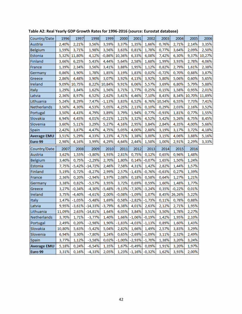
42

Table A2: Real Yearly GDP Growth Rates for 1996-2016 (source: Eurostat database)

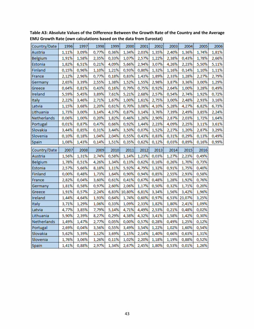
43

Table A3: Absolute Values of the Difference Between the Growth Rate of the Country and the Average

EMU Growth Rate (own calculations based on the data from Eurostat)

44

Figure A1: Scatter Plots of Independent Variables vs. Date

G is the change in the government spending, I is the change in the private investment, In is the inflation

rate and E is the number of employed people.

Table A4: Correlations Among Independent Variables

45

Figure A2: Scatter Plots of Residuals vs. Independent Variables