the great recession in the non-emu visegrád countries: a

Finance a úvěr-Czech Journal of Economics and Finance, 66, 2016, no. 3 207

JEL classification: E37, E44, E63 Keywords: DSGE model, Great Recession, time-varying parameters, particle filter, financial frictions

The Great Recession in the Non-EMU Visegrád

Countries: A Nonlinear DSGE Model

with Time-Varying Parameters*

Stanislav TVRZ—National Bank of Slovakia and Faculty of Economics and Administration, Masaryk University, Brno, corresponding author ([email protected])

Osvald VAŠÍČEK—Faculty of Economics and Administration, Masaryk University, Brno ([email protected])

Abstract

Inspired by the radically different course and aftermath of the Great Recession in the Polish

economy and the economies of the Czech Republic and Hungary in contrast to their

comparable economic development before the crisis, we investigate the structural sta-

bility of these three Central European economies in that period. The question of struc-

tural stability is essential for proper application of a standard DSGE model in a given

economy. In the case of significant structural changes, these should be incorporated

explicitly into the model structure in order to avoid misleading results. Each of the three

economies is represented by a nonlinear small open economy dynamic stochastic general

equilibrium model with a financial accelerator. First, the DSGE models are estimated

using Bayesian methods under the assumption of constant structural parameters. Then

the development of time-varying structural parameters is estimated by means of a particle

filter using second order approximation of a nonlinear DSGE model. We find several

statistically significant structural changes in the Czech and Polish economies. According

to the time-varying impulse response functions, the structural changes during the Great

Recession curbed the negative impacts of the adverse exogenous shocks to a certain

extent in the Czech and Polish economies. By contrast, the vulnerability of the Hungarian

economy further increased.

1. Introduction

The turbulent period of the Great Recession brought about distinct changes in the performance and behavior of the non-EMU Visegrád (NEV) economies of the Czech Republic, Poland and Hungary and highlighted their mutual differences. While the Polish economy avoided economic recession altogether, the Czech and Hungarian economies suffered a protracted and relatively deep double-dip recession. These differences might have been caused by the different size and composition of the exoge-nous shocks that these economies faced during this period, including the reaction of fiscal and monetary policy authorities. Alternatively, they could be related to the underlying structural differences. A different sectoral composition could be one

* The views expressed here are those of the authors and do not necessarily reflect the position of the NationalBank of Slovakia The authors would like to thank Daniel Němec, Jaromír Tonner and Jan Brůha for their advice and helpful comments. Access to computing and storage facilities owned by parties and projects contributing tothe National Grid Infrastructure MetaCentrum, provided under the programme “Projects of Large Research, Development, and Innovations Infrastructures” (CESNET LM2015042), is greatly appreciated.This contribution is the result of the Masaryk University research project MUNI/A/1040/2015.

208 Finance a úvěr-Czech Journal of Economics and Finance, 66, 2016, no. 3

example of such long-term structural differences. Since the NEV economies are converging economies and could even be considered emerging markets, they are continuously undergoing important structural changes and the pace of these struc-tural changes may be very different in the three economies. One example of such an ongoing structural change is increasing engagement in international trade and growing openness. Conceivably, other temporary structural changes might have occurred during the period of the Great Recession due to the extraordinary events experienced at that time. For example, commercial banks might have become more cautious or even reluctant to lend money in times of uncertainty.

The growing popularity of the dynamic stochastic models of general eco-nomic equilibrium (DSGE models) in recent decades has led to their common use in academia as well as in professional circles. The DSGE models are also employed in the central banks of the NEV economies as either the main or auxiliary tool in the regular macroeconomic prediction process. Usually, the standard DSGE models work with an assumption of stable structural model parameters. Therefore, the ques-tion of structural stability is essential for proper application of a DSGE model in a given economy. In the case of significant structural changes, these should be incorporated explicitly into the model structure in order to avoid misleading results.

The goal of this paper is to identify and compare the most important changes in the structure of the NEV economies during the turbulent period of the Great Recession and the subsequent recovery. We also want to find out what the implica-tions of the identified structural changes are for the behavior of the model economy. For that purpose, we estimate three DSGE models of a small open economy for the NEV countries. Time-varying structural parameters are assumed in all three models, rendering them nonlinear. Filtration of the models is performed with the use of a nonlinear particle filter (NPF) to identify the unobserved trajectories of the time-varying parameters.

The results presented in this paper are the outcome of a line of research whose earlier results were published in Tvrz and Vašíček (2014) and Tvrz (2015). In this paper, we elaborate on our previous research and present a comprehensive set of empirical results focused on the NEV economies. The question of structural stability of the US economy was studied by Fernández-Villaverde and Rubio-Ramírez (2007) using a medium-scale DSGE model and allowing for parameter drifting. The authors found a strong evidence of structural changes. Identified changes in the pricing behavior of firms and households captured by respective Calvo parameters were the most pronounced. Kulish and Pagan (2013) developed solutions for linearized DSGE models with structural changes about which eco-nomic agents have various kinds of beliefs. The subject of the structural stability of the small Central European economies was previously investigated by, for example, Vašíček et al. (2011), who found evidence of parameter drifting in the Czech data, and Čapek (2012), who compared a recursive estimation approach to non-linear filtration. Structural differences in the labor markets of the four Visegrád countries were investigated by Němec (2013). The implications of financial frictions for the monetary policy of the Czech small open economy were investigated in detail in Ryšánek et al. (2012). The effects of financial frictions in the Polish economy were studied by Brzoza-Brzezina and Kolasa (2013) and Brzoza-Brzezina et al. (2013).


Figure 1 Real GDP (index, 100 = pre-crisis maximum)

Source: Eurostat.

The repercussions of the shocks originating in the financial sector in the Hungarian economy were explored by Tamási and Világi (2011).

We find statistically significant changes in the values of several structural parameters in the Czech economy during the Great Recession and in the Polish economy during the earlier period of 1999–2003. In the case of the Hungarian economy, no statistically significant changes as distinguished by the 95% HPDI intervals were identified. However, several parameters show a similar degree of vola-tility in relative terms as in the case of the Czech economy. According to the time-varying impulse response functions, the structural changes during the Great Recession curbed the negative impacts of the adverse exogenous shocks to a certain extent in the Czech and Polish economies. By contrast, the vulnerability of the Hungarian economy further increased. In recent times, the time-varying parameter estimates in all three economies have been in the vicinity of their respective initial values and these economies seem to have stabilized.

The structure of this paper is as follows: Section 2 describes the common features and the main differences in economic development in the NEV countries during the Great Recession. Section 3 describes the main features of the small open economy DSGE model that is used for the analysis. Section 4 explains the basic principles of the estimation technique of the nonlinear particle filter. Section 5 describes the input data, the data sources and preliminary transformations. Section 6 contains the calibration. Section 7 presents the empirical results together with their economic interpretation. Section 8 concludes the paper with a summation of its main findings.

2. Developments in the NEV Countries

What is particularly interesting is the differing effects of the Great Recession on the real economic output of the Polish economy and the other two NEV economies. The Czech economy suffered a double-dip recession with a relatively deep economic downturn between 2008Q4 and 2009Q2 and a protracted shallow recession between 2011Q4 and 2013Q1. Developments in the Hungarian economy were similar. A deep recession between 2008Q3 and 2009Q3 was followed by a less severe recession in 2012. By contrast, the Polish economy experienced only a minor economic slow-down in 2008Q4 and avoided recession altogether. While Poland became an exem-plary case of successful crisis avoidance, the Czech and Hungarian economies stalled.


Figure 2 Interest Rates on New Mortgages (percent) and Lending Margins on Loans for Housing (percentage points)

Notes: interest rates—lines, left axis, lending margins—circles, right axis

Source: European Central Bank.

Between Poland’s accession to the European Union in 2004 and its pre-crisis economic peak, the Polish economy grew by an average quarterly rate of 1.27%, while the Czech economy grew by a similar quarterly average rate of 1.32%, and the Hungarian economy grew on average by 0.75% per quarter. Since 2010, the Polish economy has been growing by an average quarterly rate of approximately 0.75%. In the same period, the Czech economy has achieved an average quarterly rate of real GDP growth of only 0.25%, while the Hungarian economy has grown by an average quarterly rate of 0.33%. As can be seen in Figure 1, the Polish economy was approaching 120% of its pre-recession peak in 2014Q4, while the Czech real output was finally returning to its maximum of six years before and Hungarian GDP was almost back to its pre-crisis volume by early 2015.

The banking sector of the non-EMU Visegrád countries coped with the finan-cial crisis of 2007–2008 fairly well, mainly thanks to the fact that their domestic banks were not trading with complex structured financial instruments in significant volumes and their exposure to the US subprime mortgage crisis was therefore limited.1 However, the NEV economies were affected by the increase of systemic risk and uncertainty during the second half of 2008, which led to a downturn in world aggregate demand and international trade. Even though the NEV economies were relatively sheltered from the first-hand effects of the global financial crisis, they were hit by the subsequent global economic crisis like the rest of the globalized world economy.

Figure 2 shows interest rates on new mortgages and lending margins2 on loans for house purchases in the NEV economies. An increase in interest rates in 2007– –2008 can be distinguished in all three economies. Since the lending margins in the Czech economy stayed unchanged, this development reflects the tightening of monetary policy in that period. Mortgage interest rates were kept unchanged

1 In the Czech economy, the spread between the PRIBOR interbank offered rate and the interest rate on loans to non-financial corporations increased by approximately one percentage point during the crisis. 2 According to the European Central Bank (2000), the lending margin is defined as “the difference between

banks’ average contractual rates on new loans (flows) and a reference rate. The reference rate is the market

interest rate of a corresponding average maturity representing the financial opportunity cost for banks. It is not intended to represent the (marginal) cost of funds for the bank.”


Figure 3 Nominal Exchange Rates (index, 100 = 2008M07)

Source: European Central Bank.

in the Czech economy through 2009, while the policy interest rate and the oppor-tunity cost of the commercial banks declined. This decoupling of the commercial and policy interest rates is reflected in increased lending margins and is a manifestation of financial frictions in the Czech economy. Similar development can be observed in the Polish economy. However, the lending margins in Poland began to increase during 2008, which suggests that the Polish commercial banks perceived the increased riskiness on the mortgage market earlier than those in the Czech Republic. The situa-tion in Hungary is very specific. While mortgage interest rates increased by 3.5 pp between January 2008 and February 2009, the lending margins declined from around 4% to below zero in 2008Q4. This extraordinary development was mainly caused by the fact that the Hungarian central bank increased its policy rate in October 2008, from 8.5% to 11.5%, in order to defend the forint and mitigate depreciation pressures during the crisis. As the policy interest rate did not return below 8.5% before August 2009, the opportunity costs of Hungarian banks actually increased during the crisis and, as a result, their lending margins plunged. While the effects of financial frictions during the Great Recession can be distinguished quite clearly in the Czech and Polish economies, the situation in Hungary is blurred by the currency crisis.

In the Czech and Polish economies, currency depreciation helped exporters to maintain their competitiveness during the crisis. The Czech currency depreciated by approximately 20%, while the Polish currency depreciated by more than 40%. In Figure 3, we can see that the pre-crisis development of the Czech and Polish currencies in relation to the euro was very similar and a significant gap opened as late as during the crisis. Even after the exchange rate intervention of the Czech National Bank (CNB) in November 2013, which led to a devaluation of the Czech currency in relation to the euro by approximately 5%, the Polish currency was still by approxi-mately 12 percentage points weaker in comparison with its pre-crisis peak than the Czech currency.

The much more substantial depreciation of the Polish currency can be attributed in part to the more vigorous loosening of monetary policy in the Polish economy. The three-month interest rate declined by nearly ten percentage points during 2009 and 2010 in Poland and reached 6%, while in the Czech Republic it declined by approximately 4.5 percentage points and reached 1.2%. Thus, the Polish


Figure 4 General Government Debt and Deficit (percent of GDP)

Notes: debt—left axis, deficit—right axis. Source: Eurostat.

economy probably benefited from a much larger space for the loosening of monetary policy.

However, the situation in Hungary and, to a certain extent, Poland was com-plicated by the large share of debt denominated in foreign currencies (especially Swiss francs), which had been accumulated in the favorable period when the domes-tic currency was strong and low foreign interest rates seemed appealing. In July 2008, the share of household debt denominated in a foreign currency was almost 60% in Hungary, while in Poland it was less than 30% and in the Czech Republic the share was negligible. The rapid currency depreciation in 2008Q4 (see Figure 3) amplified the burden of debt denominated in foreign currencies and led to a currency crisis, which exacerbated the impact of the Great Recession. Between July 2008 and January 2009, the share of loans to households denominated in a foreign currency increased to almost 70% in Hungary, while in Poland it reached approximately 40%. The appreciation of the Swiss franc in 2011 further complicated the situation and eventually resulted in a government-led initiative to convert foreign currency mort-gages into domestic currency mortgages. The share of foreign currency household debt in Poland fell back below 30% during 2014; nevertheless, appreciation of the Swiss franc had a relatively serious impact and provoked a discussion about ways of sharing the incurred losses between debtors and banks.

Among other factors, the divergent development of the NEV economies since the Great Recession was reinforced by differences in fiscal policy. As can be dis-cerned in Figure 4, Polish economic growth was reignited by increased government spending after the impact of the crisis. The deficits of the crisis years 2009 and 2010 reached values near 7.5%. However, since comparatively high economic growth was restored, the debt-to-GDP ratio increased by only 11.5 pp between 2007 and 2013. In Hungary, the currency crisis and subsequent IMF intervention resulted in rela-tively restrained fiscal policy during the crisis, with deficits around 5%. The debt-to-GDP ratio increased by only 11.4 pp between 2007 and 2013 thanks to high inflation (see Figure 5). In the Czech economy, tight fiscal policy was maintained during the crisis. With deficits similar to those in Hungary, the debt to GDP ratio increased by nearly 18 pp between 2007 and 2013 due to a lack of economic growth and low inflation.

Since 2013, the NEV economies have faced strong disinflationary pressures (see Figure 5). While in Poland and Hungary the policy interest rates were still


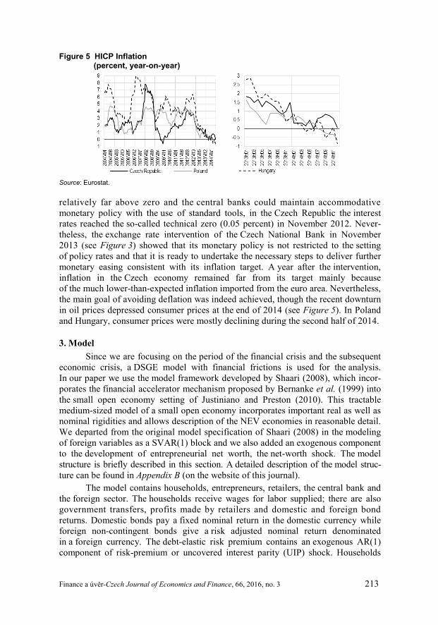
Figure 5 HICP Inflation (percent, year-on-year)

Source: Eurostat.

relatively far above zero and the central banks could maintain accommodative monetary policy with the use of standard tools, in the Czech Republic the interest rates reached the so-called technical zero (0.05 percent) in November 2012. Never-theless, the exchange rate intervention of the Czech National Bank in November 2013 (see Figure 3) showed that its monetary policy is not restricted to the setting of policy rates and that it is ready to undertake the necessary steps to deliver further monetary easing consistent with its inflation target. A year after the intervention, inflation in the Czech economy remained far from its target mainly because of the much lower-than-expected inflation imported from the euro area. Nevertheless, the main goal of avoiding deflation was indeed achieved, though the recent downturn in oil prices depressed consumer prices at the end of 2014 (see Figure 5). In Poland and Hungary, consumer prices were mostly declining during the second half of 2014.

3. Model

Since we are focusing on the period of the financial crisis and the subsequent economic crisis, a DSGE model with financial frictions is used for the analysis. In our paper we use the model framework developed by Shaari (2008), which incor-porates the financial accelerator mechanism proposed by Bernanke et al. (1999) into the small open economy setting of Justiniano and Preston (2010). This tractable medium-sized model of a small open economy incorporates important real as well as nominal rigidities and allows description of the NEV economies in reasonable detail. We departed from the original model specification of Shaari (2008) in the modeling of foreign variables as a SVAR(1) block and we also added an exogenous component to the development of entrepreneurial net worth, the net-worth shock. The model structure is briefly described in this section. A detailed description of the model struc-ture can be found in Appendix B (on the website of this journal).

The model contains households, entrepreneurs, retailers, the central bank and the foreign sector. The households receive wages for labor supplied; there are also government transfers, profits made by retailers and domestic and foreign bond returns. Domestic bonds pay a fixed nominal return in the domestic currency while foreign non-contingent bonds give a risk adjusted nominal return denominated in a foreign currency. The debt-elastic risk premium contains an exogenous AR(1) component of risk-premium or uncovered interest parity (UIP) shock. Households


then spend their earnings on consumption and on acquisition of domestic and foreign bonds.

3.1 Entrepreneurs

Entrepreneurs play two important roles in the model. They run wholesale goods-producing firms and they produce and own capital. The intermediate goods market and the capital goods market are assumed to be competitive. Wholesale goods production is affected by domestic productivity AR(1) shocks and capital goods pro-duction is subject to capital adjustment costs. Entrepreneurs finance the production and ownership of capital Kt from their net worth Nt and borrowed funds. The cost of borrowed funds is influenced by the borrower’s leverage ratio via the external finance premium

1

tt

t t

NEFP

Q K

χ−

−

=

(1)

where Qt is the real price of capital or Tobin’s Q and χ is the financial accelerator parameter. To maximize profit, entrepreneurs choose the optimal levels of capital and borrowed funds.

In each period a proportion ( )1 NWtA ς− of entrepreneurs leaves the market and

their equity ( )1 NWt tA Vς− is transferred to households in the form of transfers. NW

tA

is a shock in entrepreneurial net worth. It influences the development of net worth by changing the bankruptcy rate of entrepreneurs, as its positive innovations increase the survival rate of entrepreneurs. Its logarithmic deviation from a steady state is assumed to evolve according to an AR(1) process. ς is the steady-state bankruptcy

rate.

3.2 Retailers

There are two types of retailers in the model—domestic goods retailers and foreign goods retailers. Both are assumed to operate in conditions of monopolistic competition. Domestic goods retailers buy domestic intermediate goods at the whole-sale price and sell the domestic final goods to consumers. Foreign goods retailers buy goods from foreign producers at the wholesale price and resell the foreign goods to domestic consumers. The difference between the foreign wholesale price expressed in the domestic currency and the foreign final goods price, which is a deviation from the law of one price (LOP), is determined by the exogenous AR(1) shock. Nominal rigidities are introduced into the model by means of Calvo-type price setting and the inflation indexation of retailers.

3.3 Central Bank

The central bank determines the nominal interest rate in accordance with the following forward-looking Taylor interest rate rule (small-letter variables denote deviations from the steady state, which implies a gap):

( ) ( ) ( )1 1 11 MP

t t t y t ti i E E yπρ ρ β π Θ ε− + + = ⋅ + − ⋅ ⋅ + ⋅ + (2)


where ti is the nominal policy interest rate, ρ is a smoothing parameter, πβ is

the weight parameter of expected inflation ( )1tE π + and yΘ is the weight parameter

of the expected output gap ( )1tE y + . Deviations of the interest rate from the interest

rate rule are explained as monetary policy i.i.d. shocks MPtε .

3.4 Foreign Sector

Following Christiano et al. (2011), the foreign economy variables—real out-put, consumer price index (CPI) inflation and the nominal interest rate—are modeled using a structural SVAR(1) model as described in equation (3).

*

* * * * * *

*

* * * * * * * *

*

* * * * * * * * * *

* *1

* *1

* *1

1 0 0

1 0

1

ytt ty y y y i

t t ty i y

it t ti y i i i i y i

y y

i i

ππ

π π π π π

π π

ερ ρ ρ

π ρ ρ ρ π σ ε

ρ ρ ρ σ σ ε

−

−

−

= +

(3)

3.5 Time-Varying Parameters

All the estimated model parameters are considered time-varying with the excep-tion of shock autoregression parameters and standard deviations. Time-varying para-meters are defined as unobserved endogenous variables with the following law of motion:

( ) 11t t t t t

θ θ θθ α θ α θ ν−= − ⋅ + ⋅ + (4)

where tθ is a general time-varying parameter, θ is the initial value of this para-

meter, tθα is a time-varying adhesion parameter common for all the remaining time-

varying parameters and ( ) 0,~t Nθ θνν σ is an exogenous innovation in the value

of parameter tθ . The setting of the adhesion parameter tθα influences the tendency

of the time-varying parameter tθ to return to its initial value θ . With 0tθα = ,

the time-varying parameter would be defined as random walk, while with 1tθα = ,

the parameter would be white noise centered around the initial valueθ .

For the purposes of this paper, tθα is itself considered to be time-varying. Its

adhesion parameter αα is set to the fixed value of 0.01, its initial value is set to

the value of 0.25θα = and its exogenous innovations tαν follow (0, 0.5)N distri-

bution:

( ) 11t t t

θ α θ α θ αα α α α α ν−= − ⋅ + ⋅ + (5)

The adhesion parameter is therefore virtually free to drift away from its initial

value. The choice of the calibration of the initial value of the adhesion parameter 0θα

does not qualitatively change the results. Sensitivity analysis was performed with

the value of θα set to 0.01, 0.05, 0.10, 0.25 and 0.50. The persistence of the iden-


Figure 6 Nonlinear Particle Filter

Source: Authors.

tified trajectories of the time-varying parameters is greater for the lower values of adhesion. However, the main characteristics of the development identified (such as the direction and timing of major shifts in the value of a given parameter) stay more or less the same.

4. Estimation Technique

A nonlinear particle filter (NPF) is used in this paper to identify the unob-served states of the DSGE model. Under the assumption of time-varying structural parameters, the log-linear model equations become nonlinear in their parameters. In this section we briefly describe the main principles of this nonlinear particle filter.

4.1 Nonlinear Particle Filter

Unlike the basic Kalman filter, which is optimal only for linear systems with Gaussian noise, the nonlinear particle filter is a more sophisticated tool that can be used even for nonlinear state-space systems with non-Gaussian noise. In this section, we provide only the basic principles of the algorithm. A detailed description can be found in, for example, Haug (2005).

Figure 6 contains a diagram of the NPF algorithm. In condensed form, the NPF algorithm can be described as follows:

1. Initialization: 0,=t set the prior mean 0x (steady state) and covariance matrix

0P for the state vector tx .

2. Generating particles: Draw a total of N particles ( ) , 1, ,= …it i Nx from distribu-

tion ( )tp x with mean tx and covariance matrix tP .

3. Time Update: 1= +t t , for each particle ( 1, , )= …i N propagate the particle into the future with the use of a nonlinear transition and measurement equation and calculate means ( )| 1t t−x , ( )| 1t t−y and covariance matrices ( )| 1 −t t

P , ( )|y yP , ( )|x y

P .

4. Kalman filter: Calculate Kalman gain ( ) 1

( | ) ( | )

−=t x y y yK P P , ( ) ( )( )| 1 | 1t t tt t t t− −= + −x x K y y

and ( ) ( )( | )| 1−= −T

t t y y tt tP P K P K .

5. If , < maxt t continue with step 2; otherwise end the computation.

In our application we performed 20 runs of the NPF with 30,000 particles each3 for a second order approximation of the nonlinear DSGE model.

3 The setting of the particle simulation is chosen as a compromise between accuracy and the time demands of the calculation. By experimenting with the setting of the particle filter algorithm, we found that the results do not change significantly when the number of runs or the number of particles is increased.

Generating Particles

Initialization

Time Update

Kalman Filter


4.2 Initial Values

Before the application of the NPF algorithm, we estimated the model with constant parameters to obtain estimates of the autoregression parameters and standard deviations of structural shocks that are considered constant even in the NPF. Also, the posterior means of the structural parameters were used as initial values of the time-

varying parameters ( )θ in the NPF estimation. Standard deviations of time-varying

parameter innovations ( )θνσ were set proportionally to the posterior means4 of the model

with constant parameters (10%). Constant model parameters were estimated using a Random Walk Metropolis-Hastings algorithm as implemented in the Dynare tool-box for Matlab (see Adjemian et al., 2011). Two parallel chains of 500,000 draws each were generated during the estimation. The first 50% of draws were discarded as a burn-in sample. The scale parameter was set to achieve an acceptance rate of around 30%.

5. Data

Quarterly time series of eight observables were used for the purposes of esti-mation. These ESA 2010 consistent time series cover the period between the first quarter of 1999 and the third quarter of 2014 and contain 63 observations. Graphs of the observed time series are included in Appendix C (on the website of this journal).

Seasonally adjusted time series of real gross domestic product (GDP), the har-monized consumer price index (CPI), the three-month policy interest rate (interbank offered rate) and real investment are used for the domestic economy. The foreign sector is represented by the 17 euro-area countries and its development is captured by the seasonally adjusted time series of real GDP, CPI and the three-month policy interest rate. Time series of the CZK/EUR, PLN/EUR and HUF/EUR real exchange rates are also used for the purposes of estimation. These time series were obtained from the databases of Eurostat, the Czech National Bank, Polish National Bank, Hungarian National Bank and European Central Bank.

The original time series were transformed prior to estimation so as to express logarithmic deviations from their respective steady states. The logarithmic deviations of the observables from their trends were calculated with the use of a Hodrick-Prescott (HP) filter.5 In order to mitigate the end-of-sample bias of the HP-filter, the level data were extended with a VAR forecast6 before calculation of the loga-rithmic deviations.

4 This choice was motivated by the big differences in posterior standard deviations of estimated constant parameters (relative to the posterior means). Posterior standard deviations would be the natural alternative; however, they capture uncertainty associated with the posterior estimate that need not have any relation to the stability of the posterior estimate in time. The parameter in question could be time-invariant and yet hard to estimate, which would yield high posterior standard deviation. Therefore, we decided to calibrate the standard deviations of the time-varying parameters in a uniform way and let the filtration decide which parameters are time-varying. 5 The parameter of the HP filter λ was set to 1600, a value commonly used for quarterly data. 6 A VAR(3) model was considered for the foreign economy, while a VAR(1) model with three exogenous foreign variables was considered for the domestic economy. A forecast for the next eight quarters was calculated.


6. Calibration

We decided to calibrate several deep structural parameters because they are difficult to estimate. These parameters were assigned values commonly reported in the literature. The value of discount factor β of 0.995 implies a real interest rate of approximately 2% per annum. The capital share in production α corresponds to a national income share of capital of 0.35. Values of around one-third are commonly used in the literature. A capital depreciation rate δ of 2.5 percent per quarter is also quite standard. Households’ share of the labor supply Ω is calibrated according to Shaari (2008) to 99%, which leaves the remaining 1% of the labor supply to be provided by entrepreneurs. The calibration of steady-state markup μ to 1.2 is in line with Shaari (2008).

7. Empirical Results

In this section, we first look at the structural differences between the NEV economies as captured by the constant posterior estimates of the model parameters. We then make a few remarks about the development of selected unobserved endogenous variables and, finally, we turn to the comparison of the time-varying parameter estimates and their interpretation in terms of representative economic agents’ behavior.

7.1 Posterior Estimates

Prior densities of the estimated structural parameters are presented in Table 1. The prior densities are the same for all three economies in order to identify the struc-tural differences in the data.

A comparison of the posterior estimates of all three economies is presented in Table 2. Priors and posteriors of the remaining model parameters are included in Appendix A. Graphs of prior and posterior densities as well as Brooks and Gelman (1998) convergence diagnostics are included in the technical Appendix C.

While the multivariate convergence diagnostics do not indicate any problems, the graphs of prior and posterior densities show a lack of information about the para-meter of consumption habit Y in the data. The bimodal posterior densities of several parameters in the Hungarian model hint at possible structural changes. Most of the parameters are estimated to be very similar in all three economies, but there are also some interesting differences.

The difference in preference bias to foreign goods γ can be explained by the greater openness of the export-oriented Czech and Hungarian economies in comparison to the relatively self-sustaining Polish economy. In terms of the exports-to-GDP ratio, the Hungarian economy is actually more open than the economy of the Czech Republic. However, given the large share of foodstuffs in the consump-tion basket of households, the estimate may be influenced by the relatively self-sufficient agricultural sector in Hungary and relatively larger share of imported groceries in the Czech economy.

The lower debt-elastic risk premium elasticity Bψ in the Czech economy sug-

gests that forex dealers are less sensitive about the external balance of the Czech economy in relation to the exchange rate, which correlates to its status as a regional


Table 1 Prior Densities (Structural Parameters)

Parameter Distribution Prior

Mean Std

Structural parameters

Υ Habit persistence B 0.60 0.05

Ψ Inv. elast. of lab. supply G 2.00 0.50

ΨB Debt-elastic risk premium G 0.05 0.02

η Home/foreign elast. subst. G 0.65 0.10

κ Price indexation B 0.50 0.10

γ Pref. bias to foreign goods B 0.40 0.15

ΘH Home goods Calvo B 0.70 0.10

ΘF Foreign goods Calvo B 0.70 0.10

Ψl Capital adjustment costs G 20.0 5.00

Financial frictions

Γ Capital/net worth ss ratio G 1.50 0.05

ζ Bankruptcy rate B 0.025 0.005

χ Financial accelerator G 0.05 0.01

Taylor rule

ρ Interest rate smoothing B 0.50 0.20

βπ Inflation weight G 1.50 0.20

Θy Output gap weight G 0.50 0.20

Notes: B—beta distribution, G—gamma distribution

Source: Authors’ calculations.

safe haven for investors. This probably results from the transparent monetary policy of the CNB and relatively tight fiscal policy.

The lower price indexation to past inflation κ in the Czech economy than in the other NEV economies is probably caused by the higher and more volatile inflation in Poland and Hungary. The Calvo parameters are estimated to be nearly the same for the Czech Republic and Poland; however, in Hungary the estimates are somewhat lower, suggesting greater flexibility of prices. Higher capital adjustment costs Iψ in Hungary and Poland suggest lower investment efficiency.

The parameters of financial frictions are estimated to be nearly the same in all three economies. This may be explained by the fact that most commercial banks operating in these economies are subsidiaries of large international groups, which treat the Central and Eastern European markets in a similar way.

The estimated parameters of the Taylor rule correspond to the fact that the cen-tral banks in the NEV countries operate independently in more or less strict inflation targeting regimes.

As can be seen in Table 2, the relaxation of the assumption of constant struc-tural parameters led to an improvement of log marginal likelihood of the DSGE models in all the NEV economies. The improvement was comparable in the case of the Czech and Polish economies, while it was less substantial in the Hungarian economy.


Table 2 Comparison of Posterior Means (Structural Parameters)

Parameter CZ PL HU


Υ Habit persistence 0.59 [1] 0.59 [0.99] 0.59 [0.99]

(0.053) [1] (0.053) [1.00] (0.054) [1.01]

Ψ Inv. elast. of lab. supply 1.26 [1] 1.31 [1.04] 1.36 [1.08]

(0.31) [1] (0.32) [1.04] (0.33) [1.09]

ΨB Debt-elastic risk premium 0.02 [1] 0.04 [1.78] 0.05 [2.09]

(0.007) [1] (0.013) [1.92] (0.017) [2.52]

η Home/foreign elast. subst. 0.61 [1] 0.59 [0.96] 0.60 [0.98]

(0.086) [1] (0.048) [0.56] (0.052) [0.61]

κ Price indexation 0.28 [1] 0.35 [1.24] 0.38 [1.36]

(0.074) [1] (0.084) [1.14] (0.1) [1.35]

γ Pref. bias to foreign goods 0.29 [1] 0.21 [0.74] 0.23 [0.82]

(0.067) [1] (0.041) [0.61] (0.056) [0.84]

ΘH Home goods Calvo 0.81 [1] 0.77 [0.96] 0.70 [0.86]

(0.024) [1] (0.029) [1.20] (0.059) [2.49]

ΘF Foreign goods Calvo 0.79 [1] 0.80 [1.01] 0.66 [0.84]

(0.031) [1] (0.027) [0.88] (0.066) [2.17]

Ψl Capital adjustment costs 28.71 [1] 33.32 [1.16] 36.18 [1.26]

(4.86) [1] (5.45) [1.12] (5.77) [1.19]

Financial frictions

Γ Capital/net worth ss ratio 1.47 [1] 1.47 [1.00] 1.47 [1.00]

(0.047) [1] (0.047) [1.01] (0.047) [1.00]

ζ Bankruptcy rate 0.031 [1] 0.029 [0.93] 0.029 [0.91]

(0.006) [1] (0.005) [0.95] (0.005) [0.93]

χ Financial accelerator 0.038 [1] 0.042 [1.12] 0.040 [1.05]

(0.007) [1] (0.008) [1.12] (0.008) [1.12]

Taylor rule

ρ Interest rate smoothing 0.86 [1] 0.66 [0.76] 0.68 [0.79]

(0.022) [1] (0.04) [1.86] (0.067) [3.11]

βπ Inflation weight 1.92 [1] 1.99 [1.03] 2.00 [1.04]

(0.22) [1] (0.22) [1.00] (0.24) [1.07]

Θy Output gap weight 0.11 [1] 0.21 [1.86] 0.22 [2.01]

(0.04) [1] (0.07) [1.89] (0.08) [2.08]

Log-marginal likelihood difference (time-varying—constant parameters)

18.95 22.85 5.93

Notes: Standard deviations in parentheses, relative to the Czech Republic in brackets.


7.2 Filtered Shock Innovations

Graphs of filtered shock innovations are included in Appendix C. These filtered innovations show the turbulent period of the Great Recession as being similar in all three NEV economies. A strong negative shock came from the external environ-ment via negative innovations in foreign output and, as a result, foreign demand for domestic exports dropped in the last quarter of 2008 and the first quarter of 2009.


There were also noticeable disinflationary pressures from abroad in the last quarter of 2008. Within the NEV economies, a substantial positive innovation closed the law- of-one price gap as importers lowered their profit margins during the crisis. Negative innovations in entrepreneurial net worth increased the number of bankruptcies during 2008–2009, which exacerbated the recession. There were also negative innovations in domestic productivity in the first half of 2009. The large depreciations of the NEV currencies are explained in part by large negative innovations in the UIP shock at the turn of 2008 and 2009. The biggest negative UIP shock came in the Polish economy, which helps to explain the large currency depreciation there. The deprecia-tion of the Hungarian currency was limited by a relatively restrictive monetary policy, indicated by large positive monetary policy shocks during the crisis.

The economic slowdown of 2012 is explained by a downturn of productivity, foreign demand and entrepreneurial net worth. The positive innovations of the LOP shock indicate a decline in importers’ profit margins. Large negative innovations in the UIP shock explain the depreciation of the Polish zloty and Hungarian forint. According to the monetary policy shock innovations, the relatively loose monetary policy in 2011 was tightened during 2012 in these two countries in particular. The exchange rate intervention of the CNB is captured as a negative innovation of the UIP shock at the turn of 2013 and 2014. More recently, we can see a series of negative innovations of the foreign price shock that translate to disinflationary pressures through import prices. On the other hand, a sequence of positive net-worth shock innovations indicates an improvement in the availability of financing and explains the pickup in investment.

It is also worth noting the large shocks in the entrepreneurial net worth in Poland and Hungary before their accession to the European Union in 2004. A series of negative net-worth shock innovations in Poland in 2001 corresponds to a period of economic difficulties7 in the aftermath of the 1998 Russian crisis. After a period of loose monetary policy, monetary policy was eventually tightened in order to reduce the macroeconomic imbalances incurred, which led to a plunge in invest-ment in 2001. While the Polish crisis had many internal and external causes, the model explains it in part with a net-worth shock. Large innovations of the net-worth shock in Hungary in 2003 can be directly related to the turbulent period of large-scale capital outflow. During that period, large macroeconomic imbalances caused by the expansionary fiscal policy in previous periods became evident and an open conflict about the policy mix erupted between the government and the cen-tral bank. A period of exchange rate turbulence, major policy interest rate hikes and capital outflow ensued.

7.3 Filtered Time-Varying Parameters

Figure 7 contains the filtered trajectories of selected time-varying parameters in the Czech and Polish economies. Only the parameters with more pronounced deviations from their initial values were selected (deviations larger than ±1percent).

7 Between 1998 and 2002 the unemployment rate in Poland doubled and reached 20%. The Polish central bank lowered interest rates in 1998 and 1999 by 11 pp to 13% due to the prospect of falling inflation. As inflation increased and reached 10% in 2000, the central bank gradually increased interest rates by a total of 6 pp to 19%.


Figure 7 Comparison of Selected Time-Varying Parameters (CZ vs.PL)

Notes: Percentage deviations from initial values, CZ—black solid line, PL—grey solid line.


To assess the statistical significance of the changes in the values of the time-varying parameters, we considered the 95% HPDI intervals obtained in the estimation with constant parameters. In the case of the Czech economy, the domestic goods Calvo parameter ( )Hθ and the leverage ratio parameter ( )Γ deviated outside of their HPDI

intervals in the 2006–2009 period. In the case of the Polish economy, the domestic and foreign goods Calvo parameters ( ),H Fθ θ , elasticity of substitution between foreign

and domestic goods parameter ( )η and the leverage ratio parameter ( )Γ exceeded

the bounds of their particular HPDI intervals in the 1999–2003 period.

Apart from the period of 1999–2003, when the Polish economy slowly recovered from the aftermath of the 1998 Russian crisis, the filtered trajectories of the Polish economy show much lower volatility in comparison to the Czech econ-omy. This result can be partially explained by the greater diversification of the Polish economy, which is 2.5 times as large as the Czech economy, and also by its lower openness to international trade8, which makes it more resilient to foreign crises.

In the following part of this section, we attempt to interpret the identified changes in the values of structural parameters in the Czech and Polish economies in terms of economic agents’ behavior.

8 The share of nominal exports in GDP was 0.75 in the Czech Republic and 0.44 in Poland in 2013.


The development of the financial accelerator parameter χ (the elasticity of the external finance premium with respect to the leverage ratio) in the Czech economy suggests that the reaction of the commercial banks to the deteriorating leverage ratio in 2008 was subdued. Commercial interest rates were probably not raised sharply due to initial optimism about the length and extent of the financial crisis. However, after the first quarter of 2009, the impact of the financial crisis on the real economy was becoming evident and the sensitivity of the external finance premium began to rise again. In the case of Poland, the decline of sensitivity was not as substantial.

The trajectory of the steady-state leverage ratio Γ in the Czech economy captures the improving conditions in the economic boom period of 2007–2008, when firms were becoming less dependent on external funding. The situation, however, worsened quickly during the 2008–2009 crisis. In Poland, the development of this parameter was qualitatively similar, but the magnitude of the deviations from the initial value was much smaller. However, large deviations of this parameter can be distinguished in 2002 and 2003. The low leverage ratio in this period was prob-ably one of the consequences of the Russian crisis, and its subsequent increase should be perceived as a positive development enabled by decreased uncertainty in the Polish economy.

Capital adjustment costs Iψ exhibit an increase during 2008 and 2009 in the Czech

and Polish economies, suggesting that clear investment opportunities were becoming scarce and investment efficiency was declining. Again such deviations are much larger in the Czech economy.

The trajectories of elasticity between domestic and foreign goods η and foreign goods’ share in consumption γ have the potential to partially explain the dif-ferences between the effects of the Great Recession in the two economies. Both these parameters increased significantly in the pre-crisis period in the Czech economy, thus boosting the volume of international trade together with the dependency of the Czech economy on the external environment. The negative effects of this development materialized in late 2008 and early 2009. By comparison, the development of import share γ in the Polish economy was much steadier during the Great Recession. How-ever, our results suggest that the Polish economy underwent structural changes of a similar order of magnitude during the 2000–2003 crisis. After a successful restructuring of the industrial sector of the economy and reorienting on new export markets, the Polish economy lowered its dependence on the external environment.

The substantial decline of the debt-elastic risk premium ΨB in the Czech

economy during the 2008–2009 crisis suggests that the Czech koruna was still perceived to be a regional safe haven, but the government’s announced austerity measures probably played an important role as well. Therefore, the Czech currency did not depreciate as much as the other NEV currencies despite the negative eco-nomic outlook. In Poland, the decline of the debt-elastic risk premium was only marginal.

The filtered trajectories of the Calvo parameters show declining rigidity in the prices of domestic goods Hθ during 2007 and 2008. Demand and wage

growth were strong in this economic boom period. On the other hand, the rigidity


of the prices of imported goods Fθ is estimated to have increased, probably due to

the appreciation of the real exchange rate, which eased supply-side pressures. During 2009 the situation reversed as foreign demand faltered, domestic supply-side pressures eased and the real exchange rate depreciated. After 2010, the Calvo parameters returned to the vicinity of their respective initial values. In the Czech economy, the domestic Calvo parameter increased due to weak demand during the 2012–2013 recession, which intensified disinflationary pressures. After the Czech National Bank’s exchange rate intervention in the last quarter of 2013 put the prices of importers under pressure, the Calvo parameter of importing firms increased above its initial value. Since domestic demand in the Czech economy was relatively weak, importers were willing to absorb part of the cost increase, thus increasing price stickiness. The rising prices of imported goods (though limited) made room for domestic pro-ducers of substitute goods to slightly increase their prices as well, which is reflected in the decline of the domestic Calvo parameter. This development is in line with the expected impact of the exchange rate intervention as communicated by the Czech National Bank and would suggest that the intervention was successful in its main goal of preventing deflation in the Czech economy.

A comparison of the development of selected time-varying parameters in the Czech and Hungarian economies is depicted in Figure 8. In the case of the Hun-garian economy, no statistically significant changes as distinguished by the 95% HPDI intervals were identified. Nevertheless, several parameters such as the Calvo parameters ( ),H Fθ θ and the leverage ratio parameter ( Γ ) show a similar degree

of volatility in relative terms as in the case of the Czech economy. The development of financial accelerator χ is influenced by the aforemen-

tioned Hungarian currency crisis in 2003. During the Great Recession, this parameter remained stable and began to decline only recently. Similarly, the steady-state leverage ratio Γ declined during the 2003 crisis in Hungary. Unlike in the Czech and Polish economies, the leverage ratio increased during the Great Recession, probably due to currency depreciation and the large share of foreign currency debt. This develop-ment amplified the increase of the interest rate spread and further worsened the avail-ability of debt financing in Hungary. The capital adjustment costs parameter ΨI increased substantially during the 2003 crisis but remained mostly stable during the Great Recession.

The elasticity between domestic and foreign goods η and foreign goods’ share in consumption γ in Hungary increased during the 2006–2008 period, but the magni-tude of the deviations from initial values was subdued in comparison to the Czech economy, probably because of the fiscal consolidation in 2007. These two parameters returned to their initial values during 2010.

The debt-elastic risk premium ΨB declined in the Hungarian economy in 2008 and 2009 due to fiscal consolidation and austerity measures, but the decline was not as considerable as in the Czech economy.

The filtered trajectories of the Calvo parameters show a rapid increase in the ri-gidity of prices of domestic goods Hθ during 2009. Domestic as well as foreign

demand faltered and domestic supply-side pressures eased. Domestic retailers had to lower their profit margins and put price growth on hold. The rigidity of the prices


Figure 8 Comparison of Selected Time-Varying Parameters (CZ vs.HU)

Notes: Percentage deviations from initial values, CZ—black solid line, HU—black dashed line.


of imported goods θF is estimated to have decreased during the crisis. Currency depreciation together with falling demand led to a complicated situation for im-porters, who had to react swiftly to the price adjustments of competitors. During 2010, the Calvo parameters returned to the vicinity of their respective initial values.

The downward deviation of the inflation weight in the Taylor rule βπ in 2009 suggests that the monetary policy reaction should have been more radical in all three NEV economies. Interest rates probably should have been lowered faster in order to counter the growing external finance premium.

Figure 9 contains filtered trajectories of the time-varying adhesion parameter α

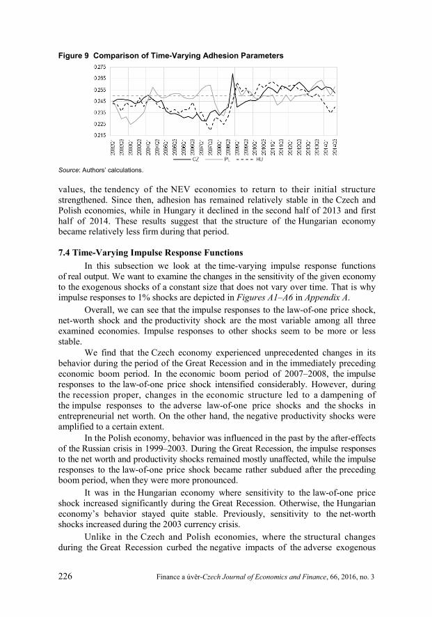
θ for all three NEV economies. The parameter reflects the general tendency of the re-maining time-varying parameters in a given economy to return to their initial values. The filtered values fluctuate around the initial value of 0.25, between a minimum of 0.22 and maximum of 0.27. We can distinguish a period of lower adhesion in the Czech and Hungarian economies in the economic boom period between 2005 and 2008. In the Polish economy, lower adhesion can be found in the period from 2002 to 2003, and then in 2008. The periods of lower adhesion often correspond to times when the economies underwent important structural changes. In general, the structural parameters deviated further away from their initial values in these periods. During the period of the main impact of the crisis in late 2008 and early 2009, we find slightly elevated adhesion. As many structural parameters reached exceptional


Figure 9 Comparison of Time-Varying Adhesion Parameters


values, the tendency of the NEV economies to return to their initial structure strengthened. Since then, adhesion has remained relatively stable in the Czech and Polish economies, while in Hungary it declined in the second half of 2013 and first half of 2014. These results suggest that the structure of the Hungarian economy became relatively less firm during that period.

7.4 Time-Varying Impulse Response Functions

In this subsection we look at the time-varying impulse response functions of real output. We want to examine the changes in the sensitivity of the given economy to the exogenous shocks of a constant size that does not vary over time. That is why impulse responses to 1% shocks are depicted in Figures A1–A6 in Appendix A.

Overall, we can see that the impulse responses to the law-of-one price shock, net-worth shock and the productivity shock are the most variable among all three examined economies. Impulse responses to other shocks seem to be more or less stable.

We find that the Czech economy experienced unprecedented changes in its behavior during the period of the Great Recession and in the immediately preceding economic boom period. In the economic boom period of 2007–2008, the impulse responses to the law-of-one price shock intensified considerably. However, during the recession proper, changes in the economic structure led to a dampening of the impulse responses to the adverse law-of-one price shocks and the shocks in entrepreneurial net worth. On the other hand, the negative productivity shocks were amplified to a certain extent.

In the Polish economy, behavior was influenced in the past by the after-effects of the Russian crisis in 1999–2003. During the Great Recession, the impulse responses to the net worth and productivity shocks remained mostly unaffected, while the impulse responses to the law-of-one price shock became rather subdued after the preceding boom period, when they were more pronounced.

It was in the Hungarian economy where sensitivity to the law-of-one price shock increased significantly during the Great Recession. Otherwise, the Hungarian economy’s behavior stayed quite stable. Previously, sensitivity to the net-worth shocks increased during the 2003 currency crisis.

Unlike in the Czech and Polish economies, where the structural changes during the Great Recession curbed the negative impacts of the adverse exogenous


shocks to a certain extent, the vulnerability of the Hungarian economy further increased.

8. Conclusion

In this paper we have presented the results of the estimation of three DSGE models with time-varying parameters using a nonlinear particle filter for the non-EMU Visegrád countries of the Czech Republic, Poland and Hungary.

The results of the estimation with constant parameters confirmed the overall similarity of these three Central European economies. However, several interesting differences were identified as well. The most important of these were the higher preference bias for foreign goods and lower debt-elastic risk premium elasticity in the Czech economy.

The filtered shock innovations illustrate the turbulent period of the Great Recession similarly in all three economies. The large depreciations of the NEV currencies are explained by large negative innovations in the UIP shock at the turn of 2008 and 2009. The biggest negative UIP shock came in the Polish economy, which, together with large monetary policy interest rate cuts, explains the large currency depreciation that effectively insulated Polish exporters from the worst effects of the Great Recession. The depreciation of the Hungarian currency was limited by a relatively restrictive monetary policy, as indicated by large positive monetary policy shocks during the crisis.

Apart from the period of 2000–2003, when the Polish economy was slowly recovering from the aftermath of the 1998 Russian crisis, the filtered trajectories of the time-varying parameters in the Polish economy show much lower volatility in comparison to the Czech economy. This result can be partially explained by the relative size and greater diversification of the Polish economy and also by its lower degree of openness to international trade, making it more resilient to foreign crises.

In Hungary, a period of large structural changes was identified in 2003, when a conflict between the fiscal and monetary authorities led to a currency crisis and an outflow of capital. The situation during the Great Recession was complicated by the high share of foreign currency debt. Currency depreciation made the burden of foreign debt even heavier and led to a further growth in the leverage ratio and interest rate spread in the economy.

The structure of the Czech economy experienced unprecedented disruptions during the economic boom period of 2006–2008, when it drifted away from its ini-tial state in the direction of greater openness and interconnection with the global economy. During the Great Recession the economic structure temporarily deviated in the opposite direction.

In the case of the Czech economy, the domestic goods Calvo parameter and the leverage ratio parameter deviated outside of their 95% HPDI intervals in the 2006– –2009 period. In the case of the Polish economy, the domestic and foreign goods Calvo parameters, elasticity of substitution between foreign and domestic goods parameter and the leverage ratio parameter exceeded the bounds of their particular 95% HPDI intervals in the 1999–2003 period. In the case of the Hungarian economy, no statistically significant changes as distinguished by the 95% HPDI intervals were


identified. Nevertheless, several parameters such as the Calvo parameters and the lever-age ratio parameter show a similar degree of volatility in relative terms as in the case of the Czech economy.

According to the time-varying impulse response functions, the structural changes during the Great Recession curbed the negative impacts of the adverse exogenous shocks to a certain extent in the Czech and Polish economies. By contrast, the vulnerability of the Hungarian economy further increased. Overall, we can see that the impulse responses to the law-of-one price shock, net-worth shock and productivity shock are the most variable among all three examined economies. Impulse responses to other shocks seem to remain more or less unaffected.

In recent times, the time-varying parameter estimates in all three economies have been in the vicinity of their respective initial values and these economies seem to have stabilized. According to recent time-varying estimates of the adhesion para-meter, the structure of the Hungarian economy is becoming slightly looser. Adhesion in the Czech and Polish economies remains relatively stable.

While the objection could be raised that the assumption of time-varying structural parameters only allows the overall model misspecification to disperse among multiple new dimensions, we believe that most of the identified changes of the model parameters can be reasonably interpreted in terms of economic agents’ behavior and that they can facilitate deeper understanding of the processes taking place in the particular economy.

The main conclusion of this paper is that several significant structural changes probably occurred in the NEV economies during the Great Recession. We also showed that the recession’s impact on the behavior of the examined economies was considerable. Therefore, the possibility of structural changes in turbulent times such as the Great Recession should probably be taken seriously. Further research should make use of an advanced macroeconomic model with an explicit fiscal policy and a developed labor market. This paper focused on the effects of financial frictions, but the differences in the structure of labor markets and the fiscal measures adopted probably played a crucial role during the Great Recession as well.


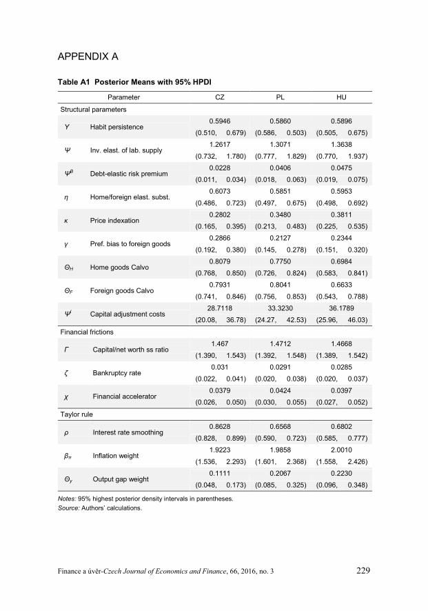
APPENDIX A Table A1 Posterior Means with 95% HPDI

Parameter CZ PL HU


Υ Habit persistence 0.5946 0.5860 0.5896

(0.510, 0.679) (0.586, 0.503) (0.505, 0.675)

Ψ Inv. elast. of lab. supply 1.2617 1.3071 1.3638

(0.732, 1.780) (0.777, 1.829) (0.770, 1.937)

ΨB Debt-elastic risk premium 0.0228 0.0406 0.0475

(0.011, 0.034) (0.018, 0.063) (0.019, 0.075)

η Home/foreign elast. subst. 0.6073 0.5851 0.5953

(0.486, 0.723) (0.497, 0.675) (0.498, 0.692)

κ Price indexation 0.2802 0.3480 0.3811

(0.165, 0.395) (0.213, 0.483) (0.225, 0.535)

γ Pref. bias to foreign goods 0.2866 0.2127 0.2344

(0.192, 0.380) (0.145, 0.278) (0.151, 0.320)

ΘH Home goods Calvo 0.8079 0.7750 0.6984

(0.768, 0.850) (0.726, 0.824) (0.583, 0.841)

ΘF Foreign goods Calvo 0.7931 0.8041 0.6633

(0.741, 0.846) (0.756, 0.853) (0.543, 0.788)

Ψl Capital adjustment costs 28.7118 33.3230 36.1789

(20.08, 36.78) (24.27, 42.53) (25.96, 46.03)

Financial frictions

Γ Capital/net worth ss ratio 1.467 1.4712 1.4668

(1.390, 1.543) (1.392, 1.548) (1.389, 1.542)

ζ Bankruptcy rate 0.031 0.0291 0.0285

(0.022, 0.041) (0.020, 0.038) (0.020, 0.037)

χ Financial accelerator 0.0379 0.0424 0.0397

(0.026, 0.050) (0.030, 0.055) (0.027, 0.052)

Taylor rule

ρ Interest rate smoothing 0.8628 0.6568 0.6802

(0.828, 0.899) (0.590, 0.723) (0.585, 0.777)

βπ Inflation weight 1.9223 1.9858 2.0010

(1.536, 2.293) (1.601, 2.368) (1.558, 2.426)

Θy Output gap weight 0.1111 0.2067 0.2230

(0.048, 0.173) (0.085, 0.325) (0.096, 0.348)

Notes: 95% highest posterior density intervals in parentheses.



Table A2 Prior Densities (Exogenous Processes)

Parameter Distribution Prior

Mean Std

Shock persistences

ρY Productivity shock B 0.5 0.2

ρUIP UIP shock B 0.5 0.2

ρLOP LOP shock B 0.5 0.2

ρNW Net worth shock B 0.5 0.2

Shock volatilities

σY Productivity shock IG 1.0 ∞

σUIP UIP shock IG 1.0 ∞

σLOP LOP shock IG 1.0 ∞

σNW Net worth shock IG 1.0 ∞

σMP Monetary policy shock IG 0.1 ∞

σy* Foreign output IG 0.5 ∞

σπ* Foreign CPI inflation IG 0.2 ∞

σi* Foreign interest rate IG 0.1 ∞

Notes: B—beta distribution, IG—inverted gamma distribution.


Prior setting of the foreign SVAR(1) block

π

ε

π π ε

ε

∗∗ ∗−

∗ ∗ ∗−

∗ ∗ ∗−

= +

1

1

1

0.8 0 0 1 0 00 0.2 0 0.5 1 00 0 0.6 0.3 0 1

yt t t

t t ti

t t t

y y

i i

(A1)

Posterior means of the Czech model

π

ε

π π ε

ε

∗∗ ∗−

∗ ∗ ∗−

∗ ∗ ∗−

−

= − + −

1

1

1

0.90 0.55 0.50 1 0 00.16 0.20 0.64 0.15 1 00.06 0.06 0.58 0.09 0.04 1

yt t t

t t ti

t t t

y y

i i

(A2)

Posterior means of the Polish model

π

ε

π π ε

ε

∗∗ ∗−

∗ ∗ ∗−

∗ ∗ ∗−

−

= − + −

1

1

1

0.89 0.48 0.49 1 0 00.13 0.20 0.51 0.16 1 00.06 0.05 0.55 0.09 0.04 1

yt t t

t t ti

t t t

y y

i i

(A3)

Posterior means of the Hungarian model

π

ε

π π ε

ε

∗∗ ∗−

∗ ∗ ∗−

∗ ∗ ∗−

−

= − + −

1

1

1

0.89 0.45 0.60 1 0 00.12 0.19 0.49 0.17 1 00.07 0.04 0.53 0.09 0.04 1

yt t t

t t ti

t t t

y y

i i

(A4)


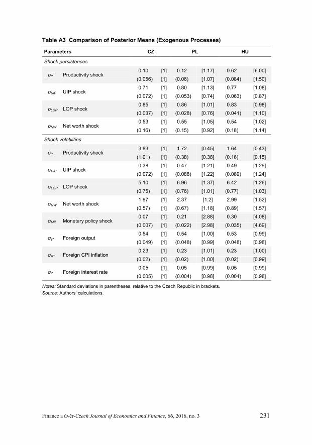
Table A3 Comparison of Posterior Means (Exogenous Processes)

Parameters CZ PL HU

Shock persistences

ρY Productivity shock 0.10 [1] 0.12 [1.17] 0.62 [6.00]

(0.056) [1] (0.06) [1.07] (0.084) [1.50]

ρUIP UIP shock 0.71 [1] 0.80 [1.13] 0.77 [1.08]

(0.072) [1] (0.053) [0.74] (0.063) [0.87]

ρLOP LOP shock 0.85 [1] 0.86 [1.01] 0.83 [0.98]

(0.037) [1] (0.028) [0.76] (0.041) [1.10]

ρNW Net worth shock 0.53 [1] 0.55 [1.05] 0.54 [1.02]

(0.16) [1] (0.15) [0.92] (0.18) [1.14]

Shock volatilities

σY Productivity shock 3.83 [1] 1.72 [0.45] 1.64 [0.43]

(1.01) [1] (0.38) [0.38] (0.16) [0.15]

σUIP UIP shock 0.38 [1] 0.47 [1.21] 0.49 [1.29]

(0.072) [1] (0.088) [1.22] (0.089) [1.24]

σLOP LOP shock 5.10 [1] 6.96 [1.37] 6.42 [1.26]

(0.75) [1] (0.76) [1.01] (0.77) [1.03]

σNW Net worth shock 1.97 [1] 2.37 [1.2] 2.99 [1.52]

(0.57) [1] (0.67) [1.18] (0.89) [1.57]

σMP Monetary policy shock 0.07 [1] 0.21 [2.88] 0.30 [4.08]

(0.007) [1] (0.022) [2.98] (0.035) [4.69]

σy* Foreign output 0.54 [1] 0.54 [1.00] 0.53 [0.99]

(0.049) [1] (0.048) [0.99] (0.048) [0.98]

σπ* Foreign CPI inflation 0.23 [1] 0.23 [1.01] 0.23 [1.00]

(0.02) [1] (0.02) [1.00] (0.02) [0.99]

σi* Foreign interest rate 0.05 [1] 0.05 [0.99] 0.05 [0.99]

(0.005) [1] (0.004) [0.98] (0.004) [0.98]

Notes: Standard deviations in parentheses, relative to the Czech Republic in brackets.



Figure A1 Time-Varying Impulse Response Functions of Real Output (CZ)

Notes: Impulse responses to 1% shocks are depicted.


Figure A2 Time-Varying Impulse Response Functions of Real Output, Crisis Period (CZ)

Notes: Impulse responses to 1% shocks are depicted, shaded area—pre-crisis period (2003Q3–2008Q2), black line—pre-crisis mean.



Figure A3 Time-Varying Impulse Response Functions of Real Output (PL)



Figure A4 Time-Varying Impulse Response Functions of Real Output, Crisis Period (PL)




Figure A5 Time-Varying Impulse Response Functions of Real Output (HU)



Figure A6 Time-Varying Impulse Response Functions of Real Output, Crisis Period (HU)




REFERENCES

Adjemian S, Bastani H, Juillard M, Karamé F, Mihoubi F, Perendia G, Pfeifer J, Ratto M, Villemot S (2011): Dynare: Reference Manual, Version 4. CEPREMAP, Dynare Working Papers, no. 1.

Bernanke BS, Gertler M, Gilchrist S (1999): The Financial Accelerator in a Quantitative Business Cycle Framework. In: Taylor JB, Woodford M (Eds.): Handbook of Macroeconomics. Vol. 1. Elsevier, Amsterdam, pp. 1341–1393.

Brooks SP, Gelman A (1998): General methods for monitoring convergence of iterative simulations. Journal of Computational and Graphical Statistics, 7(4):434–455.

Brzoza‐Brzezina M, Kolasa M (2013): Bayesian evaluation of DSGE models with financial frictions. Journal of Money, Credit and Banking, 45(8):1451–1476.

Brzoza-Brzezina M, Kolasa M, Makarski K (2013): The anatomy of standard DSGE models with financial frictions. Journal of Economic Dynamics and Control, 37(1):32–51.

Čapek J (2012): Comparison of recursive parameter estimation and non-linear filtration. In: Ramík J, Stavárek D (Eds.): Mathematical Methods in Economics 2012. Karviná, Silesian University, School of Business Administration, pp. 85–90.

Christiano LJ, Trabandt M, Walentin K (2011): Introducing Financial Frictions and Unemployment into a Small Open Economy Model. Journal of Economic Dynamics and Control, 35(12): 1999–2041.

European Central Bank (2000): EU Banks’ Margins and Credit Standards. December 2000.

Fernández-Villaverde J, Rubio-Ramírez JF (2007): How Structural are Structural Parameters? NBER Working Papers, no. 13166.

Haug AJ (2005): A Tutorial on Bayesian Estimation and Tracking Techniques Applicable to Nonlinear and Non-Gaussian Processes. MITRE corporation, Mitre Technical Report.

Justiniano A, Preston B (2006): Monetary Policy and Uncertainty in an Empirical Small Open Economy Model. Journal of Applied Econometrics, 25(1):93–128.

Kulish M, Pagan A (2013): Estimation and Solution of Models with Expectations and Structural Changes. CEPREMAP, Dynare Working Paper Series, no. 34.

Němec D (2013): Evaluating labour market flexibility in V4 countries. In: Vojáčková H (Ed.): Mathematical Methods in Economics 2013. Jihlava, College of Polytechnics Jihlava, pp. 661–666.

Ryšánek J, Tonner J, Tvrz S, Vašíček O (2012): Monetary policy implications of financial frictions in the Czech Republic. Finance a úvěr-Czech Journal of Economics and Finance, 62(5):413–429.

Shaari MH (2008): Analyzing Bank Negara Malaysia’s Behaviour in Formulating Monetary Policy: An Empirical Approach. Canberra, Australian National University, College of Business and Economics. [Doctoral thesis.]

Tamási B, Világi B (2011): Identification of credit supply shocks in a Bayesian SVAR model of the Hungary economy. MNB Working Papers, no. 2011/7.

Tvrz S (2015): Czech and Polish Experience of the Great Recession: DSGE Model Approach. In: Jedlička P (Ed.): Hradec Economic Days 2015. Hradec Králové: Gaudeamus, pp. 295–301.

Tvrz S, Vašíček O (2014): Nonlinear DSGE model of a small open economy with time-varying parameters: Czech economy in a period of recession. In: Talašová J, Stoklasa J, Talášek T (Eds.): Mathematical Methods in Economics 2014. Olomouc, Palacký University, pp. 1068–1073.

Vašíček O, Tonner J, Polanský J (2011): Parameter Drifting in a DSGE Model Estimated on Czech Data. Finance a úvěr-Czech Journal of Economics and Finance, 61(5):510–524.

the great recession in the non-emu visegrád countries: a

Documents