special relativity using perplex numbers

Research Article

2021Vol.12 No.4:16

iMedPub Journalswww.imedpub.com

1

Advances in Applied Science Research

© Under License of Creative Commons Attribution 3.0 License | This article is available in: https://www.imedpub.com/advances-in-applied-science-research/

1b

Shyamkant Anwane

Department of Physics, Shri Shivaji Education Society, Amravati's Science College, Congress Nagar, Nagpur, India

*Corresponding author: Shyamkant Anwane

[email protected]

Department of Physics, Shri Shivaji Education Society Amravati's Science College, Congress Nagar, Nagpur-440012 India.

Tel: 09422122711

Citation: Anwane SW (2021) Special Relativity using Perplex Numbers. Adv Appl Sci Res Vol. 12 No. 4:16

Special Relativity using Perplex Numbers

AbstractImaginary numbers are not merely a part of mathematical jugglery they are of relevance in the real world too. Mathematical models involving real-time and imaginary space are efficient in predicting observable effects and beyond. This research paper aims to reformulate the special relativity using perplex numbers or split complex numbers also known as hyperbolic complex numbers which mankind has been familiar with even before we knew about relativity. Hypotheses that time is real and space is imaginary offers a new look at the space-time fabric. The invariant quantities in special relativity are of hyperbolic formats. This eventually leads to hyperbolic geometry that supports the basic structure of equations. Therefore, the use of hyperbolic complex numbers or perplex numbers handles all perspectives of special relativity with elegance and offers a great degree of simplicity so that even with a meager knowledge of mathematics allows the reader to handle special relativity. The findings support the hypothesis that time is real and space is imaginary in perplexes number representation. A few applications of special relativity in the realm of Quantum Mechanics and Nuclear Physics viz Berkley Collider, Compton’s Effect, Quantum Doppler Effect have been successfully explored.

Keywords: Berkeley collider; Complex numbers; Compton's effect; energy; Perplex number; Quantum Doppler effect; Special relativity

Received: January 10, 2021; Accepted: March 11, 2021; Published: April 06, 2021

IntroductionThe complex number system is at the heart of complex analysis and has enjoyed more than 150 years of intensive development along with finding applications in diverse areas of science and engineering. Perplex Numbers are also known as Split Complex numbers or double numbers that have reported applications in explaining many concepts in Physics. Recently in 2003, Bracken and Hayes [1] reported an effective use of perplex numbers for Klein-Gordon equation.

At the beginning of the Twentieth Century, Albert Einstein [2] developed his theory of special relativity, built upon Lorentzian geometry, yet at the end of the century, almost all high school and undergraduate students were still taught only Euclidean geometry. Partly, the reason for this state of affairs has been the lack of simple mathematical formalism in which the basic ideas can be expressed. This research paper claims the formulation of special relativity in perplex numbers configuration that proficiently encompasses the subject elegantly and its consequences with profound simplicity. However, in literature, we find wide reporting of the use of perplex numbers or split complex numbers or hyperbolic geometry concepts for Special Relativity [3-6]. Although the use of perplex numbers is not

innovative in this era, the present work attempts to prove the advantage of novel definitions using perplex numbers. Lorentz transformation equations are configured in terms of a single perplex equation. This research paper proposes new definitions of perplex kinematic parameters and its consequent exploration by proper time differentiations and complex conjugate multiplication. New tools are also defined using perplex numbers. Moreover, the proposed approach offers the simplest possible descent to relativistic energy equation while it preserves all consequences of relativity. A couple of applications of SR in the realm of Quantum Mechanics and Nuclear Physics have been are explored for testing the validity as hands-on experience testing the validity of proposed new approach of Special Relativity using Perplex Numbers.

Theory and ExperimentationDefinitionsPerplex Numbers also known as Split Complex numbers or double numbers possess two real components x and y and written in ordered pair as (x,y) where 1j = − unlike 1i = − .

0 1( , )z x yj x y xe ye= + = = + …… (1)

2021Vol.12 No.4:16

2


This article is available from: https://www.imedpub.com/advances-in-applied-science-research/

And its conjugate is defined as;*

0 1( , )z x yj x y xe ye= − = − = − …… (2)

Its unit basis vectors in determinants form may be written as;

0 1

1 0 0 1,

0 1 1 0e e = =

…….. (3)

,a b

zb a

=

* a b

zb a

− = −

…….. (4)

The obvious properties of these basis vectors are;

0 0 0 0 1 1 0 12 21 0 0 1

,1, | | 1,| | 1

e e e e e e e ee e j e e j

= = == = = = = − =

….. (5)

Here, e_0 is 2×2 unit matrix (I). A perplex number and conjugate of another number may be expressed as;

*1 0 1 2 0 1,z ae be z ce de= + = − ……. (6)

Product of such a pair is an entity of special physical significance, which may be defined in general as follows;

( ) ( )*3 1 2 0 1z z z ac bd e bc ad e= = − + − …… (7)

Moreover, the self product of a perplex number may be used to express length of that number. In perplex numbers, 1| |z may be regarded as length of the perplex number which can be used for

analogous Euler’s representation for 1tanh ba

φ −= as following;

* 21 1 1 0

* 2 2 11 1 1 1 1

| || | , | | , | | , tanh /j j

z z z ez z e z z e z a b b aφ φ φ− −

== = = − =

…… (8)

The collection D of all complex numbers : ,z x yj x y R= + ∈ (where 2 1j = ), forms an algebra over the field of real numbers. The two perplex numbers 1z and 1z have product 1z 2z that

satisfies 1 2 1 2( ) ( ) ( )N z z N z N z= . Similar algebra based on square

and component-wise operations of addition; multiplication offers a quadratic form over 2R . The ring isomorphism;

2 : ( , )D R x yj x y x y→ + + −

relates proportional quadratic forms but mapping is not isometric. The multiplicative inverse of a perplex number 1z may be denoted as 1

1z− may be expressed as follows;

11 1 0z z e− = ….. (9)

to obey relationship 11 1 0z z e− = which is a unit matrix, provided

1| | 0z ≠ .

Event in Perplex numbers (Z)To explore the quantities of Special Relativity using Split Complex Numbers, we shall substitute a ct= and b r= for defining an event or space-time position Z. In fact, we propose hypothesis that time is real and space is imaginary in perplex number or split complex numbers representation. Here, we differ with the idea mentioned by Carbajal wherein time is considered as an imaginary quantity [7]. Similarly, an offbeat reporting is also found in the literature where the speed of light is treated imaginary by Mehran Rezaei [8].

We now propose to represent time and space using perplex numbers as;

( ) ( )1 2* *, , , j jct r ct rZ ct r e Z ct r Z e

r ctZ

r ct∅ ∅−

= = = = − = = − …… (10)

where; 2 2 2 * 1 11 2| | | |, tanh , tanhr rZ c t r Z

ct ctφ φ− − −

= − = = = Now, the

modulus or length of Z denoted by Z may be expressed as;

( )* * 2 2 2| | | | | |ZZ Z Z c t r= = = − …….. (11)

Where, the product of perplex number and its conjugate *ZZdepicted in equation over matrix multiplication appears as;

2 2 2*

0ct r ct r c t r

ZZr ct r ct

− − = = −

…… (12)

Here r/t resembles velocity u of the material object which ranges of 0..c confining the term relative velocity u/c ranging over 0..1. Figure 1 depicts variation of Euler angle φ as a function of relative velocity u/c over possible range from 0 to 1. Moreover, Figure 2 depicts a cone that represents present universe cone along with the grid lines that is composed of hyperbolic curves

2 2 2 2 20, 1 , 2 ,...c t r− = ± ± and by a horizontal line inclined at angles 0, 0.25, 0.50, 0.75, 0.99.φ = ± ± ± ± . The stationary objects will be

represented by a horizontal line having 0° angle to x-axis or say

Figure 1 Variation of Euler angle ϕ as a function of relative velocity β.

2021Vol.12 No.4:16

3© Under License of Creative Commons Attribution 3.0 License


t-axis c = 1 . The moving objects are represented by inclined lines bearing angle φ that is ranging over 0 45o− . The fastest propagation represented by v = c is by the line inclined at 45o . The uncharted carpet in the plane is absolutely separated. Thus, we have a perplex environment that offers a quantity called modulus or length of a perplex numbers that is Lorentz Invariant

i.e., * * 2 2 2| | | | ZZZ Z c t r= = = − which is defined in relativity as the interval in the space-time continuum. This is a fascinating form of perplex numbers as all inertial observers agree upon this quantity making this number universal. The product *ZZ possesses only real part that is determined by the determinant of *Z or *Z which we regard in terms of length of perplex number. Note that the

associated component is the Euler angle 1tanh uc

φ −= that makes

its description 1tanh uc

φ −= complete and meaningful.

The significance of the Euler’s angle 1tanh rct

φ − =

in the event can be understood as following:

When ct > r the event is time-like 0 1rct

< < UNIVERSE

When ct > r the event is space-like 1 rct

∞< < REMOTE

When ct > r the event is light-like 0 1rct

< = path of em radiation

Note that: ct r ctr ct r

=

is a shorthand way of expressing

perplexes number without the loss of generality.

Lorentz transformation as a Perplex number

From Special Relativity we know the Lorentz Transformation equations ( )'ct ct rγ β= − and ( )'r r ctγ β= − . We can explore matrix representation to express it as;

''

ct ctr r

γ βγβγ γ

− = −

…… (13)

The Lorentz Transformation is a perplex number and in matrix form it can be expressed as;

1 *,LT LT LTγ βγ γ βγβγ γ βγ γ

−− = = = −

…… (14)

The above equation of Lorentz transformation is also a perplex number and can be expressed in the ordered pair as ( ),LT γ βγ= −

. The complex conjugate of this Lorentz Transformation perplex number ( )1 * ,LTLT γ βγ− = = can be regarded as Inverse Lorentz Transformation. Obviously, when perplex number multiplied with its conjugate offers unity.

*0.LT LT e

γ βγ γ βγβγ γ βγ γ

− = = −

….. (15)

Moreover, it is worth mentioning here that the matrix operator - Lorentz Transformation offers number length unity which in fact keeps the perplex numbers unaltered over multiplication;

*| | 1 | |LT LT= = . Thus, the Lorentz invariance in Special Relativity can be re-looked in perplex numbers easily as the perplex number multiplied by unity. However, it offers a new perplex complex number with same modulus but different Euler’s angle for another inertial observer.

1tanh1 1j jLT e e β−− Φ −= × = × ……. (16)

If one desires to speak in terms of hyperbolic angle the

trigonometric identity 2 2 22

1cosh sinh 1 cosh1 tanh

Φ − Φ = ⇒ Φ =− Φ

offers us (i) tanh βΦ = (ii) cosh γΦ = and (iii) sinh βγΦ = . It

offers geometric version of Lorentz Transformation equation as

tanhφ β= as following:

' cosh sinh' sinh cosh

ct ctr r

Φ − Φ = − Φ Φ

……. (17)

cosh sinhsinh cosh

jLT e− ΦΦ − Φ = = − Φ Φ

is also a perplex number like

equation (1) and thus we have cosh sinhje j− Φ = Φ − Φ that represents in fact the Lorentz boost. Thus, the Euler’s like identity in perplex numbers offers us an elegant Lorentz Transformation equation and its inverse as;

1 1' 'tanh tanh' 'Z' | ' | , '

r rj jct ctZ e Z e Z

− − − = =

……. (18)

for obvious notation ' cosh ' sinh 'je jφ φ φ= + and the hyperbolic

angle 1 '' tanh'

rct

φ − =

. The quantities of transformed perplex

numbers bears following identities.

'' '

jc t r r c t

Z Z er c t c t rγ βγ γ β γγ β γ γ βγ

∅− − = = − −

……… (19)

Interpretation of | |LT : After exercising | |LT on | |Z we obtain

| ' |Z and 'φ .

( ) ( )2 2 2 2 2| ' |Z c t r r c t c t rγ β γ γ β γ= − − − = − …….. (20)

This offers us an important conclusion regarding invariance of relativistic interval as following;

Figure 2 Euler like identity offering ϕ=constant and 2 2t r constant− = considering c=1 to depict space-

time warp.

2021Vol.12 No.4:16

4



* * 2 2 2| | | | | ' | | ' |Z Z Z Z c t r= = = = − ……. (21)

Interpretation of 'φ : The Euler’s angular component

1 1tanh tanhr uct c

φ − −= = for rut

= . Now for 'φ we can write;

1 1' ' '' tanh tanh , '' '

r u ruct c t

φ − −= = = …….. (22)

From equation (19) re-write 1tanh 'φ− in the last equation as;

2

'' 1

r vr r c t trvct c t r cc t

γ β γγ β γ

−−= =

− −

……. (23)

Substituting '' rut

= and '' rut

= in the last equation, we get

2

'1

u vu uvc

−=

− …….. (24)

Now, exercising inverse Lorenz transformation 1* tanh1 jLT e β−+= ×

on event Z will offers us the same formula for modulus as in the

equation (21). While the Euler angle is on the similar lines of

equation (24) with a difference of sign as;

2

'1

u vu uvc

+=

+ ……(25)

The above equation (25) is the Composition of Velocity in Special Relativity. We shall revisit Composition of Velocity in Article 6 separately as a consequence of Lorentz boost to to develop consequences of Perplex Number Special Relativity.

Geometrical Interpretation of 'φ : The Lorentz transformation in Euler’s form;

'' . | ' | | |j j jZ LT Z Z e e Z eφ φ− Φ= ⇒ = ….. (26)

As | ' | | |Z Z= we have;

' 'φ φ φ φ= −Φ ⇒ = +Φ …… (27)

Operating 1tanh− on both sides and substituting

( )1 1

11 1

tanh ' tanhtanh '1 tanh 'tanh

φφφ

− −−

− −

+ Φ+Φ =

+ Φ.

2 2

''

' '1 1

u vu u vc c uu v u vc

c c

+ += ⇒ =

+ + ….. (28)

Thus, we arrive at the velocity composition through the addition of the hyperbolic angle.

Relativistic Kinematics using Perplex Numbers

To establish kinematics of Special Relativity as developed by

Landau and Lifshitzs [9,10] in terms 4-vectors of perplex numbers. Consider an event represented in frame S and S’ which forms a pair of inertial frames with all usual contentions and arguments established in the subject. An event or perplex position can be represented by Z ct rj= + and dZ cdt drj= + which are related by Lorentz Transformation equation (13). By definition, an infinitesimal interval which in another words is length of perplex numbers is invariant for all inertial observers. We have dZ cdt drj= + and ' ' 'dZ cdt dr j= + .

| | | ' |dZ dZ= …… (29)

Now we impose that the event occurs at the origin of the coordinate system so that

't. This will simplify the last

equation as;2 2 2 2 2'c dt dr c dt− =

Changing over notation 't to τ and substituting / ( )dr dt v t= , ( ) /t v cβ = and 21 / 1γ β= − and simplifying we get;

2

11

dtd

γτ β= =

− …… (30)

Thus, the Lorentz factor γ represents the rate at which time t changes with respect to proper time v . Here v is regarded as relative velocity between two inertial frames S and S’.

Position ( Z ) using Perplex Numbers: The relativistic event can be expressed in perplex number space-time representation as in (10) its complex conjugate can be expressed as (11) while its modulus can be expressed as (12). Note that: The Lorent transformation equation may be written as ' .Z LT Z= and it yields Lorentz invariance for the quantity ( )2* * 2 2 2| ' ' | | |Z Z ZZ c t r= = − and 1' tanh ( ' / )u cφ −= .

Velocity ( ) using Perplex Numbers: We shall define perplex velocity by differentiating perplex position with respect to the proper time which is a universal quantity for all inertial observers.

( )dZ dV ct rjd dτ τ

= = + ……. (31)

Substituting /dt dτ γ= and / /dr d dr dt vτ γ γ= = , we get;

( ) 12ã jtanhc vV c vj c e

v cβγ γ

γ γ−

= + = =

…… (32)

Note that here v is the usual velocity by definition. The varied forms in which the Velocity using perplex number or simply perplex velocity may be written are as follows;

( ) 1* 2ã jtanhc vV c vj c e

v cβγ γ

γ γ−−−

= − = = − …… (33)

Its conjugate ( )* cV c vj

cγ

γβγ

= − = −

on multiplication with V

offers an invariant quantity or length of perplex number 2c as

depicted below.

2*

2

0

0c

VVc

=

……. (34)

2021Vol.12 No.4:16



' . c v

V LT Vv c

γ βγ γ γβγ γ γ γ

− − = = − −

…….(35)

' 00c

cV

=

..….(36)

Note that: The Lorentz transformation equation may be written as ' .V LT V= and it yields Lorentz invariance * * 4| ' ' | | |V V VV c= = . Thus, operating unit length perplex number LT retains the length of the perplex number on which it is operated i.e., perplex velocity. The invariance governing equation 2| | | ' |V V c= = is same for all inertial observers which are in fact the universal constant.

Momentum ( P ) using Perplex numbers: We shall define perplex momentum by multiplying mass (a scalar number) with perplex velocity.

10 00

0 0

| | jcm vmP m V P e

vm cmγ γγ γ

∅ = = =

….(37)

10 0* * *0

0 0

| | jcm vmP m V P e

vm cmγ γγ γ

− ∅− = = = −

…. (38)

* * 2 2 10 1| | | | | | , tanhPP P P m c PPφ β−= = = = ….. (39)

Its conjugate *P on multiplication with P offers an invariant quantity or length of perplex number 2 2

0m c . Here m0 is proper mass which is an essentially universal quantity that all inertial observers can agree upon and ym0 = m;

* , mc mv mc mv

P Pmv mc mv mc

− = = −

…. (40)

The varied forms in which the momentum using perplex number or simply perplex momentum may be written are as follows;

2 2* * , j j

E Ep pc cP P e P P e

E Ep pc c

∅ − ∅

− = = = = −

…. (41)

Here, in the last equation we propose to rewrite the perplex momentum equation (39) wherein the real part /mc E c= is abstract of Einstein’s most famous equation 2E mc= and imaginary part mv is usual relativistic momentum p. The complex conjugate multiplication now offers us a form as below;

22 2 20 1 2| | ,E pcm c P p

c Eφ φ β = = − = ⇒ =

………….(42)

Comparing *| |, | |P P and 1 2,φ φ from equations (39) and (42)

followed by few steps of simplification, we get the expression for relativistic energy of a particle as;

2 2 2 4 20 ,E p c m c E mc= + = ….. (43)

Note that: The Lorentz transformation equation may be written as ' .P LT P= and it yields Lorentz invariance * *' ' , | | 1P P PP LT= = .

The obvious relationship governing Lorentz transformation is as follows:

' / /'

'E c E c

Pp p

γ βγβγ γ

− = = −

…. (44)

1 /2 tanh2 /

2

/'

/

p E cjE c pE c p EP p e

p E c c

ββγ γ

γ βγ

− −−−

= = − − … (45)

0

0

' .m c

P LT Pm vγγ βγγβγ γ

− = = − …… (46)

Similarly, we can write;

10 2 2 tanh 00'

0jm c

P m c e−

= =

…. (47)

While the perplex momentum ( ) is expanded form appears as follows.

0 02 2

2 2

0 02 2

2 2

1 1

1 1

m c m vv vc cP

m v m cv vc c

− − = − −

…. (48)

In above equation we have used a substitution

( )1

2 2 20 0 1 /m c m c v cγ

−= − on binomial expansion and

simplification gives 20 0 0

1 12

m c m c m vc

γ = + . Adjusting to look

for rest energy and kinetic energy we have following equation.

2 2 20 0

12

E mc m c m v= = + ….. (49)

Acceleration ( A ) using Perplex numbers: We shall define perplex acceleration by differentiating perplex velocity with respect to the proper time (τ ).

( )dV dA c vjd d

γτ τ

= = + …. (50)

Substituting /dt dτ γ= and / /d d d dtτ γ= , we get:

( )A c v a jγ γ γ γ= + + …… (51)

Note that here a is the usual acceleration by definition and γ is time derivative of γ . The varied forms in which the Acceleration using perplex number may be written are as follows:

( )2

2ã , c v a

A c v av a cγ γ γ γ γ

γ γ γγ γ γ γ γ +

= + = +

….. (52)

The above may be further simplified after substituting the identity 3 /a cγ β γ= and its simplification take following form;

2021Vol.12 No.4:16

6



14 4

4 4 | | jtanha aA A e

a aβ γ γγ β γ

− ∅ = =

…. (53)

A little mathematical exploration will enable to arrive at following invariant quantities like other pairs ( * *, ,ZZ VV and *PP ) offered are new findings.

* * 2 6 1 1| | | | | | , tanhA A AA a γ φβ

−= = = − = ….. (54)

Note that: The Lorent transformation equation may be written as ' .A LT A= and to yield Lorentz invariance

( )2* * 2 6' 'A A AA a γ= = . We shall explore perplex acceleration under Lorentz Transformation equation.

2'c

Av a

γ βγ γγβγ γ γγ γ

− = − +

2 5 5

2 5 5

0 a'

a 0a

Aa

β γ γβ γ γ

− += − +

…. (55)

Thus, the above discussion yields out information regarding acceleration in perplex numbers and length of perplex acceleration that remains invariant under Lorentz Transformation is 2 6| | | ' |A A a γ= = − and 1tanhφ ∞−= .

Force ( F ) using Perplex numbers: We shall define perplex force by differentiating perplex momentum with respect to the proper time (τ ).

( )0 0dP dF m c m vjd d

γ γτ τ

= = + …… (56)

Substituting /dt dτ γ= and / /d d d dtτ γ= , we get:

( )20 0 0F m c m v m a jγ γ γ γ γ = + + (57)

Note that here is the usual acceleration by definition and time derivative of bearing relationship . The varied forms in which the Force using perplex number or simply perplex force may be written are as follows:

…. (58)

Here, ( )230| |F m aγ= and 1/φ β= leads to the Euler’s form of

Perplex force.

( ) ( )1 12 23 tanh 1/ * 3 tanh 1/0 0,j jF m a e F m a eβ βγ γ

− − −= = ….. (59)

Note that: The Lorent transformation equation may be written as ' .F LT F= but is is observed that it disobeys Lorentz invariance

for Newtonian Force | | | ' |F F= and * *' 'F F FF= . To express it more obviously we shall explore perplex force under Lorentz Transformation equation.

4 40 0

4 40 0

'm a m a

Fm a m a

γ βγ βγ γβγ γ γ βγ

− = −

….. (60)

On solving the product and exploring simplification, we get;

30

30

0'

0m a

Fm a

γγ

=

….. (61)

Thus, the above discussion yields out information regards force in perplex numbers and length of perplex acceleration that remains invariant under Lorentz Transformation. Thus, we conclude following:

( )2* * * 30| | | | | ' | | ' | | ' |F F F F FF m aγ= = = = = − …. (62)

From equation (62) we can write Euler’s form as;

( )23 10' , tanhF m aγ φ ∞−= − = ….. (63)

Another Approach: Combining equations (41) and (56) we can re-assemble another from for equation as;

ã

E pd cF

Edt pc

=

……. (64)

From mechanics we know 0/ 'dE dt fv m a v= = and 0/ 'dp dt m a=, we get;

1' '

' 20 00' '

0 0

( ) tanhm a m aF m a e

m a m aβγ γγ βγ

− ∞ = =−

….. (65)

The Lorentz transformation of above equation on simplification offers following form along with its Euler’s representation;

1'

' ' 200'

0

0. ( )

0tanhm a

F LT F m a em a

− ∞ −= = = −

….. (66)

Now comparing equations (66) and (63) we can conclude following.

3'a aγ= …. (67)

This is in agreement with the findings of acceleration by Rindler [11-13] in 1966.

Velocity composition

Let an observer A is in an inertial frame measures space-time coordinates of an event as; ( , )Z ct r= . Another inertial observer B (say in frame S’) records the same event denoted as ' ( ', ')Z ct r= is moving with relative velocity 1 1 /v cβ = with respect to observer A (i.e., frame S). The concerned hyperbolic angle in analogous Euler’s representation be 1φ . Now let us consider the third observer C is moving with relative velocity 2 2 /v cβ = with respect to observer B (say frame S’). The concerned hyperbolic angle be 2φ . Now, with respect to A, let the resultant relative

2021Vol.12 No.4:16



velocity be /v cβ = and the concerned hyperbolic angle, say will obviously be the sum of the first two angles 1 2φ φ φ= + .

( ) 1 21 2

1 2

tanh tanhtanh1 tanh tanh

φ φφ φφ φ±

± =±

….. (68)

But for the definition, we know; 1 1 2 2tanh , tanh , tanhφ β φ β φ β= = = which leads to the manner in which relative velocities can be added.

1 2

1 21β βββ β+

=+

…. (69)

The above equation is consistent with findings of Einstein’s Special Relativity [2,10].

Consequences of Lorentz boost

Let a pair of events charts with a complex number be expressed as 1 1 1Z ct r j= + and 2 2 2Z ct r j= + in frame S . Now we shall look for the effect of Lorentz boost to offer a look at view of a observer moving with uniform velocity along -axis referred as an inertial frame 'S . The same pair of events may be chart with a complex number be expressed as 1 1' .Z LT Z= and 2 2' .Z LT Z= in frame 'S . The observer in 'S measures interval between two events as

2 1' ' 'dZ Z Z= − .

' .dZ LT dZ= …. (70)

The explicit expanded form of the above equation looks as follows:

cd cdtd drτ γ βγλ βγ γ

− = −

…. (71)

Comparing real and imaginary parts we get following pair of equations which we are interested in exploring.

( )( )

cd cdt drd dr cdtτ γ βλ γ β= += −

….. (72)

The time dilation: Let the two events occur at same location 0dr = and differ only in time (real part). For example, a flash of

light occurring at same place after a time interval. Comparing real-part of the last equation (72) and simplifying for 0dr = for real part, we get:

d dtτ γ= ….. (73)

This relation (73) depicts time dilation suggested by Einstein’s Special Relativity [2,10].

The space contraction: Let the two events occur at time location 0dt = and differ only in space location dr. For example, measuring

length of a rod at a moment of time. Comparing imaginary-part of the last equation (72) and simplifying for 0dt = , we get:

d drλ γ= ….. (74)

Let the two events occur at same time and differ only in space location which is imaginary part in complex number representation of events. Let the observer in frame S’ measure

length that is stationary relative to the rod. Hence, we define this length as a proper length 0d lλ = . The rod moving parallel to its length will appear of length ( )dr l v= given by expression:

( ) oll vγ

= …. (75)

The above relation (25) depicts length contraction as suggested by Einstein’s Special Relativity [2,10].

Simultaneity is relative: Now we shall deal with the issue of simultaneity in special relativity. We shall again explore pair of equations (72) and per-conceive that two events are occurring at two different spatial locations and are simultaneous in frame S . Imposing 0dr ≠ and 0dr ≠ , we get

cd cdrd drτ γβλ γ==

…. (76)

For this event to be simultaneous in frame 'S , i.e., 0dr = it is essential that 0dr = . It means that two events simultaneous in one inertial frame does not guarantee that it will be simultaneous for other inertial observers. For absoluteness of simultaneity, the event should not only be simultaneous in one frame but also must occur at the same location.

Velocity in moving frame: To add velocities together, consider a physical situation accordingly.

1 *'dZ LT dZ LT dZ−= = …. (77)

The explicit expanded form of the above equation looks as follows:

cd cdtd drτ γ βγλ βγ γ

=

…. (78)

Comparing real and imaginary parts we get following pair of equations which we are interested in exploring.

( )( )

cd cdt drd dr cdtτ γ βλ γ β= += +

…. (79)

Consider ratio of latter to the former equation in the last

equation (79), with substitutions; '( ) /u d dτ λ τ= is velocity in

frame 'S , ( ) /u t dr dt= is velocity in frame S :

2

( )'( ) ( )1

u t vu u t vc

τ ±=

± ….. (80)

Thus, perplex numbers offer the velocity addition formula by another approach also. Another version for subtracting velocities can also be raised from the analogous equation; ' .dZ LT dZ= that offers us another equation depicted in equation (80) with minus sign.

Acceleration in a moving frame

Differentiating one of the equations (80) with respect to and exploring the equation (30)

2021Vol.12 No.4:16

8



2

( )'( ) ( )1

d d u t vu u t vd dtc

τ γτ

−

= −

…. (81)

Substituting ' '( ), ( )d da u a u td dt

ττ

= = , d dd dt

γτ= and simplifying

we get:

2

2

'( )( )1

aau t v

c

τγ

= −

….. (82)

For slow speed considerations we can employ 2( )u t v v≈ and induct γ accordingly to further simplify the equation:

3'a γ= …. (83)

Acceleration leading to Rindler space

We have established acceleration in moving frame as 3aγ which on comparison with the spatial component of acceleration arising from equations (52) offers us:

2 3v a aγγ γ γ+ =

….. (84)

The above equation (84) resembles acceleration leading to Rindler space [12-16]. Note that 0 1A a a j= + wherein we refer

0a as temporal and 1a as spatial components. Simplifying the last equation and replugging derivative notations to look for the differential equation version, we get:

2v v vγ γ γ+ = …. (85)

The above equation leads to the Rindler space on the line of traditional equation here aroused from the perplex acceleration component. The equation (63) may further be modified in reference to the last equation (85) as follows:

4 2 4 20 0 0

2 4 2 40 0 0

m a m a m a

Fm a m a m aβγ β γ γ

β γ γ βγ +

= + …. (86)

The Euler’s form of above equation is;

( )1 12tanh 3 tanh 1/0| | j jF F e m a eφ βγ

− −

= = −

Applications of Perplex numbers

With minimal mathematical resources, we can quickly apply the quantities raised for a couple of well-known Special Relativity applications to try hands-on with perplex numbers.

A free electron cannot absorb a photon: The perplex momentum

of free electron at rest can be expressed as; 0 0 10restp m ce e= + .

Note that the Lorentz factor 1γ = for electron at rest. We shall

define perplex momentum for a photon as 0 1K' h he e

c cν ν

= + .

,| | 0

h hc cK K

h hc c

ν ν

ν ν

= =

…. (87)

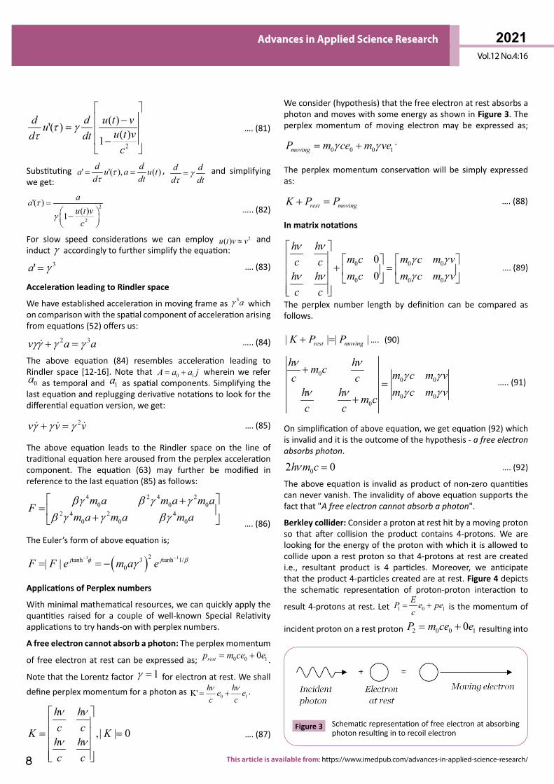
We consider (hypothesis) that the free electron at rest absorbs a photon and moves with some energy as shown in Figure 3. The perplex momentum of moving electron may be expressed as;

0 0 0 1movingP m ce m veγ γ= + .

The perplex momentum conservation will be simply expressed as:

rest movingK P P+ = …. (88)

In matrix notations

0 0 0

0 0 0

00

h hm c m c m vc cm c m c m vh h

c c

ν νγ γγ γν ν

+ =

…. (89)

The perplex number length by definition can be compared as follows.

| | | |rest movingK P P+ = …. (90)

00 0

0 00

h hm c m c m vc cm c m vh h m c

c c

ν νγ γγ γν ν

+=

+

….. (91)

On simplification of above equation, we get equation (92) which is invalid and it is the outcome of the hypothesis - a free electron absorbs photon.

02 0h m cν = …. (92)

The above equation is invalid as product of non-zero quantities can never vanish. The invalidity of above equation supports the fact that "A free electron cannot absorb a photon".

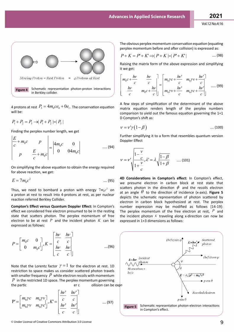
Berkley collider: Consider a proton at rest hit by a moving proton so that after collision the product contains 4-protons. We are looking for the energy of the proton with which it is allowed to collide upon a rest proton so that 4-protons at rest are created i.e., resultant product is 4 particles. Moreover, we anticipate that the product 4-particles created are at rest. Figure 4 depicts the schematic representation of proton-proton interaction to

result 4-protons at rest. Let 1 0 1EP e pec

= + is the momentum of

incident proton on a rest proton 2 0 0 10P m ce e= + resulting into

Figure 3 Schematic representation of free electron at absorbing photon resulting in to recoil electron

2021Vol.12 No.4:16



4 protons at rest 3 0 0 14 0P m ce e= + . The conservation equation will be:

1 2 3 1 2 3| | | |P P P P P P+ = → + =

Finding the perplex number length, we get

00

00

4 00 04

E m c p m ccm cEp m c

c

+=

+

….. (94)

On simplifying the above equation to obtain the energy required for above reaction, we get:

207E m c= …. (95)

Thus, we need to bombard a proton with energy 207m c on

a proton at rest to result into 4-protons at rest, as per nuclear reaction referred Berkley Collider.

Compton’s Effect versus Quantum Doppler Effect: In Compton’s effect we considered free electron presumed to be in the resting state that scatters photon. The perplex momentum of free electron to be at rest P and the incident photon K can be expressed as follows:

0

0

0,

0

h hm c c cP K

m c h hc c

ν ν

ν ν

= =

….(96)

Note that the Lorentz factor 1γ = for the electron at rest. 1D restriction to space makes us consider scattered photon travels with smaller frequency p while electron recoils with momentum p in the restricted 1D space. The perplex momentum governing

the particles after collision can be expressed as

0 0

0 0

' '

P' , '' '

h hm c m v c cKm v m c h h

c c

ν νγ γγ γ ν ν

= =

…. (97)

The obvious perplex momentum conservation equation (equating perplex momentum before and after collision) is expressed as:

' ' | | | ' ' |P K P K P K P K+ = + ⇒ + = + …. (98)

Raising the matrix form of the above expression and simplifying it we get:

0 0 0

0 0 0

' '

' '

h h h hm c m c m vc c c c

h h h hm c m v m cc c c c

ν ν ν νγ γ

ν ν ν νγ γ

+ + + =

+ + +

….. (99)

A few steps of simplification of the determinant of the above matrix equation renders length of the perplex numbers comparison to yield out the famous equation governing the 1+1 D Compton’s shift as:

( )' 1ν ν γ β= − …. (100)

Further simplifying it to a form that resembles quantum version Doppler Effect

1 1' , '11

vcvc

βν ν λ λβ

− −= =

++ ….. (101)

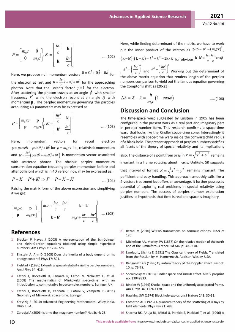
4D Considerations in Compton’s effect: In Compton’s effect, we presume electron in carbon block at rest state that scatters photon in the direction φ and the recoils electron at an angle θ to the direction of incidence (x-axis). Figure 5 depicts the schematic representation of photon scattered by electron in carbon block hypothesized at rest. The perplex number expression may be modified as follows [14-19]: The perplex momentum of the free electron at rest, P and the incident photon K traveling along x-direction can now be expressed in 1+3 dimensions as follows:

Figure 4 Schematic representation photon-proton interactions in Berkley collider.

Figure 5 Schematic representation photon-electron interactions in Compton’s effect.

2021Vol.12 No.4:16

10



0

0

0,

0

hm c cP K

m c hc

ν

ν

= =

k

k …..(102)

Here, we propose null momentum vectors 0 0 0 ˆˆ ˆ 0i j k= + + for

the electron at rest and 0 ˆˆ ˆ0h i j kcν

= + +k for the approaching photon. Note that the Lorentz factor 1γ = for the electron. After scattering the photon travels at an angle φ with smaller frequency 'ν while the electron recoils at an angle θ with momentum p . The perplex momentum governing the particles accounting 4D parameters may be expressed as:

0

0

' '' , '

''

hm c cP K

m c hc

νγ

γ ν

= =

kpp k ….. (103)

Here, momentum vectors for recoil electron

cos sin 0 ˆˆ ˆp i p j kθ θ= + +p for 0p m vγ= i.e., relativistic momentum

and ( )ˆˆ ˆ'' cos sin 0h i j kcν θ θ= + +k is momentum vector associated

with scattered photon. The obvious perplex momentum conservation equation (equating perplex momentum before and after collision) which is in 4D version now may be expressed as:

' ' ' 'P K P K P P K K+ = + ⇒ = + − …. (104)

Raising the matrix form of the above expression and simplifying it we get:

00

00

' '

''

h hm cm c c cm c h hm c

c c

ν νγ

γ ν ν

+ − − =

− + −

k kpp k k

….. (105)

Here, while finding determinant of the matrix, we have to work

out the inner product of the vectors as ( )220p m vγ⋅ = =p p ,

( ) ( ) 2 2' ' ' 2 'k k− ⋅ − = + − ⋅k k k k k k for obvious '' cosh h

c cν ν φ⋅ =k k

,

22 hk

cν =

and

22 '' hk

cν =

Working out the determinant of the above matrix equation that renders length of the perplex numbers comparison to yield out the famous equation governing the Compton’s shift as [20-23]:

( )0

' 1 coshm c

λ λ λ φ∆ = − = − ….. (106)

Discussion and ConclusionThe time-space warp suggested by Einstein in 1905 has been configured in the present work as a real part and imaginary part in perplex number form. This research confirms a space-time warp that looks like the Rindler space-time cone. Interestingly it resembles with space-time warp inside the Schwarzschild radius of a black-hole. The present approach of perplex numbers satisfies all facets of the theory of special relativity and its implications

also. The distance of a point from or ig in 2 2r x y= + remains

invariant in a frame rotating about -axis. Unlikely, SR suggests

that interval of format 2 2S x y= − remains invariant. The

pefficient and easy handling. This approach smoothly sails like a 4-vectors treatment but offers an advantage. It further possesses potential of exploring real problems in special relativity using perplex numbers. The success of perplex number exploration justifies its hypothesis that time is real and space is imaginary.

References1 Bracken P, Hayes J (2003) A representation of the Schrödinger

and Klein–Gordon equations obtained using simple hyperbolic numbers. Am J Phys 71: 726-728.

2 Einstein A, Ann D (1905) Does the inertia of a body depend on its energy content? Phys 17: 891.

3 Fjelstad P (1986) Extending special relativity via the perplex numbers. Am J Phys 54: 416.

4 Catoni F, Boccaletti D, Cannata R, Catoni V, Nichelatti E, et al. (2008) The mathematics of Minkowski space-time: with an introduction to commutative hypercomplex numbers. Springer, UK.

5 Catoni F, Boccaletti D, Cannata R, Catoni V, Zampetti P (2011) Geometry of Minkowski space-time. Springer.

6 Kreyszig E (2010) Advanced Engineering Mathematics. Wiley-India, Ohio, USA.

7 Carbajal A (2006) Is time the imaginary number? Nat Sci 4: 23.

8 Rezaei M (2010) WSEAS transactions on communications. IRAN 2: 120.

9 Michelson AA, Morley EW (1887) On the relative motion of the earth and of the luminiferous ether. Sid M6. p: 306-310.

10 Landau L, Lifshitz E (1951) The Classical theory of Fields. Translated from the Russian by M. Hamermesh. Addison-Wesley, USA.

11 Ranganath GS (1996) Quantum theory of the Doppler effect. Reso 1: 10. p: 76-78.

12 Socolovsky M (2013) Rindler space and Unruh effect. ARXIV preprint no. 13042833.

13 Rindler W (1966) Kruskal space and the uniformly accelerated frame. Am J Phys 34: 1174-1178.

14 Hawking SW (1974) Black hole explosions? Nature 248: 30-31.

15 Compton AH (1923) A quantum theory of the scattering of X-rays by light elements. Phys Rev 21: 483.

16 Sharma BK, Ahuja BL, Mittal U, Perkkio S, Paakkari T, et al. (1996) A

2021Vol.12 No.4:16



compton profile study of tantalum. Pramana J Phy 46: 289-298.

17 Tolman RC (1939) Static Solutions of Einstein's Field Equations for Spheres of Fluid. Phys Rev 55:364.

18 Fronsdal C (1959) Completion and Embedding of the Schwarzschild Solution. Phys Rev 116: 3.

19 Padmanabhan T (2009) Snippets of physics. Reso 14: 259-271.

20 Rezvani F, Shojaei MR (2018) Relativistic effects in the study of weakly

bound Be nuclei. Pramana J Phy 90: 1-8.

21 Komathiraj K, Sharma R (2018) A family of solutions to the Einstein–Maxwell system of equations describing relativistic charged fluid spheres. Pramana J Phy 90: 1-11.

22 Das PC, Murthy GS, Deshmukh PC, Venkatesh TA (2004) The real effects of pseudo forces. Reso 9, pp: 74-85.

23 Bahrami M, Shafiee A, Saravni M, Golshani M (2013) Is quantum theory compatible with special relativity? Pramana J Phys 80: 3.

special relativity using perplex numbers

Documents