special cases of lp - technological university of panama
TRANSCRIPT

Special cases of LP

Minimum flow problems

Description
The minimum cost flow problem holds a central position among network optimization models.
It encompasses such a broad class of applications and because it can be solved extremely efficiently.
It considers: flow through a network with limited arc capacities.
flow through an arc.
Multiple sources (supply nodes) and multiple destinations (demand nodes) for the flow, with associated costs
H. R. Alvarez A., Ph. D.

H. R. Alvarez A., Ph. D.
Problem Statement
They are LP problems with special structures
They allow special algorithms
They take advantages of their structure to use a network approach.
This structure allows the solution of large problems by the network approach.

H. R. Alvarez A., Ph. D.
Elements of a minimum flow problem
Given a number of sources and sinks
Every source and sink has a maximum capacity to absorb
They might have intermediate nodes
There are arches that: With a maximum capacity
They have an associated cost to a flow unit.

H. R. Alvarez A., Ph. D.
Elements
Sources
Arches
Sinks
Nodes

Formulation:
Consider a directed and connected network where the n nodes include at least one supply node and at least one demand node.
The decision variables are
H. R. Alvarez A., Ph. D.

General Formulation:
Includes the following information:
The value of b depends on the nature of the node:
The objective is to minimize the total cost of sending the available supply through the network to satisfy the given demand.
In a feasible solution, the total flow being generated at the supply nodes equals the total flow being absorbed at the demand nodes.
H. R. Alvarez A., Ph. D.

L. P. formulation
H. R. Alvarez A., Ph. D.
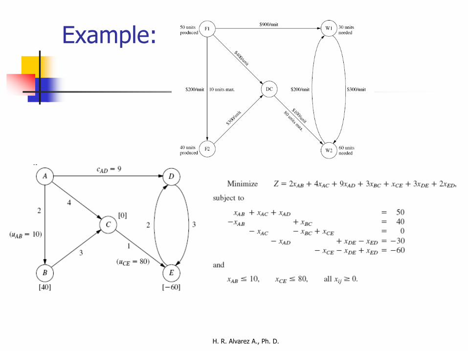
Example:
H. R. Alvarez A., Ph. D.

The Assignment Problem

H. R. Alvarez A., Ph. D.
The Assignment Problem
Suppose that there are n working centers and n possible workers to be assigned, each of one can be assigned to only one of the n centers.
Suppose that there is a cost ci,j of assigning a worker i to a center j.
The objective is to minimize the total assignment cost.

H. R. Alvarez A., Ph. D.
otherwise 0
j center to assigned is i workerif X
n ..., 2, 1, i X
n ..., 2, 1,j X
:.t.s
XCZ.min
j,i
j
ji,
i
j,i
i j
j,ij,i
1
1
1
General formulation

H. R. Alvarez A., Ph. D.
Solution
SIMPLEX Method or binary integer programming
Row Column Method or the Hungarian Method.

H. R. Alvarez A., Ph. D.
The Hungarian Method
The Hungarian method is a combinatorial optimization algorithm which solves the assignment problem in polynomial time.
It was developed and published by Harold Kuhn in 1955.
"Hungarian method" because the algorithm was largely based on the earlier works of two Hungarian mathematicians: Dénes Kőnig and Jenő Egerváry.
The algorithm is known also as Kuhn-Munkres algorithm or Munkres assignment algorithm.

H. R. Alvarez A., Ph. D.
The matrix form of the problem
Given the cost coefficients of an assignment problem such that

H. R. Alvarez A., Ph. D.
Algorithm
1. Row reduction: the lowest of all cij (from j = 1 to n) is taken and is subtracted from each element in that row. This procedure is repeated for all rows.
2. Column reduction: the lowest of all cij (from 1= 1 to m) is taken and is subtracted from each element in that column. This procedure is repeated for all column. The resulting matrix is called the cost reduced matrix.
3. Covering zeroes: Cover all the zeroes in the cost reduced matrix with minimum number of horizontal and vertical lines. If the number of lines is equal to n, the optimal solution was obtained. Otherwise go to the next step.
4. Creating new zeroes: From the covered matrix generated in three, find the smallest element not covered by lines. Subtract this number to all the not covered numbers and add it to the numbers in the intersections of the lines. All the other elements do not change. Go back to step 3.

H. R. Alvarez A., Ph. D.
Example
A restaurant manager wants to serve different customers in different service areas. The manager knows that different client/server combinations may vary service costs due to customer characteristics and servers capabilities. Following is a cost matrix for customers and servers:

H. R. Alvarez A., Ph. D.
Cost for server
Server cost
Customer 1 2 3
1 12.90 11.90 12.10
2 15.30 15.50 14.30
3 11.90 13.90 13.00

H. R. Alvarez A., Ph. D.

H. R. Alvarez A., Ph. D.
Final solution: network representation

One formulation in MPL
H. R. Alvarez A., Ph. D.

Solution
H. R. Alvarez A., Ph. D.
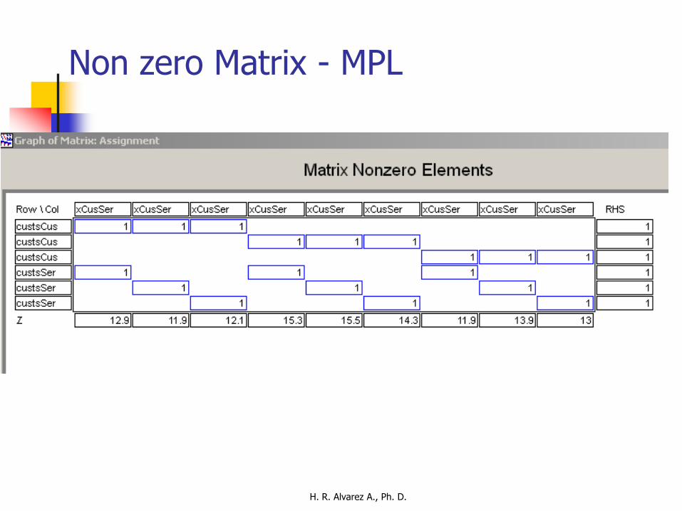
Non zero Matrix - MPL
H. R. Alvarez A., Ph. D.

The transportation problem

H. R. Alvarez A., Ph. D.
The Transportation Problem
Is concerned with distributing any commodity from any group of supply centers, called sources, to any group of receiving centers, called destinations, in such a way as to minimize the total distribution cost.
Each source has a certain supply of units to distribute to the destinations, and each destination has a certain demand for units to be received from the sources.

Assumptions The requirements assumption: means that it needs to be a
balance between the total supply s from all sources and the total demand d at all destinations.
The feasible solutions property: A transportation problem will have feasible solutions if and only if s = d
The cost assumption: The cost of distributing units from any particular source to any particular destination is directly proportional to the number of units distributed.
The model: Any problem (whether involving transportation or not) fits the model for a transportation problem if it can be described completely in terms of a parameter table and it satisfies both the requirements assumption and the cost assumption.
H. R. Alvarez A., Ph. D.

Description A set of m supply points from which a good is
shipped. Supply point i can supply at most si
units.
A set of n demand points to which the good is shipped. Demand point j must receive at least dj units of the shipped good.
Each unit produced at supply point i and shipped to demand point j incurs a variable cost of cij
H. R. Alvarez A., Ph. D.

The parameter table
H. R. Alvarez A., Ph. D.

General formulation
H. R. Alvarez A., Ph. D.
If it is a balanced problem

H. R. Alvarez A., Ph. D.
The general formulation of the balanced problem
A requirement of this problem is that the flow from the sources must be equal to the capacity of the destinations. Otherwise, it is necessary to add either dummy sources or dummy destinations before solving the problem.

The network representation
H. R. Alvarez A., Ph. D.

H. R. Alvarez A., Ph. D.
Solution
Simplex method
Transportation algorithm
Initial Tableau
Initial solution
Optimality test
Redistribution of deliveries

H. R. Alvarez A., Ph. D.
Example
A business delivers products from four areas in the country to four distribution areas including two international . Data shows sources and destination capacities in tons, and the corresponding cost to the different destinations.

H. R. Alvarez A., Ph. D.
Example
Sources Tons
Chiriquí 2,500
Azuero 1,250
Darién 850
Coclé 1,000
Destinations Tons
Panamá 1980
Colón 750
Puerto Balboa 1000
Puerto Cristóbal
1870

H. R. Alvarez A., Ph. D.
Example - Costs
From/To: Panamá Colón Balboa Cristóbal
Chiriquí 50 55 50 55
Azuero 40 48 39 42
Darién 15 25 18 26
Coclé 22 28 25 29

H. R. Alvarez A., Ph. D.
General LP formulation Minimize 50x1,1 + 55x1,2 + … + 25x4,3 + 29x4,4 s. t. : x1,1 + x1,2 + … + x1,4 ≤ 2500 . . . . . . . . . . . . . . . x4,1 + x4,2 + … + x4,4 ≤ 1000 x1,1 + x2,1 + … + x4,1 ≥ 1980 . . . . . . . . . . . . . . . x1,4 + x2,4 + … + x4,4 ≥ 1870
Sources
Destinations

H. R. Alvarez A., Ph. D.
Balanced LP formulation Minimize 50x1,1 + 55x1,2 + … + 25x4,3 + 29x4,4 s. t. : x1,1 + x1,2 + … + x1,4 = 2500 . . . . . . . . . . . . . . . x4,1 + x4,2 + … + x4,4 = 1000 x1,1 + x2,1 + … + x4,1 = 1980 . . . . . . . . . . . . . . . x1,4 + x2,4 + … + x4,4 = 1870
Sources
Destinations

H. R. Alvarez A., Ph. D.
The parameter table:

H. R. Alvarez A., Ph. D.
The network representation

H. R. Alvarez A., Ph. D.
Initial solution– Norwest corner
H. R. Alvarez A., Ph. D.
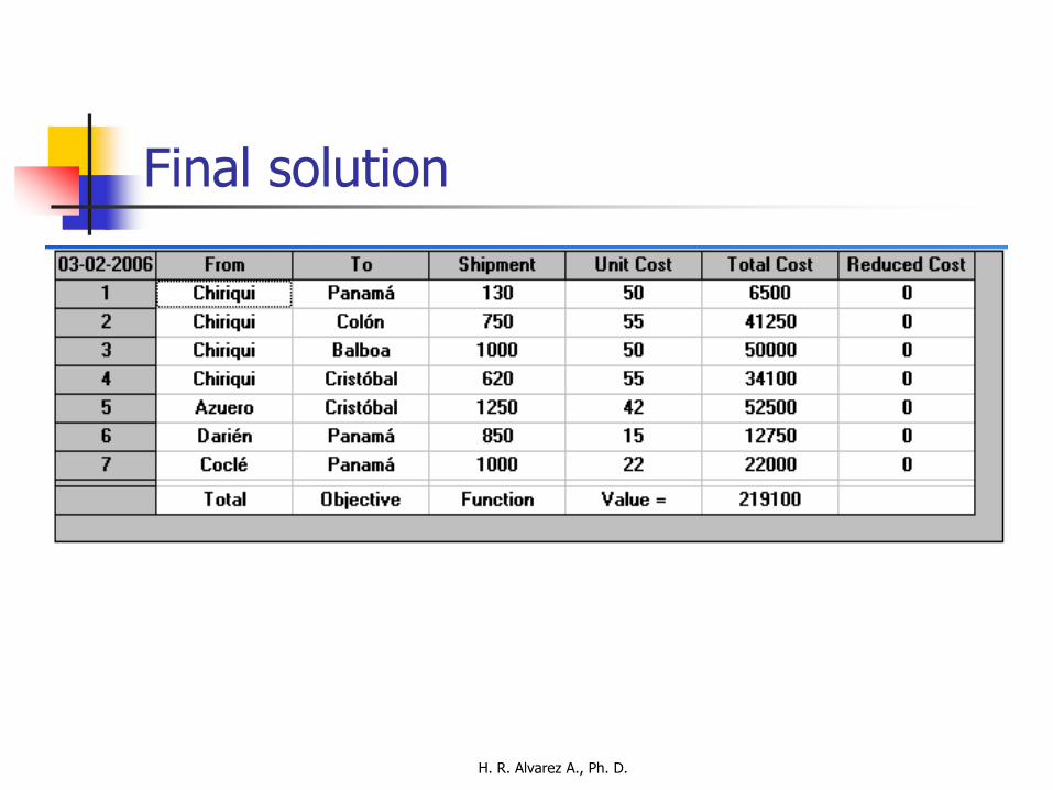
Final solution

H. R. Alvarez A., Ph. D.
Final solution: network representation

One code in MPL
H. R. Alvarez A., Ph. D.

The optimal solution
H. R. Alvarez A., Ph. D.

The optimal solution
H. R. Alvarez A., Ph. D.

The optimal solution
H. R. Alvarez A., Ph. D.

H. R. Alvarez A., Ph. D.
Solver
MPL

The transhipment problem

H. R. Alvarez A., Ph. D.
Description
Normally goods are not directly deliverd to their final destination.
The use intermediate point or distribution centers.
The problem can be described as a minimal flow problem, but with intermediate nodes.

H. R. Alvarez A., Ph. D.

H. R. Alvarez A., Ph. D.
Example
Source Tons
Chiriquí 2,500
Azuero 1,250
Darién 850
Coclé 1,000
Destination Tons
Panamá 1,980
Colón 750
Puerto Balboa 1,000
Puerto Cristóbal
1,870
Distribution Tons
In 3,500
Out 3,500

H. R. Alvarez A., Ph. D.
Costs table
De/A: Panamá Colón Balboa Cristóbal Entrada Salida
Chiriquí 50 55 50 55 20
Azuero 40 48 39 42 18
Darién 15 25 18 26 30
Coclé 22 28 25 29 10
Entrada 5
Salida 15 20 15 20

H. R. Alvarez A., Ph. D.
Chiriquí
Azuero
Darién
Coclé
Entrada Salida
Panamá
Colón
Balboa
Cristóbal

H. R. Alvarez A., Ph. D.
Standard formulation Minimizar 50x1,1 + 55x1,2 + … + 25x4,3 + 29x4,4+ 20x1,5+ 18x2,5+… +10x4,5 + 5x5,6 + 15x6,1 + 20x6,2 + … + 20x6,5
Sujeto a: x1,1 + x1,2 + … + x1,4 + x1, 5 = 2500 . . . . . . . . . . . . x4,1 + x4,2 + … + x4,4 + + x4, 5 = 1000 x5,,6 ≤ 3500 X1,5 + x2,5 + x3,5 + x4,5 = X6,1 + x6,2 + x6,3 + x6,4 = x5,6 x1,1 + x2,1 + … + x4,1 + x6,1 = 1980 . . . . . . . . . . . . x1,4 + x2,4 + … + x4,4 + x6,4 = 1870
Sources
Destination
Flow constraint
Violates the tipical formulation of the transportation problem…

H. R. Alvarez A., Ph. D.
Formulation as a minimal flow problem

H. R. Alvarez A., Ph. D.
Final solution

Formulation and solution in Solver
H. R. Alvarez A., Ph. D.

Comparing solutions
H. R. Alvarez A., Ph. D.

H. R. Alvarez A., Ph. D.
Comparing solutions
Direct Transhipment
Costo 219,100 194,100

H. R. Alvarez A., Ph. D.
Integer linear programming
Only accepts integer solutions
Although the formulation is similar to the LP problem, it has the integrality constraint:
xi {I ≥ 0}

H. R. Alvarez A., Ph. D.
Different types of solutions:
Integer solutions
Binary solutions (0, 1)
Mixed solutions

H. R. Alvarez A., Ph. D.
Solution:
Relaxation: the model does not have the integrality constraint.
The general solution will have all the possible integer solutions.
It is an upper bound in the solution
Rounding up the solution might violate the feasibilty of the problem.

H. R. Alvarez A., Ph. D.
Branch and bound method
Introduced by Land and Doig in 1960
It is a sequential search algorithm
Implicitly enumerates most of the possible solutions of the problem.
It divides the set of possible solution in different subsets.
For every subset, both the upper limits and the feasibility criterium will be used to limit the solution.

H. R. Alvarez A., Ph. D.
General algorithm
1. Find the upper boundary given by the solution of the relaxed model.
2. Define two solution subsets such that d + 1 ≤ xk ≤ d where d is a constant defined by the smallest integer
for the solution for xk
3. For each subset define a new optimal solution: A subset will be fathomed if
- The solution is not feasible - There is a better solution
4. The process stops when an optimal solution with integer variables is found.

H. R. Alvarez A., Ph. D.
Example
Given the following problem
Max.: x = 4x1 + 11x2
s. t.
2x1 – x2 ≤ 4
2x1 + 5x2 ≤ 16
- x1 + 2x2 ≤ 4
x1 y x2 ≥ 0 and integers

H. R. Alvarez A., Ph. D.
x1 ≤ 1 X1 ≥ 2
X2 ≤ 2 X2 ≥ 3
Fathomed

Upper bound solution
H. R. Alvarez A., Ph. D.

Optimal Integer solution in MPL
H. R. Alvarez A., Ph. D.

A slight different formulation
H. R. Alvarez A., Ph. D.