IT15074

Examensarbete 15 hpOctober 2015

Spatial sorting and collective motion in mixed shoals of fish

Markus Eriksson

Institutionen för informationsteknologiDepartment of Information Technology

Teknisk- naturvetenskaplig fakultet UTH-enheten Besöksadress: Ångströmlaboratoriet Lägerhyddsvägen 1 Hus 4, Plan 0 Postadress: Box 536 751 21 Uppsala Telefon: 018 – 471 30 03 Telefax: 018 – 471 30 00 Hemsida: http://www.teknat.uu.se/student

Abstract

Spatial sorting and collective motion in mixed shoalsof fish

Markus Eriksson

Shoaling behaviour arises when fish respond to the movements and positions ofnearby neighbours. The dynamic patterns of shoaling fish has been studied by theMathematical department in Uppsala University. In this project experimental datacollected for groups with two sizes of fish are analysed. An existing model wasmodified to reproduce the dynamic patterns in the fish shoal, this was done bycomparing visual and statistical properties from the simulations with experimentalobservations. By analysing the impact of the parameters in the model it was found outthat introducing limitations in the vision of the smaller fish are essential to be able toreproduce the behaviour of the mixed sized fish shoal. The limitations in the visionare speculated to be a representation of physiological limitations in the coordinationof mechano-sensoric activities and visual information.

ISSN: 1401-5757, UPTEC IT 15 064Examinator: Jarmo RantakokkoÄmnesgranskare: Kristiaan PelckmansHandledare: David J.T. Sumpter och Maksym Romenskyy

Popular Scientific Summary

If you have experienced the fascinating appearance of flocking birds, complex ant net-works or shoaling fish you can get an idea of what the scientists in the field of Collectivebehaviour are working with. Collective behaviour is a relatively new and growing studyfield which goal is to understand and reproduce the complex patterns seen in differentgroups of individuals. By learning the rules that determinate the complex and oftenefficient behaviour we would be able to apply it to human developed systems, such asrobots or to the infrastructure in cities.

In this project the interaction rules that determines the behaviour of a shoal with twosizes of fish are investigated. This was done by the help of experiments and a modeldeveloped at the Mathematical Department in Uppsala University. In the experimentgroups of fifty fish were recorded when they were confined into a circular tank. By modi-fying the existing model and adjusting the model parameters accordingly the result fromthe simulations showed that it was possibly to reproduce the behaviour seen in the ex-periments.

The results from these simulations gave the insight that limitations in the vision field ofthe smaller sized fish in the model were needed to receive the same kind of behaviouras observed in the experiment. These vision limitations could be a representation of theyounger and smaller sized fish not having fully developed central neuron system, whichreduces their ability to coordinate in a shoal.

Acknowledgements

I would like to thank my supervisor Maksym Romenskyy for his greathelp and support.

Thanks also to David J. T. Sumpter for the continuous encouragement.

Contents

1 Introduction 10

2 Material and methods 112.1 Experimental setup and data collection . . . . . . . . . . . . . . . . . . . 112.2 Data processing . . . . . . . . . . . . . . . . . . . . . . . . . . . . . . . . 112.3 Statistics collection . . . . . . . . . . . . . . . . . . . . . . . . . . . . . . 11

3 Model 133.1 Interaction rules . . . . . . . . . . . . . . . . . . . . . . . . . . . . . . . . 133.2 Initial conditions and position updating . . . . . . . . . . . . . . . . . . . 143.3 Boundary condition . . . . . . . . . . . . . . . . . . . . . . . . . . . . . . 143.4 Angular noise . . . . . . . . . . . . . . . . . . . . . . . . . . . . . . . . . 153.5 Modification of the model . . . . . . . . . . . . . . . . . . . . . . . . . . 15

4 Results and discussion 174.1 Experimental results . . . . . . . . . . . . . . . . . . . . . . . . . . . . . 174.2 Model results . . . . . . . . . . . . . . . . . . . . . . . . . . . . . . . . . 194.3 Comparison of positional data . . . . . . . . . . . . . . . . . . . . . . . . 224.4 Conclusions and future work . . . . . . . . . . . . . . . . . . . . . . . . . 23

1 Introduction

When individuals in a group respond to each others movements and positions, a coop-erative complex motion arises. This type of behaviour is called collective motion [1, 2].One of the main goals in the research of collective motion is to understand and makeclassification of the interaction rules leading to the flocking behaviour that can be ob-served in groups of different species [3, 4]. The fish is an animals that can be modelledby implementing a set of simple behavioral rules and when each individual follows thoserules complex patterns emerges [5, 6]. The study of the shoaling dynamics are of spe-cial interest since fish is a convenient animal to use in experiments and modelling. Bylearning more about the shoaling dynamics it would be possible to get a better insight inthe collective motion of other systems of individuals. The research group lead by D.J.T.Sumpter at the Mathematics Department in Uppsala University have been working onthe study of collective animal behaviour with a focus on on the shoaling behaviour offish. In an experiment different amounts and sizes of the fish species Pacific blue eyeswas confined in a shallow circular tank and filmed from above. By analysing the videosthey found that the shoaling behaviour of groups with only big sized fish, groups withonly small sized fish and groups with mixed sized fish behave differently from each other.The group with only big sized fish tend to move cohesively, with high speed close to thewall. The group with only small sized fish tend to move with less cohesiveness, with lowspeed and distributed all over the tank. For the group of mixed sized fish the big sizedfish had the same behaviour as in the case with only big sized fish while the small sizedfish changed their behaviour to move with more cohesiveness and going in the same an-gular direction as the big sized fish but closer to the center of the tank. The observationsindicate that the small sized fish tries to adapt to the motion of the big sized fish. Byimplementing a computer based model the research team could reproduced the behaviourof the groups with only big sized fish and small sized fish. In this project it was my taskto reproduce the collective motion of the group with mixed sized fish, by modifying themodel and tuning the parameters in a qualitative manner so the same behaviour seen inthe experiments could be received and make quantitative interpretations of the results.

10

2 Material and methods

2.1 Experimental setup and data collection

The fish species used in the experiment was Pacific blue eyes, Pseudomugil signifer.Groups of 50 fish were used with two different sizes of the fish, small sized fish with thebody length 7.5 mm and big sized fish with the body length 20 mm. The fractions ofbig sized fish in the mixed sized groups were 0.2, 0.3 and 0.4, i.e. the fraction is 0.2when 20% of fish in a group are big sized fish. The fish were confined into a large (760mm in diameter) shallow circular arena and recorded from above. The camera used wasa Logitech C615. Each video had the duration of 15 to 20 minutes, recorded with theframe rate of 15 frames per second. In total, ten experimental trials were filmed and thevideos were compressed to AVI-format. The tracking software DIDSON [7] was used toconvert the position of the fish in the videos into MAT-file format with the X-coordinate,Y-coordinate, ID-number and with the corresponding time step. The pixel-to-mm ratiowas 1.4755. The classification of the fish size was done by manually picking out whichID-numbers corresponded to big sized fish and small sized fish.

2.2 Data processing

The videos were examined visually to analyse specific spatial patterns of the fish so thatthe model parameters could be tuned and the statistical collections from the experimentcould be validated. MATLAB was used to analyse the experimental data by visualizingthe tracking data of the fish and calculating the statistical properties of the shoals. Thetracking data contained approximately 30% errors that were caused by a too coarseresolution in the recording of the videos which lead to inconsistencies when the fish wereswimming close to each other, some of the time steps were not tracked for some fish andthe ID-numbering of the fish changed owner from time to time, therefore the data hadto be processed to make the tracking data consistent. The first approach to solve theinconsistencies were to use parts of trajectories with consistent identities. The result wasrealistic plots but with too few time frames to be used to do quantitative interpretations.Then the approach was changed to implementing a filter algorithm that tracked the fishuntil they did an unrealistically large change in position, the result was that the majorityof the time frames contained small sized fish since the big sized fish had higher probabilityto make a large change in position and the simulation was to no use. The final approachwas to manually do the classification for each time frame for the fish size for one of thevideos, this resulted in consistent plots with large enough number of frames to be usedto do statistical analysis of the simulations.

2.3 Statistics collection

From the tracking data the velocities of each fish can be calculated based on two subse-quent positions. The positions and velocities could be used to calculate the radial densitydistribution g(r), the polar order parameter ϕ(r) and the angular order parameter L(r).The statistics were calculated by dividing the tank into ten circular shells, with the shellradius 38, 76, ..., 380 mm, where each fish could be positioned in one of shells at eachtime step.The normalized density g(r) quantifies the distribution of fish across the tank in radialdirection and was calculated as in [8]

11

Figure 1: Figure demonstrating three circular shells. ri is the position vector from thecenter of the tank to the center of the fish i and r is the half-shell-width.

g(r) =1

πr21

N(r)

�N(r)�

i=1

δ(r − |ri|)�

(1)

where δ is the Dirac delta function, |ri| is the euclidean distance from the center of thetank to the fish i, r is the half-shell-width, < . > stands for the ensemble average andN(r)is the amount of fish inside the circular shell given by r. The angular order parameter isa scale free measurement of the sum of the angular momenta of the fish, it is the degreeof rotation of the group about the centre of the tank and takes a value in the interval[0, 1]. The angular order parameter L(r) is calculated as in [6]

L(r) =

������

N(r)�

i=1

ri × vi

|ri||vi|

������(2)

and is calculated for every shell. vi is the velocity and ri is the position of the fish. Thepolar order parameter ϕ(r) is a measurement of how strong the alignment within a groupis, it is calculated as in [6]

ϕ(r) =

�N(r)i=1 vi�N(r)j=1 |vj|

(3)

and is calculated for every shell. The nearest-neighbour distance was calculated by

NNi = mini �=j

rij (4)

where rij is the euclidean distance between fish i and j.

12

3 Model

3.1 Interaction rules

In the model the fish are moving with a constant propulsion speed and the direction ofmotion is calculated by obeying interaction rules on the surrounding neighbours, withsome random perturbation added.

Figure 2: Zones of interactions. Each zone starts from the center of the fish i. vi is thevelocity of fish i, Rr is the radius of the repulsion zone, β is the blind angle and Ra is theradius of the alignment zone.

The interaction rules are that for each time step

• The fish repulse from their neighbours that are positioned inside their repulsionzone that has the radius Rr, to avoid collision.

• If the fish does not have any neighbours inside their repulsion zone but there areneighbours inside the zone of alignment, that has the radius Ra, it aligns with theaverage direction of motion of the fish inside the alignment zone.

• If some neighbours of the fish are in the area of the blind angle, defined by theangle β, the focal fish will not align with those neighbours.

• If there are no fish inside the zone of repulsion or in the alignment zone the fishwill continue their movement unaffected by other fish.

The velocity was calculated as in [8]

vi(t) = v0ui(t)R1(ξi(t))R2(ωi(t)) (5)

where

ui(t) = −nr�

j �=i

rij(t)/

�����

nr�

j �=i

rij(t)

����� (6)

or

ui(t) =na�

j=1

vj(t)/

�����

na�

j=1

vj(t)

�����. (7)

13

Equation (6) is used for repulsion interactions and equation (7) is used for alignmentinteractions [6]. u is the unit vector of the direction of motion. v0 is the speed of thefish, which is a fixed value in this model. rij is the euclidean distance between the fish iand the fish j. R1 is a rotation matrix which is used to calculate the angular noise whereξi(t) is a random number in the interval −π to π used to rotate fish i. R2 is a rotationmatrix which is used to calculate the influence the wall has on the fish, where ωi(t) isthe turning rate the fish i will change the direction of motion with. The definition of therotation matrix is

R(θ) =

�cos(θ) −sin(θ)sin(θ) cos(θ)

�(8)

where θ is the turning angle.

3.2 Initial conditions and position updating

The time integration and the statistical collection in the model was implemented by usingthe program language FORTRAN and compiled with a GFortran compiler. MATLAB wasused to visualize the movement and plotting the statistical properties. The simulationswere carried out in a circular shaped cell with the radius 380 pixels and integrated for50 000 time steps at each run. The fish were initially positioned with a random uniformdistribution in the cell with random uniformly distributed directions. At each time steppositions of all fish were streamed along to their new direction by using the equation

ri(t+ 1) = ri(t) +∆tvi(t) (9)

where the time unit ∆t was set to one and the velocity was calculated by equation (5).

Table 1: Parameters used in the model.Parameter Value Descriptionηbig 0.1 Noise parameter for the big sized fish.ηsmall 0.0 to 1.0 Noise parameter for the small sized fish.Ra,big 96 Alignemnt zone radius for the big sized fish.Ra,small 30.0, 51.9 or 92.3 Alignment zone radius for the small sized fish.v0,big 10 Speed of the big sized fish.v0,small 1 to 9 Speed of the small sized fish.βbig 0 rad Blind angle for the big sized fish.βsmall 0 to 2π rad Blind angle for the small sized fish.Rr 10 Repulsion zone radius.fraction 0.0 to 1.0 Fraction of big sized fish.

In Table 1 the parameters used in the model are stated, some of the parameters are tunedwithin a range specified in the table for different simulations to get motion patterns similarto those observed in the experiment. The repulsion zone radius and alignment zone radiusparameter values were estimated experimentally.

3.3 Boundary condition

The boundary condition is modeled as a repulsion from the wall and is calculated as in[11]

14

ωi(t) = v0αi(t)

di(t)(10)

where αi is the angle between the direction of motion of the fish i and the normal to thepoint of impact on the wall and di is the euclidean distance from fish i to the point ofimpact on the wall. ωi is the turning rate with which the fish i will change direction ofmotion due to the wall repulsion when time integrating by equation (5). These parameterscan be seen in figure 3.

Figure 3: Parameters used to calculate the wall influence on the fish i in the model

3.4 Angular noise

To get realistic fish movement behavior the angular noise has to influence the fish when thedirection of motion is integrated. If noise is to weak the fish will move with a unrealisticrobotic behaviour while under influence of strong noise the fish will move with a randomin-cohesive behaviour. The angular noise is calculated by using the Gaussian distributedprobability density function

P (ξi(t)) = e−ξ2i (t)/2η2/�2ξi(t)η (11)

where η is the noise parameter that is a value chosen between zero and one to tune howbig the influence of angular noise is when integrating the direction of motion in equation5. For each simulation a different initial seed was used in the random number generatorfunction calls to avoid repeated motion patterns.

3.5 Modification of the model

To be able to use the existing model modifications had to be made to support mixedsized group where fish had different properties. The following modifications were madeto the existing model

• Introduced a fraction variable for different ID-numbers of the fish to correspond toa big sized fish or small sized fish, which made it possible to distinguish the differentproperties.

• Implemented the support for the big sized fish and the small sized fish to move withdifferent constant speeds.

• Implemented the support for the big sized fish and the small sized fish to havedifferent alignment zone radius.

15

• Implemented the support for the big sized fish and the small sized fish to interactwith different blind angles.

• Implemented an independent control over the noise parameter η for small and largefish.

• Implemented the support for the statistical collection to do separate calculationsfor the big sized fish and the small sized fish.

• Introduced shell statistics where statical collection could be done to see radial dis-tance dependencies, with separate calculations for the big sized fish and the smallsized fish.

The parameters in the modified model had to be tuned to achieve similarity in statisticalbehaviour. This was done by iteratively changing one parameter at a time and comparingthe visualization of the result and the statistical collection from the simulations with thevideos and the statistical collection from the experiment.

16

4 Results and discussion

4.1 Experimental results

The results from the experiment are calculations made on the tracking data from threeof the videos. One video of the mixed sized group where the fraction of big sized fishwas 0.4, one video of the group containing only big sized fish and one video of the groupcontaining only small sized fish.

(a) Group of mixed sized fish (b) Group of big sized fish (c) Group of small sized fish

Figure 4: Snapshots of the observation of the three different videos recorded in theexperiment, with an overlay of the tracked data visualized by blue dots for big sized fishand red dots for small sized fish.

In figure 4 the typical movement behaviour of the three different groups are seen. In thegroup of mixed sized fish the big sized fish are moving cohesively positioned close to thewall of the tank while the small sized fish are moving with some cohesiveness positionedclose to the center of the tank. In the group with only big sized fish the group is movingcohesively close to the wall of the tank. In the group with only small sized fish the groupis moving with little cohesiveness and the fish are positioned all over the tank.

(a) (b) (c)

Figure 5: Statistics from the experiment on the mixed sized group: (a) Normalized densitydistribution, (b) polar order parameter and (c) angular order parameter as a functionsof radial distance.

In figure 5 the statistics from the experiment on the mixed sized group is seen. Thenormalized density distribution shows that the big sized fish is distributed close to thewall of the tank, with a density distribution peak at the radial distance 670 mm, and

17

that the small sized fish are distributed close to the center of the tank, with a densitydistribution peak at the center of the tank. The polar order parameter shows that bigsized fish has increasing polar order as the radial distance is increasing, with a polar orderpeak at the radial distance 680 mm, and that the small sized fish has decreasing polarorder as the radial distance is increasing, with a polar order peak at the radial distance340 mm. The angular order parameter shows that big sized fish has increasing angularorder as the radial distance is increasing, with a angular order peak at the radial distance680 mm, and that the small sized fish has a peak at the radial distance 420 mm.

(a) (b) (c)

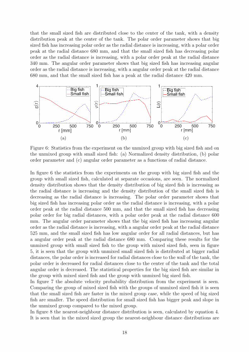
Figure 6: Statistics from the experiment on the unmixed group with big sized fish and onthe unmixed group with small sized fish: (a) Normalized density distribution, (b) polarorder parameter and (c) angular order parameter as a functions of radial distance.

In figure 6 the statistics from the experiments on the group with big sized fish and thegroup with small sized fish, calculated at separate occasions, are seen. The normalizeddensity distribution shows that the density distribution of big sized fish is increasing asthe radial distance is increasing and the density distribution of the small sized fish isdecreasing as the radial distance is increasing. The polar order parameter shows thatbig sized fish has increasing polar order as the radial distance is increasing, with a polarorder peak at the radial distance 500 mm, and that the small sized fish has decreasingpolar order for big radial distances, with a polar order peak at the radial distance 600mm. The angular order parameter shows that the big sized fish has increasing angularorder as the radial distance is increasing, with a angular order peak at the radial distance525 mm, and the small sized fish has low angular order for all radial distances, but hasa angular order peak at the radial distance 680 mm. Comparing these results for theunmixed group with small sized fish to the group with mixed sized fish, seen in figure5, it is seen that the group with unmixed small sized fish is distributed at bigger radialdistances, the polar order is increased for radial distances close to the wall of the tank, thepolar order is decreased for radial distances close to the center of the tank and the totalangular order is decreased. The statistical properties for the big sized fish are similar inthe group with mixed sized fish and the group with unmixed big sized fish.In figure 7 the absolute velocity probability distribution from the experiment is seen.Comparing the group of mixed sized fish with the groups of unmixed sized fish it is seenthat the small sized fish are faster in the mixed group case, while the speed of big sizedfish are smaller. The speed distribution for small sized fish has bigger peak and slope inthe unmixed group compared to the mixed group.In figure 8 the nearest-neighbour distance distribution is seen, calculated by equation 4.It is seen that in the mixed sized group the nearest-neighbour distance distributions are

18

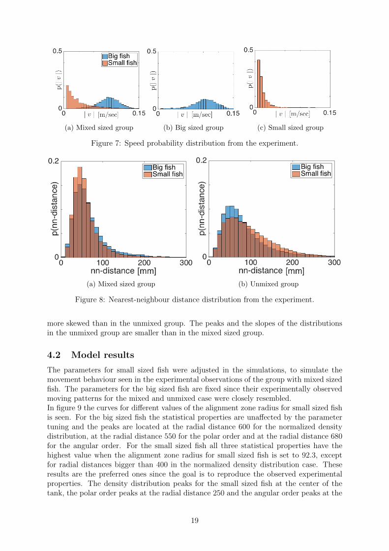
(a) Mixed sized group (b) Big sized group (c) Small sized group

Figure 7: Speed probability distribution from the experiment.

(a) Mixed sized group (b) Unmixed group

Figure 8: Nearest-neighbour distance distribution from the experiment.

more skewed than in the unmixed group. The peaks and the slopes of the distributionsin the unmixed group are smaller than in the mixed sized group.

4.2 Model results

The parameters for small sized fish were adjusted in the simulations, to simulate themovement behaviour seen in the experimental observations of the group with mixed sizedfish. The parameters for the big sized fish are fixed since their experimentally observedmoving patterns for the mixed and unmixed case were closely resembled.In figure 9 the curves for different values of the alignment zone radius for small sized fishis seen. For the big sized fish the statistical properties are unaffected by the parametertuning and the peaks are located at the radial distance 600 for the normalized densitydistribution, at the radial distance 550 for the polar order and at the radial distance 680for the angular order. For the small sized fish all three statistical properties have thehighest value when the alignment zone radius for small sized fish is set to 92.3, exceptfor radial distances bigger than 400 in the normalized density distribution case. Theseresults are the preferred ones since the goal is to reproduce the observed experimentalproperties. The density distribution peaks for the small sized fish at the center of thetank, the polar order peaks at the radial distance 250 and the angular order peaks at the

19

(a) (b) (c)

Figure 9: Tuning of the small sized fish alignment zone radius parameter in the model:(a) Normalized density distribution, (b) polar order parameter and (c) angular orderparameter as a functions of radial distance. The continuous lines are small sized fish andthe dashed lines are big sized fish. With the parameters set to ηbig = 0.1, ηsmall = 0.2,Ra,big = 92.3, v0,big = 10, v0,small = 4, βbig = 0 rad βsmall = 0.93 rad, Rr = 10 andfraction = 0.4.

radial distance 340.

(a) (b) (c)

Figure 10: Tuning of the small sized fish blind angle [rad] parameter in the model:(a) Normalized density distribution, (b) polar order parameter and (c) angular orderparameter as a functions of radial distance. The continuous lines are small sized fish andthe dashed lines are big sized fish. With the parameters set to ηbig = 0.1, ηsmall = 0.2,Ra,big = 92.3, Ra,small = 92.3, v0,big = 10, v0,small = 4, βbig = 0 rad, Rr = 10 andfraction = 0.4.

In figure 10 the curves for different values of the blind angle for the small sized fish arepresented. It is seen that setting the blind angle for small sized fish to 0 rad gives statis-tics that are similar to the statistics of the big sized fish. Setting the blind angle for thesmall sized fish to 0.93 rad gives the density distribution with the small sized fish locatedclosest to the center of the tank, it also gives the lowest value of the polar order andthe angular order at radial distances close to the wall. For the big sized fish the statisti-cal properties are unchanged and the peaks are located at the same positions as in figure 9.

In figure 11 the curves for different values of the noise parameter for small sized fish isseen. It is seen that setting the noise parameter for small sized fish to 0.1 or 0.05 thehighest values on the statistical properties close to the center of the tank for the small

20

(a) (b) (c)

Figure 11: Tuning of the small sized fish angular noise parameter in the model: (a) Nor-malized density distribution, (b) polar order parameter and (c) angular order parameteras a functions of radial distance. The continuous lines are small fish and the dashedlines are big fish. With the parameters set to ηbig = 0.1, Ra,big = 92.3, Ra,small = 92.3,v0,big = 10, v0,small = 4, βbig = 0 rad βsmall = 0.93 rad, Rr = 10 and fraction = 0.4

sized fish are received, for those values the density distribution is peaking at the radialdistance 180, the polar order is peaking at the radial distance 260 and the angular orderis peaking at the radial distance 350. For the big sized fish the statistical properties areunchanged and the peaks are located at the same positions as in figure 9.

(a) (b) (c)

Figure 12: Statistic collection of the simulations on the unmixed groups of big sized fishand small sized fish: (a) Normalized density distribution, (b) polar order parameter and(c) angular order parameter as a functions of radial distance. With the parameters setto ηbig = 0.1, ηsmall = 0.2, Ra,big = 92.3, Ra,small = 92.3, v0,big = 10, v0,small = 4, βbig = 0rad βsmall = 0.93 rad, Rr = 10 and fraction = 0.4

In figure 12 the statistics from the simulations of the case with unmixed groups of big sizedfish and a small sized fish are seen. The parameters were set to ηbig = 0.1, ηsmall = 0.2,Ra,big = 92.3, Ra,small = 92.3, v0,big = 10, v0,small = 4, βbig = 0 rad βsmall = 0.93 rad,Rr = 10 and fraction = 0.4. Those parameters were chosen to reproduce the spatialpatterns and statistical properties observed in the experiment with groups of mixed sizedfish. It is seen that the small sized fish are evenly distributed in the tank while the bigsized fish are distributed close to the wall of the tank with a density distribution peakat the radial distance 600. The small sized fish has a polar order parameter peaks atthe radial distance 300 and the big sized fish has a polar order parameter peaks at theradial distance 500. The small sized fish angular order parameter is increasing as the

21

radial distance is increasing and for the big sized fish the angular order parameter peaksat the radial distance 510. Comparing the simulations of the group with mixed sized fishand the unmixed groups it is seen that the movement behaviour of the big sized fish aresimilar in both cases but the movement behaviour of the small sized fish are changed,one of the biggest changes in the behaviour for the small sized fish are that they aredistributed closer to the center of the tank in the group with mixed sized fish.

(a) Mixed sized group (b) Unmixed groups

Figure 13: Nearest-neighbour distance distribution from the model. With the parametersset to ηbig = 0.1, ηsmall = 0.2, Ra,big = 92.3, Ra,small = 92.3, v0,big = 10, v0,small = 4,βbig = 0 rad, βsmall = 0.93 rad, Rr = 10 and fraction = 0.4.

In figure 13 the nearest-neighbour distance distribution is seen, calculated by equation 4.It is seen that in the mixed sized group the nearest-neighbour distance distribution for thesmall sized fish is more skewed than in the unmixed group. The peak of the distributionfor the small sized fish in the mixed sized group is bigger than in the unmixed group.

4.3 Comparison of positional data

Some of the comparison made between the visualization of the simulations and the videosfrom the experiment with tracking data is in this section presented trough snapshots.In figure 14 snapshots from the experiment and the model for the group with mixed sizedfish are seen. In the figure the similarities in the collective motion is observed, the bigsized fish tend to move cohesively distributed close to the wall of the tank while the smallsized fish tend to move cohesively distributed close to the center of the tank and followingthe angular movement of the big sized fish.In figure 15 snapshots from the experiment and the model for the group with big sizedfish is seen. In the figure the similarities in the collective motion is observed, the bigsized fish tend to move cohesively positioned close to the wall.In figure 16 the snapshots from the experiment and the model for the groups with smallsized fish is seen. In the figure the similarities in the collective motion is seen, the smallsized fish tend to move with little cohesiveness and distributed all over the tank.

22

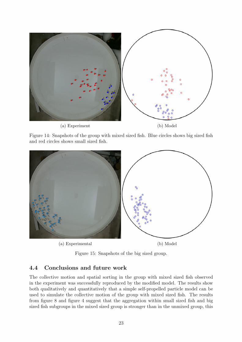
(a) Experiment (b) Model

Figure 14: Snapshots of the group with mixed sized fish. Blue circles shows big sized fishand red circles shows small sized fish.

(a) Experimental (b) Model

Figure 15: Snapshots of the big sized group.

4.4 Conclusions and future work

The collective motion and spatial sorting in the group with mixed sized fish observedin the experiment was successfully reproduced by the modified model. The results showboth qualitatively and quantitatively that a simple self-propelled particle model can beused to simulate the collective motion of the group with mixed sized fish. The resultsfrom figure 8 and figure 4 suggest that the aggregation within small sized fish and bigsized fish subgroups in the mixed sized group is stronger than in the unmixed group, this

23

(a) Experimental (b) Model

Figure 16: Snapshots of the small sized group.

behaviour has been reproduced in the simulations seen in figure 13. The parameters thatmake the dynamics in the model similar to experimental observations are the alignmentzone of the small sized fish, the noise parameter for the small sized fish and the blindangle for the small sized fish. Introducing a blind angle is essential in order to reproducethe behaviour of small sized fish within a mixed group. From the tested values on theblind angle for small sized fish the value 0.93 rad was the optimal, which is seen in fig-ure 10. The biological properties of fish bodies give them limited vision directly behindthem. In mathematical models, these limitations are traditionally introduced in a formof blind angle [9]. In a broader sense, it can be speculated that the blind angle can bealso used as a representation of the physiological limitation on a level of coordination ofmechano-sensoric activities and visual information [10]. The younger small sized fish maynot yet fully developed their neuron and muscular system and therefore cannot respondfast to changing environment or support large swimming speeds. From a physical pointof view the blind angle allows to tune a degree of anisotropy of interactions between theindividuals in the system. If the blind angle is equal to zero the interactions are fullyisotropic which corresponds to fish with more developed central nervous systems. If theblind angle is increased more limitations are imposed which corresponds to fish with lessdeveloped central nervous systems. Lower level of mechanical activity can be simulatedby assigning the fish lower propulsion speeds.

Improvements that could be made to give more reliable results is to use a camera and/ortracking software that tracks the fish with more consistency, this would make it possibleto more effectively use tracking data from the videos. The tuning of the parameters couldbe done more precise if an automatic parameter fitting algorithm was implemented witha optimized time-integrator.

24

References

[1] Vicsek T., Zafeiris A., 2012. Collective motion, Physics Reports 517(2012)71-140.

[2] Sumpter D.J.T., Richard P.M and Perna A., The modeling cycle for collective animalbehaviour, Interface Focus (2012) 2, 764-773. August 2012.

[3] Vicsek T., Czirok, A., Ben-Jacob, E., Cohen I., Shochet O., 1995, Novel Type of PhaseTransition in a System of Self-Driven Particles, Physical Review Letters 75, 1226.

[4] Sumpter D.J.T., 2010, Collective Animal Behaviour, Princeton University Press.

[5] Herbert-Read J.E., Perna A., Mann R.P., Schaerf T.M., Sumpter D.J.T. and WardA.J.W. Inferring the rules of interaction of shoaling fish, PNAS 18726-18731, Novem-ber 15 2011, vol. 108, no. 46.

[6] Couzin D.I., Krause J., James R., Ruxton G.D., Franks N.R., 2002. Collective Memoryand Spatial Sorting in Animal Groups, J. theor. Biol. (2002) 218, 1-11.

[7] Handegard N.O. and Williams K., ICES Journal of Marine Science, Journal du Con-seil 65, 636 (2008).

[8] Romenskyy M. and Lobaskin V., Statistical properties of swarms of self-propelledparticles with repulsion across the order-disorder transition. Eur. Phys. J. B (2013)86: 91.

[9] Domenici P. and Blake R., The Journal of Experimental Biology 200, 11651178 (1997).

[10] Romenskyy M.,Lobaskin V. and Ihle T., Tricitical points in a Vicsek model of self-propelled particles with bounded confidence, Physical Review E90, 063315 (2014).

[11] Romenskyy M., Herbert-Read J.E., Ward A.J.W. and Sumpter D.J.T., Analysingand Modelling the Statistical Properties of Schooling Fish, 2015, in preparation.

[12] Strombom D., Siljestam M., Park .J and Sumpter D.J.T., The shape and dynamicsof local attraction, Department of Mathematics, Uppsala University, 2013.

[13] Masuda R. and Tsukamoto K., The ontogeny of schooling behavior in the stripedjack, Journal of Fish Biollogy (1998) 52, 483-493.

25