Environmental ManagementDOI 10.1007/s00267-016-0741-z

Spatial patterns of air pollutants and social groups: a distributiveenvironmental justice study in the phoenix metropolitan regionof USA

Ronald Pope1 ● Jianguo Wu1,2 ● Christopher Boone2

Received: 29 May 2015 / Accepted: 15 July 2016© Springer Science+Business Media New York 2016

Abstract Quantifying spatial distribution patterns of airpollutants is imperative to understand environmental justiceissues. Here we present a landscape-based hierarchicalapproach in which air pollution variables are regressedagainst population demographics on multiple spatio-temporal scales. Using this approach, we investigated thepotential problem of distributive environmental justice inthe Phoenix metropolitan region, focusing on ambientozone and particulate matter. Pollution surfaces (maps) areevaluated against the demographics of class, age, race(African American, Native American), and ethnicity (His-panic). A hierarchical multiple regression method is used todetect distributive environmental justice relationships. Ourresults show that significant relationships exist between thedependent and independent variables, signifying possibleenvironmental inequity. Although changing spatiotemporalscales only altered the overall direction of these relation-ships in a few instances, it did cause the relationship tobecome nonsignificant in many cases. Several consistentpatterns emerged: people aged 17 and under were sig-nificant predictors for ambient ozone and particulate matter,but people 65 and older were only predictors for ambientparticulate matter. African Americans were strong

predictors for ambient particulate matter, while NativeAmericans were strong predictors for ambient ozone. His-panics had a strong negative correlation with ambientozone, but a less consistent positive relationship withambient particulate matter. Given the legacy conditionsendured by minority racial and ethnic groups, and therelative lack of mobility of all the groups, our findingssuggest the existence of environmental inequities in thePhoenix metropolitan region. The methodology developedin this study is generalizable with other pollutants to pro-vide a multi-scaled perspective of environmental justiceissues.

Keywords Environmental justice ● Spatiotemporal scale ●

Ozone ● PM10● Scale effects ● Phoenix metropolitan region

Introduction

Environmental justice can be a field of study for research-ers, a public policy goal for government regulators, or asocial movement by stakeholders who are concerned aboutthe environment in which they live (Brulle and Pellow2006). The environmental justice movement is rooted in thecivil rights era and many of the historic early studiesdetailed the link between race and the inequitable siting oftoxic industries (United Church of Christ (UCC) 1987;Bullard 1990). Based on evidence of inequitable conditionsdemonstrated in these and other important studies, a Pre-sidential Executive Order (12898) mandated that federalagencies consider environmental justice issues in theirpolicies and actions (Cutter and Solecki 1996).

Environmental justice principally addresses two types ofjustice: procedural and distributive. Procedural justice is

* Ronald Poperpope@asu.edu

1 School of Life Sciences, Arizona State University, Tempe, AZ85287, USA

2 School of Sustainability, Arizona State University, Tempe, AZ85287, USA

Electronic supplementary material The online version of this article(doi:10.1007/s00267-016-0741-z) contains supplementary material,which is available to authorized users.

often defined as fair application of environmental laws andpolicies for all groups of people. Distributive justice is thefair or equitable distribution of environmental benefits andburden across all social groups, often examined in spatialterms by neighborhoods (Rechtschaffen 2003). Studies indistributive environmental justice examine relationshipsbetween social demographics, such as race and class, andpatterns of environmental conditions, such as proximity tosources of pollution, the quality of ambient air or waterresources, or even blighted and polluted neighborhoods(Boone et al. 2014). When these inequitable conditions arebrought to light, policy makers can use that knowledge torectify the situation or citizens can use the information toargue for improved environmental conditions.

This paper describes a novel methodology for studyingdistributive environmental justice by comparing demo-graphics at the census block group level to multiple spa-tiotemporal scales of monitored pollution so as to determinethe multi-scalar extent of environmental inequity. Themethodology developed here is based on methods fromlandscape ecology and utilizes geographical informationsystem (GIS) and network-based approaches to create pol-lution models. Landscape ecology, a discipline devoted tounderstand the spatial relationships between scales, pat-terns, and processes, offers useful methods and insight intothe creation of these pollution models. The primary aim ofthis methodology is to explore and highlight the differencesin results between multiple spatiotemporal scales in theanalysis. The methodology described here is generalizableto other studies using pollution data that is multiscalar inspace and time.

In this paper, we detail a case study of distributiveenvironmental justice in Phoenix, Arizona using this multi-scalar methodology. It focuses on ambient air quality col-lected from government air monitoring networks andexamines how distinct socioeconomic groups are exposedto ground-level ozone (O3) and particulate matter less than10 µ in size (PM10), the two criteria pollutants of mostconcern in this area. Acknowledging that environmentaljustice can be more complicated than just the distribution ofpollutants, we discuss some of the legacy conditionsexperienced by minority populations in the Phoenix area;but we focus mainly on the utilization of landscape ecolo-gical methods to create multi-scale pollution models, basedupon actual monitored pollution concentrations, to test forpossible distributive justice issues based on neighborhooddemographics.

Spatiotemporal Scale in the Environmental JusticeLiterature

A number of environmental justice studies consider oraddress scale (i.e., the areal unit of analysis) or scope (i.e.,

the geographic bounds of the study) issues using variousmethods. For example, Cutter et al. (1996) conducted ajustice study in South Carolina to see how hazardous wasteand toxics releasing facilities affect low-income minoritygroups at three different spatial scales: counties, censustracks, and census block groups. Associations were found atthe county level, but not at finer scales. Huby et al.’s (2009)justice study in England stresses the need for multi-scaleanalysis, and notes that coarser scales can mask inequalitiesdue to aggregation. Baden et al.’s (2007) review of existingempirical justice literature shows that studies span a rangeof scales, some employ multi-scale methods, but few usemultiple units of analysis. Variation was observed acrossthe methods, but the authors note that smaller scales tend toexhibit more statistically insignificant findings, concludingthat scale and scope can strongly influence analysis andresults (Baden et al. 2007).

Choosing the scale of analysis is important as differentscales can produce different results and using one scale tomake inferences about another scale can lead to falsedeductions—phenomena known as the modifiable areal unitproblem (MAUP) and the ecological fallacy, subjects oftenaddressed in landscape ecology (Wu 2007). The MAUPpresents two interrelated problems with spatial data analy-sis: the scaling problem and the zoning problem (Wu 2007;Jelinski and Wu 1996; Openshaw 1984). The scaling pro-blem is due to the aggregation of smaller units into fewerand larger geographical units increasing correlation, butreducing variation; while the zoning problem results fromthe drawing of spatial boundaries that can create falsecategories of data and is related to gerrymandering.Researchers have tried different methods of analysis toavoid the issues of the MAUP, such as using the hedonicprice method (Noonan et al. 2009) or dasymetric mapping(Giordano and Cheever 2010; Boone 2008), with varyingfindings. Presenting results from multiple scales can also beeffective against the MAUP, as an inequity observed at anyscale can arguably be considered evidence of an injustice(Baden et al. 2007).

The temporal scale of analysis is equally important infinding environmental inequity, especially when usingambient air pollution as the environmental medium.Although temporal scale of the analysis or data is oftenmentioned (Jerrett et al. 2001), there is a deficit of envir-onmental justice literature addressing multiple-scale tem-poral analysis methods (Noonan 2008). The methodologyand case study described in this paper will address thisdeficit by exploring spatiotemporal patterns at multiplescales.

There have also been a number of previously conductedenvironmental justice studies in the Phoenix metropolitanarea using different techniques and scales. These techniquestypically find environmental inequities, depending on the

Environmental Management

observed scale, the method used, and the medium investi-gated. For instance, the Bolin et al. (2000) study investi-gated point sources of toxic emissions to determineenvironmental equity problems with the location, volume,and toxicity of emissions. Their study found that minoritypopulations in South Phoenix faced injustices when com-pared with the location of industries or volume of emis-sions, but not toxicity of emissions as many high-techindustries, implicated with emissions of greater toxicity, arelocated in more affluent areas of Phoenix away from thehigher density locations of minority populations. A similarspatial analysis by Bolin et al. (2002) found equity issuesbetween race and class and point sources of hazardouswaste industries and large quantity generators. Grineskiet al. (2007) quantified air pollution by laying a grid over anambient pollution surface of carbon monoxide, nitrousoxides (NOx), and O3, modeled in a 1 h time resolution, andanalyzed the pollutant levels to the race and class compo-sition of associated neighborhoods. They found equityissues for Latinos and Native Americans, but not AfricanAmericans. Grineski (2007) used the same pollution model,along with the Toxics Release Inventory and a proxy forindoor pollution hazards, to look for equity issues withasthma cases. They found that African Americans experi-enced injustices, but Latinos were not significant predictorsfor rates of asthma hospitalization. Native Americans werenot included in that study.

These Phoenix-based studies employed a number ofdifferent methods to find justice issues over different spatialscales, with some differing results, showing that the scale ofobservation is important. The case study detailed in thispaper does address both the spatial and temporal dimen-sions of environmental justice by comparing race, ethnicity,class, and age at the census block group level to multiplespatiotemporal scales of monitored O3 and PM10 pollution,so as to determine the multi-scalar extent of environmentaljustice issues in the Phoenix area. Results with positivecorrelation between demographics and pollution, taken inthe context of the historical patterns of inequitable planningor the location of vulnerable populations with low mobility,within the Phoenix metropolitan area were used as evidenceof possible injustices.

Methods

Case Study Area, Monitoring Stations, andPollution Data

The case study covers the Phoenix metropolitan statistical area(MSA) in South-Central Arizona, a modern, thriving metro-politan area with more than 20 self-governing municipalitieswith over 4.2 million residents in 2010 (Wu et al. 2011)

(Fig. 1). There are two distinct study areas in this project,one representing the O3 pollution monitoring network andthe other representing the PM10 network; O3 and PM10 arethe two criteria pollutants of most concern in the PhoenixMSA, as they are listed as non-attainment for nationalambient air quality standards (U.S. EPA 2015). The O3

study area is ~2.3 million hectares in size, and the PM10

study area is ~1 million hectares in size. Both of these areasare based upon Pope and Wu’s (2014a) study which char-acterized spatiotemporal patterns of O3 and PM10 in thePhoenix MSA. The Pope and Wu study delineated the studyareas based upon the spatial location of official pollutionmonitoring stations and the assumed stationarity of datawithin the metropolitan area, with a shallow buffer ofnearby rural monitoring stations (Pope and Wu 2014a).

There were 32 O3 and 30 PM10 pollution monitoringstations within each respective study area; the stations wereoperated by various state, tribal, and local agencies(Table 1), and pollution monitoring complied with all fed-eral regulations (Pope and Wu 2014a). Air pollution data forthe study were obtained from the United States Environ-mental Protection Agency’s Air Quality System (AQS)database.

O3 data were collected for the time period of 2008–2010;the finest temporal resolution (or grain size) was 1 h (i.e.,raw data were 1 h averages). Four temporal extents (i.e.,time durations over which average values of measurementswere derived) were utilized: 1 h (at 15:00 on 15 July), 8 h(15:00–22:00 on 15 July), 1 month (July), and seasonal(April–October) (Table 2). The seasonal average was cho-sen instead of an annual average because many of the O3

monitoring sites only operated during this time period. Therationale used in these selections was to pick a random dateduring the height of the summer O3 season and then to scalethis out from the hourly to the seasonal scales. A require-ment was that no unusual weather or exceptionally highpollution event occurred on this date across the 3 years ofthe study period.

PM10 data were also collected from 2008–2010, thoughthe temporal resolution for PM10 was a 24 h average mea-sured 1 day out of every 6 (1-in-6 day basis), as this is theoperating schedule for some of the PM10 monitors. MostPM10 monitors operated on a finer time scale, collectingdaily 24-h or 1-h averages; however, all finer averages wererolled into a 24-h average and all data outside of the 1-in-6day schedule were eliminated to create a consistent coarseresolution. These data were then utilized at three differenttemporal extents: annually, monthly, and daily; monthlyand daily extents included both winter and summer seasons(Table 2). As with the O3 data, a date was selected at ran-dom with the qualifying criteria that no unusual weather orhigh pollution event occurred. Due to significant seasonaldifferences in pollution patterns (Pope and Wu 2014a), we

Environmental Management

chose to scale up from two dates, one in summer and one inwinter. The 1-in-6 day sampling period complicated dateselection, but of the final six selected dates (across 3 years),five were weekdays and one was a weekend.

Pollution Surfaces

Pollution surfaces were modeled using the landscape ecolo-gical methods in Pope and Wu (2014a). First, a semivarianceanalysis was performed on the pollution data, and then a

kriging interpolation model was created. The semivarianceanalysis was performed using the software GS+: Geostatis-tics for the Environmental Sciences (Gamma DesignSoftware, 2006). The data were modeled in isotropic semi-variograms using the Gaussian model for O3 and the sphe-rical model for PM10, quantifying the structure of spatialautocorrelation (see Pope and Wu (2014a) for further details).

Following the semivariance analysis, a universal kriginginterpolation map of the pollution surface was created at aspatial resolution of 250 m. Kriging is a geostatistical

Fig. 1 Map of Central Arizonaincluding the Phoenixmetropolitan area. The mapincludes the location of O3 andPM10 monitoring stations, notethat some stations contain bothmonitor types. American IndianReservations are labeled on themap: a Ft. McDowell YavapaiNation, b Salt River Pima-Maricopa Indian Community,c Gila River Indian Community,and d Tohono O’odham Nation

Environmental Management

interpolation method to estimate values at unsampledlocations based on the spatial autocorrelation structurequantified in the semivariance analysis (Cressie 1990;Fortin and Dale 2005). Our kriging maps of O3 and PM10

concentrations over the study area were created using theGeostatistical Analysis Extension within ArcMap (ESRI2010). All input settings were matched with those of theGS+ software to maintain consistency with our semivar-iance analysis. Thematic maps were created at each tem-poral scale, for both O3 and PM10 (Fig. 2; also see OnlineResource Supplementary Figs. S1–S9).

To quantify error, prediction error maps were created anda removal bias analysis was performed to quantify themodeled error in the kriging interpolations. The removalbias analysis involves creating the interpolated pollutionsurface, and then systematically removing each input point(i.e., monitoring station) and recreating the interpolation.The difference, or bias, between the actual monitored valueand the predicted value after removing the station isrecorded to obtain an estimate of error in the interpolation(Pope and Wu 2014b) (see Online Resource SupplementaryFigs. S10, S11).

Census Data

Census data were selected at the block group level, as thiswas the finest resolution available for all variables (Table 3and Fig. 3; also see Online Resource Supplementary Figs.S12–S18 for demographic summaries). We selected the fineresolution of census block groups as this represents bestneighborhood boundaries in a nationally consistent manner

and because neighborhood is the primary unit of analysis inenvironmental justice studies (Williams 1999; Mohai andSaha 2007). There were six variables in four groups:socioeconomic status, age, race, and ethnicity (Table 4).Our inclusion of status, race, and ethnicity was based uponprevious environmental justice research in the Phoenix area.Although not typically used as a variable in environmentaljustice studies, age was chosen here because the Phoenixarea is a popular retirement location with many elder-onlycommunities in locations that could possibly be at risk ofinequitable pollution levels. In addition, children and eldersare more vulnerable to higher pollution values, so infor-mation regarding their unique risk is important (Tecer et al.2008; Andersen et al. 2007).

GIS Model

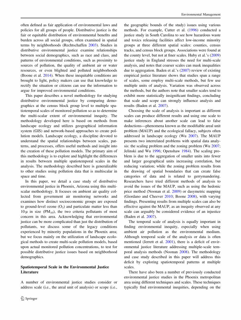
Rasters for the 2008–2010 kriged pollution surface maps foreach temporal extent were averaged together using theRaster Calculator tool in ArcMap, thus creating an averagepollution surface for each extent with a 250 m resolution.These average surfaces were categorized into three spatialscales: the initial pollution surface or raw data, pollutiondeciles, and pollution quartiles (the decile and quartilesurfaces were created with the Reclassify tool in ArcMap).After converting to polygons, these pollution surfaces werespatially joined in a one-to-one relationship with the censusdata using the pollution score at the centroid of each blockgroup; thus each census block group had its centroid-associated pollution value listed. The spatially explicittables were then exported for statistical analysis (Fig. 4).

Table 1 List of agenciesoperating monitoring stationswithin the study area. Agenciessubmit their data to the EPA’sAQS database, which was thesource of data for this study

Agency Type of agency # O3 stations # PM10 stations

Arizona Department of EnvironmentalQuality

State 3 2

Fort McDowell Yavapai Nation Tribal 1 1

Gila River Indian Community Tribal 2 1

Maricopa County Air Quality Department Local (County) 17 14

Pinal County Air Quality Control District Local (County) 5 9

Salt River Pima-Maricopa Indian community Tribal 4 3

Table 2 Details on the temporal scales used within this study

Pollutant Temporal resolution Studyyears

Temporal extents

Ozone 1-h averages, continuoussample grain

2008–2010 Seasonal(Apr–Oct)

Monthly (July) 8-h (15 July,15:00–22:00)

1-h (15 July, 15:00)

PM10 24-h averages, 1-in-6 daysample grain

2008–2010 Annual Monthly (Jan) Monthly (Aug) Daily (Jan)[7 Jan, 2008,7 Jan, 2009,8 Jan, 2010]

Daily (Aug)[22 Aug, 2008,23 Aug, 2009,24 Aug, 2010]

Note that the PM10 daily temporal extent occurs on different days in each of the study years because of the 1-in-6 day sample resolution

Environmental Management

Environmental Management

Statistical Model

We used hierarchical multiple regression models to examinethe independent effects of the four census groups (socio-economic status, age, race, and ethnicity) with each pollu-tion surface at each temporal extent and spatial aggregation.This resulted in a total of 48 and 60 regression equations forO3 and PM10, respectively. Models 1–4 were ordered in thehierarchical multiple regression using an a priori decision ofsocioeconomic status (median household income), age(proportion age≤ 17 and proportion age≥ 65), race (pro-portion African American and proportion Native Amer-ican), and ethnicity (proportion Hispanic) (Table 5; also seeSupplementary Tables S1, S2 in the Supplementary Mate-rials for complete details).

The models were created in SPSS Version 22.0 (IBMCorp 2013). Input data were transformed as necessary, andhomoskedasticity was tested for with Breusch-Pagan andKoenker tests. These tests revealed that data were sig-nificantly heteroskedastic, so the heteroskedasticity-consistent standard error estimator model HC3, run usinga script developed for SPSS by Hayes and Cai (2007), wasused to reduce bias.

Results

The hierarchical multiple regression models did find sig-nificant relationships between the dependent pollution andindependent demographic variables (see Online ResourcesSupplementary Tables S1, S2 for complete statistical

results). These relationships are summarized in Table 6,which is based upon model 4 of the regressions, and iden-tifies those that could possibly be a justice issue, i.e., theindependent variable is a significant predictor for thedependent variable. These positive relationships were notedas possible justice issues based upon the slope of the betascore in the regression, e.g., a negative beta woulddemonstrate a trend of the concentration of pollutionincreasing while the median household income of the cen-sus block group decreases and a positive beta reveals a trendwhere the pollution concentration and the proportion of ademographic group increase together.

There were few instances where changing the temporalscale or spatial aggregation changed significant relation-ships between the dependent and independent variables(Table 6). The examples of this were O3 with the variablesmedian household income and proportion aged≤ 17, andPM10 with income and proportion Hispanic; in all othercases the direction of the effects were the same when sig-nificant relationships were found.

There were many examples where changing scaleresulted in the model 4 relationship becoming non-significant (Table 6). This was especially prevalent in themedian household income variable for both O3 and PM10.In many of these cases, income did act as a significantpredictor for pollution levels in models 1 through 3; how-ever, the addition of the proportion Hispanic independentvariable in model 4 explained away the relationshipbetween pollution and income causing the significant rela-tionship to be lost (Supplementary results SupplementaryTables S1, S2).

There were several distinct consistent patterns thatemerged in the data. At most scales, the proportion ofpeople aged 17 and under was a significant predictor forboth O3 and PM10; however, the proportion of people aged65 and over was only a significant predictor for PM10 andwas negatively correlated with O3. The proportion ofAfrican Americans was a strong predictor for PM10, but hadan equally strong negative relationship with O3. In contrast,the proportion of Native Americans was a predictor for O3,but had a negative relationship with PM10. The proportionof Hispanics had a strong negative correlation with O3, but aless consistent relationship with PM10, with the August

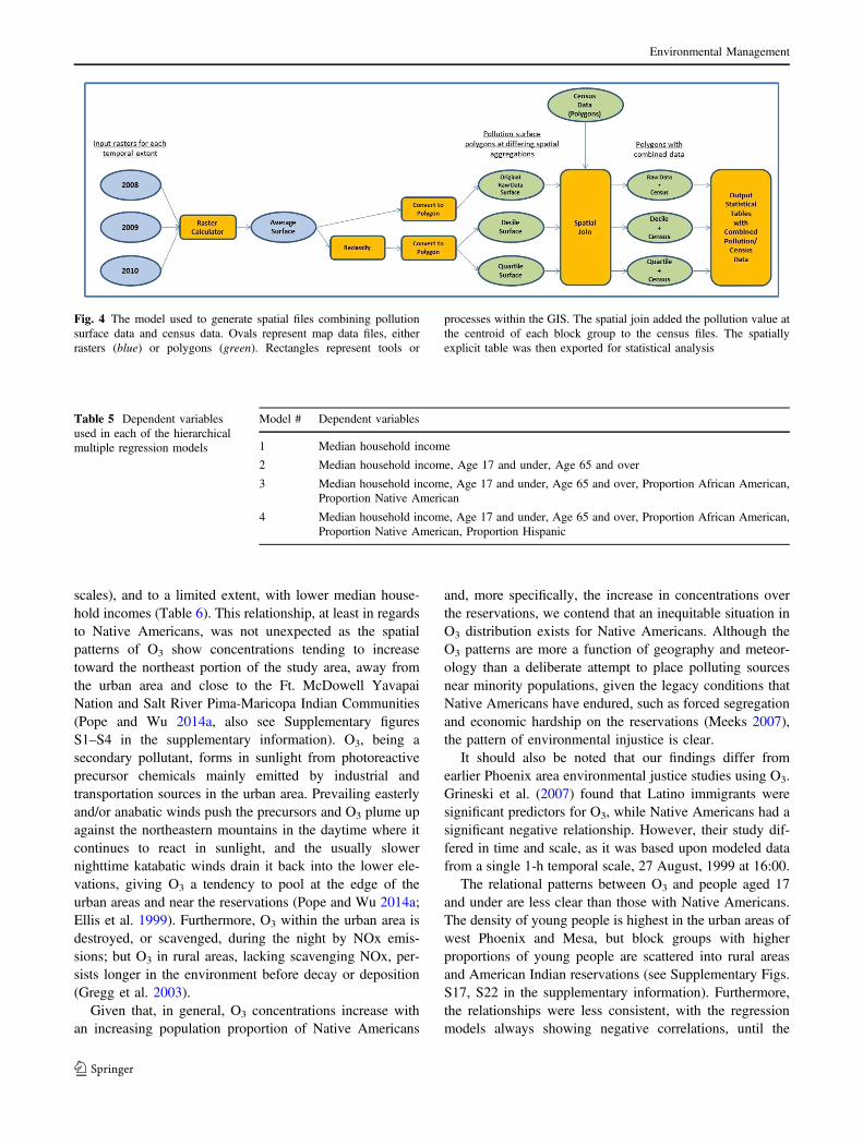
Fig. 2 An example of pollution contours overlaying population pro-portion maps. a Displays O3 pollution contours (with units of PPB)taken at the seasonal temporal extent and averaged from 2008–2010,overlaying the population proportion of Native Americans at thecensus block group level, b is the same map at a finer resolution andfocused upon the metropolitan Phoenix urban area to display details.c Repeats this for PM10 contours (with units of µg/m3) at the annualtemporal extent overlaying the population proportion of AfricanAmericans and d is a finer resolution in the urban metropolitan area.See Supplementary materials, Figs. S1–S9, for complete maps from alltemporal extents

Table 3 Spatial and population statistics for the census block groups located within the O3 and PM10 study areas

Study area Census block groups spatial statistics Census block groups population statistics

N Min. size(km2)

Max. size(km2)

Mean size(km2)

SD (km2) Population N Min. pop. Max. pop. Mean pop. SD

O3 2646 0.085 904.9 4.23 27.36 4,108,844 0 7293 1552.9 698.4

PM10 2172 0.085 603.0 2.91 17.30 3,380,319 0 7293 1556.3 680.9

Note that only block groups that were completely inside the respective study areas were included

Environmental Management

monthly and daily temporal scales varying between posi-tive, negative, and non-significant beta scores (Table 6).

Discussion

Multi-scalar Results

Though changing the temporal scale changed the slope of themodel results, i.e., from negative to positive or vice versa, in

a few instances, the effect was less than anticipated (Table 6).A more common occurrence was to change the relationshipfrom significant to non-significant, or vice versa, between theindependent and dependent variables when the temporalscale was changed. This indicates that, in most cases, eventhough the spatial pattern of the pollutant is visibly changedbetween time periods, the representative relationship betweenpollution sources/dynamics and demographics did notchange. Another interesting result was the change betweenthe PM10 winter and summer scales, especially in relation to

Fig. 3 Map of the census blockgroups that were used within thePM10 and O3 portions of thestudy. Note that only those blockgroups that were fully containedwithin the respective study areaswere included. The very large,sparsely populated block groupsin rural areas that crossed thestudies’ boundaries wereexcluded. Block groups that arecolored light gray were used inthe O3 study, those that arecolored dark gray were used forboth the O3 and PM10 studies

Environmental Management

the Hispanic demographics. These changes in the spatialpattern of PM10 are likely the result of changes in meteor-ology between the seasons, as source apportionment likelyremains the same (Pope and Wu 2014a).

In many of these cases we do not have definitive proofabout the reasons for the change, or lack thereof, of therelationships between demographics and the pattern ofpollutants at differing temporal scales. The spatial patternsof pollutants often do change between the differing timeperiods, so the reasons could range from the new patternsaffecting differing population groups to a blurring hetero-geneity of demographics. However, apparent associationsbetween demographics and the pollution patterns are notedwhere appropriate.

Changes in spatial aggregation of pollutant also resultedin less effect than expected. We expected that aggregatinginto deciles, and especially into quartiles, would bring manychanges from the MAUP scaling problem. In actuality, ofthe 54 regression models, aggregating to deciles changedthe results (including changing to non-significance) fivetimes, or 9 % of the time. Aggregating to quartiles changedthe results a total of 13 times, or 24 % of the time (Table 6).

Environmental Inequity with O3 Pollution

Our analysis shows that significant relationships of possibleenvironmental inequity exists between O3 pollution andNative Americans, youth under 17 years of age (at most

Table 4 Descriptive statistics for study variables, based upon census block groups

O3 study area N Range Min. Max. Mean SD Vari.

Socioeconomic status

Median household income (thousands) 2646 200.0 0.0 200.0 56.9 28.9 834.1

Age proportion

≤Age 17 (%) 2646 59 0 59 25 10 1

≥Age 65 (%) 2646 90 0 90 14 17 3

Race proportion

African American (%) 2646 60 0 60 5 5 0

Native American (%) 2646 98 0 98 2 7 1

Ethnicity proportion

Hispanic (%) 2646 94 0 94 28 24 6

O3 pollution

Seasonal O3 (ppb) 2646 11.6 33.0 44.5 36.9 2.0 4.1

Monthly (July) O3 (ppb) 2646 8.4 35.0 43.4 39.3 1.5 2.3

8-h O3 (ppb) 2646 19.6 33.2 52.8 41.8 4.0 16.3

1-h O3 (ppb) 2646 20.3 46.3 66.6 55.6 5.2 27.4

PM10 study area N Range Min. Max. Mean SD Vari.

Socioeconomic status

Median household income (thousands) 2172 200.0 0.0 200.0 54.4 28.0 782.8

Age proportion

≤Age 17 (%) 2172 59 0 59 26 10 1

≥Age 65 (%) 2172 86 0 86 13 15 2

Race proportion

African American (%) 2172 60 0 60 5 5 0

Native American (%) 2172 98 0 98 3 7 1

Ethnicity proportion

Hispanic (%) 2172 94 0 94 32 24 6

PM10 pollution

Annual PM10 (µg/m3) 2172 74.0 20.7 94.6 30.4 6.9 47.5

Monthly (Jan) PM10 (µg/m3) 2172 34.3 8.2 42.5 20.2 6.4 40.8

Monthly (Aug) PM10 (µg/m3) 2172 57.0 24.0 81.0 31.3 5.3 28.4

Daily (Jan) PM10 (µg/m3) 2172 35.8 10.0 45.8 21.3 6.0 36.1

Daily (Aug) PM10 (µg/m3) 2172 50.3 17.9 68.2 24.7 4.8 23.4

Environmental Management

scales), and to a limited extent, with lower median house-hold incomes (Table 6). This relationship, at least in regardsto Native Americans, was not unexpected as the spatialpatterns of O3 show concentrations tending to increasetoward the northeast portion of the study area, away fromthe urban area and close to the Ft. McDowell YavapaiNation and Salt River Pima-Maricopa Indian Communities(Pope and Wu 2014a, also see Supplementary figuresS1–S4 in the supplementary information). O3, being asecondary pollutant, forms in sunlight from photoreactiveprecursor chemicals mainly emitted by industrial andtransportation sources in the urban area. Prevailing easterlyand/or anabatic winds push the precursors and O3 plume upagainst the northeastern mountains in the daytime where itcontinues to react in sunlight, and the usually slowernighttime katabatic winds drain it back into the lower ele-vations, giving O3 a tendency to pool at the edge of theurban areas and near the reservations (Pope and Wu 2014a;Ellis et al. 1999). Furthermore, O3 within the urban area isdestroyed, or scavenged, during the night by NOx emis-sions; but O3 in rural areas, lacking scavenging NOx, per-sists longer in the environment before decay or deposition(Gregg et al. 2003).

Given that, in general, O3 concentrations increase withan increasing population proportion of Native Americans

and, more specifically, the increase in concentrations overthe reservations, we contend that an inequitable situation inO3 distribution exists for Native Americans. Although theO3 patterns are more a function of geography and meteor-ology than a deliberate attempt to place polluting sourcesnear minority populations, given the legacy conditions thatNative Americans have endured, such as forced segregationand economic hardship on the reservations (Meeks 2007),the pattern of environmental injustice is clear.

It should also be noted that our findings differ fromearlier Phoenix area environmental justice studies using O3.Grineski et al. (2007) found that Latino immigrants weresignificant predictors for O3, while Native Americans had asignificant negative relationship. However, their study dif-fered in time and scale, as it was based upon modeled datafrom a single 1-h temporal scale, 27 August, 1999 at 16:00.

The relational patterns between O3 and people aged 17and under are less clear than those with Native Americans.The density of young people is highest in the urban areas ofwest Phoenix and Mesa, but block groups with higherproportions of young people are scattered into rural areasand American Indian reservations (see Supplementary Figs.S17, S22 in the supplementary information). Furthermore,the relationships were less consistent, with the regressionmodels always showing negative correlations, until the

Fig. 4 The model used to generate spatial files combining pollutionsurface data and census data. Ovals represent map data files, eitherrasters (blue) or polygons (green). Rectangles represent tools or

processes within the GIS. The spatial join added the pollution value atthe centroid of each block group to the census files. The spatiallyexplicit table was then exported for statistical analysis

Table 5 Dependent variablesused in each of the hierarchicalmultiple regression models

Model # Dependent variables

1 Median household income

2 Median household income, Age 17 and under, Age 65 and over

3 Median household income, Age 17 and under, Age 65 and over, Proportion African American,Proportion Native American

4 Median household income, Age 17 and under, Age 65 and over, Proportion African American,Proportion Native American, Proportion Hispanic

Environmental Management

Hispanic demographics were added in model 4 (Supple-mentary Table S1 in the supplementary information). Inaddition, this demographic was one of the few to showdiffering results with a change of temporal scales, and O3 ata monthly scale was either non-significant or negativelycorrelated (Table 6). Thus while it is difficult to pointdirectly to an overall pattern of inequity, there are certainly,on average, locales and temporal scales where youth areexposed to an excessive distribution of O3 pollution.

Environmental Inequity with PM10 Pollution

Our analysis of the relationship between PM10 concentra-tions and independent demographics show patterns that areoften directly opposite to those of O3. At most scales,African Americans, Hispanics, and people aged 65 andolder, while having negative relationships with O3, becamesignificant predictors for PM10. People aged 17 and underwere usually predictors for PM10, except at Januarymonthly scale when the addition of the Hispanic populationto the regression model explained away the relationshipwith youth. As in the O3 analysis, income was an incon-sistent predictor for PM10, especially at the summer tem-poral scales. Lower incomes were usually predictors forPM10 in models 1–3 of the regression, but this relationship

often changed after adding the Hispanic demographic inmodel 4 (Supplementary Table S2 in the Supplementaryinformation).

As with O3, the known characteristics and patterns ofPM10 pollution in Phoenix supports these results. UnlikeO3, PM10 is a primary pollutant that tends to aggregatearound its sources in addition to windblown transport fromthe surrounding desert areas. Many of the PM10 ‘hotspots’in the study area were created from localized sourcesincluding agriculture in rural Pinal county and extractivemining and material handling industries in South Phoenix(Dimitrova et al. 2012; Fernando et al. 2009; Clements et al.2013). In addition, South Phoenix is in the Salt River floodplain and has the lowest average elevations in the metro-politan area. The river channel acts as a natural transportcorridor and downwind sink for early morning particlesemitted from other portions of the metropolitan area(Dimitrova et al. 2012). The South Phoenix area has highproportions of African American and Hispanic populations,though Hispanic populations are more spatially distributedthroughout the study area, and this is likely to account formuch of the correlation in the results.

The spatial correlation between the youth and elder agegroups and PM10 is more difficult to note with visualinspection of the maps. Youth proportions appear to be

Table 6 Summary of hierarchical regression results for Model 4 of the O3 and PM10 parameters and demographic variables at each spatial andtemporal scale

Median household income Proportion age≤ 17 Proportion age≥ 65

Raw data Deciles Quartiles Raw data Deciles Quartiles Raw data Deciles Quartiles

O3 Seasonal + + NS + + NS – – –

Monthly NS NS – NS – – – – –

8-h NS NS NS + + + NS NS NS

1-h NS NS NS + + NS – – –

PM10 Annual – – NS + + + + + +

Jan monthly – – – NS NS NS NS NS +

Jan daily NS – – + + + + + +

Aug monthly NS NS + + + + + + +

Aug daily – NS NS + + + + + +

Proportion African American Proportion Native American Proportion Hispanic

RawData

Deciles Quartiles RawData

Deciles Quartiles RawData

Deciles Quartiles

O3 Seasonal – – – + + + – – –

Monthly – – – + NS + – – –

8 h – – – + + + – – –

1 h – – – + + + – – –

PM10 Annual + + + – – – + + +

Jan monthly + + + – – – + + +

Jan daily + + + – – – + + +

Aug monthly + + + – – – NS NS –

Aug daily + + + – – NS + NS –

NS=No significant relationships found; –=Negative correlation suggesting unlikely inequitable relationship; += Positive correlation suggestingpossible inequitable relationship

Environmental Management

higher through the rural areas and urban fringe, which areareas tending to have higher PM10 concentrations (Sup-plementary Fig. S22 in Online Resource). Elder proportionsare highest in the retirement communities in the northwestportion of the study area (Sun City), east Mesa, and thecenter of the study area (Sun Lakes) (Supplementary Fig.S23 in the Online Resource). PM10 concentrations wererelatively low at all scales in the Sun City area, therefore thecorrelation with PM10 is likely due to the elder populationsliving in Mesa and Sun Lakes.

The spatial pattern, quantified by the statistical results,confirms an inequitable situation between PM10 distributionand African American and Hispanic populations. Legacyconditions with these populations, e.g., historical segrega-tion into South and West Phoenix alongside industrialsource zoning, clarifies the origin of these long-terminequities with minority population in these areas (Bolinet al. 2005).

Limitations

Environmental justice studies, including this study, oftenuse classic regression models to test the relationshipbetween independent and dependent variables (Chakrabortyet al. 2011). The classic global regression model makes twokey assumptions, that observations and residuals are inde-pendent and the process under study is stationary.Assumptions regarding stationarity can be made if theregion under study and the data set are small enough and thespatial units are as small as possible, as in the case of censusblock groups for this study (Gilbert and Chakraborty 2011;Páez 2004; Grineski and Collins 2008). However, thedemographic data used in this study did show clustering, asMoran’s I tests returned significant results for all groups(P< 0.01).

Based on the results shown by changing the spatialaggregation of pollutant data, we believe that stationaritybias in our regression model is low. However, future studiescould be improved by using regression techniques thatcontrol for spatial dependence, such as geographicallyweighted regression or simultaneous autoregressive models(Brunsdon et al. 1999; Kissling and Carl 2008; Chakraborty2009).

It should also be noted that there is inherent spatial errorinvolved in using kriging interpolation to create the pollu-tion surfaces, especially when the density of the input net-work is sparse. Although alternatives have been suggestedto minimize this error, e.g., using linear regression modelsto improve the interpolation (Diem 2003; Diem and Comrie2002), these methods have their own drawbacks includingthe need for significant high-resolution data resources; andthus are best suited to smaller scales.

Though we recognize the inherent problems with kriginginterpolation, we contend that since this study focuses pri-marily on the regional scale pattern and its changes betweentemporal scales, our pollution surfaces are adequately robustfor the purposes. To further test this contention, we createderror prediction surfaces and performed a removal biasanalysis on the interpolated surface (see Online ResourcesSupplementary Figs. S10, S11). This analysis showedestimated average bias for O3 at 2 ppb (Range: 7–0 ppb;SD: 2 ppb). PM10 exhibited more error than O3, with anaverage bias of 11.8 µg/m3 (Range: 91.5–0.1; SD: 18.7).The highest bias existed in sparsely populated rural areaswhere stations are farther apart in distance, and is especiallyassociated with PM10 hotspots located in rural areas southof metropolitan Phoenix. PM10 bias in the metropolitanarea, where monitoring stations, and population, are moredensely located, was considerably lower (see OnlineResource Supplementary Fig. 11).

Conclusions

Distributive environmental inequities exist in the Phoenixarea across spatial scales for the two ambient pollutants ofmost concern—O3 and PM10. These inequities affect dif-ferent social groups to varying degrees, based on theirlocation and population proportion in the metropolitan area.These populations have various legacy stories behind them:Native Americans were forcibly confined to reservations inthe nineteenth century where the greater part of their free-dom and livelihood was denied them (Meeks 2007). AfricanAmericans and Hispanic people, arriving after the nine-teenth century Anglo settlers, were excluded from living inprivileged areas reserved for Whites, including by restric-tive deeds and covenants, and instead were segregated intoSouth and West Phoenix, where city planners placed heavyindustries and waste handling facilities (Bolin et al. 2013).The observed patterns between air pollution and demo-graphics today are in part a persistent legacy of pastsegregation.

Youth and elder populations, most vulnerable to pollu-tion effects, have different situations. The elder population,while certainly not a unique group suffering oppression likeminority populations in the past, has nevertheless oftenpurchased their retirement homes with the expectation of aclean and healthy environment; and the youth are obviouslyunder the authority of their guardians and have little to sayabout the environment where they live. All of these groupshave distinct reasons for being protected from environ-mental inequities, which begins with identifying therelationships.

The occurrence of adverse health effects to these dif-fering population groups because of excessive exposure to

Environmental Management

O3 or PM10 has not been confirmed with this study,although serious health complications can be impliedfrom frequent acute or long-term chronic exposure tothese pollutants (Pope and Dockery 2006; Lippmann1989). The case to be made here is that conditions, eitherhistorical or current, are such that populations of limitedmobility are located in areas where they bear a largerburden of criteria pollutant exposure. Our findings canhelp policy makers and regulating agencies in the Phoenixarea to make more informed decisions to protect the healthof its communities.

Our case study has shown the usefulness of using amulti-scaled spatiotemporal methodology for investigatingenvironmental justice issues. This methodology is gen-eralizable to other studies where pollution data, especiallyambient air pollution data, from a network or model existsacross multiple scales of space and time. As shown in thiscase study, air pollution patterns are spatially hetero-geneous and temporally dynamic, so the utilization of amulti-scaled spatiotemporal methodology is important todiscover the full extent of distributive environmentalinequity.

Acknowledgments We are grateful to the three anonymousreviewers who provided excellent comments to help strengthen ourmanuscript.

Compliance with ethical standards

Conflict of interest The authors declare that they have no conflict ofinterest.

References

Andersen ZJ, Wahlin P, Raaschou-Nielsen O, Scheike T, Loft S(2007) Ambient particle source apportionment and daily hospitaladmissions among children and elderly in Copenhagen. J ExpoSci Environ Epidemiol 17(7):625–636

Baden BM, Noonan DS, Turaga RMR (2007) Scales of justice: is therea geographic bias in environmental equity analysis?. J EnvironPlann Manag 50(2):163–185

Bolin B, Barreto JD, Hegmon M, Meierotto L, York A (2013) Doubleexposure in the sunbelt: The sociospatial distribution of vulner-ability in Phoenix, Arizona. In: Boone C, Fragkias M (eds)Urbanization and sustainability: Linking urban ecology, envir-onmental justice and global environmental change. Springer, TheNetherlands, pp. 159-178.

Bolin B, Grineski S, Collins T (2005) The Geography of Despair:Environmental Racism and the Making of South Phoenix, Ari-zona, USA. Hum Ecol Rev 12(2):156–168

Bolin B, Matranga E, Hackett EJ, Sadalla EK, Pijawka KD, Brewer D,Sicotte D (2000) Environmental equity in a sunbelt city: thespatial distribution of toxic hazards in Phoenix, Arizona. EnvHazards 2:11–24

Bolin B, Nelson A, Hackett EJ, Pijawka KD, Smith CS, Sicotte D,Sadalla EK, Matranga E, O’Donnell M (2002) The ecology oftechnological risk in a Sunbelt city. Env Plan 34:317–339

Boone CG (2008) Improving resolution of census data in metropolitanareas using a dasymetric approach: Applications for the BaltimoreEcosystem Study. Cities Env 1(1):3. doi:http://digitalcommons.lmu.edu/cate/vol1/iss1/3

Boone CG, Fragkias M, Buckley GL, Grove JM (2014) A long view ofpolluting industry and environmental justice in Baltimore. Cities36(0):41–49. doi:http://dx.doi.org/10.1016/j.cities.2013.09.004

Brulle RJ, Pellow DN (2006) Environmental Justice: Human Healthand Environmental Inequalities. Annu Rev Public Health27(1):103–124

Brunsdon C, Fotheringham AS, Charlton M (1999) Some Notes onParametric Significance Tests for Geographically WeightedRegression. J Reg Sci 39(3):497–524

Bullard RD (1990) Dumping in Dixie: Race, Class, and EnvironmentalQuality. Westview Press, Boulder, CO

Chakraborty J (2009) Automobiles, Air Toxics, and Adverse HealthRisks: Environmental Inequities in Tampa Bay, Florida. AnnAssoc Am Geogr 99(4):674–697

Chakraborty J, Maantay JA, Brender JD (2011) DisproportionateProximity to Environmental Health Hazards: Methods, Models,and Measurement. Am J Public Health 101(S1):S27–S36

Clements AL, Fraser MP, Upadhyay N, Herckes P, Sundblom M,Lantz J, Solomon PA (2013) Characterization of summertimecoarse particulate matter in the Desert Southwest—Arizona,USA. J Air Waste Manag Assoc 63(7):764–772. doi:10.1080/10962247.2013.787955

Cressie N (1990) The Origins of Kriging. Math Geol 22(3):239–252Cutter SL, Holm D, Clark L (1996) The Role of Geographic Scale in

Monitoring Environmental Justice. Risk Analysis 16(4):517–526Cutter SL, Solecki WD (1996) Setting environmental justice in space

and place: Acute and chronic airborne toxic releases in thesoutheastern United States. Urban Geography 17(5):380–399

Diem JE (2003) A critical examination of ozone mapping from aspatial-scale perspective. Environ Pollut 125(3):369–383

Diem JE, Comrie AC (2002) Predictive mapping of air pollutioninvolving sparse spatial observations. Environ Pollut 119(1):99–117

Dimitrova R, Lurponglukana N, Fernando HJS, Runger GC, Hyde P,Hedquist BC, Anderson J, Bannister W, Johnson W, Baklanov A(2012) Relationship between particulate matter and childhoodasthma—basis of a future warning system for central Phoenix.Atmos Chem Phys 12(5):2479–2490

Ellis AW, Hildebrandt ML, Fernando HJS (1999) Evidence of lower-atmospheric ozone “sloshing” in an urbanized valley. Phys Geogr20(6):520–536

ESRI (2010) ArcMap Version 10.0. ESRI (Environmental SystemsResource Institute), Redlands, CA

Fernando HJS, Dimitrova R, Runger G, Lurponglukana N, Hyde P,Hedquist B, Anderson J (2009) Children’s health project: Linkingasthma to PM10 in central Phoenix – a report to the Arizonadepartment of environmental quality. Arizona State University’sCenter for Environmental Fluid Dynamics and Center for HealthInformation and Research. http://www.azdeq.gov/ceh/download/Health%20Project%20Report.pdf. Accessed 26 Feb 2014.

Fortin MJ, Dale MRT (2005) Spatial Analysis: A Guide for Ecologists.Cambridge University Press, Cambridge, UK

Gamma Design Software (2006) GS+: Geostatistics for the Environ-mental Sciences, 7.0 (Build 25) edn. Gamma Design Software,Plainwell, Michigan, USA

Gilbert A, Chakraborty J (2011) Using geographically weightedregression for environmental justice analysis: Cumulative cancerrisks from air toxics in Florida. Soc Sci Res 40(1):273–286

Giordano A, Cheever L (2010) Using dasymetric mapping to identifycommunities at risk from hazardous waste generation in SanAntonio, Texas. Urban Geogr 31(5):623–647

Environmental Management

Gregg JW, Jones CG, Daws TE (2003) Urbanization effects on treegrowth in the vicinity of New York City. Nature 424:183–187

Grineski S (2007) Incorporating health outcomes into environmentaljustice research: the case of children’s asthma and air pollution inPhoenix, Arizona. Env Hazards 7:360–371

Grineski S, Bolin B, Boone C (2007) Criteria air pollution and mar-ginalized populations: environmental inequity in metropolitanPhoenix, Arizona. Soc Sci Q 88 (2).

Grineski SE, Collins TW (2008) Exploring patterns of environmentalinjustice in the global south: “Maquiladoras” in Ciudad Juárez,Mexico. Popul Environ 29(6):247–270

Hayes A, Cai L (2007) Using heteroskedasticity-consistent standarderror estimators in OLS regression: An introduction and softwareimplementation. Behav Res Methods 39(4):709–722

Huby M, Cinderby S, White P, Bruin Ad (2009) Measuring inequalityin rural England: the effects of changing spatial resolution.Environ Plann A 41(12):3023–3037

IBM Corp (2013) IBM SPSS Statistics for Windows, 22.0 edn. IBMCorp, Armonk, NY

Jelinski DE, Wu JG (1996) The modifiable areal unit problem andimplications for landscape ecology. Landscape Ecol 11(3):129–140

Jerrett M, Burnett RT, Kanaroglou P, Eyles J, Finkelstein N, Giovis C,Brook JR (2001) A GIS—environmental justice analysis of par-ticulate air pollution in Hamilton, Canada. Environ Plann A 33(6):955–973

Kissling WD, Carl G (2008) Spatial autocorrelation and the selectionof simultaneous autoregressive models. Global Ecol Biogeogr 17(1):59–71

Lippmann M (1989) Health Effects of Ozone; A Critical Review.JAPCA 39(5):672–695

Meeks EV (2007) Border citizens: the making of Indians, Mexicans,and Anglos in Arizona. University of Texas Press, Austin, Texas

Mohai P, Saha R (2007) Racial inequality in the distribution ofhazardous waste: a national-level reassessment. Soc Probl 54(3):343–370. doi:10.1525/sp.2007.54.3.343

Noonan DS (2008) Evidence of environmental justice: a critical per-spective on the practice of EJ research and lessons for policydesign. Soc Sci Q 89(5):1153–1174

Noonan DS, Turaga RM, Baden BM (2009) Superfund, hedonics,and the scales of environmental justice. Environ Manage 44(5):909–920

Openshaw S (1984) The Modifiable Areal Unit Problem. Geo Books,Norwich

Páez A (2004) Anisotropic variance functions in geographicallyweighted regression models. Geogr Anal 36(4):299–314

Pope CA, Dockery DW (2006) Health effects of fine particulate airpollution: lines that connect. J Air Waste Manag Assoc 56(6):709–742

Pope RL, Wu J (2014a) Characterizing air pollution patterns onmultiple time scales in urban areas: a landscape ecologicalapproach. Urban Ecosyst 17(3):855–874. doi:10.1007/s11252-014-0357-0

Pope RL, Wu J (2014b) A multi-objective assessment of an air qualitymonitoring network using environmental, economic, and socialindicators and GIS-based models. J Air Waste Manag Assoc 64(6):721–737. doi:10.1080/10962247.2014.888378

Rechtschaffen C (2003) Advancing environmental justice norms. UCDavis L Rev 37:95

Tecer LH, Alagha O, Karaca F, Tuncel G, Eldes N (2008) Particulatematter (PM2.5, PM10-2.5, and PM10) and children’s hospitaladmissions for asthma and respiratory diseases: a bidirectionalcase-crossover study. J Toxicol Environ Health, Part A 71(8):512–520

U.S. EPA (2015) The Green Book Non-Attainment Areas for CriteriaPollutants. Environmental Protection Agency. http://www.epa.gov/oaqps001/greenbk/index.html. Accessed 25 March2015.

United Church of Christ (UCC) (1987) Toxic wastes and race inthe United States: a national report on the racial andsocio-economic characteristics of communities with hazardouswaste sites. United Church of Christ, Commission for RacialJustice, New York

Williams RW (1999) The contested terrain of environmental justiceresearch: community as unit of analysis. Soc Sci J 36(2):313–328.doi:http://dx.doi.org/10.1016/S0362-3319(99)00008-7

Wu J (2007) Scale and scaling: A cross-disciplinary perspective. In:Wu JG, Hobbs RJ (eds) Key topics in landscape ecology. Cam-bridge University Press, Cambridge, UK, pp. 115-142.

Wu J, Jenerette GD, Buyantuyev A, Redman CL (2011) Quantifyingspatiotemporal patterns of urbanization: the case of the two fastestgrowing metropolitan regions in the United States. Ecol Complex8(1):1–8

Environmental Management