spatial dynamic patterns of hand-foot-mouth disease in the ... jf-hfmd geospatial health.pdf ·...

Spatial dynamic patterns of hand-foot-mouth disease in thePeople’s Republic of China

Jin-Feng Wang1, Cheng-Dong Xu1, Shi-Lu Tong2, Hong-Yan Chen3, Wei-Zhong Yang4

1State Key Laboratory of Resources and Environmental Information Systems, Institute of Geographic Sciencesand Natural Resources Research, Chinese Academy of Sciences, Beijing, People’s Republic of China; 2School ofPublic Health and Institute of Health and Biomedical Innovation, Queensland University of Technology,Brisbane, Australia; 3School of Environmental Sciences, University of Liverpool, Liverpool, United Kingdom;4Office for Disease Control and Emergency Response, Chinese Center for Disease Control and Prevention,Beijing, People’s Republic of China

Abstract. Hand-foot-mouth disease (HFMD) is the most common and widespread infectious disease in the People’s Republicof China. Although there has been a substantial increase of HFMD in many parts of the country in recent years, its spatialdynamics and determinants remain unclear. When we collected and analysed weekly data on HFMD cases from 1,456 coun-ties and the corresponding meteorological factors from 1 May 2008 to 27 March 2009, it was found that HFMD was spa-tially dispersed across the country in the summer and winter, while clustered in the spring and autumn. The spatial varia-tion of HFMD was found to be affected by a combination of climate variables, while its spatio-temporal transmission waslargely driven by temperature variations with a 7-week lag implying that (i) the dispersal of the disease can be anticipatedbased on the variation of the temperature and other climate variables; and (ii) the spatial dynamics of HFMD can be robust-ly predicted 7 weeks ahead of time using temperature data only. The findings reported allow prompt preparation and imple-mentation of appropriate public health interventions to control and prevent disease outbreaks.

Keywords: hand-foot-mouth disease, spatial dynamic, spatio-temporal transmission, People's Republic of China.

Introduction

Hand-foot-mouth disease (HFMD) is a human syn-drome including fever, blister-like sores in the mouthand a skin rash caused by intestinal viruses of thepicornaviridae family, most commonly coxsackie Avirus or enterovirus 71 (EV-71) (http://www.cdc.gov/hand-foot-mouth/). With 0.5-1 million report-ed cases annually, HFMD is the most frequent andwide spread infectious disease in the People’s Republicof China (P.R. China). A number of epidemiologicalstudies have been conducted to investigate its trans-mission parameters and identify pathogens across dif-

ferent time periods and in different locations (Hii etal., 2011; Wang et al., 2011a; Zhang et al., 2011).Previous studies have shown that the disease is a mod-erately transmittable infectious disease with an effec-tive reproduction (the average number of secondarycases caused by each case, during the infectious peri-od) of approximately 1.4, mainly among preschool-aged children. A higher risk of transmission is associ-ated with temperatures in the range of 21°C to 27°C,high relative humidity, low wind speed, high precipita-tion, high population density and periods duringwhich schools are open (Wang et al., 2011a). Spatio-temporal HFMD clusters, closely linked to the month-ly precipitation, have been found in P.R. China (Wanget al., 2011a). In Singapore, there is normally a 1-2week delay in the incidence of HFMD in response toweekly temperature changes and rainfall (Hii et al.,2011). However, the spatial pattern of the disease isnot yet fully understood.

The spatio-temporal features of an infectious diseaseis usually driven by determinants, which can provideinvaluable information for exploring the risk factorsof the disease and contribute to developing effectivemeasures to control and prevent its transmission(Christakos, 2005; Wang et al., 2011a). Spatio-tempo-ral analysis is increasingly used in epidemiological

Corresponding authors:Jin-Feng WangLREIS, Institute of Geographic Sciences and Natural Resources Research, Chinese Academy of SciencesBeijing, 100101, People’s Republic of ChinaTel. +86 10 6488 8965 Fax +86 10 6488 9630E-mail: [email protected]

Wei-Zhong YangOffice for Disease Control and Emergency ResponseChinese Center for Disease Control and PreventionBeijing 100050, People’s Republic of ChinaTel. +86 10 8315 2988 Fax +86 10 5890 0575E-mail: [email protected]

Geospatial Health 7(2), 2013, pp. 381-390

J-F. Wang et al. - Geospatial Health 7(2), 2013, pp. 381-390

Fig. 1. Distribution of HFMD cases in P.R. China in May 2008.

research based on specific or routinely collected datafrom different sources (Kulldorff, 1997; Haining,2003; Riley, 2008). In a previous study, we used the“self organization mapping-Bayesian maximumentropy” (S-BME) technique (Christakos andHristopulos, 1998; Kolovos et al., 2010) to explorethe relationship between HFMD transmission and cli-mate types on a moderate spatial scale (Wang et al.,2011). However, this approach appeared to overlycompress the spatio-temporal information, sometimesmasking spatio-temporal trends resulting in loss ofcritical information regarding the transmission process(Wang et al., 2011a). We applied the mass centremethod (Wang, 2009) and Moran’s I (Moran, 1950)to datasets of HFMD incidence and climatic drivers todescribe their spatial distribution and spatial cluster-ing at each “time slice” in a series of temporal data toillustrate the spatial dynamics of disease transmission.The purpose was to explore the spatio-temporal asso-ciation between disease transmission and climate vari-ation and to discuss policy implications with respect tointervention.

Materials and methods

We focused on 1,456 counties in the East becausethe western part of P.R. China is sparsely inhabited(Fig. 1). These counties comprise 90% of the nation’spopulation. Between 1 May 2008 and 27 March2009, the average incidence of HFMD was 834.1 per100,000 in these areas (Chinese Center for DiseaseControl and Prevention, Beijing). We collected theweekly average numbers of HFMD cases in the 1,456counties as well as the weekly averages of the meteor-ological variables (the mean, maximum and minimumtemperatures, air pressure, humidity, wind speed, pre-cipitation and hours of sunshine). The disease datawere reported by the county hospitals to the ChineseCenter for Disease Control and Prevention, while theclimate information was provided by the ChineseMeteorological Data Sharing Service System. Theweekly averages of the meteorological variables werecalculated based on the daily values recorded at 676weather stations across the 1,456 counties.

Raw data usually contain too much noise to display

382


Fig. 2. Flow-chart of the study.

Time series

Disease (y)

Spatial patterns

Time series ofspatial patterns

Time series ofHFMD spatial mass

centres

Association (f)

Association between thetwo time series of HFMD

and climate(Fréchet distance)

Explanatory variables (x)

Time series of climate spatial mass

centres

Spatial strata of HFMD incidence

Interaction between clima-te factors leading to

HFMD (geographical detector)

Spatial strata of climate indicators

Time series of spatial clustering of HFMD (Moran’s I; wavelet)

Comparison

Time series of spatial clustering of climate

indicators(Moran’s I; wavelet)

a pattern of a dynamic phenomenon. Conventionalstatistics, time series or spatial statistics are thereforeoften used to describe point estimates with either atemporal or a spatial domain deriving the features ofthe phenomenon in question from the analysis. Spatio-temporal statistics is becoming a mainstreamapproach to investigate the transmission and dispersalof infectious diseases (Riley, 2008; Zhou, 2009;Christakos, 2010; Wang et al., 2011a; Yu et al., 2011).However, because spatio-temporal processes are inte-grated and based on data from all domains, the studyof a single domain would neglect information from theother domains. In the current study, spatial dynamicsof both case and cluster distributions were examinedby a series of spatial mass centres of and Moran’s I sta-tistic values. The association between HFMD with asingle factor (first row in Fig. 2) and their interaction(second row in Fig. 2) were tested by the Fréchet dis-tance approach (Alt and Godau, 1995) and the geo-graphical detector method (Wang et al., 2010b, Wangand Hu, 2012) (Fig. 2) comparing the time series ofspatial clustering of HFMD and climate variables(third row in Fig. 2).

The Fréchet distance is the measure of similaritybetween two curves. This method takes into account thelocation and ordering of the points along the curves. Apopular illustration of the Fréchet distance of twocurves is the following: suppose a man (symbolizing thedriving force of a disease) walking (spatial dynamics)his dog (the disease) on a leash (the association betweenthe disease and its driving force); the man (the force) iswalking (moving forward) along one curve (time series

of the driver) and the dog (spatial dynamics of the dis-ease) on another curve (time series of the disease). Seenin this way, the Fréchet distance is the shortest length ofthe leash (association) allowing them (the determinantand disease) to be on two separate curves from start tofinish. Given two curves, f: [a, a’] V, g: [b, b’] V,δF(f, g), where V stands for a Euclidean vector space,their Fréchet distance is defined as:

where α(0) = a, α(1) = a’, β(0) = b and β(1) = b’. Thefactor δF is obviously symmetric and the triangleinequality holds; the two curves are equivalent if thedistance between them is zero (Alt and Godau, 1995).Two curves with different lengths [a, a’] and [b, b’] arestandardised into the same length [0, 1], by two trans-fer functions α and β, with a parameter t ∈ [0, 1], thevalues of the two curves f and g are then coordinatedby α(t) and β(t) respectively, and their difference meas-ured by δF(f, g) as defined by the equation above. Thediscrete Fréchet distance provides a good approxima-tion of the continuous measure and can be efficientlycomputed using a simple algorithm (Eiter andMannila, 1994). The similarity between two curves isdetermined by the equation:

383

δF(f, g) = infα[0, 1][a, a’]

max || f(α(t)) - g(β(t)) ||t ∈ [0, 1]

β[0, 1][b, b’]

SI(f, g) = 1 -

infα[0, 1][a, a’]

max || f(α(t)) - g(β(t)) ||t ∈ [0, 1]

β[0, 1][b, b’]

supα[0, 1][a, a’]

max || f(α(t)) - g(β(t)) ||t ∈ [0, 1]

β[0, 1][b, b’]


where SI(f, g) ∈ [0, 1]. A value near 1 indicates moresimilarity between the two curves, while a value near 0indicates less similarity between them. I standardizes δF

into [0. 1] in order to facilitate determining the degreeof similarity between two curves in the limited bound.

The degree of global spatial data clustering wasmeasured using Moran’s I coefficient (Moran, 1950).The value of a Moran’s I lies between -1 and 1, wherethe value near +1.0 indicates clustering of HFMDincidence or climate indictors, while -1.0 indicatesspatial dispersal. Spatial clustering at time t wasobtained by:

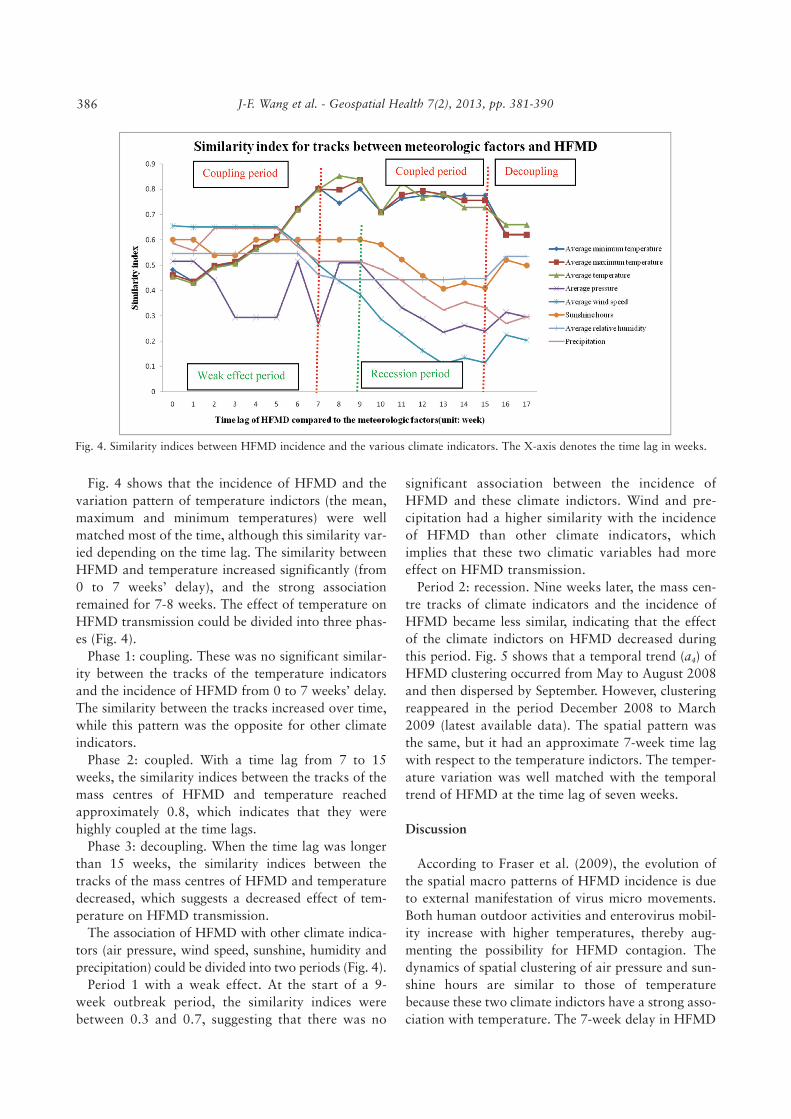
where yi(t) is HFMD incidence or climate indictorsobserved at location i in week t, y– the mean of aquantity such as the number of cases or a climateindicator averaged over the country in the t-thweek, and wij is the weight between two locationscalculated by the inverse distance square method.The time series of I(t) was often noisy, so it was fil-tered using a discrete wavelet transformation imple-mented by the Matlab computer library withDaubechies db3 as the mother-wave and fourdecomposition levels (http://www.mathworks.com).The time series was thus decomposed into low-fre-quency components (a1, a2, a3, a4), reflecting theirfundamental trend, and high frequency components(d1, d2, d3, d4) reflecting the noise caused by randomfactors. The wavelet principle is explained by Fig. 5,where Moran’s I of HFMD is decomposed into a1

and d1; the trend of a1 first not being clarified so itis further decomposed into a2 and d2 and so on untilwe reach a4, in which the low frequency component(a4) clearly displays the spatial dispersion fromAugust until late November. The wavelet decompo-sition of climate indicators in Fig. 5 can be inter-preted in a similar way. The red lines mark the low-est spatial clustering of HFMD (in late November)and of the major climate indicators (in October),respectively.

A disease will exhibit a spatial distribution similar tothat of an environmental factor, if the environmentalattribute leads to the disease. This maxim has generat-ed the geographical detector (Wang et al., 2010b) thatcan be applied for incidence prediction, since peopleliving in different climate strata may have distinctlydifferent incidences of HFMD. The geographicaldetector is grounded on the power of determinant

(PD), which generates four detectors (Wang et al.,2010b) as follows from the equation:

where ℜ and σ 2 denote the area and the variance ofdisease incidence of the study area, respectively. Thestudy area is stratified into L strata, denoted by h =1, …, L (Wang et al., 2010a), according to spatialheterogeneity (defined as an attribute of which sta-tistical properties, e.g. mean and standard deviationor change in space) of a suspected determinant or itsproxy of the disease. PD ∈ [0, 1] means that PD canvary between 1 (the determinant completely controlsthe disease) and 0 (the determinant is completelyunrelated to the disease). Therefore, the PD reflectsthe degree to which a determinant explains the dis-ease prevalence. The geographical detector examineswhether two health determinants, A and B, togetherweaken or enhance one another, or whether they areindependent in contributing to the development of adisease. The interaction between these two determi-nants can be justified by comparing the sum of dis-ease contribution of two individual attributes withthe contribution of the two attributes when com-bined, i.e.

They enhance if PD(A∩B) >PD(A) or PD(B)

They enhance (bivariate) if PD(A∩B) >PD(A) and PD(B)

They enhance (nonlinear) if PD(A∩B) >PD(A) + PD(B)

They weaken if PD(A∩B) <PD(A) + PD(B)

They weaken (univariate) if PD(A∩B) <PD(A) or PD(B)

They weaken (nonlinear) if PD(A∩B) <PD(A) and PD(B)

They are independent if PD(A∩B) = PD(A) + PD(B)

where the interaction (symbolised by ∩) can easily beimplemented in a geographical information system(GIS) by overlaying the two factor layers A and B. Thegeographical detector approach was implemented byusing a computer package available athttp://www.sssampling.org/geogdetector (Wang andHu, 2012).

Results

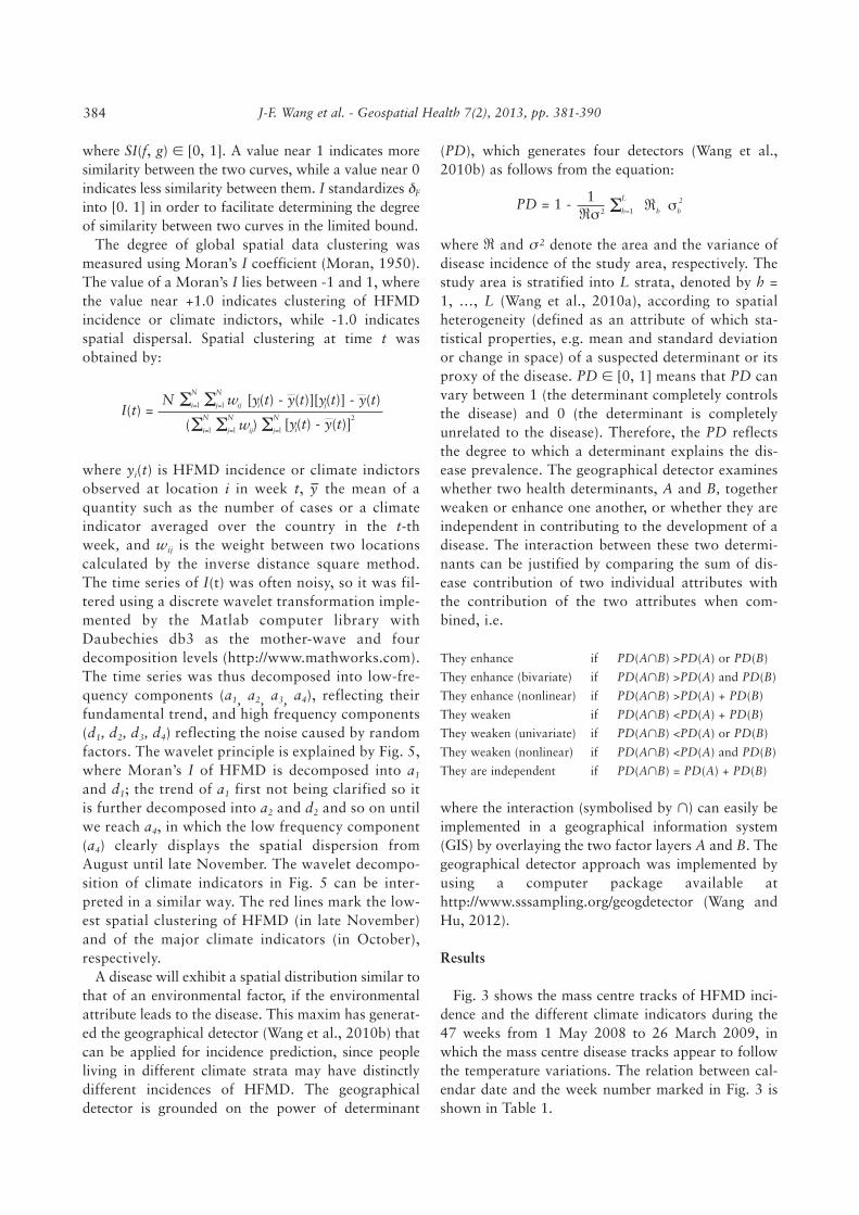
Fig. 3 shows the mass centre tracks of HFMD inci-dence and the different climate indicators during the47 weeks from 1 May 2008 to 26 March 2009, inwhich the mass centre disease tracks appear to followthe temperature variations. The relation between cal-endar date and the week number marked in Fig. 3 isshown in Table 1.

384

I(t) =ΣN w [y(t) - y(t)][y(t)] - y(t)

N

i=l ΣN

j=l ij i j

Σ( )w [y(t) - y(t)]N

i=l ΣN

j=l ΣN

j=lij i

2

PD = 1 - 1ℜσ ΣL

h=12

hh2 ℜ σ


Fig. 3. HFMD mass centre movements and the climate indicators during the 47-week period (numbers correpond to the weeks ofTable 1).

Table 1. Correspondence between week number of the study period and calender date.

Week

Date*

1

2008-5-1

2

2008-5-8

3

2008-5-15

4

2008-5-22

5

2008-5-29

6

2008-6-5

7

2008-6-12

8

2008-6-19

9

2008-6-26

10

2008-7-3

Week

Date*

11

2008-7-10

12

2008-7-17

13

2008-7-24

14

2008-7-31

15

2008-8-7

16

2008-8-14

17

2008-8-21

18

2008-8-28

19

2008-9-4

20

2008-9-11

Week

Date*

21

2008-9-18

22

2008-9-25

23

2008-10-2

24

2008-10-9

25

2008-10-16

26

2008-10-23

27

2008-10-30

28

2008-11-6

29

2008-11-13

30

2008-11-20

Week

Date*

31

2008-11-27

32

2008-12-4

33

2008-12-11

34

2008-12-18

35

2008-12-25

36

2009-1-1

37

2009-1-8

38

2009-1-15

39

2009-1-22

40

2009-1-29

Week

Date*

41

2009-2-5

42

2009-2-12

43

2009-2-19

44

2009-2-26

45

2009-3-5

46

2009-3-12

47

2009-3-19

*yyyy-mm-dd

385


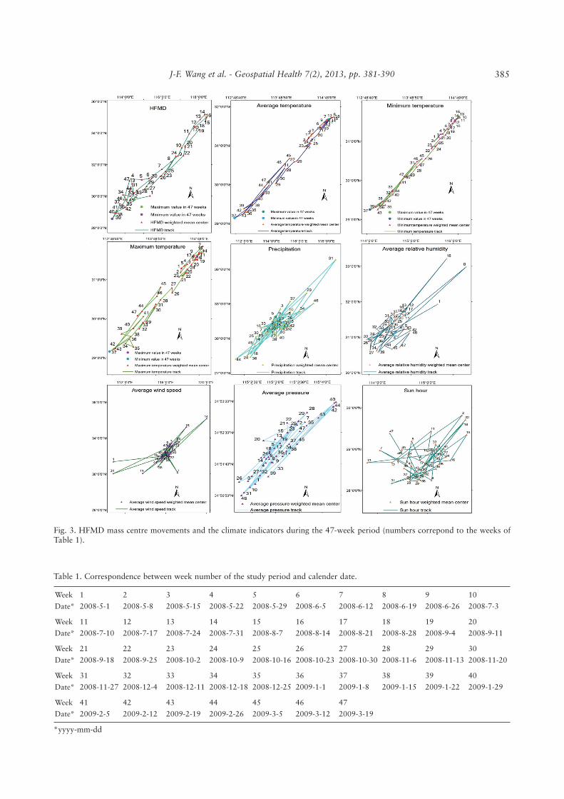
Fig. 4. Similarity indices between HFMD incidence and the various climate indicators. The X-axis denotes the time lag in weeks.

Fig. 4 shows that the incidence of HFMD and thevariation pattern of temperature indictors (the mean,maximum and minimum temperatures) were wellmatched most of the time, although this similarity var-ied depending on the time lag. The similarity betweenHFMD and temperature increased significantly (from0 to 7 weeks’ delay), and the strong associationremained for 7-8 weeks. The effect of temperature onHFMD transmission could be divided into three phas-es (Fig. 4).

Phase 1: coupling. These was no significant similar-ity between the tracks of the temperature indicatorsand the incidence of HFMD from 0 to 7 weeks’ delay.The similarity between the tracks increased over time,while this pattern was the opposite for other climateindicators.

Phase 2: coupled. With a time lag from 7 to 15weeks, the similarity indices between the tracks of themass centres of HFMD and temperature reachedapproximately 0.8, which indicates that they werehighly coupled at the time lags.

Phase 3: decoupling. When the time lag was longerthan 15 weeks, the similarity indices between thetracks of the mass centres of HFMD and temperaturedecreased, which suggests a decreased effect of tem-perature on HFMD transmission.

The association of HFMD with other climate indica-tors (air pressure, wind speed, sunshine, humidity andprecipitation) could be divided into two periods (Fig. 4).

Period 1 with a weak effect. At the start of a 9-week outbreak period, the similarity indices werebetween 0.3 and 0.7, suggesting that there was no

significant association between the incidence ofHFMD and these climate indictors. Wind and pre-cipitation had a higher similarity with the incidenceof HFMD than other climate indicators, whichimplies that these two climatic variables had moreeffect on HFMD transmission.

Period 2: recession. Nine weeks later, the mass cen-tre tracks of climate indicators and the incidence ofHFMD became less similar, indicating that the effectof the climate indictors on HFMD decreased duringthis period. Fig. 5 shows that a temporal trend (a4) ofHFMD clustering occurred from May to August 2008and then dispersed by September. However, clusteringreappeared in the period December 2008 to March2009 (latest available data). The spatial pattern wasthe same, but it had an approximate 7-week time lagwith respect to the temperature indictors. The temper-ature variation was well matched with the temporaltrend of HFMD at the time lag of seven weeks.

Discussion

According to Fraser et al. (2009), the evolution ofthe spatial macro patterns of HFMD incidence is dueto external manifestation of virus micro movements.Both human outdoor activities and enterovirus mobil-ity increase with higher temperatures, thereby aug-menting the possibility for HFMD contagion. Thedynamics of spatial clustering of air pressure and sun-shine hours are similar to those of temperaturebecause these two climate indictors have a strong asso-ciation with temperature. The 7-week delay in HFMD

386


Fig. 5. Wavelet decomposition of Moran’s I values of HFMD and climate indicators (the red lines mark the lowest spatial clusteringof HFMD in late November and of the major climate indicators in October, respectively).

a

b

c

d

e

387


State Interval

A: Temperature variation

B: HFMD enterovirus responses to temperature variation

C: Population response to HFMD enterovirus variation

D: Population infected but in a latent phase

E: Infected person showing symptoms

F: Symptoms becoming obvious enough to make the infectedvisit a clinic where he/she is recorded by the national diseasenotification system.

Table 2. States and intervals from the point of climate variation to the disease response.

a(Goh et al., 1982; Garner and Lack, 1995); b(Alsop et al., 1960; Chang et al., 2002); c(Alsop et al., 1960); d(Wang et al., 2011).

}}}}}

The lag between states A and B still unclear

The lag between states B and C still unclear

The lag between states C and D still unclear

The lag between states D and E is 1 weeka, 1-7 daysb or 5-6 daysc

The lag between states E and F for severe cases is ≥5 daysd

Year/monthClimate factors

A B C A∩B A∩C B∩C

2008-05

2008-06

2008-07

2008-08

2008-09

2008-10

2008-11

2008-12

2009-01

2009-02

2009-03

0.043

0.040

0.017

0.015

0.026

0.010

0.029

0.015

0.045

0.028

0.060

0.119

0.049

0.019

0.031

0.112

0.089

0.111

0.025

0.069

0.104

0.087

0.041

0.049

0.012

0.090

0.054

0.042

0.017

0.017

0.022

0.040

0.102

0.178

0.144

0.103

0.219

0.460

0.194

0.315

0.138

0.263

0.226

0.311

0.141

0.116

0.077

0.316

0.307

0.157

0.131

0.131

0.184

0.141

0.257

0.201

0.169

0.088

0.352

0.347

0.197

0.320

0.116

0.220

0.262

0.248

Table 3. Climate indicators associated with HFMD transmission.

A = monthly average precipitation; B = monthly average temperature; C = monthly total solar radiation; ∩ = interaction.

temperature response is composed of five temporalintervals between six sequential states (Table 2). Atany particular temporal cross-section, some area isdominated by either one of the states.

We examined whether there are interactionsbetween monthly temperature, precipitation, and totalsolar radiation, and their effect on HFMD spatialtransmission. Table 3 shows that the PD values of aninteraction between any two of the climate indicatorsare larger than any single value, which suggests thatthe climate indicators interact and enhance their effecton the spatial transmission of HFMD. The interactionbetween temperature and other climate indicators hada significantly greater effect than any other interactionon spatial transmission of HFMD. The PD values ofclimate in spring and autumn were higher than thosein summer and winter. This finding indicates that spa-tially stratified non-homogeneity of climate in springand autumn strongly controls the spatial dynamics ofHFMD. Also, the disease transmission is less sensitive

to climate change during the summer and winter thanin the spring and autumn.

The statistical approach is good at summarizingthe features of spatio-temporal phenomena and alsofor interpolating the processes based on spatio-tem-poral autocorrelation. However, it is limited withrespect to the understanding of the physical mecha-nism at work and also limited with regard to inter-pretation of the biological principle of the 7-weekdelay of HFMD transmission with temperature vari-ation. Mathematical modelling of a disease process,including the mechanism of transmission, can beemployed to extract epidemiological parameters(Wang et al., 2006, 2011a), and it has been success-fully applied to simulate scenarios under differentcontrolling strategies for many diseases, such asmouth-foot disease (Keeling et al., 2003), influenza(Ferguson et al., 2005) and smallpox (Riley andFerguson, 2006). The mathematical modellingapproach deserves to be applied to HFMD. The chal-

388


lenges include multi-source endemics of HFMD(Wang et al., 2011a) and parameters associated withthe variation of external determinants, e.g. humanmovements, weather and change in land use (Hu etal., 2012).

Conclusions

Understanding the connection between disease andenvironmental factors should be helpful for the treat-ment of a disease. The finding of a delay of 7 weeksbetween HFMD spatial distribution and any tempera-ture change, bridges the gap between disease predic-tion and weather prediction. Moreover, it permitsforecasting the HFMD transmission based on spatio-temporal temperature variation, which may be esti-mated by atmospheric science and meteorologicalforecasting. Intervention strategies would be muchmore efficient if they could be customised to spatialclustering and disease dispersal during different sea-sons. Consequently, intervention and prevention meas-ures should predominantly focus on vulnerable popu-lations, such as kindergartens and junior schools locat-ed in HFMD risk areas during periods of high risk.

Acknowledgements

This study was supported by MOST (2012CB955503;

2012ZX10004-201; 2011AA120305; 201202066), CAS

(XDA05090102) and NSFC (41023010; 41271404).

References

Alsop J, Flewett TH, Foster JR, 1960. Hand-foot-and-mouth

disease in Birmingham in 1959. Brit Med J 2, 1708-1711.

Alt H, Godau M, 1995. Computing the Fréchet distance

between two polygonal curves. Int J Comput Geom Ap 5, 75-

91.

Chang LY, King CC, Hsu KH, Ning HC, Tsao KC, Li CC, 2002.

Risk factors of enterovirus 71 infection and associated hand,

foot, and mouth disease/herpangina in children during an epi-

demic in Taiwan. Pediatrics 109, e88.

Christakos G, 2005. Interdisciplinary public health reasoning

and epidemic modelling: the case of black death. New York:

Springer Verlag.

Christakos G, 2010. Integrative problem-solving in a time of

decadence. New York: Springer Verlag.

Christakos G, Hristopulos DT, 1998. Spatiotemporal environ-

mental health modelling: a tractatus stochasticus. Boston:

Kluwer Academic Publishers.

Eiter T, Mannila H, 1994. Computing discrete Fréchet distance,

Technical Report CD-TR 94/64, Information Systems

Department, Technical University of Vienna, Vienna, Austria.

Ferguson NM, Cummings DAT, Cauchemez S, Fraser C, Riley

S, Meeyai A, 2005. Strategies for containing an emerging

influenza pandemic in Southeast Asia. Nature 437, 209-214.

Fraser C, Donnelly CA, Cauchemez S, Hanage WP, Van

Kerkhove MD, Hollingsworth TD, 2009. Influenza: making

privileged data public response. Science 325, 1072-1073.

Garner M, Lack M, 1995. An evaluation of alternate control

strategies for foot-and-mouth disease in Australia: a regional

approach. Prev Vet Med 23, 9-32.

Goh KT, Doraisingham S, Tan JL, Lim GN, Chew SE, 1982. An

outbreak of hand, foot, and mouth-disease in Singapore. Bull

World Health Organ 60, 965-969.

Haining RP, 2003. Spatial data analysis: theory and practice.

Cambridge: Cambridge University Press.

Hii YL, Rocklov J, Ng N, 2011. Short term effects of weather

on hand, foot and mouth disease. PLoS One 6, e16796.

Hu MG, Li ZJ, Wang JF, Jia L, Liao Y, 2012. Determinants of

the incidence of Hand, Foot and Mouth Disease in China

using geographically weighted regression models. PLoS One 7,

e38978.

Keeling MJ, Woolhouse MEJ, May RM, Davies G, Grenfell BT,

2003. Modelling vaccination strategies against foot-and-

mouth disease. Nature 421, 136-142.

Kolovos A, Skupin A, Jerrett M, Christakos G, 2010. Multi-per-

spective analysis and spatiotemporal mapping of air pollution

monitoring data. Environ Sci Technol 44, 6738-6744.

Kulldorff M, 1997. A spatial scan statistic. Commun Stat

Theory 26, 1481-1496.

Moran PAP, 1950. Notes on continuous stochastic phenomena.

Biometrika 37,17-23.

Riley S, 2008. A prospective study of spatial clusters gives valu-

able insights into dengue transmission. PLoS Med 5, 1540-

1541.

Riley S, Ferguson NM, 2006. Smallpox transmission and con-

trol: spatial dynamics in Great Britain. Proc Natl Acad Sci

USA 103, 12637-12642.

Wang JF, 2009. Qualitative and quantitative analysis of map.

Journal of Geo-Information Science 11, 169-175 (in Chinese).

Wang JF, Guo YS, Christakos G, Yang WZ, Liao YL, Li ZJ,

2011a. Hand, foot and mouth disease: spatiotemporal trans-

mission and climate. Int J Health Geogr 10, 25.

Wang JF, Haining R, Cao ZD, 2010a. Sample surveying to esti-

mate the mean of a heterogeneous surface: reducing the error

variance through zoning. Int J Geogr Inf Sci 24, 523-543.

Wang JF, Hu Y, 2012. Environmental health risk detection with

GeogDetector. Environ Modell Softw 33, 114-115.

Wang JF, Li XH, Christakos G, Liao YL, Zhang T, Gu X,

2010b. Geographical detectors-based health risk assessment

and its application in the neural tube defects study of the

Heshun region, China. Int J Geogr Inf Sci 24, 107-127.

Wang JF, McMichael AJ, Meng B, Becker NG, Han WG, Glass

389


K, 2006. Spatial dynamics of an epidemic of severe acute res-

piratory syndrome in an urban area. Bull World Health Organ

84, 965-968.

Wang Y, Feng ZJ, Yang Y, Self S, Gao YJ, Longini IM, 2011b.

Hand, foot, and mouth disease in China: patterns of spread

and transmissibility. Epidemiology 22, 781-792.

Yu HL, Yang SJ, Yen HJ, Christakos G, 2011. A spatio-tempo-

ral climate-based model of early dengue fever warning in

southern Taiwan. Stoch Env Res Risk A 25, 485-494.

Zhang J, Sun JL, Chang ZR, Zhang WD, Wang ZJ, Feng ZJ,

2011. Characterization of hand, foot, and mouth disease in

China between 2008 and 2009. Biomed Environ Sci 24, 214-

221.

Zhou XN, 2009. Spatial epidemiology. Beijing: Science Press.

spatial dynamic patterns of hand-foot-mouth disease in the ... jf-hfmd geospatial health.pdf ·...

Documents