Spatial Data

Types of Spatial Data

● Point pattern● Point referenced

– “geostatistical”

● Block referenced– Raster / lattice / grid

– Vector / polygon

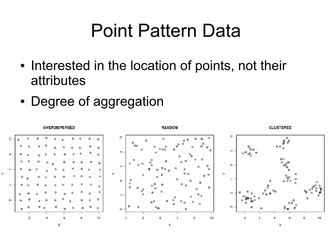
Point Pattern Data

● Interested in the location of points, not their attributes

● Degree of aggregation

Ripley's K

● Calculates counts of points as a function of distance bins for each point

● Combine points together and normalize by area● Positive = more points expected than random

at that distance● Negative = less than expected● Intervals by bootstrap● Requires def'n of area

Ld = A∑i=1

n

∑j=1, j≠1

n

k i , j

n n−1

Ripley's K

Ripley's K in Rlibrary(spatial) ## load library

ppregion(xmin,xmax,ymin,ymax) ## define region

rK <- Kfn(x,max.distance) ## calculate Ripley's K

plot(rK$x,rK$y-rK$x,type='l',xlab="d",ylab="L(d)")##Plot as L(d) rather than K(d)

## compute and plot interval estimateKe <- Kenvl(max.distance, nrep, Psim(n))lines(Ke$x,Ke$upper-Ke$x,lty=2,col="grey")lines(Ke$x,Ke$lower-Ke$x,lty=2,col="grey")

Applications and Extensions

● Irregularly shaped areas● Choice of points counted in each sum can vary

with categorical attribute● Tree maps

– Juvenile aggregated (dispersal)

– Intermediate random (DD mortality)

– Adults are over-dispersed (crown competition)

Point Referenced Data

● Data has a value/attribute plus spatial coordinates but not area

● Aka geospatial data– Origin in mining

● Usually sampling some underlying continuum● Aims:

– Account for lack of independence in data due to spatial proximity (analogous to time series)

– Predict the value at some new location (usually a grid / map)

Examples of Point Ref Data

● Soils– Moisture, nutrients, pH, texture, etc.

● Atmospheric or Ocean measurement– Surface meteorology (temperature, precip, etc.)

– CO2, pollutant concentration, salinity, etc.

● Plot data were size of plot << size of domain– Biomass/abundance, presence/absence, richness

– Invasive species, disease prevalence, etc.

Geospatial Exploratory Analyses

● Smoothing & Detrending● Autocorrelation● Interpolation

– Linear

– Inverse distance weighed

– Geostatistical (Kriging)

● Many packages in R, will focus on most basic & “built in”

Smoothing / Detrending

● Objective: Like with time-series, most statistical methods assume stationarity

● More complicated in 2D (sparse, irregular)● Polynomial (in R, library(spatial) )

– Fit surface: surf.ls(degree, x, y, z)– Project: trmat(surf.obj, xmin, xmax,

ymin, ymax, n)– Plot: image(tr.obj)

Degree 0 Degree 1 Degree 2

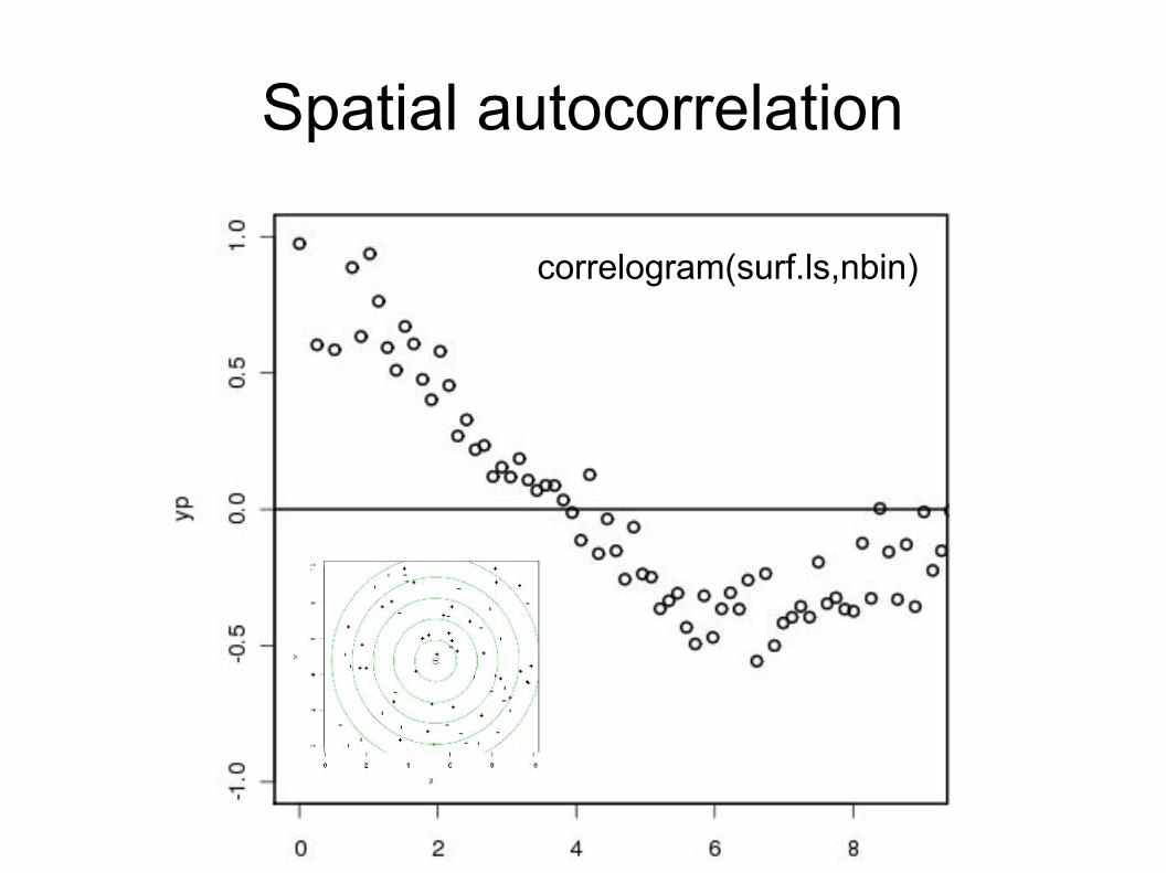
Spatial autocorrelation

correlogram(surf.ls,nbin)

NULL model interval estimate by non-parametric bootstrap

Variogram

● Traditionally, autocorrelation in geostatistics has been expressed in terms of a variogram or semivariogram

● Units = variance d = 1N d ∑

i , j d

N d

Z i−Z j2

● Sill = asymptote● Range = distance

to asymptote● Nugget = variance

at lag 0

variogram(surf.ls,nbin)

Spatial Covariance

● If C(d) is the spatial covariance

● Autocorrelation :

● Variogram :

C d =COV [Z x , Z xd ]

d =C d /C 0

d =C 0−C d

Interpolation

● Objective: predict Z at some new point(s)– Often on a grid to make a raster map

● Linear– Simplest if data already on a grid (four corners)

Interpolation

● Bicubic interpolation: cubic analog to bilinear● Nearest-Neighbor:

– Tesselation

– Voronoi Diagram

● Triangular irregularnetwork (TIN)

Inverse-Distance Weighted

● Previous methods only used nearest points● All are special cases of a weighted average● For irregular, often want to use n-nearest points

or a fixed search radius (variable number of points)

● Requires a way of WEIGHTING points as a function of distance

● Inverse-distance weighted: Wij = 1/d

ij

● Zi = S W

ij Z

j / S W

ij

Spatial Weighted Averages

● Other alternatives to 1/d (e.g. 1/d2)● Major criticisms

– Choice of weighting function somewhat arbitrary, not connected to properties of the data

– Does not account for error in interpolation● Points further from known points should be more

uncertain

● Interpolation vs smoothing– Interpolation always passes exactly though the data

points (0 residuals)

– Smoothing separates trends + residuals

Kriging

● Interpolation based on autocorrelation fcn● Requires fitting an autocorrelation model to the

variogram or correlogram– Provides “weight” to points based on observed

relationship between distance and correlation

– Requires choice of parametric function

● Provides mechanism for estimating interpolation error

Variogram Models

DAIC0.020.55.2

##correlogramcg <- correlogram(data,nbin)

##fit covariance functionexpfit <- function(parm){

-sum(dnorm(cg$y,expcov(cg$x,parm[1]),parm[2],log=TRUE))

}efit <- optim(ic,expfit)

Built in function for exponential covariance

∏ N y∣f x∣ ,2

−∑ log N y∣f x∣ ,2

Step 1: Fit variance model

##detrend accounting for covariancekr <- surf.gls(degree,expcov,data,d=efit$par[1],...)

## matrix prediction (Kriging)pr <- prmat(kr, xmin, xmax, ymin, ymax, n)image(pr)

## matrix errorse <- semat(kr, xmin, xmax, ymin, ymax, n)contour(se3,add=TRUE)

Step 2: Krige surface

Anisotropy● In addition to STATIONARITY (spatial

covariance is the same at all locations), spatial models also assume ISOTROPY, that the spatial covariance is the same in all DIRECTIONS

● Calculate/fit variogram separately for different directions (angular bins) to account for anisotropy– Increases # of parameters, less data points as bins

get smaller

– Alt: modify cov fcn to account for direction

– Alt: fit cov fcn to different subdomains (location)

Flavors of Kriging

● Simple Kriging: mean = 0

● Ordinary Kriging: mean = unknown m● Universial Kriging: mean = polynomial trend● Cokriging: inclusion of covariates

Limitations of Kriging

● Assumes the variogram model is known– Dropped parameter error

● Fitting of variogram model:– Not done as part of overall model fit

– Not done on data directly● Binned means of all n2 pairwise differences

● Detrending and autocorr done separately● Sometimes just want non-independence● Similar to T.S., OK for EDA but ultimately want

to fit whole model at once.