Some Thoughts on Analyzing Topographic Habitat Characteristics Jeff Jenness jeffj@jennessent.com Jenness Enterprises http://www.jennessent.com 3020 N. Schevene Blvd. (928) 607-4638 Flagstaff, AZ 86004 USA

Last Modified February 12, 2007

INTRODUCTION............................................................................................................................... 2 SURFACE AREA............................................................................................................................... 2

SURFACE AREA FROM TINS............................................................................................................ 3 SURFACE AREA FROM GRIDS.......................................................................................................... 3

TOPOGRAPHIC ROUGHNESS .......................................................................................................... 4 SLOPE.............................................................................................................................................. 4

DIRECTIONAL SLOPE ...................................................................................................................... 5 GRAPHICALLY REPRESENTING SLOPE ............................................................................................. 6

ASPECT............................................................................................................................................ 6 GRAPHICALLY REPRESENTING ASPECT ........................................................................................... 7 CLASSIFICATION OF ASPECT VALUES .............................................................................................. 8 DEVIATIONS FROM A BEARING......................................................................................................... 8 SINE AND COSINE TRANSFORMATIONS ............................................................................................ 8 SOLAR INSOLATION: AN ALTERNATIVE TO ASPECT........................................................................... 9

ESRI’s Solar Radiation Tool.................................................................................................................... 9 Hillshades ..............................................................................................................................................10 Solar Analyst..........................................................................................................................................11

LANDSCAPE CURVATURE ............................................................................................................ 11 PROFILE CURVATURE ................................................................................................................... 12 PLANIFORM CURVATURE............................................................................................................... 12 GENERAL CURVATURE ................................................................................................................. 13 PROTECTION................................................................................................................................ 13 TOPOGRAPHIC POSITION INDEX .................................................................................................... 14

Scales and Neighborhoods: ...................................................................................................................15 Neighborhood Options: ..........................................................................................................................17 Classifying by Slope Position: ................................................................................................................18 Classifying by Landform Category: ........................................................................................................20

IN CONCLUSION............................................................................................................................ 24 REFERENCES ................................................................................................................................ 24

2

Introduction I consider terrain analysis to be one of the more interesting and engaging types of geographic analysis. Not only do morphological characteristics of the landscape form critical components of wildlife habitats, but they can be fascinating in their own right. Possibly it’s just me, but I can lose myself staring at a model of a complex landscape in the same way I drift off staring at a campfire.

I have studied and attempted various types of terrain analyses throughout my dual careers as a wildlife biologist with the U.S. Forest Service and as a GIS consultant. Here I lay out some thoughts, and answers to questions I had as I tried different ideas. I hope you find it useful and I would welcome hearing back from readers with different ideas and methods.

Surface Area Wildlife researchers often report area values for some region of interest, such as home range size or number of hectares of a particular habitat type. However, these area values are almost always presented in terms of planimetric area, as if a square kilometer in the Himalayas represents the same amount of landscape surface area as a square kilometer in the Nebraska. Predicted home ranges for wildlife species generally use planimetric area even when describing mountain-dwelling species such as mountain goats (Oreamnos americanus) and puma (Felis concolor). But if a species’ behavior and population dynamics are a function of available resources, and if those resources are spatially limited, then these resources might be better assessed using the surface area of the landscape rather than the planimetric area.

Furthermore, if you consider the amount or proportion of steeply-sloped landscape in an area to be an important habitat component, then consider that the amount or proportion will automatically be underestimated if you derive that value from a planimetric map. The steeper the slope, the more landscape surface area will be compressed into a polygon on a planimetric map.

Digital representations of topography are referred to as Digital Elevation Models (DEMs) and can be defined in vector format as Triangulated Irregular Networks (TINs), or in raster format as an array of pixels with elevation values. Raster datasets are referred to as Grids in ESRI software, and I will refer to raster datasets as Grids for the rest of this discussion. For those who wish to learn more about DEMs, their derivations and their uses, please refer to David Maune’s “Digital Elevation Model Technologies and Applications: The DEM User’s Manual” (Maune 2001).

Calculating surface area can be simple or complicated depending on the data format of your landscape topographic surface. TINs provide more precise estimates of surface area than grids, especially when you have a precisely defined area of interest, and they have the potential to provide more accurate estimates as well, but there are some issues to be aware of. Refer to Jenness (2004) for an in-depth discussion of these issues, but in short they are:

1) TINs are often generated according to a specified accuracy tolerance in which the surface must come within a specific vertical distance of each elevation point, meaning that a TIN surface rarely goes exactly through all the base elevation points on the landscape. This also means that 2 TINs may have been generated with different tolerances, and therefore surface statistics derived from those TINs may not be comparable. This is especially problematic when the TINs are derived using whatever default accuracy is suggested by the software, which generally varies from analysis to analysis based on the range of elevation values in the DEM.

2) Grid computations usually go much faster than TIN computations.

3) Grids lend themselves to neighborhood analyses whereas TINs do not. For example, if you wish to create a dataset in which the value at any point is equal to the minimum, maximum or mean value within a local neighborhood around that point, then you can create this dataset easily with grids.

3

Surface Area from TINs Surface area can be easily calculated from TINs, simply by adding up the areas of all the triangles within an area. ESRI software (3D Analyst in both ArcView 3.x and ArcGIS) provide functions to do this fairly easily. I also have an ArcView 3.x extension that makes it even simpler and includes a few other functions (see my “Surface Tools” extension at http://www.jennessent.com/arcview/surface_tools.htm; Jenness 2005a).

Surface Area from Grids I am aware of 2 reasonable methods for calculating surface area from grids. Joseph Berry describes a way to estimate it based on the slope and cell size of grid cells (Berry 2002). Berry’s method is quick, easy and intuitive.

Berry’s method can be thought of as simply using the slope to calculate an adjustment factor for the cell planimetric area. If the slope is flat, then the adjustment factor is equal to 1 and therefore the surface area is equal to the planimatric area. As the slope increases, the adjustment factor is equal to:

[ ]

1Adjustment Factor(Slope)

where Slope is in , calculated as: Slope (Degrees)

Slope (Radians)180

CosRadians

π

=

=

Therefore, assuming cell size is defined as the length along one edge of the cell, and Slope is measured in degrees, then surface area can be calculated as:

2

Surface Area

180where:

Cell SizeSlope in Degrees

c

Cos S

cS

π=

⎛ ⎞⎛ ⎞⎜ ⎟⎜ ⎟

⎝ ⎠⎝ ⎠

==

One important factor to note about this method is that, because the cell size is constant for all cells, the final surface area grid is perfectly correlated with the Slope grid. Therefore you wouldn’t want to include both Slope and Surface Area in the same statistical model.

There is a potential issue about using this simple method to calculate surface area. Hodgson (1995) describes how most slope and aspect algorithms generate values reflecting an area 1.6 to 2 times the size of the actual cell, which implies that operations that rely on both cell size and slope or aspect may be unduly influenced by adjacent cells. This phenomenon may also lead to artificially high autocorrelation among adjacent slope and aspect cells, although I am not sure what the biological implications of that would be.

I developed another approach, based on partitioning the area of a cell into 8 triangles and calculating the total area of those triangles. This is mathematically more complicated than Berry’s approach, but I have written an ArcView 3.x extension to simplify it (see my “Grid Surface Areas” extension at http://www.jennessent.com/arcview/surface_areas.htm; Jenness 2002).

The methods, plus an analysis of the accuracy and precision of the results, are described in detail in Jenness (2004) and in the manual for the “Grid Surface Areas” extension. A high-resolution poster illustrating the steps is also available to download (see http://www.jennessent.com/arcview/surf_area_poster.htm).

4

Topographic Roughness Terrain irregularity can be defined in a number of ways. Hobson (1972:221-245) discussed the concept of dividing the surface area by the planimetric area to get a surface area ratio. Bowden et al. (2003) found that ratio estimators of Mexican spotted owl (Strix occidentalis lucida) population size were more precise using a version of this surface area ratio than with planimetric area. I have personally found the surface area ratio value to be useful in analyzing topographic characteristics of Mexican spotted owl habitat, and both my Grid Surface Areas extension (Jenness 2002) and my Surface Tools extension (Jenness 2005a) offer options to calculate the surface area ratio of a landscape.

Beasom (1983) described a method for estimating land surface ruggedness based on the intersections of sample points and contour lines on a contour map, and Jenness (2000) and Jenness et al. (2004) described a similar method based on measuring the density of contour lines in an area. Mandelbrot (1983:29, 112-115) described the concept of a “fractal dimension” in which the dimension of an irregular surface lies between 2 (representing a flat plain) and 3 (representing a surface that goes through every point within a volume). Calculating this fractal dimension can be very challenging computationally, and Polidori et al. (1991), Lam & De Cola (1993:30-38) and Lorimer et al. (1994:9-10) discussed a variety of methods for estimating the fractal dimension for a landscape. Rugosity is a special type of roughness measure describing how wrinkled a surface is.

Slope Slope is an important habitat characteristic for many species, and is generally defined as the absolute value of the slope in the steepest direction. Several algorithms are available to calculate the slope of a cell based on some combination of the elevation value in that cell and the 8 adjacent cells. In an early example, given a simple elevation grid with 9 cells labeled A – I:

Figure 1: Sample elevation grid with 9 cells, where each cell has an elevation value associated with it. There are a variety of methods available to calculate the slope of the focal (central) cell based on the elevation values in the neighboring cells.

Evans (1972) defines slope (or gradient) as the 1st derivative of the landscape surface, calculated as:

5

( ) ( )2 2

1 1 1 1

1

1

1

1

2, , , ,

,

,

,

,

Gradient (Evans 1972, p. 52)

where Cell BCell H

Cell DCell F

Cell Size

i j i j i j i j

i j

i j

i j

i j

Z Z Z Z

dZ

Z

Z

Z

d

+ − − +

+

−

−

+

− + −=

=

=

=

=

=

In this text, Evans also discusses several other terrain measures originally developed by W. R. Tobler.

ESRI software uses the slope algorithm described by Burrough & McDonnell (1998, p. 190-193; see also http://support.esri.com/index.cfm?fa=knowledgebase.techarticles.articleShow&d=21345), where:

( ) ( )( )

( ) ( )( )

2 2

2

2

2 28

2 28

% Slope

where cell size

where cell size

x y

x

y

Z Z

A D G C F IZ

A B C G H IZ

Δ Δ

Δ

Δ

= +

+ + − + +=

+ + − + +=

In general:

( )180Slope in Degrees Arctan % Slopeπ

=

Kevin Jones provides an excellent discussion and comparison of 8 slope algorithms (Jones 1998), ranking them in order of accuracy when applied to two complex surfaces in which the true slopes are known. The ESRI algorithm, described as Horn’s method in Jones’ paper, ranked 2nd in accuracy on one surface and 3rd on another surface.

Directional Slope You may have an interest in calculating the slope in a particular direction. There are no ESRI functions to do this directly, but I have a free ArcView 3.x extension that will calculate these data if you ever have the need for them (see “Directional Slopes” at http://www.jennessent.com/arcview/dir_slopes.htm; Jenness 2005b). The logic involved is reasonably straightforward. The directional slope value for a cell is based on the slope from that cell center to an interpolated point lying somewhere on a ring connecting the cell centers of the 8 adjacent cells. For example, if you were interested in calculating the slopes at 247.5 degrees, the extension would interpolate a point between the cell centers of the southwestern and western cells and calculate the slope to that point.

6

Figure 2: Slope in a particular direction is derived by interpolating an elevation value at a point between 2 adjacent cells, and calculating the slope from the focal cell center to that interpolated point.

Graphically Representing Slope Slope can easily be represented graphically, using a diagram that simply shows a line angled at the same angle as the average slope. Such a graphic is very easy and intuitive to understand.

I prefer a modification of this, showing the range and standard deviation along with the mean. This image clearly conveys the variation of the data along with the mean:

Both of these options are available in the free “Grid Tools” ArcView 3.x extension (Jenness 2006).

Aspect Aspect is an intuitively valuable habitat variable. North-facing slopes are typically cooler and more mesic while south-facing slopes are generally warmer and more xeric (at least in the northern hemisphere!), and habitats can be dramatically different depending on which side of a hill you stand on. Aspect can be difficult to analyze, though, because of its circular nature. The difference between 1 degree and 360 degrees is the same as the difference between 1 degree and 2 degrees, making it difficult to plug into a typical statistical model.

7

Fortunately there are well-established methods available for analyzing circular or periodic data such as aspect values. The circular nature of the data lead to very specific and interesting approaches to calculating measures of central tendency and dispersion. Some of the basic statistics are:

( )( )( )

( )

2 2 2

1 1

1

1

1

2

0 0

0

2 0 0

1

2 1

Where: cos sin

tan ,

Mean Direction: tan

tan ,

Circular Variance: V (Mardia & Jupp, Fisher)

Angular Variance: (Batschelet)

Circu

n n

i ii i

RC S R C S Rn

S C S C

S C C

S C S C

R

s R

θ θ

θ π

π

= =

−

−

−

= = = + =

⎧ > >⎪⎪= + <⎨⎪

+ < >⎪⎩= −

= −

∑ ∑

( ) ( )

( ) ( )

( )

2

2

2 1

180

lar Standard Deviation: ln In Radians (Mardia & Jupp, Fisher)

Angular Deviation: In Radians (Batschelet)

Radians to Degrees:

v R

s s R

Degrees Radiansπ

= −

= = −

=

Please refer to Mardia & Jupp (2000), Zar (1999; see especially ch. 26 and 27), Fisher (1993) and Batschelet (1981) for some good texts on circular statistics, distributions (i.e. the Fisher, Von Mises and Wrapped Normal distributions), and circular hypothesis testing.

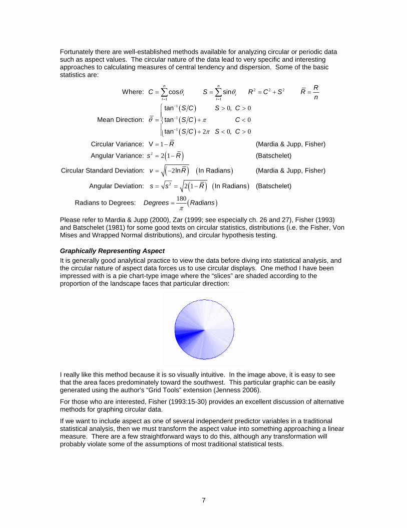
Graphically Representing Aspect It is generally good analytical practice to view the data before diving into statistical analysis, and the circular nature of aspect data forces us to use circular displays. One method I have been impressed with is a pie chart-type image where the “slices” are shaded according to the proportion of the landscape faces that particular direction:

I really like this method because it is so visually intuitive. In the image above, it is easy to see that the area faces predominately toward the southwest. This particular graphic can be easily generated using the author’s “Grid Tools” extension (Jenness 2006).

For those who are interested, Fisher (1993:15-30) provides an excellent discussion of alternative methods for graphing circular data.

If we want to include aspect as one of several independent predictor variables in a traditional statistical analysis, then we must transform the aspect value into something approaching a linear measure. There are a few straightforward ways to do this, although any transformation will probably violate some of the assumptions of most traditional statistical tests.

8

Classification of Aspect Values Probably the easiest transformation is to simply group your aspect values into general direction ranges (for example, “N” = 315 – 45, “E” = 45 – 135, “S” = 135 – 225, and “W” = 225 - 315), creating a categorical dataset which may be appropriate for some analyses.

Deviations from a Bearing A simple and basic transformation is to convert your aspect values into deviations from a direction of interest. For example, if you felt that the object of your study was likely to be affected by the north- vs. south-facing slope phenomenon, then you might define your aspect values in terms of “Deviations from North” where each aspect value would reflect the distance, in degrees, from due North. Your full set of transformed values would range from 0 to 180 (see Figure 3). This option has the advantage of maintaining a constant interval between units, such that the difference in direction between 0 and 1 degree is the same as the difference between 90 and 91 degrees.

Sine and Cosine Transformations Aspect values are often converted to sine and cosine values, essentially decomposing them into north-south and east-west components. Sine values range from -1 (at due west) to 1 (at due east), while cosine values range from -1 (at due south) to 1 (at due north) (see Figure 3). Note that this method does not maintain a constant interval between units. The sine and cosine values change by a variable amount depending on the direction, such that a change in sine corresponding to a change of 1 degree = 0.00015 when going from 90 to 91 degrees, but increases by more than 2 orders of magnitude to 0.017 when going from 180 to 181 degrees. This issue may be important in your statistical analysis if your method assumes that your data are interval-level.

Figure 3: Transformations of Aspect Values

9

Trimble & Weitzman (1956) and Beers et al. (1966) suggest an interesting alternative combining two of the approaches above, rescaling aspect values based on an optimum bearing (45 degrees in their example) and then taking the sine of the rescaled values, which they put to extensive use in site productivity research for timber stands.

Solar Insolation: An alternative to Aspect Aspect has a well-established history in habitat analysis. It is both easy to measure and a good predictor of certain habitat characteristics. However, in some cases we are really interested in how much direct sunlight hits an area (insolation), which is a function of aspect, slope, nearby topography, landscape reflectivity and atmospheric effects, and which may be a more important driver of habitat characteristics than aspect alone. In such cases, it may be worthwhile to estimate insolation directly rather than use aspect as a surrogate. There are a few approaches you can take:

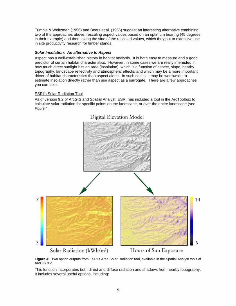
ESRI’s Solar Radiation Tool As of version 9.2 of ArcGIS and Spatial Analyst, ESRI has included a tool in the ArcToolbox to calculate solar radiation for specific points on the landscape, or over the entire landscape (see Figure 4.

Figure 4: Two option outputs from ESRI’s Area Solar Radiation tool, available in the Spatial Analyst tools of ArcGIS 9.2.

This function incorporates both direct and diffuse radiation and shadows from nearby topography. It includes several useful options, including:

10

1) Outputs either the amount of energy hitting the ground, in Watts per Hour, or the total number of hours in which the ground is exposed to the sun.

2) Can be calculated for specific dates, seasons or years.

3) Has optional parameters where you can specify the general atmospheric conditions in your area of interest.

4) Has optional parameters where you can specify how intensively it examines the local topography before determining the amount of radiation hitting an area.

In general, this is a wonderful and exciting new tool. I have noticed two minor drawbacks to the tool:

1) It is slow on large grids, and on occasion I have needed to let it run for hours or days.

2) I do not believe that it incorporates reflectivity off the landscape. This would be hard to model, of course, and would depend on exactly how reflective your landscape is (snow reflects very differently from lava rocks, for example).

Despite these two minor drawbacks, I expect that this tool will become very valuable for habitat analysis.

Hillshades If you do not have version 9.2 or greater of ArcGIS and Spatial Analyst, or if you do not have the time to calculate proper solar radiation parameters for your landscape, then hillshades offer a simple and quick alternative.

Any decent GIS system that works with raster data should be able to generate a hillshade from an elevation dataset. These hillshades are typically used to enhance the aesthetic qualities of the elevation grid, or to help you quickly identify where hills and valleys are. ESRI software produces hillshades with grid cell values ranging from 0 to 255 based on how directly the grid cell faces the sun. A value of 0 means that no sunlight is hitting that grid cell (either simply not facing the sun, or shadowed behind another topographic feature) while a value of 255 means the grid cell faces the sunlight directly. The user simply enters an azimuth and angle of elevation for the sun location.

By the way, as an interesting trivial aside, the default ESRI settings for sun location are 315 degrees azimuth and 45 degrees elevation, which are unlikely values for most places in the northern hemisphere. It turns out that using realistic values (such as having the sun come from the south rather than the north) causes an optical illusion for many viewers in which the topography appears to be inverted (i.e. valleys look like hilltops and vice versa).

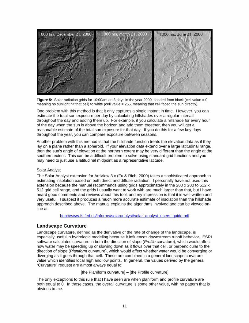
Aesthetic properties aside, the fact that the hillshade tells you how directly the grid cell faces the sun, including whether it is shadowed by other features, makes it a useful estimate of insolation (at least for a single instant in time; see Figure 5). The trick is to determine the correct bearing and angle of elevation for the sun, given your location and a particular instant in time. You can do this by either writing your own spherical geometry functions in your coding language of choice, or use a free tool such as the online Naval Observatory Solar Position Calculator (U.S. Naval Observatory 2005). I personally like this tool because it produces a table of values over a predefined interval throughout the day.

11

Figure 5: Solar radiation grids for 10:00am on 3 days in the year 2000, shaded from black (cell value = 0, meaning no sunlight hit that cell) to white (cell value = 255, meaning that cell faced the sun directly).

One problem with this method is that it only captures a single instant in time. However, you can estimate the total sun exposure per day by calculating hillshades over a regular interval throughout the day and adding them up. For example, if you calculate a hillshade for every hour of the day when the sun is above the horizon and add them together, then you will get a reasonable estimate of the total sun exposure for that day. If you do this for a few key days throughout the year, you can compare exposure between seasons.

Another problem with this method is that the hillshade function treats the elevation data as if they lay on a plane rather than a spheroid. If your elevation data extend over a large latitudinal range, then the sun’s angle of elevation at the northern extent may be very different than the angle at the southern extent. This can be a difficult problem to solve using standard grid functions and you may need to just use a latitudinal midpoint as a representative latitude.

Solar Analyst The Solar Analyst extension for ArcView 3.x (Fu & Rich, 2000) takes a sophisticated approach to estimating insolation based on both direct and diffuse radiation. I personally have not used this extension because the manual recommends using grids approximately in the 200 x 200 to 512 x 512 grid cell range, and the grids I usually want to work with are much larger than that, but I have heard good comments and reviews about this tool, and my impression is that it is well-written and very useful. I suspect it produces a much more accurate estimate of insolation than the hillshade approach described above. The manual explains the algorithms involved and can be viewed on-line at:

http://www.fs.fed.us/informs/solaranalyst/solar_analyst_users_guide.pdf

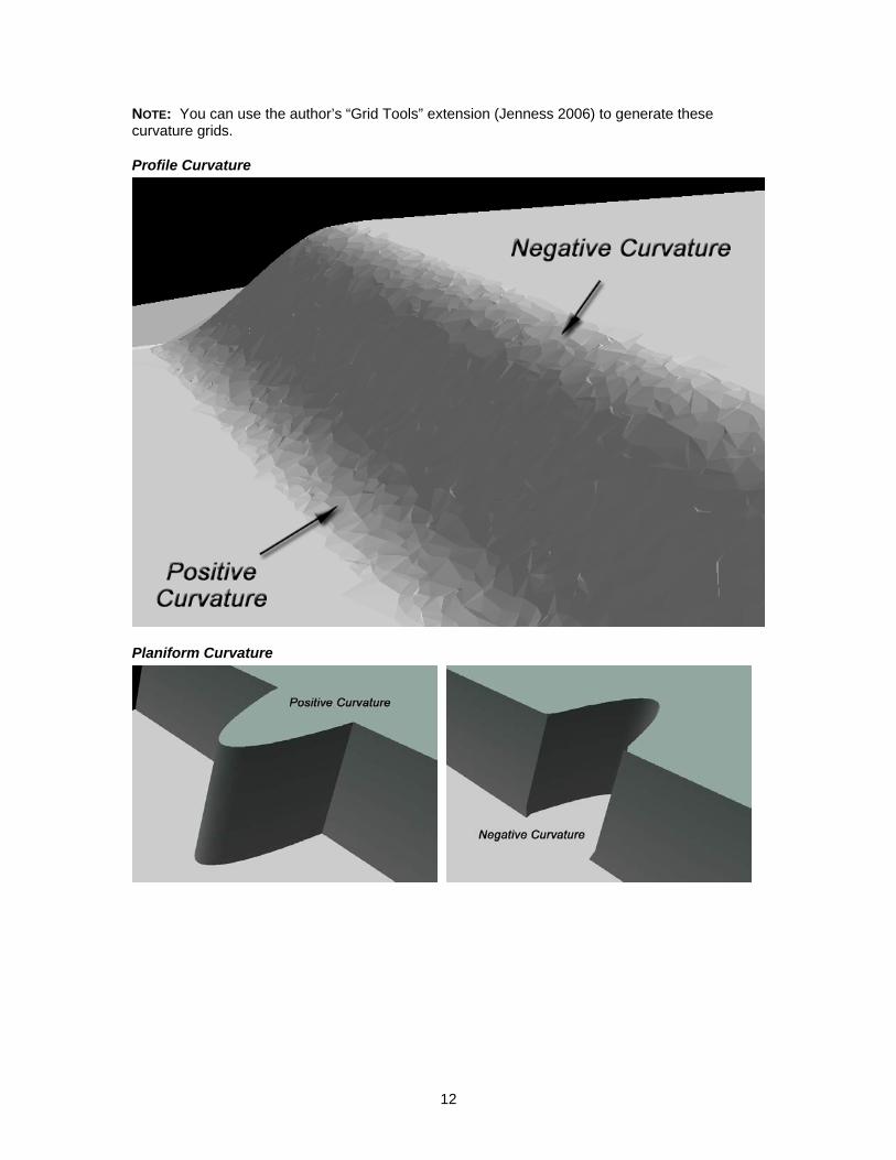
Landscape Curvature Landscape curvature, defined as the derivative of the rate of change of the landscape, is especially useful in hydrologic modeling because it influences downstream runoff behavior. ESRI software calculates curvature in both the direction of slope (Profile curvature), which would affect how water may be speeding up or slowing down as it flows over that cell, or perpendicular to the direction of slope (Planiform curvature), which would affect whether water would be converging or diverging as it goes through that cell. These are combined in a general landscape curvature value which identifies local high and low points. In general, the values derived by the general “Curvature” request are almost always equal to:

[the Planiform curvature] – [the Profile curvature]

The only exceptions to this rule that I have seen are when planiform and profile curvature are both equal to 0. In those cases, the overall curvature is some other value, with no pattern that is obvious to me.

12

NOTE: You can use the author’s “Grid Tools” extension (Jenness 2006) to generate these curvature grids.

Profile Curvature

Planiform Curvature

13

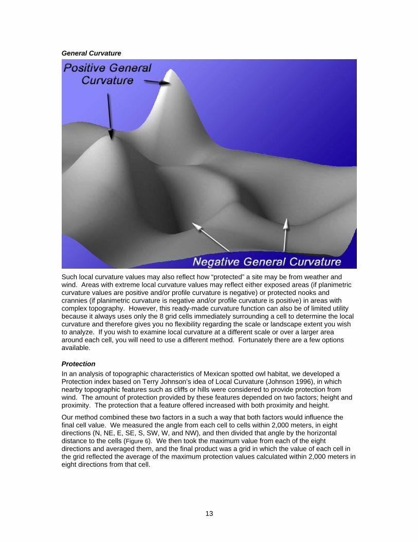
General Curvature

Such local curvature values may also reflect how “protected” a site may be from weather and wind. Areas with extreme local curvature values may reflect either exposed areas (if planimetric curvature values are positive and/or profile curvature is negative) or protected nooks and crannies (if planimetric curvature is negative and/or profile curvature is positive) in areas with complex topography. However, this ready-made curvature function can also be of limited utility because it always uses only the 8 grid cells immediately surrounding a cell to determine the local curvature and therefore gives you no flexibility regarding the scale or landscape extent you wish to analyze. If you wish to examine local curvature at a different scale or over a larger area around each cell, you will need to use a different method. Fortunately there are a few options available.

Protection In an analysis of topographic characteristics of Mexican spotted owl habitat, we developed a Protection index based on Terry Johnson’s idea of Local Curvature (Johnson 1996), in which nearby topographic features such as cliffs or hills were considered to provide protection from wind. The amount of protection provided by these features depended on two factors; height and proximity. The protection that a feature offered increased with both proximity and height.

Our method combined these two factors in a such a way that both factors would influence the final cell value. We measured the angle from each cell to cells within 2,000 meters, in eight directions (N, NE, E, SE, S, SW, W, and NW), and then divided that angle by the horizontal distance to the cells (Figure 6). We then took the maximum value from each of the eight directions and averaged them, and the final product was a grid in which the value of each cell in the grid reflected the average of the maximum protection values calculated within 2,000 meters in eight directions from that cell.

14

Figure 6: Protection depends on both proximity and height. In this case, Point B is both higher and at a steeper angle from the origin than Point A, yet Point A outscores Point B because it is closer. Using this method, we would conclude that a 300-meter cliff located 200 meters away would offer almost twice as much protection as a 750-meter cliff located 400 meters away (with respective scores of 0.280 and 0.155). This calculation is repeated eight times in eight directions, and the final cell value reflects the average of maximum protection values calculated in the eight directions.

It may be debatable as to whether the protection offered by some topographic feature can be quantified this easily, but this method does have the advantage of producing protection values proportional to the height and proximity of a feature (Figure 7). In other words, the protection value of a 100-meter cliff will be twice that of a 50-meter cliff, assuming the cliffs are both the same distance away. Likewise, the protection value of a cliff 50 meters away will be twice that of a cliff 100 meters away, assuming both cliffs are the same height.

Figure 7: Different combinations of height and proximity can produce the same protection values. In this example, a 67-meter cliff 80 meters away offers the same protection value as a 3.6-meter cliff 20 meters away.

Topographic Position Index Andrew Weiss presented a very interesting and useful poster at the 2001 ESRI International User Conference describing the concept of Topographic Position Index (TPI) and how it could be calculated (Weiss 2001; see also Guisan et al. 1999 and Jones et al. 2000). Using this TPI at different scales, plus slope, users can classify the landscape into both slope position (i.e. ridge

15

top, valley bottom, mid-slope, etc.) and landform category (i.e. steep narrow canyons, gentle valleys, plains, open slopes, mesas, etc.).

The algorithms are clever and fairly simple. The TPI is the basis of the classification system and is simply the difference between a cell elevation value and the average elevation of the neighborhood around that cell. Positive values mean the cell is higher than its surroundings while negative values mean it is lower.

The degree to which it is higher or lower, plus the slope of the cell, can be used to classify the cell into slope position. If it is significantly higher than the surrounding neighborhood, then it is likely to be at or near the top of a hill or ridge. Significantly low values suggest the cell is at or near the bottom of a valley. TPI values near zero could mean either a flat area or a mid-slope area, so the cell slope can be used to distinguish the two.

Scales and Neighborhoods: TPI is naturally very scale-dependent. The same point at the crest of a mountain range might be considered a ridgetop to a highway construction crew or a flat plain to a mouse. The classifications produced by this method depend entirely on the scale you use to analyze the landscape.

For example, in the illustration below, TPI is calculated for the same point on the landscape using 3 different scales. In each case, the point is located on top of a small hill set inside a larger valley. In Case A, the scale is small enough that the point is at about the same elevation as the entire analysis region so the TPI value would be approximately 0. In Case B, the analysis region is big enough to encompass the entire small hill, and the point is consequently much higher than its neighbors and has a correspondingly high TPI value. In Case C, the neighborhood includes the hills on either side of the valley, and therefore the point is lower than its neighbors and has a negative TPI value.

Users should consider carefully what scale is most relevant for the phenomenon being analyzed. If you are interested in topographic habitat characteristics of large, wide-ranging animals, you would likely define your landscape classifications in terms of large, distinctive topographic

16

features. Cougars, for example, are likely to be much more influenced by a nearby ridgeline hundreds of feet high than in minor ripples and bumps on the landscape immediately surrounding them. Furthermore, a point on top of a small hill at the bottom of a canyon may be classified as a canyon bottom at one scale, or a hilltop at a different scale. Both are accurate and valid classifications, and the user must be responsible for knowing what scale is reasonable for their analysis.

Scale is determined by the neighborhood used in the analysis. The TPI values reflect the difference between the elevation in a particular cell and the average elevation of the cells around that cell. The Neighborhood defines what cells are considered to be “around” that cell.

In the illustration below, TPI values were calculated using 2 different neighborhoods. The left example used a circular neighborhood with a 500m radius, meaning that the TPI value for each cell reflected the difference between the elevation of that cell and the average elevation of all cells within 500m of that cell. This neighborhood did a good job of identifying extreme values in the side drainages of the canyon. The example on the right used a circular neighborhood with a 2000m radius and did a much better job of highlighting the overall canyon system.

These examples used circular neighborhoods, but other options are available. Weiss’ examples used annular (ring- or doughnut-shaped) neighborhoods where only cells within a specified distance range are considered. Some researchers use rectangular neighborhoods, although in most cases circular or annular neighborhoods are more reasonable.

17

Wedge-shaped neighborhoods are useful for restricting your analysis to a particular direction. Weiss’ poster discusses some ideas for future research in which he plans to compare directional TPI values in order to distinguish saddles from flat areas, ridges from hilltops and valleys from local depressions, as well as identify the general aspect of landforms.

For sophisticated neighborhood delineation, you can also define exactly which local cells should be considered as a neighborhood. These are referred to as “irregular” neighborhoods in ESRI software, and there are a few extensions available that can generate such irregular neighborhoods (see esp. Jenness [2006] and Jenness [2005c]).

Neighborhood Options: When conducting any kind of neighborhood analysis, the size and type of neighborhood is naturally critical to the output. In all cases the cell values in the final output grid will reflect some statistic (minimum, maximum, standard deviation, etc.) of the cell values in the “neighborhood” around each cell. Most neighborhood analysis can be handled with such standard neighborhood shapes as circles, rings, wedges and rectangles. In some cases you may wish to construct a specific irregular neighborhood shape, which is generally not possible through the basic GIS interface but which is possible with some free ArcView extensions (see esp. Jenness [2006] and Jenness [2005c]).

a) Circle: A circular neighborhood defined by a radius length extending outward from the cell center. In theory, this neighborhood should be composed of all grid cells whose cell centers lie within that distance of the focal cell center, but Spatial Analyst appears to have some kind of number rounding issue that sometimes includes or excludes cells that do not exactly fit this definition. If possible, test the neighborhood function to make sure it is including the all the cells you need it to. If not, you may be able to use Custom Neighborhood functions to create a correct neighborhood.

b) Annulus: An annular neighborhood looks like a ring or doughnut defined by an inner and outer radius length extending outward from the cell center. This neighborhood should be composed of all cells whose cell centers lie within this ring, but this can also be affected by the rounding issues that affect the Circular neighborhood. If testing reveals that the annular neighborhood is not working exactly as desired, you may be able to generate a custom neighborhood that will work correctly.

c) Wedge: A wedge-shaped neighborhood looks like a slice of pie cut out of a circular neighborhood and is defined by a starting angle, and ending angle, and a radius. As always, it is advisable to test and confirm that your neighborhood is correct, and possibly generate a custom neighborhood if necessary.

18

d) Rectangle: A square or rectangular neighborhood defined by width and height, which will be centered around your focal cell center. Cells will be included in the neighborhood if the cell centers lie within this rectangle.

e) Irregular: Irregular neighborhoods can be of any shape or arrangement and are defined by explicitly stating which cells, relative to the focal cell, will be included in the neighborhood. This type of neighborhood is generally not available through the standard GIS interface, but can be created using 3rd-party add-on extensions such as Jenness (2006) and Jenness (2005c).

Classifying by Slope Position: TPI values can easily be classified into slope position classes based on how extreme they are and by the slope at each point. There are a couple of strategies you can take to do this.

The easiest way is simply to set threshold values for the TPI grids themselves (or for standardized TPI grids, in which all TPI values are rescaled to a mean of 0 and a standard deviation of 1; see http://www.jennessent.com/arcview/tpi.htm for examples). TPI values above a certain threshold might be classified as ridgetops or hilltops while TPI values below a threshold might be classified as valley bottoms or depressions. TPI values near 0 could be classified as flat plains (if the slope is near 0) or as mid-slope areas (if the slope is above a certain threshold). Dickson and Beier (in review) use this method in a study of the influences of topography on cougar movement.

A somewhat more sophisticated method, illustrated by Weiss in his poster, is to define threshold TPI values in terms of standard deviations from the elevation, which therefore take into account the variability of elevation values within that neighborhood. This means that grid cells with identical TPI value may be classified differently in different areas, depending on the variability in their respective neighborhoods. This method may or may not be useful in your analysis. You would use this method if you felt that cells with high neighborhood elevation variability should have to meet a higher TPI threshold in order to be classified into some category.

As with TPI values in general, neighborhood size is also a critical component of the Slope Position classification process. Small neighborhoods capture small and local hills and valleys while large neighborhoods capture larger-scale features.

19

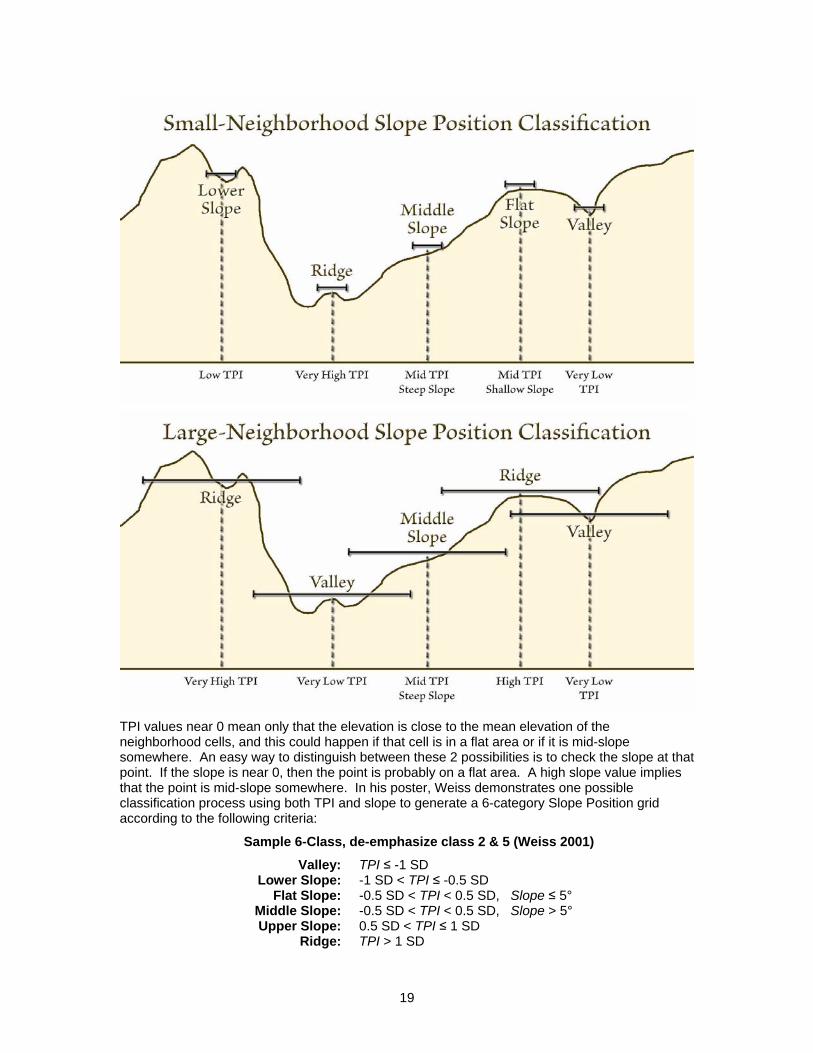
TPI values near 0 mean only that the elevation is close to the mean elevation of the neighborhood cells, and this could happen if that cell is in a flat area or if it is mid-slope somewhere. An easy way to distinguish between these 2 possibilities is to check the slope at that point. If the slope is near 0, then the point is probably on a flat area. A high slope value implies that the point is mid-slope somewhere. In his poster, Weiss demonstrates one possible classification process using both TPI and slope to generate a 6-category Slope Position grid according to the following criteria:

Sample 6-Class, de-emphasize class 2 & 5 (Weiss 2001)

Valley: TPI ≤ -1 SD Lower Slope: -1 SD < TPI ≤ -0.5 SD Flat Slope: -0.5 SD < TPI < 0.5 SD, Slope ≤ 5° Middle Slope: -0.5 SD < TPI < 0.5 SD, Slope > 5° Upper Slope: 0.5 SD < TPI ≤ 1 SD Ridge: TPI > 1 SD

20

Classifying by Landform Category: Landform category can be determined by classifying the landscape using 2 TPI grids at different scales. The combination of TPI values from different scales suggest various landform types.

21

For example, a high TPI value in a small neighborhood, combined with a low TPI value in a large neighborhood, would be classified as a local ridge or hill in a larger valley, while a low small-neighborhood TPI plus a high large-neighborhood TPI would be classified as an upland drainage or depression.

22

Weiss’ poster provides examples demonstrating how 2 TPI grids and a slope grid can be used to identify canyons, mid-slope drainages, U-shaped valleys, plains, open slopes, upper slopes, mesas, mid-slope ridges and mountain tops, according to the following classification criteria:

Sample 10-Class, Landform Classification (Weiss 2001; slightly modified)

Canyons, Deeply Incised Streams: Small Neighborhood TPI: TPI ≤ -1 Large Neighborhood TPI: TPI ≤ -1 Midslope Drainages, Shallow Valleys: Small Neighborhood TPI: TPI ≤ -1 Large Neighborhood TPI: -1 < TPI < 1 Upland Drainages, Headwaters: Small Neighborhood TPI: TPI ≤ -1 Large Neighborhood TPI: TPI ≥ 1 U-shaped Valleys: Small Neighborhood TPI: -1 < TPI < 1 Large Neighborhood TPI: TPI ≤ -1 Plains Small: Neighborhood TPI: -1 < TPI < 1 Large Neighborhood TPI: -1 < TPI < 1 Slope ≤ 5° Open Slopes: Small Neighborhood TPI: -1 < TPI < 1 Large Neighborhood TPI: -1 < TPI < 1 Slope > 5° Upper Slopes, Mesas: Small Neighborhood TPI: -1 < TPI < 1 Large Neighborhood TPI: TPI ≥ 1 Local Ridges/Hills in Valleys: Small Neighborhood TPI: TPI ≥ 1 Large Neighborhood TPI: TPI ≤ -1 Midslope Ridges, Small Hills in Plains: Small Neighborhood TPI: TPI ≥ 1 Large Neighborhood TPI: -1 < TPI < 1 Mountain Tops, High Ridges: Small Neighborhood TPI: TPI ≥ 1 Large Neighborhood TPI: TPI ≥ 1

23

I have a free ArcView 3.x extension that simplifies calculating TPI using Weiss’ algorithms, and includes ways to save and share classification criteria sets. If you would like to use the extension, or just review the manual for a more in-depth discussion of the algorithms involved, please my TPI page at http://www.jennessent.com/arcview/tpi.htm.

24

In Conclusion Digital elevation models offer many more potential habitat descriptors than simply a set of elevation values. With a bit of creativity and imagination, DEMs can yield a wide variety of landscape morphological characteristics which may be important to wildlife, land managers and researchers. Elevation data are becoming more and more available (see especially the National Elevation Dataset (NED; see Gesch et al. 2002) and the 2000 Shuttle Radar Topography Mission (SRTM; Jet Propulsion Laboratories 2000), both of which are available at the USGS Seamless Data Distribution site; see http://seamless.usgs.gov/; USGS 2005)

This article describes some of the analytical approaches and topographic concepts I have encountered over the years. I would enjoy hearing back from people regarding terrain analytical methods that have worked for you. You can reach me at jeffj@jennessent.com.

References Batschelet, E. 1981. Circular Statistics in Biology. Academic Press.

Beasom, S. L. 1983. A technique for assessing land surface ruggedness. Journal of Wildlife Management. 47: 1163–1166.

Beers, T. W., P. E. Dress, and L. C. Wensel. 1966. Aspect transformation in site productivity research. Journal of Forestry 64:691-692.

Berry, J. K. 2002. Use surface area for realistic calculations. Geoworld 15(12): 20–1. Available at http://www.geoplace.com/gw/2002/0212%5Fgw/0212bmp.asp

Bowden, D. C., G. C. White, A. B. Franklin, and J. L. Ganey. 2003. Estimating population size with correlated sampling unit estimates. Journal of Wildlife Management 67: 1–10

Burrough, P. A. and R. McDonnell. 1998. Principals of Geographical Information Systems. Oxford University Press.

Dickson, B. and P. Beier. In Review. Influence Of Topographic Position On Cougar Movement In Southern California.

Evans, I. S. 1972. Chapter 2 – General geomorphometry, derivations of altitude and descriptive statistics. Pages 17-90 in R. J. Chorley, Editor. Spatial analysis in geomorphology. Harper & Row, Publishers. New York, New York, USA.

Fisher, N. I. 1993. Statistical Analysis of Circular Data. Cambridge University Press.

Fu, P. and P. M. Rich. 2000. The solar analyst 1.0. Helios Environmental Modeling Institute, LLC. Available at http://www.fs.fed.us/informs/download.php. Accessed on May 6, 2005.

Gesch, D., M. Oimoen, S. Greenlee, C. Nelson, M. Steuck, and D. Tyler. 2002. The national elevation dataset. Photogrammetric Engineering & Remote Sensing 68:5-11.

Guisan, A., S. B. Weiss and A. D. Weiss. 1999. GLM versus CCA spatial modeling of plant species distribution. Kluwer Academic Publishers. Plant Ecology. 143:107-122.

Hobson, R. D. 1972. Chapter 8 - surface roughness in topography: quantitative approach. Pages 221-245 in R. J. Chorley, editor. Spatial analysis in geomorphology. Harper & Row, New York, New York, USA.

Hodgson, M. E. 1995. What cell size does the computed slope/aspect angle represent? Photogrammetric Engineering & Remote Sensing 61: 513-517.

Jenness, J. S. 2000. The effects of fire on Mexican spotted owls in Arizona and New Mexico. Thesis, Northern Arizona University, Flagstaff, Arizona, USA. Available at: http://www.jennessent.com/downloads/owls_fire_thesis_jenness.pdf

Jenness, J. S. 2002. Surface Areas and Ratios from Elevation Grid (surfgrids.avx) extension for ArcView 3.x, v. 1.2. Jenness Enterprises. Available at: http://www.jennessent.com/arcview/surface_areas.htm.

25

Jenness, J. S. 2004. Calculating landscape surface area from digital elevation models. Wildlife Society Bulletin. 32(3):829-839. Available at http://www.rmrs.nau.edu/publications/rmrs_2004_jennessj001.pdf

Jenness, J. S. 2006. Grid Tools (Jenness Enterprises) v. 1.5 (grid_tools_jen.avx) extension for ArcView 3.x. Jenness Enterprises. Available at: http://www.jennessent.com/arcview/grid_tools.htm.

Jenness, J. S., P. Beier and J. L. Ganey. 2004. Associations between forest fire and Mexican spotted owls. Forest Science 50(6). p. 765 – 772. Available at: http://www.jennessent.com/downloads/owls_and_fire_jenness_et_al.pdf

Jenness, J. S. 2005a. Surface Tools (surf_tools.avx) extension for ArcView 3.x, v. 1.6. Jenness Enterprises. Available at: http://www.jennessent.com/arcview/surface_tools.htm.

Jenness, J. S. 2005b. Directional Slope (dir_slope.avx) extension for ArcView 3.x. Jenness Enterprises. Available at: http://www.jennessent.com/arcview/dir_slopes.htm.

Jenness, J. S. 2005c. Topographic Position Index (tpi_jen.avx) extension for ArcView 3.x. Jenness Enterprises. Available at: http://www.jennessent.com/arcview/tpi.htm.

Jet Propulsion Laboratory. 2000. Shuttle Radar Topography Mission (Web Page). Located at: http://www.jpl.nasa.gov/srtm/. Accessed on May 12, 2005.

Johnson, Terrell H. 1996. Topographic model of potential spotted owl habitat in northern New Mexico. Santa Fe National Forest PO 43-8379-5-0391. Los Alamos National Laboratory Agreement C-5379. P.O. Box 327, Los Alamos, NM 87544. 10 pp.

Jones , K.B., D.T. Heggem, T.G. Wade, A.C. Neale, D.W. Ebert, M.S. Nash, M.H. Mehaffey, K.A. Hermann, A.R. Selle, S. Augustine, I.A. Goodman, J. Pedersen, D. Bolgrien, J.M. Viger, D. Chiang, C.J. Lin, Y. Zhong, J. Baker And R.D. Van Remortel. 2000. Assessing Landscape Conditions Relative to Water Resources in the Western United States: A Strategic Approach. Environmental Monitoring and Assessment 64: 227 – 245.

Jones, K. H. 1998. A comparison of two approaches to ranking algorithms used to compute hill slopes. GeoInformatica 1:3, 235-256. Kluwer Academic Publishers, Boston.

Lam, N. S. N., and L. DeCola. 1993. Fractals in Geography. PTR Prentice-Hall, Englewood Cliffs, New Jersey, USA.

Lorimer, N. D., R. G. Haight, and R. A. Leary. 1994. The fractal forest: fractal geometry and applications in forest science. United States Department of Agriculture Forest Service, North Central Forest Experiment Station, General Technical Report; NC-170. St. Paul, Minnesota, USA.

Mandelbrot, B. B. 1983. The fractal geometry of nature. W. H. Freeman and Company, New York, New York, USA.

Mardia, K. V. and P. E. Jupp. Directional Statistics. Wiley Series in Probability and Statistics. John Wiley and Sons, Ltc.

Maune, D. F. 2001. Digital elevation model technologies and applications: the DEM users manual. The American Society for Photogrammetry and Remote Sensing (ASPRS). Bethesda, Maryland. 539 p.

Polidori, L., J. Chorowicz, and R. Guillande. 1991. Description of terrain as a fractal surface, and application to digital elevation model quality assessment. Photogrammetric Engineering & Remote Sensing 57: 1329–1332.

Trimble, G. R. Jr., and S. Weitzman. 1956. Site index studies of upland oaks in the northern Appalachians. Forest Science 2:162-173.

26

USGS. 2005. Seamless data distribution system. National Center for Earth Resources Observations and Science (EROS). Souix Falls, SD. Address: http://seamless.usgs.gov Accessed on May 10, 2005.

U.S. Naval Observatory. 2005. Calculator for altitude and azimuth of the sun or moon during one day, located in “Data Services” in the U.S. Naval Observatory Applications Department. Web Address: http://aa.usno.navy.mil/AA/. Accessed on May 7, 2005.

Weiss, A. 2001. Topographic Position and Landforms Analysis. Poster presentation, ESRI User Conference, San Diego, CA.

Zar, J. H. 1999. Biostatistical Analysis, 4th Edition. Prentice-Hall, Inc.