some properties of rbf network with applications to system

IJCIM Volume 7 Number 1: January - April 1999

Some Properties of RBF Network with Applications to System Identification

M. Y. Mashor School of Electrical and Electronic Engineering, University Science of Malaysia, Perak Branch Campus, 31750 Tronoh, Perak, Malaysia. E-mail: [email protected]

Abstract

Performance of RBF network depends on the choice of basis functions, input nodes, hidden nodes and so on. Hence, the study of these components is important for selecting a good network structure. This paper investigates the properties of RBF network in relation to system identification. Network properties such as network expansion, choice of basis function, input nodes assignment, underfitting and overfitting were investigated.

1. Introduction

Radial basis function networks have been theoretically proved to posses a universal approximation property by Poggio and Girosi (1990). The networks with various training algorithms have successfully been used to perform system identification (e.g. Chen et al., 1990, 1991, 1992; Elanayar and Shin, 1994; Pottmann and Seborg, 1992; Ye and Loh, 1993). In the present study, the properties of RBF networks are investigated in relation to system identification. Unlike conventional parametric models, neural network models are highly non-linear in the parameters hence the definitive proof of network properties is very difficult. However, identification using neural networks involves learning or estimating mathematical descriptions of systems. Thus, the fundamental results of estimation theory that have been studied by Nahi (1969), Goodwin and Payne (1977) and Ljung and Soderstrom (1983) may be employed to study the properties of RBF network models.

Performance of RBF network model depends on the structure of the network as well as the training algorithm. The present study will investigate how the network structure affects network performance. Network input node assignment, network complexity and the choice of basis functions will be discussed. Other basic concepts from estimation theory such as underfitting, overfitting and model validation are also considered. However, the results and hence the properties of the RBF network that will be discussed may be influenced by the training algorithm. The training algorithm normally consists of linear least squares to estimate the network weights and a clustering algorithm to position the RBF centres. Linear least squares type algorithms are well known and have a fast convergence rate but the clustering algorithm which is normally based on non-linear optimisation techniques often degrades the RBF network performance. Clustering algorithm such as k-means clustering is normally sensitive to initial parameters. Thus, the network properties may be affected by the clustering algorithm.

In the present study, the properties of the RBF network are studied based on the hybrid training algorithm that was similar to the method introduced by Chen et al. (1992). The present training algorithm uses exactly the same clustering algorithm and weight estimation method used by Chen et

file:///C|/Documents%20and%20Settings/Ponn/Desktop/ijcim/past_editions/1999V07N1/ijcim_ar4.htm (1 of 37)22/8/2549 18:39:43

mailto:[email protected]


al. (1992) but the training is performed using off-line technique, i.e. the RBF centres are positioned before the weights are estimated. This technique is selected because many results that have been reported on RBF network are based on training algorithms that are similar to this. So the discussion in this paper will be particularly applicable to those works. Moving k-means clustering algorithm (Mashor, 1995) will be used in the case where the network performance is very dependent on the clustering algorithm.

2. RBF Network with Linear Input Connections

A RBF network with m outputs and hidden nodes can be expressed as:

(1)

where , and are the connection weights, bias connection weights and RBF centres

respectively, is the input vector to the RBF network composed of lagged input, lagged output and

lagged prediction error and is a non-linear basis function. denotes a distance measure that is normally taken to be the Euclidean norm.

Since neural networks are highly non-linear, even a linear system has to be approximated using the non-linear neural network model. However, modelling a linear system using a non-linear model can never be better than using a linear model. Considering this argument, the RBF network with additional linear input connections is used. The proposed network allows the network inputs to be connected directly to the output node via weighted connections to form a linear model in parallel with the non-linear standard RBF model as shown in Figure 1.



Figure 1. The RBF network with linear input connections

The new RBF network with m outputs, n inputs, nh hidden nodes and nl linear input connections can

be expressed as:

(2)

where the λ ’s and vl’s are the weights and the input vector for the linear connections respectively. The input vector for the linear connections may consist of past inputs, outputs and noise lags. Since λ 's appear to be linear within the network, the λ 's can be estimated using the same algorithm as for the w’s. As the additional linear connections only introduce a linear model, no significant computational load is added to the standard RBF network training. Furthermore, the number of required linear connections is normally much smaller than the number of hidden nodes in the RBF network. In the present study, Givens least squares algorithm with additional linear input connection features is used to estimate w’s and λ ’s. Refer to Chen et. al. (1992) or Mashor (1995) for implementation of Givens least squares algorithm.

3. Model Validation

There are several ways of testing a model such as one step ahead predictions (OSA), model predicted outputs (MPO), mean squared error (MSE), correlation tests and chi-squares tests. In the present study, the first four tests were used to justify the performance of the fitted models. OSA is a common measure of predictive accuracy of a model that has been considered by many researchers. OSA can be expressed as:

(3)

and the residual or prediction error is defines as:

(4)

where is a non-linear function, in this case the RBF network.

Another test that often gives a better measurement of the fitted model predictive capability is the model predicted output. Generally MPO can be expressed as:

(5)

and the deterministic error or deterministic residual is:

(6)

MSE test will indicate how fast a prediction error or residual converges with the number of training data. A good model normally converges rapidly and has a relatively low final MSE value. The MSE at



the t-th training step, is given by

(7)

where are the MSE and OSA for a given set of estimated parameters

after t training steps respectively, and nd is the number of data that were used to calculate the

MSE.

An alternative method of model validation is to use correlation tests to determine if there is any predictive information in the residual after model fitting. The residual defined in equation (4) will be unpredictable from all linear and non-linear combinations of past inputs and outputs if the following hold (Billings and Voon, 1986):

(8)

where and are the mean value of and the expectation respectively. In practice if the

correlation tests lie within the 95% confidence limits, , then the model is regarded as adequate, where N is the number of data used to train the network.

4. Some Properties of RBF Network

4.1 Network Expansions

Network expansions can be useful for providing information about a neural network model. Mathematical expansions of the network provide some general information about the number of significant hidden nodes, the necessity for correct input node assignment, the necessity for a noise model, the general behaviour of the network, etc. All these informations are essential in selecting a good RBF network model, which is adequately represented the identified system. By understanding the general behaviour of the system, underfitting and overfitting can also be avoided.

Network expansions can be performed by expanding the activation function of the hidden nodes. The activation functions for RBF networks can be linear, cubic, multi-quadratic, inverse multi-quadratic, thin-plate-spline or Gaussian functions. Assuming that the activation function has been selected as a Gaussian function which is:

(9)



where is the width (a positive constant) and a(t) is defined as . By using Maclaurin's series the function can be expanded to:

(10)

Take for example the RBF network with two hidden nodes and two input nodes, and , the input and output relationship of the network can be expressed as:

(11)

where the w’s and c’s are the weights and centres of the RBF network respectively. Denote

and as and , then expression (11) can be rewritten as:

(12)

Substituting equation (9) and (10) into equation (12) yields

(13)

Equation (13) can be rewritten as:

(14)

where the b’s are the parameters that are a function of the w’s and δ ’s. Since constant terms, b10 and b20, exist in the network expansion in equation (14), a constant term may not be required to be assigned as one of the input nodes of the network. The expansion consists of two local models where each local model corresponds to one hidden node of the network. Therefore the performance of the



network may depend on the locations of the RBF centres. The network expansion also reveals that the RBF network does not generate higher order lags from the specified input vector, hence the network performance will be affected by the input node assignment. This expansion however is based on the Gaussian function and some of the properties that can be derived from the network expansion in equation (14) may not be applicable to the RBF network that uses other basis functions.

4.2 Choice of Basis Functions

The performance of the RBF network depends on the localisation properties of the network (Powell, 1987). The RBF centres and basis functions are the two key elements that influence the local properties of RBF network. Various clustering algorithms have been proposed in Mashor (1995) to position the RBF centres and it was found that moving k-means clustering algorithm produces the best overall results. Hence the algorithm will be used in this section to study the properties of the basis functions so that the network deficiency due to the centre locations can be minimised.

The activation function can be selected from a set of activation basis functions and in principle each hidden node can have different activation functions. The typical choices of the activation function are:

(i) Linear function, (15)

(ii) Cubic function, (16)

(iii) Thin-plate-spline function, (17)

(iv) Multi-quadratic function, (18)

(v) Inverse Multi-quadratic function, (19)

(vi) Gaussian function, (20)

where is the width (a positive constant) and is defined as . The thin-plate-spline function has been used by Chen et al. (1990, 1991, 1992); the Gaussian function by Broomhead and Lowe (1988), Moody and Darken (1989), Poggio and Girosi (1990); and the inverse multi-quadratic by Pottmann and Seborg (1992).

Since the linear, cubic and thin-plate-spline functions do not have any design parameter, the shape of the function plots is fixed for each set of data. Typical plots of the functions in the 2-D case are shown in Figures (2a), (2b) and (2c). The surface plots of multi-quadratic, inverse multi-quadratic and Gaussian functions however vary with the value of δ . Improper selection of δ will degrade the overall network performance. The surface plots of the functions with relatively small, medium and large values of δ are shown in Figures (3), (4) and (5) respectively. The plots show that for a large value of δ , the shape of multi-quadratic function becomes very similar to the shape of cubic function. When the value



of δ is relatively small, all the function surface plots will have sharp peaks and in the case of the multi-quadratic function the surface plot is almost identical to the surface plot of the linear function. Therefore, it can be deduced from the plots that the function becomes more non-linear as the value of δ gets larger.

(a) Linear Function

(b) Cubic Function

(c) Thin-plate-spline

Figure 2. Surface plots generated using the basis functions in the 2-D case

(a) Small δ



(b) Medium δ

(c) Large δ

Figure 3. Surface plots generated using multi-quadratic function in the 2-D case

(a) Small δ

(b) Medium δ

(c) Large δ

Figure 4. Surface plots generated using inverse multi-quadratic function in the 2-D case



(a) Small δ

(b) Medium δ

(c) Large δ

Figure 5. Surface plots generated using Gaussian function in the 2-D case

The shape of the basis functions will greatly influence the performance of the overall RBF network. For instance consider the case of the multi-quadratic function where the shape is almost identical to the linear function when δ is small and becomes similar to the cubic function when δ is large. Two data were used for this investigation, system S1 is a simulated example expressed by the following equation:

1000 data were generated using u(t), a uniformly distributed zero mean white noise input sequence between [-1, +1]. The system is corrupted by e(t), a zero mean Gaussian white noise with variance of 0.05. System S2 is a heat exchanger data used by Billings and Fadhil (1985), that consists of 1000 data samples. For both examples, the first 600 data were used to train the network and the other 400 data for testing. The RBF centres were initialised to the first few samples of input and output data and

the network were trained by setting

for S1 and with a

bias input and nh = 15 for S2. Other parameters were set as .



The moving k-means clustering algorithm was used to position the RBF centres by assigning to 0.12 and 0.15 for systems S1 and S2 respectively. The centres were initialised to the first few samples of the input-output data.

The plots of MSE versus the value of δ generated using data sets S1 and S2 are shown in Figures (6a) and (6b) respectively. The plots show that, when the value of δ is small the performance of the RBF network using the multiquadratic function is the same as the linear approximation function and the network performance gets better as the value of δ increases. The network performance degrades again when the value of the δ becomes too large compares to the appropriate value.

The performance of RBF networks that use basis functions with adjustable parameters will be influenced by the value of the adjustable parameter. In the case of the multiquadratic function the network performance can be as bad as the linear function and can be better than the thin-plate-spline or cubic function, refer to Figures (6a) and (6b). The networks that used thin-plate-spline and cubic functions on the other hand perform reasonably well without the need for an adjustable parameter. Since the appropriate value of δ varies from one data set to another, the network that used the multiquadratic, inverse multiquadratic and Gaussian functions may require multiple runs in order to search for the appropriate value of δ . Hence the advantage of those functions that may provide better performance than the cubic and thin-plate-spline functions may be lost due to the problem of finding the optimum value for δ.

(a): Data S1



(b): Data S2

Figure 6. Overall network performance for different values of δ in multi-quadratic basis function

4.3 Network Node Assignment

Most of neural network architectures or training algorithms do not provide a specific function to determine the best network model structure for the system to be identified. For simulated data sets, it is easy to get a good model structure with sufficient hidden nodes or centres because the input nodes are known. However, in practice the true systems are unknown and selecting the correct input nodes is another vital part of the identification process. Incorrect node assignment often significantly degrades network performance and often leads to a biased model.

Input nodes can be assigned as lagged of input u(t-k), k ≥ 0, lagged of outputs , k > 0, or a combination of both lags. The choice between these three options will influence network complexity and performance. Consider the following example:

(21)

Rearrange the equation (21) gives:

(22)

Obviously, the input nodes of this system should contain y(t-1) and u(t-1) i.e. both lagged of inputs and outputs in the form of:

(23)

The disadvantage of modelling the system based on both lagged inputs and outputs is that if the output is noisy so that

(24)

then modelling the system based on measured y(t) and u(t) without a noise model will produce a biased model. This is because the actual system will be:

(25)

Although e(t) in equation (24) is zero mean white noise, it appears in the model as a coloured noise as in equation (25). Hence, the model in equation (23) is no longer sufficient to describe the actual system.

Alternatively, the system can be modelled using lagged u's only. Applying long division to equation (21) gives:

(26)



Since the noise will usually be independent of the input even though it is coloured, the estimates will be unbiased even without a noise model, provided that the noise is purely additive. However, this advantage is obtained at the expense of a considerably larger network that will take a long time to train. Furthermore, if the system is non-linear or noise enters the system internally, multiplicative noise terms will appear in the model and bias will occur unless this effect is accommodated even though the network uses lagged u’s only. Due to all these disadvantages this type of model should not be used in practice.

The system can also be modelled using lagged y’s only. This model offers no real advantage because many terms will be needed to describe the system and the same noise problem as the model that uses both lagged u’s and y’s will remain. Yet, this type of model is widely used for time series system modelling where the input is not available.

These discussions are also applicable to neural network models such as RBF networks with the assumption that the noise is additive at the system output. The comparison of these three types of network node assignments can be illustrated using the following example:

(27)

1000 data pairs were generated using u(t), a uniformly distributed zero mean white noise between [-1, +1] and the output was corrupted by e(t), a zero mean Gaussian white noise with variance of 0.05. The first 600 data were used for training and the rest of the data for testing.

Table 1. MSE comparison of the three methods of node assignments

Lagged u’s only Lagged y’s only Lagged u’s and y’s

nu MSE (dB) ny MSE (dB) nu, ny MSE (dB)

2 -12.9334 2 -10.5837 1, 1 -13.49663

3 -16.0014 3 -10.5053 1, 2 -25.1623

5 -19.0611 5 -10.4153 2, 3 -25.0574

7 -21.3668 7 -10.3217 3, 4 -24.8757

9 -23.2866 9 -10.2823 4, 5 -25.1453

11 -24.4935 11 -10.2348 5, 6 -24.7966

13 -24.8296 13 -10.1514 6, 7 -24.9419

15 -25.1594 15 -10.0900 7, 8 -25.0073

A RBF network with 40 centres, β 0 = 0.9, β (0) = 0.95, η (0) = 0.9 using a thin-plate-spline function was used to model the system. The predictive accuracy of the fitted model is measured by calculating the MSE over the testing data set. The MSE for the input nodes assigned as lagged u’s only, lagged y’s only and combination of both lagged u’s and y’s are shown in Table (1). Note that, the network that uses lagged y’s only and combination of lagged u’s and y’s were trained by adding two linear noise terms (e(t-1) and e(t-2)) to accommodate the resulting coloured noise. The results in Table (1) show that the network model that uses both lagged of u’s and y’s as the input nodes is much better than those networks assigned to have lagged u’s or lagged y’s only. Even with 15 input nodes the network



that uses lagged u’s only, still cannot compete with the network that uses both lagged u’s and y’s with 3 input nodes. The worst amongst these networks in this example is the network that uses lagged y’s only. For this particular example, increasing the number of input nodes after a certain number will no longer improve the system performance. Actually, both networks that use y terms become overfitted if the number of input nodes is too large and overfitting will normally degrade the network performance. This effect can be seen by observing the MSE values for these network models in Table (1). As the number of input nodes exceeds a certain number, the value of the MSE starts to increase. More discussion on overfitting will be presented in the next section.

The efficiency of these three models can be evaluated using correlation tests. However, each of the models has to satisfy a different set of correlation tests. If both lagged u's and y's are used, the model will be considered as adequate if the conditions in equation (8) hold. If only lagged u's are used as input nodes, only the last three tests of equation (8) must be satisfied because even when the noise is correlated with the input, the model should still be unbiased. Conversely, if lagged y’s only are used as the input nodes the following correlation tests should hold:

(28)

The correlation tests of the network models for the system in equation (27) with different input vectors are shown in Figures (7), (8) and (9). Figure(7) shows that the network that uses lagged u’s only, can satisfy all the three correlation tests when the number of input nodes is greater than 15. Whereas, if both lagged u's and y's were used, though the input nodes were assigned as [ u(t-1) y(t-1) y(t-2) ] i.e. without noise terms, reasonable correlation plots were produced. As shown in Figure (8a), all the tests

except for are satisfied. The auto-correlation of the residuals is well outside the 95% confidence limits at lag 1 and 2 indicating that the residual is not white. Although the noise e(t) is white, if the input nodes are assigned to include lagged y's, the actual system defined in equation (27) will be:

y(t) = 0.3y(t-1) - 0.6y(t-2) + 0.5u(t-1) + e(t) - 0.3e(t-1) - 0.6e(t-2) (29)

Including two linear noise terms e(t-1) and e(t-2) in the model, the correlation tests in Figure (8b) were produced where all correlation tests are satisfied. If only lagged y's are used as input nodes, all the three correlation tests in equation (28) will be satisfied only when the number of input lags is greater than 6 although reasonable correlation plots are produced with 2 input lags. The correlation plots for the model with ny = 2 and ny =6 are shown in Figure (9a) and (9b) respectively.



(a): nu = 3

(b): nu = 12



(c): nu = 15

(d): nu = 20

Figure 7. Correlation tests for the network model that uses the lagged of u’s only



(a): Without noise terms

(b): With noise terms

Figure 8. Correlation tests for the network model that uses both lagged of u’s and y’s



(a): ny = 2

(b): ny = 6

Figure 9. Correlation tests for the network model that uses the lagged of y’s only

This analysis may however be far too simplistic because the assumption of additive noise will often be violated for real systems. For linear systems, internal noise will not create any additional problem because by superposition the noise can be represented as an additive noise at the output. However, if the system is non-linear and the noise occurs internally, multiplicative noise terms will appear in the model and bias will take place unless this effect is accommodated even though the model is just an expansion of lagged u's only.

These ideas can be illustrated using the following non-linear system:



(30)

Rearranging equation (30) yields the actual model with a multiplicative term as follows:

(31)

An input, u(t) which is a uniformly distributed zero mean white noise sequence between was used to generate 1000 data points. The system is corrupted by noise e(t), that is a Gaussian white noise of zero mean and 0.05 variance. The system is modelled using a RBF network with 50 centres, β 0 = 0.99, β (0) = 0.95, η (0) = 0.9 and φ was selected as the thin-plate-spline function. The first 600 data samples were used to train the network and the rest of the data were used for testing.

The network with lagged u’s only, lagged y’s only and the combination of both lagged u’s and y’s were trained and the corresponding correlation tests are shown in Figures (10), (11) and (12) respectively. The correlation tests in Figures (10a) and (10b) indicate that, increasing the input lags in the model that uses lagged u’s only, cannot solve the multiplicative noise problem hence this type of model fails to represent the system without an appropriate noise model. In this example the network model that uses the lagged y’s only also fails to represent the system. The correlation tests in Figures (11a) and

(11b) show that even at and a non-linear noise model with ne = 20, the network model still

fails to represent the system. However, the network that used both lagged u’s and y’s produced good correlation tests just by using nu = 1, ny = 2 and ne = 2, refer to Figure (12b). As mentioned earlier,

although the model in equation (30) seems to have been corrupted by a white noise, the system has to be modelled by including a non-linear noise model to accommodate the resulting mutiplicative noise terms. The correlation tests in Figure (12a) indicate that a linear noise model is not sufficient to model

the system where the plot of lies outside the 95% confidence limits. Since all other correlation tests are satisfied, most likely the model deficiency originates from an insufficient noise model.

(a): nu = 2



(b): nu = 25

Figure 10. Correlation tests for the network model that uses lagged u’s only

(a): ny = 2, ne = 2



(b): ny = 20, ne = 20

Figure 11. Correlation tests for the network model that uses lagged y’s only

(a): nu = 1, ny = 2 with linear noise



(b): nu = 1, ny = 2 with non-linear noise model, nel = 2

Figure 12. Correlation tests for the network model that uses both lagged u’s and y’s

From these two examples it is obvious that assigning the network input nodes using both lagged inputs and lagged outputs may considerably reduce network complexity, hence increase the possibility of rapid training and adaptation. However, the estimated model will be biased unless an appropriate noise model is fitted. This property should hold whether the noise occurs externally or internally.

4.4 Network Complexity

A model with insufficient adjustable parameters normally gives poor predictions and can be biased. If the estimated model is linear-in-the-unknown parameters, the residuals of the model will monotonically decrease as the number of adjustable parameters in the model is increased. However, an excessive number of adjustable parameters will cause the model to become overfitted. Overfitted models normally produce a high dimensional curve fit to the training data set. Hence these models often give good prediction over the training data set but predict badly over the testing data set.

The complexity of RBF networks will be determined by the number of hidden nodes and input nodes. Insufficient hidden nodes or input nodes will degrade the network performance whereas excessive hidden nodes or input nodes will cause the model to become overfitted. Overfitted networks will normally lose good generalisation properties. Thus, both underfitting and overfitting in network models are undesirable.

4.4.1 Underfitting

Underfitting occurs due to insufficient adjustable parameters in a model used to represent the



identified system. In RBF networks, this problem may arise when the network does not have sufficient hidden nodes or input nodes. Model underfitting is undesirable because an underfitted model often gives poor prediction and induces bias. Besides, underfitting will normally cause the RBF network to lose good generalisation properties where the network may predict quite well over the training data set but predicts badly over the testing data set. Underfitted network models can normally be detected using correlation tests.

Consider system S1 that was used in section 4.2 again. Initially, the network was trained using a

correct input vector v(t) = [ u(t-1) y(t-1) y(t-2) ], β 0 = 0.99, β (0) = 0.95, and φ = thin-plate-spline but underfitted hidden nodes, nh = 10. The correlation tests in Figure (13a) clearly show that the

network is biased. lies outside the 95% confidence limits and it is shown in Figure (13b) that the network predicts badly.

(a): Correlation tests



(b): Model predicted output

Figure 13. Model validations for the RBF network model with underfitted hidden nodes

The network was then trained using underfitted lags or input nodes but sufficient hidden nodes where

, nh = 40 while all other parameters remained unchanged. As shown in

Figure (14a) the network model fails almost all correlation tests, suggesting that the network model is inadequate. The model predicted output in Figure (14b) also shows that the network predicts badly.

When the network was trained using the correct input nodes and sufficient hidden nodes nh = 40, the bias due to underfitting disappeared. The network model

produced adequate correlation tests and good model predicted output as shown in Figures (15a) and (15b) respectively.



Figure 14. Model validations for the RBF network model with underfitted input nodes





Figure 15. Model validations for the RBF network model with adequate hidden nodes and input nodes

It is obvious from this example that underfitting in both input nodes and hidden nodes is undesirable for RBF network. The effect of underfitting becomes more serious if the identified system is heavily corrupted by noise. A slight underfitting in input nodes or hidden nodes may give an enormous effect to the predictive accuracy of the model. To illustrate this idea consider system S3, which is a tension leg data.

First the network was trained using adequate input vector

, , , β 0 = 0.99, β (0) = 0.95 and η (0) = 0.6. The correlation tests and model predicted output for the network model are shown in Figures (16a) and (16b) respectively. The plots show that the network model is adequate and predicts very well. However, if the network is trained using slightly underfitted input and

hidden nodes, the network will produce a poor predicted output. For instance if the term is excluded from the linear input vector vl(t) and reducing the hidden nodes from 60 to 58, the correlation tests and MPO in Figures (17a) and (17b) were produced. The effect of these small changes to the model is very significant because the model loses the generalisation property where the prediction over the testing data set is very poor. However, the network model produces reasonable correlation tests. Therefore, model underfitting is more dangerous and harder to detect for a noisy system.





Figure 16. Model validations for the RBF network model with adequate hidden nodes and input nodes





Figure 17. Model validations for the RBF network model with slight underfitted hidden nodes and input nodes

4.4.2 Overfitting

Overfitting is a subtle effect that is hard to detect and may induce bias. An overfitted model often gives reasonable correlation tests and good prediction. However, a severely overfitted model can normally be detected using correlation tests and model predicted output. Overfitting may be avoided by fitting a model with increasing complexity and selecting the model with minimal complexity that just satisfies the model validity tests. Another method to avoid overfitting is by computing the loss function of the model over the testing data set. The plot of the loss function often has a minimum at a point where the structure of the fitted model coincides with the true structure of the system. These two methods should also be applicable to RBF network models.

Overfitting may occur in RBF networks due to an over specified number of input nodes or hidden nodes. In general, RBF networks are more sensitive to overffiting in the input nodes rather than overfitting in the hidden nodes. To illustrate the problems of overfitting, consider systems S3 and S4:

S4:-

where u(t) is a uniformly distributed zero mean white noise between [-1 and +1] and e(t) is a Gaussian white noise with zero mean and variance of 0.05. S3 is a real data from a tension leg that has been used in previous section. All examples have 1000 data pairs where the first 500 samples were used to



train the network and the rest of the data were used for testing the network model. Other design parameters were β 0 = 0.99, β (0) = 0.95, η (0) = 0.6 and the thin-plate-spline was selected as the non-linearity function.

Figure (18a) shows that the MSE plot of the system S4 against the number of input nodes. Both MSE plots over the training and testing data sets have a minimum point at lag 2. This coincides with the system S4 that has a maximum input lag of 2. Overfitting in hidden nodes however, displays a different behaviour. The MSE calculated over the training data set (refer to Figure 18b) keeps on decreasing as the number of hidden nodes is increased whereas over the testing data set the MSE plot has a minimum at about 40 hidden nodes. The MSE plots in Figures (18a) and (18b) suggest that the best model should have 40 hidden nodes and input nodes with a maximum lag of 2.

(a): Input nodes



(b): Hidden nodes

Figure 18. Variation of MSE with the overfitted input nodes and hidden nodes for system S4

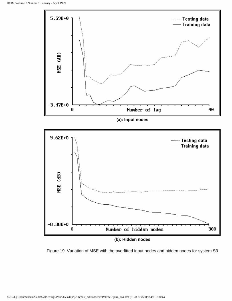
In simulated examples such as S4 where the exact input vectors are known, overfitting in the input nodes is easy to avoid. However, in real systems such as S3, the input vector is unknown, hence computing the MSE over the testing data set becomes more helpful to avoid overfitting. Furthermore, the MSE plot also gives a rough idea of the appropriate number of hidden nodes and maximum input lag. The MSE plots for S3 against the maximum number of input nodes and hidden nodes are given in Figures (19a) and (19b) respectively. The plots indicate that the network should have 80 hidden nodes and a maximum lag of 8 that is nu = 8 and ny = 8. When the network is trained using this specification

and 600 data are used for training, the correlation tests in Figure (20) are produced. All the correlation tests are satisfied, indicating that the network is adequate.



(a): Input nodes

(b): Hidden nodes

Figure 19. Variation of MSE with the overfitted input nodes and hidden nodes for system S3



Figure 20. Correlation tests of the network model with appropriate structure for system S3

Overfitted models often lose generalisation properties and give poor prediction. For instance, if the network model for system S3 is trained with an overfitted input vector and hidden nodes that are

,

and . The MPO is very bad especially over the testing data, refer to Figure (22b).

Like underfitting, overfitting also becomes more dangerous when the system is heavily corrupted by noise. In this case, the network tends to include noise as part of the process model, which often leads to a more complex model. This type of overfitted network model is often harder to detect because the network normally produces a reasonable OSA and correlation tests, however, the MPO is normally very bad. System S3 is a good example of a noisy system. The correlation tests of the overfitted network in Figure (22a) are almost as good as the correlation tests of the network with the appropriate structure in Figure (21b). However, MPO in Figure (22b) is much worse than the MPO produced using the network with the appropriate structure in Figure (21a). This is because the correlation tests are computed using OSA that is calculated over the training data set. Since the network is trained to minimise the residual over the training data set, it is not surprising that even an overfitted network will produce a good OSA over the training data set. However, OSA over the testing data set will normally deteriorate if the model is overfitted. This situation is illustrated by the OSA plot in Figure (22c).



(a): Model predicted output

(b): Correlation tests



Figure 21. Model validations of the RBF network model with the appropriate structure





(c):- One step ahead prediction

Figure 22. Model validations for the RBF network model with the overfitted structure

5. Conclusions

Various aspects of RBF network properties have been investigated using ideas from system identification and estimation theory. The network expansion reveals that the RBF network does not generate higher order lags from the specified input vector. Thus, proper input vector is vital for RBF network performance. The shapes of the basis functions have some influence on the performance of RBF network. The basis functions that have an adjustable parameter may provide better performance if the optimum value of the adjustable parameter is provided. On the other hand, the basis functions that do not have an adjustable parameter such as the thin-plate-spline and cubic functions perform reasonably well without the need for the adjustable parameter.

Three models that use the lagged u's only, lagged y's only and combinations of both lagged u's and y's were considered. It was found that the model that used both lagged u's and y's provided the most efficient model with the smallest input nodes and the best performance. The simulation results also reveal that the models that use the lagged u's or y's only, fail to represent the identified system that has multiplicative noise terms.

Network complexity is an important aspect that greatly influences RBF network performance. Both underfitting and overfitting are undesirable and often cause the network to lose the generalisation property. It was found that, the noisy data would be more sensitive to the network complexity, where a slight underfitting or overfitting may significantly affect network performance. Overfitting is difficult to detect because the overfitted network will normally give good predictions. However, prediction over the



testing data set will normally reveal the problem. The MSE plot over the testing data set will normally have a minimum, which often coincides with the true structure of the system. The results also show that the networks are more sensitive to underfitted or overfitted input vectors rather than the number of centres.

References

Billings, S.A., and Fadhil, M.B., 1985, “The practical identification of system with non-linearities”, Proc. 7th IFAC Symp. on Identification and System Parameter Estimation, York, U.K., 155-160.

Billings, S.A., and Voon, W.S.F., 1986, “Structure detection and model validity tests in the identification of non-linear systems”, Proc. IEE, Part D, 127, 272-285.

Broomhead, D.S., and Lowe, D., 1988, “Multivariable functional interpolation and adaptive networks”, Complex Systems, 2, 321-355.

Chen, S., Billings, S.A., Cowan, C.F.N., and Grant, P.M., 1990, “Non-linear systems identification using radial basis functions”, Int. J. Systems Science, 21, 2513-2539.

Chen, S., Cowan, C.F.N., and Grant, P.M., 1991, “Orthogonal least squares learning algorithm for radial basis function networks”, IEEE Trans. on Neural Networks, 2, 302-309.

Chen, S., Billings, S.A. and Grant, P.M., 1992, “Recursive hybrid algorithm for non-linear system identification using radial basis function networks”, Int. J. of Control, 55, 1051-1070.

Elanayar V.T., and Shin, Y.C., 1994, “Radial basis function neural network for approximation and estimation of non-linear stochastic dynamic systems”, IEEE Trans. on Neural Networks, 5 (4), 594-603.

Goodwin, G.C. and Payne, R.L., 1977,.Dynamic System Identification: Experiment Design and Data Analysis, Academic Press, New York.

Ljung, L., and Soderstrom, T., 1983, Theory and Practice of Recursive Identification, MIT Press, Cambridge.

Mashor, M.Y., 1995, System identification using radial basis function network, PhD thesis, University of Sheffield, United Kingdom.

Moody, J., and Darken, C.J., 1989, “Fast learning in neural networks of locally-tuned processing units”, Neural Computation, 1, 281-294.

Nahi, N.E., 1969, Estimation theory and applications, Krieger, New York.

Poggio, T., and Girosi, F., 1990, “Network for approximation and learning”, Proc. of IEEE, 78 (9), 1481-1497.

Pottmann, M., and Seborg, D.E., 1992, “Identification of non-linear processes using reciprocal multiquadratic functions”, J. of Process Control, 2 (4), 189-203.

Powell, M.J.D., 1987, “Radial basis function approximations to polynomials”, Proc. 12th



Biennial Numerical Analysis Conf., Dundee, 223-241.

Ye, X., and Loh, N.K., 1993, “Dynamic system identification using recurrent radial basis function network”, Proc. of the 1993 American Control Conf., 3, 2912-2916.

Assumption University of Thailand Huamark, Bangkok 10240 , Thailand

For comment, Please contact WebMaster


mailto:[email protected]