solving symmetric diagonally dominant linear systemsrpeng/solverslides.pdf · solving symmetric...
TRANSCRIPT

Solving Symmetric Diagonally Dominant LinearSystems
Yiannis Koutis, Gary Miller, Richard Peng

Outline

The Problem
ProblemInput: n by n matrix A with m non-zeros
vector bWhere: b = Ax for some xOutput: Approximate solution x

Types of Approaches
DirectIterativeHybrid

History of the Problem, 1st Century CE
Now known as Gaussianelimination, O(n3).

Previous Work: Direct methods
[ Strassen ‘69 ] O(n2.807).[Coppersmith-Winograd ‘90] O(n2.376).

Previous Work: Matrices with Specialized Structure
[George ‘73] Nested dissection, O(n1.5) whenthe non-zero structure is a square mesh.[Lipton-Rose-Tarjan ‘80] O(n1.5) for any planargraph using planar separators.[Alon-Yuster ‘10] Any matrix whose non-zerostructure have good separators.

Previous Work: (Purely) Iterative Methods
n: size of matrix, m: # non-zero entries.
[Hestenes-Stiefel ‘52] Conjugate gradient,O(nm).many papers Multigrid methods and othermethods studied by numerical analysts.

Laplacians
DefinitionA symmetric matrix A is a Laplacian if:
All off-diagonal entries are non-positive.All rows and columns sum to 0.

SDD Matrices
DefinitionA symmetric matrix A is Symmetric DiagonallyDominant if:
∀i Aii ≥∑j 6=i|Aij |
[Gremban-Miller ‘96] Showed solving SDD systemsis equivalent to solving Laplacians.

Laplacians
3 −1 0 0 −1 −1 0 0−1 6 −1 −1 −1 −1 −1 0
0 −1 4 −1 −1 −1 0 00 −1 −1 5 −1 −1 −1 0−1 −1 −1 −1 5 0 −1 0−1 −1 −1 −1 0 4 0 0
0 −1 0 −1 −1 0 4 −10 0 0 −1 0 0 −1 2
Corresponds to weighted graphs.Aij 6= 0 means an edge of weight −Aij betweenvertices i and j .

Laplacians
ab
cd
e
f
g
h
Corresponds to weighted graphs.Aij 6= 0 means an edge of weight −Aij betweenvertices i and j .

Previous Work: Hybrid Methods for Laplacians
n: size of matrix, m: # non-zero entries.
[Vaidya ‘89] Formalized notion of graphpreconditioners, O(m7/4).[Gremban-Miller ‘96] O(m1+ 1
2d ) ford-dimensional lattices.[Spielman-Teng ‘04] First near-linear time solver.[Koutis-Miller ‘07] O(n) work, O(n1/6) parallelruntime for planar graphs.

Near Linear Time Solver
[Spielman-Teng ‘04]
Input: n by n matrix A with m non-zerosvector b
Where: b = Ax for some xOutput: Approximate solution x s.t.
||x − x ||A < ε||x ||ARuntime: O(m log15 n log (1/ε)) expected
Technicalities: error is measured in A-norm, andruntime is cost per bit of accuracy.

Outline

Spring/Graph Embedding
Spring Mass Systems
Given a set of springs satisfying ideal physicalassumptions.Nail down some, let the rest settlePosition of rest of nodes can be calculated bysolving a Laplacian.
Spring/Graph Embedding
Tutte Embedding
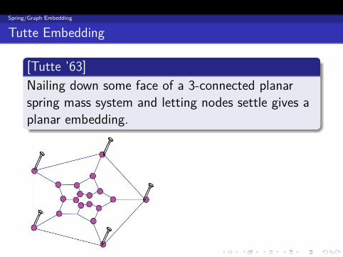
[Tutte ’63]
Nailing down some face of a 3-connected planarspring mass system and letting nodes settle gives aplanar embedding.

Spring/Graph Embedding
Learning from Labeled Data on a Directed Graph
Learning problem from labeled and unlabelleddata on a graph[Zhu-Ghahramani-Lafferty ‘03],[Zhou-Huang-Scholkopf ‘05] showed that itreduces to a SDD solve.

Related Systems
Elliptic Finite Elements PDEs
Arises in scientific computing.Partial differential equations such as heatequations, collision modelling.Discretize space into a mesh, resulting in alinear system.

Related Systems
Reduction to solving SDD systems
[Boman-Hendrickson-Vavasis ‘04]
If the mesh doesn’t have small angles, the resultinglinear system can solved with a constant number ofSDD solves.

Convex Optimization
Interior Point Methods
Minimize objective function f subject to someconstraints.Given feasible solution x , descend in somedirection.Direction chosen by solving a linear systeminvolving the Hessian matrix.

Convex Optimization
Interior Point for LP in 2D

Convex Optimization
Interior Point Method
[Karmarker], [Renagar], [Ye], [Nesterov, Nemirovsky], [Boyd,Vanderburghe] . . .
Input: Convex program with m constraintsOutput: Primal and Dual pair additive ε apartRuntime: O(
√m log (1/ε) descent steps

Convex Optimization
Interior Point and SDD Solves
[Daitsch-Spielman ‘08]
For problems such as maxflow, mincost flow, lossygeneralized flow, the linear systems involving theHessian can be computed using polylog number ofSDD solves.

Generating Random Spanning Trees
Generating Random Spanning Trees
Pick a spanning tree with equal probabilityamong all spanning trees of G .Can be Reduced to random walk sampling.Sampling only slow in certain parts of the graph.

Generating Random Spanning Trees
Speeding up random walk sampling
[Kelner-Mądry ’09]
Input: Undirected, unweighted graph GOutput: Random Spanning tree T of GRuntime: O(mn1/2).

Network Flow
Network Flow
[Christiano-Kelner-Mądry-Spielman-Teng ‘10]
Input: Undirected graph GCapacities on edges uSource vertex s, Sink vertex tError tolerance ε
Output: (1− ε) approximate maximum flow(1 + ε) approximate minimum cut
Runtime: O(m4/3)poly(1/ε)

Outline

Graph Partitioning
Sparse Cuts
Want to find a loosely connected piece.Conductance of S ⊆ V :Φ(S) = δ(S, S)/min(|S|, |S|)Want to find S that minimizes Φ(S).

Graph Partitioning
Cheeger’s Inequality
[Alon-Milman ‘85] If the optimal value is Φ,considering prefixes of the second eigenvector ofthe Laplacian gives a cut with conductance
√Φ.
[Spielman-Teng ‘96] Spectral PartitioningWorks: Planar graphs and finite element meshes.Eigenvectors can be computed using O(log n)Laplacian solves.

Graph Partitioning
Eigenvector Partition

Image Segmentation
Image Segmentation
Very related to graph partitioning.[Shi-Malik ‘01] popularized using the eigenvectorapproach
Image Segmentation
Spectral Rounding
[Koutis-Miller-Tolliver ‘06] Spectral Rounding:Find eigenvector corresponding to eigenvalue λ2.Reweigh graph edges getting a new graph.Repeat until graph is disconnected.

Image Segmentation
Medical Examples of SR
Tumors

Image Segmentation
Medical Examples of SR
Tumors

Image Denoising
Image Denoising
Given image + noise, recover image.[Rudin-Osher-Fatemi, 92] Total Variationobjective: given s, find x to minimize||s − x ||2 + λ|∇x |p.∇x calculated using a graph over the image.
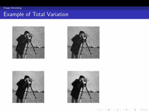
Image Denoising
Example of Total Variation

Image Denoising
Solving Total Variation
Minimize ||s − x ||2 + λ|∇x |p:p = 2: quadratic minimization, equivalent tosolving a SDD linear system.p = 1: L1 minimization, interior point algorithmcan be applied, Hessian is SDD.lag-diffusion: pretend that p = 2, then re-weightedges and iterate.

Outline

Recap: Near Linear Time Solver
[Spielman-Teng ‘04]
Input: n by n matrix A with m non-zerosvector b
Where: b = Ax for some xOutput: Approximate solution x s.t.
||x − x ||A < ε||x ||ARuntime: O(m log15 n log (1/ε)) expected

Our Result
[Koutis-Miller-P ‘10]
Input: n by n matrix A with m non-zerosvector b
Where: b = Ax for some xOutput: Approximate solution x s.t.
||x − x ||A < ε||x ||ARuntime: O(m log2 n log(1/ε)) expected
O hides a few log log n and lower terms.

More On Iterative Methods
Want to solve: Ax = bRichardson iteration:
1 u0 = 02 u(i+1) = u(i) − (b − Au(i))
Fixed point: u(i+1) = u(i) implies:b − Au(i) = 0, u(i) = x .

More On Iterative Methods
Want to solve: B−1Ax = B−1bPreconditioned Richardson iteration:
1 u0 = 02 u(i+1) = u(i) − B−1(b − Au(i))
Fixed point: u(i+1) = u(i) implies:b − Au(i) = B0, u(i) = x .

More On Iterative Methods
Want to solve: B−1Ax = B−1bPreconditioned Richardson iteration:
1 u0 = 02 u(i+1) = u(i)−B−1(b−Au(i)) Recursive Solve
Fixed point: u(i+1) = u(i) implies:b − Au(i) = B0, u(i) = x .

Rate of Convergence
Involves error term ε and the condition numberof B−1A, κ(A,B).Formally: κ(A,B) = maxx
xT AxxT Bx ·maxy
yT ByyT Ay .
Richardson’s Iteration converges inO(κ(A,B) log(1/ε).Chebyshev iteration converges inO(
√κ(A,B) log(1/ε).

What to Precondition With?
Desired properties of B:1 B−1A has low condition number.2 B is more sparse than A.

Some Bs
B = I : same as unpreconditioned.B = diag(A): Jacobi.B = upper(A): Gauss-Seidel.

Vaidya’s Paradigm Shift
[Vaidya ‘89]
Since A is a graph, B should be as well.Apply graph theoretic techniques!

What a Sparsifier Needs
Reduction in Vertex Count (dimension ofmatrix).Reduction in Edge Count (number of non-zeros).
Consider reducing edge count first.

What a Sparsifier Needs
Reduction in Vertex Count (dimension ofmatrix).Reduction in Edge Count (number of non-zeros).Consider reducing edge count first.

Edge Sparsifiers
Given a graph G , want sparse subgraph H thatpreserves some property.Spanners: distance, diameter.[Benczur-Karger ‘96] Cut sparsifier: weight of allcuts.Spectral sparsifiers: eigenstructure.

Previous Work on Spectral Sparsification
Expanders: sparsifier for complete graph.Ramanujan graphs: optimal spectral sparsifiersfor the complete graph.

Previous Work on Spectral Sparsification Algorithms
[Spielman-Teng ‘04] Spectral sparsifiers,O(n logc n) edges.[Spielman-Srivastava ‘08] Spectral sparsifiers,O(n log n) edges.[Batson-Spielman-Srivastava ‘09], derandomizedversion, O(n) edges in O(n2m) time.

What about Vertex Count?
If graph is sparse enough, can reduce vertexcount by removing vertices of degree ≤ 2 usingGaussian elimination.
Ultrasparsifier: spanning tree plus a smallnumber of edges.

What about Vertex Count?
If graph is sparse enough, can reduce vertexcount by removing vertices of degree ≤ 2 usingGaussian elimination.Ultrasparsifier: spanning tree plus a smallnumber of edges.

What We Need
UltrasparsifierInput: Graph G, n vertices, m edges.
Constant k.Output: Graph H that’s a spanning tree plus n/k edgesSuch that: Condition number of H−1G is O(k logc n).
[Spielman-Teng ‘04] with condition numberO(k logc n) implies SDD solver with runtimeO(m logc n).

What We Need
UltrasparsifierInput: Graph G, n vertices, m edges.
Constant k.Output: Graph H with n vertices, n − 1 + n/k edges.Such that: Condition number of H−1G is O(k logc n).
[Spielman-Teng ‘04] ultrasparsifier with conditionnumber O(k logc n) implies SDD solver withruntime O(m logc n).

What We Need
Ultrasparsifier Incremental SparsifierInput: Graph G, n vertices, m edges.
Constant k.Output: Graph H with n vertices, n − 1 + nm/k edges.Such that: Condition number of H−1G is O(k logc n).
[Spielman-Teng ‘04] ultrasparsifier incrementalsparsifiers with condition number O(k logc n)implies SDD solver with runtime O(m logc n).

What We Need
Incremental SparsifierInput: Graph G, n vertices, m edges.
Constant k.Output: Graph H with n vertices, n − 1 + m/k edges.Such that: Condition number of H−1G is O(k logc n).
[Spielman-Teng ‘04] incremental sparsifiers withcondition number O(k logc n) implies SDD solverwith runtime O(m logc n).

Example: Sparsifier for the Complete Graph
For Kn, 1p G(n,p) is a spectral sparsifier w.h.p. when
p ≥ log n/n.

Example: Sparsifier for the Complete Graph
For Kn, 1p G(n,p) is a spectral sparsifier w.h.p. when
p ≥ log n/n.

Generalized Graph Sampling
Flip a coin for each edge with probability ofheads being pe.If get heads, keep the edge with weightmultiplied by 1/pe.Used in cut and spectral sparsifiers.

What Sampling Gives
Expected number of edges: (∑
e pe) log n.Expected value: original graph
Concentration?

What Sampling Gives
Expected number of edges: (∑
e pe) log n.Expected value: original graphConcentration?

Effective Resistance
ab
cd
e
f
gh
Treat the graph as a circuit where each edge isa resistor with conductance wuv
For an edge e = uv , pass one unit of currentfrom u to v , resistance of the circuit is effectiveresistance, Re.

Sparsification by Effective Resistance
Theorem[Spielman-Srivastava ‘08]: If we set pe to theproduct of e’s weight and effective resistance, theresulting graph has constant condition number withthe original w.h.p.
Edge weight times effective resistance at most 1.FACT total probabilities over all edges is n − 1.Sparsifier? Ultrasparsifier? Solver?

Chicken and Egg Problem
How to calculate effective resistance?
[Spielman-Srivastava ‘08]: Use solverOur work in a nutshell: getting effectiveresistance without solver.Trick: upper bound effective resistance.

Chicken and Egg Problem
How to calculate effective resistance?[Spielman-Srivastava ‘08]: Use solver
Our work in a nutshell: getting effectiveresistance without solver.Trick: upper bound effective resistance.

Chicken and Egg Problem
How to calculate effective resistance?[Spielman-Srivastava ‘08]: Use solverOur work in a nutshell: getting effectiveresistance without solver.
Trick: upper bound effective resistance.

Chicken and Egg Problem
How to calculate effective resistance?[Spielman-Srivastava ‘08]: Use solverOur work in a nutshell: getting effectiveresistance without solver.Trick: upper bound effective resistance.

Upper Bounding Effective Resistance
ab
cd
e
f
gh
Rayleigh’s monotonicity law: as we remove edgesfrom the graph, the effective resistance between twovertices can only increase.

Upper Bounding Effective Resistance
ab
cd
e
f
gh
Rayleigh’s monotonicity law: as we remove edgesfrom the graph, the effective resistance between twovertices can only increase.

Upper Bounding Effective Resistance
ab
cd
e
f
gh
Resistors in series: effective resistance of a pathwith resistances r1 . . . rk is ∑
i ri .

Upper Bounding Effective Resistance Using Spanning Tree
Sample probability: edge weight times effectiveresistance of tree path, aka. stretch.Still gives a spectral sparsfiier
Problem: sum of probabilities no longer n − 1,sparsifier no longer have O(n log n) edges.Need to keep total stretch small.
Upper Bounding Effective Resistance Using Spanning Tree
Sample probability: edge weight times effectiveresistance of tree path, aka. stretch.Still gives a spectral sparsfiierProblem: sum of probabilities no longer n − 1,sparsifier no longer have O(n log n) edges.Need to keep total stretch small.

Choice of Tree Matters: haircomb construction
Stretch: 3

Choice of Tree Matters: haircomb construction
Stretch: 3√n edges

Choice of Tree Matters: haircomb construction
Stretch:√
n + 1

Choice of Tree Matters: haircomb construction
Stretch:√
n + 1√n edges

Choice of Tree Matters: haircomb construction
Stretch: 2√
n + 1

Choice of Tree Matters: haircomb construction
Stretch: 2√
n + 1√n edges
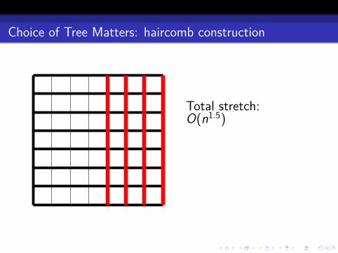
Choice of Tree Matters: haircomb construction
Total stretch:O(n1.5)

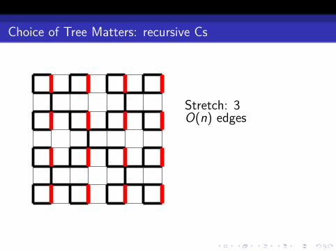
Choice of Tree Matters: recursive Cs
Stretch: 3
Choice of Tree Matters: recursive Cs
Stretch: 3O(n) edges

Choice of Tree Matters: recursive Cs
Stretch: O(√
n)

Choice of Tree Matters: recursive Cs
Stretch: O(√
n)O(√
n) edges

Choice of Tree Matters: recursive Cs
Total stretch:O(n log n).

Low Stretch Spanning Trees
Key property: total stretch S summed over alledges is small.Backbone for all known ultrasparsifiersconstructions:
[Boman-Hendrickson ‘01][Spielman-Teng ‘04 ][Kolla-Makarychev-Saberi-Teng ‘10]

Known Results on Low Stretch Spanning Trees
Theorem[Alon-Karp-Peleg-West ‘91]:A low stretch spanning tree withS = m1+ε can be constructed inO(m log n + n log2 n) time.

Known Results on Low Stretch Spanning Trees
Theorem[Elkin-Emek-Spielman-Teng ‘05]:A low stretch spanning tree withS = O(m log 2n) can be constructed inO(m log n + n log2 n) time.

Known Results on Low Stretch Spanning Trees
Theorem[Elkin-Emek-Spielman-Teng ‘05][Abraham-Bartal-Neiman ‘08]:A low stretch spanning tree withS = O(m log n) can be constructed inO(m log n + n log2 n) time.

Directly Using Low Stretch Spanning Tree
Problem: sum of probabilities S = O(m log n),too high
Trick: Sparsify a different graph
Directly Using Low Stretch Spanning Tree
Problem: sum of probabilities S = O(m log n),too highNeeds another work around
Trick: Sparsify a different graph

Directly Using Low Stretch Spanning Tree
Problem: sum of probabilities S = O(m log n),too highObservation: incremental sparsifier can be offby factor of O(k).
Trick: Sparsify a different graph

Directly Using Low Stretch Spanning Tree
Problem: sum of probabilities S = O(m log n),too highObservation: incremental sparsifier can be offby factor of O(k).Trick: Sparsify a different graph

Scale the Tree
Scale up the tree by a factor of cPay the same value in condition number.
Stretch of tree edge: 1.Stretch of non-tree Edge: reduced by factor of cto S
c .

Scale the Tree
Scale up the tree by a factor of cPay the same value in condition number.Stretch of tree edge: 1.
Stretch of non-tree Edge: reduced by factor of cto S
c .

Scale the Tree
Scale up the tree by a factor of cPay the same value in condition number.Stretch of tree edge: 1.Stretch of non-tree Edge: reduced by factor of cto S
c .

Sample After Scaling
Number of edges sampled:Tree edges: n − 1.Non-tree edges: S
c log n.Total: n − 1 + S
c log n.

Putting Things Together
Condition number: O(c) since sampling incurs aconstant factor.n − 1 + S
c = n − 1 + O(mc log2 n) edges remain.
Setting c = O(k log2 n) gives incrementalsparsifier.

Algorithm for Incremental Sparsifier Construction
IncrementalSparsify1 Find low stretch spanning tree.2 Scale up low stretch spanning tree.3 Sample by tree effective resistance.
Solver then eliminates degree 1 or 2 Nodes andrecurses.

Example of Algorithm in Action
Original graph
a
b
c
d
e
f
g
h

Example of Algorithm in Action
Find low stretch spanning tree
a
b
c
d
e
f
g
h

Example of Algorithm in Action
Scale up low stretch spanning tree
a
b
c
d
e
f
g
h

Example of Algorithm in Action
Sample by tree effective resistance
a
b
c
d
e
f
g
h

Example of Algorithm in Action
Eliminate degree 1 or 2 Nodes: h
a
b
c
d
e
f
g
h

Example of Algorithm in Action
Eliminate degree 1 or 2 Nodes: h,g
a
b
c
d
e
f
g
h

Example of Algorithm in Action
Eliminate degree 1 or 2 Nodes: h,g,e
a
b
c
d
e
f
g
h

Example of Algorithm in Action
Eliminate degree 1 or 2 Nodes: h,g,e,a
a
b
c
d
e
f
g
h

Outline

CMG Solver
Based on methods for planar graphs in[Koutis-Miller ‘07], as well as multigridtechniques.Able to solve sparse systems with 107 non-zeroentries in about a second.Package available.

Future Work
Incorporate incremental sparsifier into currentsolver code?Remove one or both of the log n factors?Error in 2-norm instead of A-norm?Extend combinatorial preconditionning to moregeneral classes of linear systems?

Thank You
Thank You