solving refinery-planning problems
TRANSCRIPT

Solving Refinery-Planning Problems
By
Arjan Buijssen [S309471]
[B.Sc. Tilburg University 2008]
A thesis submitted in partial fulfillment of the requirements for the degree of Master of Science in Operations Research and Management Science
Faculty of Economics and Business Administration Tilburg University
Supervisor university: Dr. G. Gurkan
Supervisor ORTEC: Drs. W.J. Lukje
Date: January 2008

Preface At the end of my study Econometrics and Operations Research at Tilburg University, I had to write a Master’s thesis on the area of my Master’s specialization Operations Research and Management Science. Since I did not have an internship in the first three years of my study, I really preferred to write a practical thesis based on an internship at a well-established company in the area of the Operations Research. ORTEC gave me the possibility for doing this at the Shell department. I would like to use this opportunity to thank Drs. Sandra Lukje, the supervisor from ORTEC, for all her support and involvement during the internship. There were a lot of other people from ORTEC who have also helped me with advices, information, and comments. Thank you all for helping me writing this thesis! During my internship my supervisor from the university was Dr. Gul Gurkan. I would really like to thank her for helping me writing this thesis by correcting and reading my thesis, and for pushing me in the right directions. Also special thanks go out to Prof. Dr. Ir. Dick den Hertog for introducing me to ORTEC and for being my second assessor. I would also like to thank my parents Riny and Henk for supporting me my whole life and giving me the opportunity to study and to develop myself in the way I want to. Last but certainly not least I want to thank my sister Janneke as well, for supporting me during the whole process. Arjan Buijssen Gouda, January 2008

Management Summary
In the refinery industry nonlinear programming (NLP) and linear programming (LP) problems have to be solved in all different segments of the supply chain. One sort of problem, which has to be solved for achieving a maximum profit, is the planning problem at the refinery. For optimizing these problems the optimal combination of crude oils has to be purchased, blended, and processed for selling the desired end products with a maximum profit. There are a lot of crude oils available on the market, which all have different properties (e.g. octane number, sulphur percentage, or viscosity) and prices. The end products (such as diesel and gasoline), which will be sold to the customers, have to satisfy certain specifications and demands. Due to specific parts of the optimization process, these planning problems are nonlinear. To solve these problems a software package called PIMS, specifically developed for refinery problems (by AspenTech), is used by Shell. ORTEC has been supporting Shell for more than 20 years by developing a user-interface for PIMS (called PlanStar), building the NLP models, and giving advices on these areas. Since Shell has started optimizing their refinery-planning problems with PIMS, the software has run in a mode called Distributive Recursion. In this mode the nonlinear programming problems are approximated by linear programming problems. Since a couple of years a new solving mode has been available in PIMS, which is called Extended Nonlinear Programming. This mode has a different manner of solving the nonlinear programming problems (by using a nonlinear solver). Besides this it generates additional features to analyse the obtained solutions afterwards. These additional features are useful when one wants to test the flexibility of the crude oils, to define a secondary goal (besides the primal goal of maximizing the profit), or to analyse small changes in the objective value by marginally adjusting the prices. One of the additional features can also be used in combination with a software package called Marginal Analysis Tool (developed by ORTEC and owned by Shell). One of the functionalities of this tool, which can be improved by using one of the additional features of XNLP, is to address uncertainty in the crude oil availability. It can also be utilized as a strategic tool for trading. However, according to this thesis it does not improve the functionality of the main goal of the Marginal Analysis Tool, which is to evaluate whether there are opportunities to increase the refinery margin by purchasing other crude oils than usual. Small adaptations in the feature in PIMS could also make it more useful for this purpose. A small case study also shows us that for these models XNLP does not obtain better results than DR. In most of the cases the objective values are approximately equal and the

computation times to achieve the solutions are, especially for large refinery models, larger in the XNLP mode. Hence in this thesis the mathematics and the functionality of the new nonlinear solution method XNLP available in PIMS have been investigated.
Table of Contents
Preface
Management Summary
Table of Contents
1 Introduction ............................................................................................................. 3
1.1 The petroleum industry ..................................................................................................... 3 1.2 ORTEC and Shell.............................................................................................................. 4 1.3 Problem formulation ......................................................................................................... 4
1.3.1 Optimization problems in refineries ..................................................................... 4 1.3.2 Methods of solving nonlinear problems................................................................ 5 1.3.3 Main Goal ............................................................................................................. 7 1.3.4 The approach ........................................................................................................ 7
2 Distributive Recursion .............................................................................. 9
2.1 Introduction ....................................................................................................................... 9 2.2 Pooling problem................................................................................................................ 9
2.2.1 Introduction (Example 1) ...................................................................................... 9 2.2.2 Distributive Recursion applied on pooling problem (Example 2) ...................... 13
2.3 Delta Based Modeling..................................................................................................... 18 2.3.1 Introduction ........................................................................................................ 18 2.3.2 Distributive Recursion applied on Delta Based Modeling (Example 3)............. 19
3 Extended Nonlinear Programming....................................... 29
3.1 Introduction ..................................................................................................................... 29 3.2 The CONOPT solver....................................................................................................... 30
3.2.1 GRG method ....................................................................................................... 30 3.2.2 GRG method applied on an NLP problem (Example 4) ..................................... 34
3.3 The XSLP solver ............................................................................................................. 37
4 Other packages for solving nonlinear programs.. 39
4.1 Introduction ..................................................................................................................... 39 4.2 The SNOPT solver .......................................................................................................... 39 4.3 The MINOS solver .......................................................................................................... 41 4.4 Comparison of CONOPT, XSLP, SNOPT, and MINOS................................................ 42
5 Additional output in the XNLP mode ............................... 45
5.1 Introduction ..................................................................................................................... 45 5.2 Ranging Analysis ............................................................................................................ 45
5.2.1 Introduction ........................................................................................................ 45 5.2.2 Ranging Analysis applied on a small demo model (Example 5)......................... 47
5.3 Parametric Analysis ........................................................................................................ 49 5.3.1 Introduction ........................................................................................................ 49
2
2
5.3.2 Parametric Analysis applied on a small demo model (Example 6) .................... 49 5.4 Goal Programming .......................................................................................................... 51
5.4.1 Introduction ........................................................................................................ 51 5.4.2 Goal Programming applied on a small demo model (Example 7)...................... 51
6 Case comparison ............................................................................................. 53
6.1 Introduction ..................................................................................................................... 53 6.2 Case study ....................................................................................................................... 53 6.3 Conclusions ..................................................................................................................... 54
7 Ranging Analysis in MAT .................................................................. 57
7.1 Introduction ..................................................................................................................... 57 7.2 Current method: Cargo Analysis..................................................................................... 58 7.3 Differences between both methods ................................................................................. 60 7.4 Using Ranging Analysis to improve MAT ..................................................................... 61
7.4.1 Algorithm ............................................................................................................ 61 7.4.2 Example of Ranging Analysis in MAT (Example 7)............................................ 63
7.5 Comparison of the current and new method ................................................................... 65 7.5.1 Comparison of both methods (Example 8).......................................................... 65 7.5.2 Conclusions and motivation................................................................................ 67 7.5.3 Recommendations ............................................................................................... 67
8 Conclusions and recommendations...................................... 70
8.1 Conclusions ..................................................................................................................... 70 8.2 Recommendations & further research............................................................................. 71
8.2.1 Recommendations ............................................................................................... 71 8.2.2 Further Research ................................................................................................ 72
References ....................................................................................................................... 73
Appendix A – Continuation of Example 2........................... 75
Appendix B – Continuation of Example 4 .......................... 78
Appendix C – Summary statistics of Example 5 ......... 82
Appendix D – Refineries for case study.................................. 83
Appendix E – Outcomes of Example 7 ................................... 85
Appendix F – Current implementation.................................... 88
Appendix G – Outcomes of Example 8................................... 99

3
3
1 Introduction
1.1 The petroleum industry
Oil can be defined as any substance that could be liquid that is in a viscous liquid state at ambient temperatures or slightly warmer, and is immiscible with water and miscible with other oils. It is one of the main energy resources in the world and therefore a good planned process is of great significance. Before the oil reaches its final destination, for instance the filling station, it has had a long process. Such a process is shown in Figure 1.1.
Figure 1.1 Flow diagram of the oil process
At the beginning of the process the crude oil is explored and produced at the oil fields. This will be shipped to a refinery where it will be processed, stored, and blended into different end products, such as Diesel and Premium 98. These products are then shipped (or transported through a pipeline) to a depot, from where it will be distributed to the retail, e.g. filling stations. In this thesis, the emphasis will be placed on the refinery part of the process. A refinery can be defined as a complex of factories, pipelines, and tanks that transform the crude oil into many useful products like LPG, Diesel, and Gasoline. At such a refinery, many essential decisions have to be taken, in such a way that the correct end products will be produced with a maximum total profit. In Section 1.2 the role of ORTEC and Shell in this process will be discussed and in Section 1.3 the problem of this thesis will be described and formulated.
crude processing storage blending
shipping
depot distribution retail customer
4
4
1.2 ORTEC and Shell
ORTEC is one of the largest providers of advanced planning and optimization solutions. Founded in 1981, ORTEC currently has more than 500 employees and offices in North America and Europe. Their blue-chip customer base of more than 800 customers includes leading enterprises in manufacturing, transportation, industry and banking. ORTEC is a privately held company that develops, markets, and implements advanced planning and scheduling software, according to http(1). Most of the employees work at the office in Gouda. One of the business units at this office is ‘ORTEC Logistics Consulting’, in which for small regional companies as well as multi-national corporations the logistic operations and processes are improved. With the aid of the experts at ORTEC, unique opportunities can be identified to improve their logistics network, according to http(6). The largest department in this business unit is fully arranged for the support of Shell, a worldwide group of oil, gas, and petrochemical companies. This thesis is written on the basis of an internship at this department. At this department nearly the complete supply chain is optimized with the aid of ORTEC. The part of the supply chain discussed in this thesis is the planning process from the crude oil selection until the selling process at the gate of the refinery (from crude until blending in Figure 1.1), without taking the transportation of the products to the customers into account. One of the projects in the Shell department is the development of software packages for Shell to help optimizing their crude oil selection, the process of refining, and blending possibilities at the refineries. A more detailed description of the problems that occur at a refinery and the corresponding optimization methods is stated in Section 1.3.
1.3 Problem formulation
1.3.1 Optimization problems in refineries
An optimization problem is a computational problem in which the goal is to find the best of all possible solutions. More formally, the objective is to find a solution in the feasible region, which has the optimal value of the objective function. Such problems occur everywhere and therefore also in the petroleum world. The complete supply chain of the petroleum industry will not be discussed in this thesis, but only the part at the refineries. As explained above, a petroleum refinery is a complex of factories, pipelines, and tanks that transforms raw materials (crude oil) into many useful end products. There are many different crude oils, which all have various properties and molecule structures. When a certain crude oil enters the refinery, it will be processed in several processing units. These units transform the crude oil into intermediates, called components. After these processes the intermediates will be blended in the right proportion to obtain the desired products, specified by the customer. To get an idea of all these processes in a refinery, an example of a flow diagram of a rather complex refinery is shown in Figure 1.2.

5
5
Figure 1.2 Flow diagram of a petroleum refinery
As shown in this figure, the crude oils are first processed into components like LPG, Naptha, and Kerosine, using a Crude Distilling Unit. After that, several units, such as a Hydro Treater, Platformer, and High Vacuum Unit, are used to transform these components into products with the user-preferred properties, like sulphur percentage, octane number, and density. The crude oil costs are about 90% of the refinery input cost and therefore the selection of the optimal crude oil mix is extremely important to achieve higher profits. Due to the diversity of the crude oils and the corresponding fluctuating price scenarios, it is very difficult to evaluate all possible scenarios to obtain the optimum crude oil mix for the refinery. Besides this, also the streams inside the refineries are extremely diverse. Modeling these processes therefore results in nonlinear programming problems. In Subsection 1.3.2 the methods for dealing with the nonlinearity of these problems will be discussed in more detail.
Note that also the transportation of the crude oils to the refinery is subject to a lot of uncertainty, such as cargo sizes, sea routes etcetera. However, this will be considered as given in the rest of this thesis.
1.3.2 Methods of solving nonlinear problems
There are many unknown variables in a petroleum refinery that are influencing the total profit of the refinery, such as crude oil purchases, product sales, and the division of the amounts to the different units. To obtain the optimal allocation of these variables, a mathematical representation of the process can be developed. The best approximation of such a process is a nonlinear programming (NLP) problem, since in practice several complex nonlinear parts are involved in the problem. However, nonlinear problems could be very difficult mathematical problems and are most of the time very hard or even impossible to solve. At this moment many software packages are on the market to deal with these nonlinear problems. One of those packages is called “PIMS”, which has been developed by

6
6
AspenTech. Shell utilizes this package to solve and evaluate the planning problems at their refineries worldwide. ORTEC advises Shell on the area of quantitative optimization problems. In Figure 1.3 three programs are shown that are developed by ORTEC and owned by Shell Global Solutions, to simplify the use of PIMS and to analyse solutions obtained by PIMS.
Figure 1.3 Flow diagram of FE, MAT, PlanStar and PIMS
Since PIMS is a complicated software package, PlanStar has been built as a user-interface to simplify PIMS for the users. PlanStar, developed by ORTEC, is a refinery-planning tool, containing a graphical user interface and a database that stores all the required data. It exports the data to PIMS and shows the obtained solution afterwards in a clarifying way. Hence note that PlanStar does not solve the nonlinear problem itself.
Besides PlanStar, ORTEC has also developed the two Microsoft Excel templates ‘Front-End’ (FE) and ‘Marginal Analysis Tool’ (MAT). The Front-End is used for defining and updating primarily commercial data for the monthly plan. Thus it prepares a base case in Excel, which can be imported in PlanStar, followed by the optimization step in PIMS and the import of the solution in PlanStar afterwards. With an optimal monthly plan available in PlanStar, MAT is used for analysing the optimal solution by marginal changes of decision variables or parameters. The principle of MAT is to change only one item per case, leaving the rest of the model unchanged. MAT consists of two parts: Cargo Analysis and Marginal Steering. In Cargo Analysis the user can analyse cases with a different crude oil (or other feedstock) composition. On the other hand, in Marginal Steering cases can be defined with marginal changes in for instance unit capacities or product demands. The cases setup in MAT can be returned to PlanStar and optimized by using PIMS. Shell is using PIMS to solve their nonlinear optimization problems at the refinery. The solution method that is used in PIMS is called Distributive Recursion (DR). Since 2003 there has been a new nonlinear method available in PIMS, called Extended Nonlinear Programming (XNLP). According to the developers, this method performs faster and gives more global optima than Distributive Recursion. Shell is questioning whether or not transforming their refinery models to be solved in the XNLP mode, since the functionality and the mathematics behind it can be seen as a black box. Therefore they want to
7
7
investigate the (dis)advantages of this method, to decide switching from the DR to the XNLP mode.
1.3.3 Main Goal
The main goal of this thesis can be formulated as follows: To investigate the mathematics and the functionality of the new nonlinear solution method XNLP available in PIMS. This main goal can be achieved by answering the following research questions:
• How do the two solution methods Distributive Recursion and Extended Nonlinear Programming work on mathematical level?
• How appropriate are the nonlinear solvers that are available in XNLP for solving refinery-planning problems, compared to other main nonlinear solvers?
• To what extent does XNLP provide more accurate and higher quality solutions in the refinery planning area?
• What are the additional features when using XNLP and how can they be used to improve the functionality of the Marginal Analysis Tool?
1.3.4 The approach
To fulfill the main goal of this thesis, the old method Distributive Recursion first has to be discussed extensively to get a good overview of the current situation. The method will also be applied on some small examples, which contain typical nonlinear parts of a refinery-planning model. This mathematical discussion of the Distributive Recursion is in Chapter 2. After the overview of the current situation has been given, the mathematical background of the new method XNLP will be discussed. The user can choose between two nonlinear solvers (inside this method) to solve the problems, namely CONOPT and XSLP. They both have to be discussed to get a good overview of the new situation and to provide an answer to the first research question, which is done in Chapter 3 of this thesis. After this mathematical discussion, the question arises why the solvers CONOPT and XSLP are available in the XNLP mode, although there are many other nonlinear solvers available on the market. It therefore has to be investigated to what extent these two nonlinear solvers are appropriate for refinery-planning problems, compared to two other nonlinear solvers SNOPT and MINOS. To provide a good answer to the second research question, this will be investigated in Chapter 4. Since Extended Nonlinear Programming is based on a different mathematical method than Distributive Recursion, it may also generate other, additional features to analyse the obtained solution. In Chapter 5 of this thesis these features will be investigated, such that the first part of the fourth research question could be answered. After these chapters, the basic theoretical background of both solution methods DR and XNLP is clarified. A good continuation of this thesis is now to compare both methods in a practical way by using some nonlinear programming (NLP) problems of refineries of Shell (see Chapter 6). In this chapter the third research question “To what extent does XNLP

8
8
provide more accurate and higher quality solutions in the refinery planning area?” will be investigated. The utility of the additional features, which may be generated by using XNLP, also has to be investigated. This is done in Chapter 7, such that it will be attempt to provide a reliable answer to the second part of the fourth question “How can the additional features be used to improve the functionality of the Marginal Analysis Tool?”.
9
9
2 Distributive Recursion
2.1 Introduction
Since the beginning of the petroleum industry, companies have been searching for the best possible method for solving the (nonlinear) problems at the refineries. The main issue of nonlinear programming problems is the fact that a final solution, which has been obtained by a certain solver, in the absence of certain mathematical properties (such as convexity), may be a local optimum. Hence, a solver can distinguish itself from others by obtaining global optima more frequently as final solution. Since 1980, Shell (one of the largest worldwide group of oil, gas, and petrochemical companies) has used Distributive Recursion in combination with the software package of AspenTech (PIMS). Distributive Recursion is a specific version of Successive Linear Programming (SLP), where the nonlinear problem is represented in PIMS as a linear problem, by presuming some of the variables as known. After solving the linear problem, the presumed value and calculated physical value are compared, which results in a certain “error”. If this error is not sufficiently small, the guessed variables are updated and a new LP is solved. This method of solving nonlinear problems will be explained in more detail in Section 2.2 and it will be applied on the (nonlinear) pooling problem in refineries. In Section 2.3 it will be applied on a more complicated and advanced problem that occurs in refineries (Delta Based Modeling).
2.2 Pooling problem
2.2.1 Introduction (Example 1)
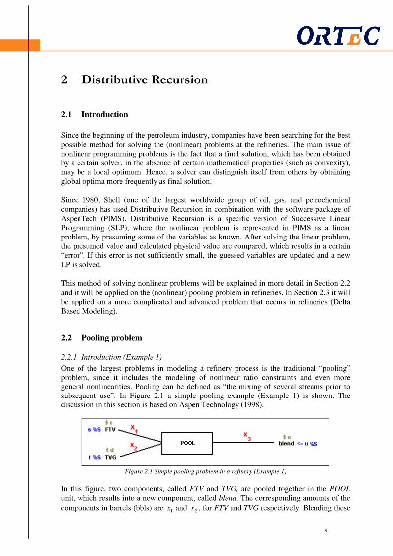
One of the largest problems in modeling a refinery process is the traditional “pooling” problem, since it includes the modeling of nonlinear ratio constraints and even more general nonlinearities. Pooling can be defined as “the mixing of several streams prior to subsequent use”. In Figure 2.1 a simple pooling example (Example 1) is shown. The discussion in this section is based on Aspen Technology (1998).
Figure 2.1 Simple pooling problem in a refinery (Example 1)
In this figure, two components, called FTV and TVG, are pooled together in the POOL unit, which results into a new component, called blend. The corresponding amounts of the
components in barrels (bbls) are 1x and 2x , for FTV and TVG respectively. Blending these

10
10
.
2000
2000
321
2
1
xxx
x
x
=+
≤≤
≤≤
two components results in an amount 3x of blend, which is the sum of 1x and 2x .
Furthermore, every component in the process has certain properties, which are typical for that component, like density, sulphur percentage, and viscosity. For the sake of this example, we will focus only on the sulphur percentage (%S) of the components, which is denoted by s and t (in %S), for FTV and TVG respectively. The sulphur percentage of the blend has been restricted to a certain percentage denoted by u (in %S), which means that not every ratio between the amounts of the two incoming components has been allowed. In Figure 2.1 the purchasing prices of the components FTV and TVG are denoted by c and d (in $/bbl) respectively. The selling price of blend is denoted by e (in $/bbl). The goal of
this problem is to purchase the components FTV and TVG (determining values for 1x and
2x ) in such a way that the total profit has been maximized and the sulphur constraint does
not violate. To illustrate this example, the values for the parameters are shown in Table 2.1.
Parameter Value
c $2
d $3
e $4
s 1.5 %S
t 0.5 %S
u 1 %S
Table 2.1 Numerical parameter values (Example 1)
Note that the problem does not take into account properties such as the density of the different components, since such properties would make the example more complicated and thus less comprehensible. The objective of this problem is to maximize the total profit, thus it has the following objective function:
213 324max xxx −− .
Let us assume that the refinery is not allowed to buy more than 200 barrels of each component. Since every component has different properties (in this case: sulphur percentages), the ratio between these quantities is essential for the outcomes of the problem. However, the ratio in this mixture is not known in advance. The optimal ratio, which maximizes the total profit, is restricted by quantity and quality constraints. As the
name implies, quantity constraints are restrictions on the quantities of the variables 1x , 2x ,
and 3x . These constraints are in this example defined as:
(2.1)
The quality constraints concern some specifications of the components, for instance the sulphur content or the Research Octane Number (RON). In this case, the blend has the

11
11
restriction that it is not allowed to contain more than 1 %S sulphur. Hence the quality constraint can be defined as:
12123
21
21 ≤+
+
xx
xx.
Now the total problem can be rewritten into the following LP problem:
.2000
2000
2max
2
1
21
21
≤≤
≤≤
≤
+
x
x
xx
xx
To see this, note that the third constraint of (2.1) can be used to simplify the objective function. As one can see, the described problem is linear and therefore solvable with a linear solver. A simple calculation gives us an objective function value of 800 with
corresponding values 2001 =x and 2002 =x (maximum allowable values).
However, when the problem of Figure 2.1 is enlarged, a nonlinear constraint will arise. The enlarged problem (Example 2) is shown in Figure 2.2.
Figure 2.2 Enlarged pooling problem in a refinery (Example 2)
The notation that has been used in Figure 2.2 is stated in Table 2.2.
Notation Description
1c Cost SRS ($/bbl)
2c Cost FTV ($/bbl)
3c Cost TVG ($/bbl)
ap Price blend a ($/bbl)
bp Price blend b ($/bbl)
1q Sulphur content SRS (%S)
2q Sulphur content FTV (%S)
3q Sulphur content TVG (%S)
aq Sulphur content blend a (%S)

12
12
.)4(
)4(
0)4(
0)4(
0)4(
)3(
)2(
)1(
)1(
)(max
5
41
33
22
11
5432
32
3322
5
5
41
411
332211541
b
a
b
b
b
ba
lxe
lxxd
uxc
uxb
uxa
xxxx
qxx
xqxq
bx
xqb
axx
xqxqa
xcxcxcxpxxp
≥
≥+
≤≤
≤≤
≤≤
+=+
=+
+
≤
≤+
+
−−−++
bq Sulphur content blend b (%S)
a Upperbound quality blend a
b Upperbound quality blend b
1u Upperbound quantity SRS (bbls)
2u Upperbound quantity FTV (bbls)
3u Upperbound quantity TVG (bbls)
al Lowerbound quantity blend a (bbls)
bl Lowerbound quantity blend b (bbls)
1x Quantity SRS (bbls)
2x Quantity FTV (bbls)
3x Quantity TVG (bbls)
4x Quantity of POOL directed to blend a (bbls)
5x Quantity of POOL directed to blend b (bbls)
Table 2.2 Notation table of the pooling problem (Example 2)
In this case, all costs, prices, qualities (sulphur percentages) of the components, and bounds are parameters and thus given. The decision variables to be optimized in this
nonlinear problem are basically 1x , 2x , 3x , 4x , and 5x . Again, these variables have to be
chosen in such a way that the total profit will be maximized. Using Figure 2.2 and Table 2.2, the following mathematical model of the optimization problem can be developed:
(2.2)
In this model the total profit is once more the difference between the revenue and the total costs restricted to quality and quantity constraints, as shown in (2.2). The constraints (1a) and (1b) are the quality constraints of the two blends; constraint (2) is the quality
13
13
.
0
0
0
)(
)(
)(max
5
41
33
22
11
5432
323322
414
32
332211
54332211
b
a
baa
lx
lxx
ux
ux
ux
xxxx
xxbxqxq
xxaxxx
xqxqxq
xpxpxcxcxcp
≥
≥+
≤≤
≤≤
≤≤
+=+
+≤+
+≤+
++
++−−−
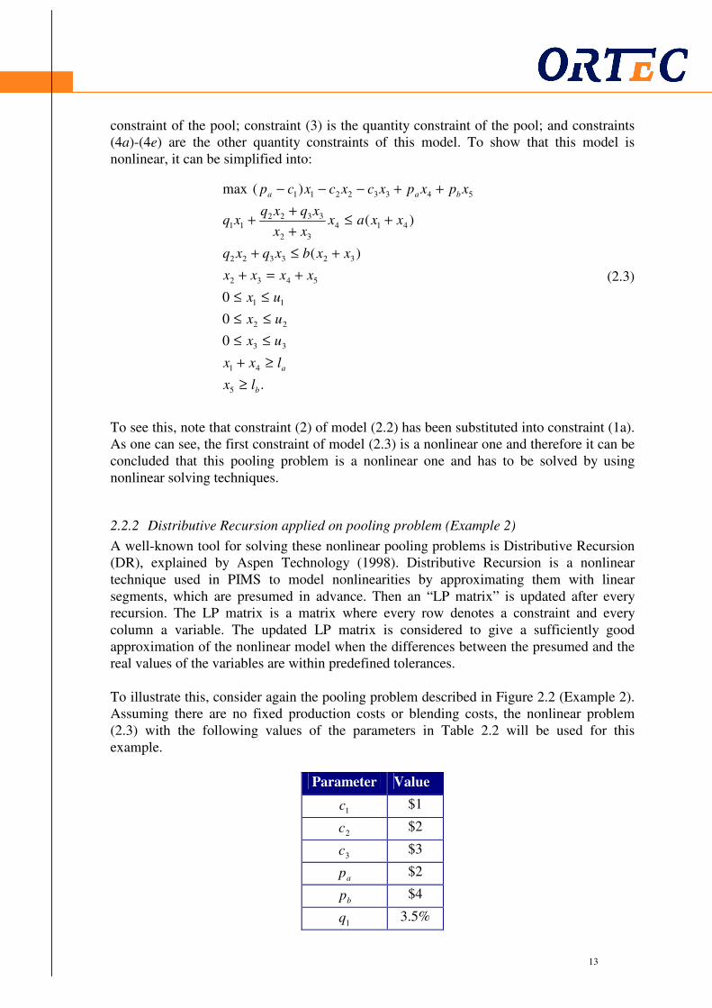
constraint of the pool; constraint (3) is the quantity constraint of the pool; and constraints (4a)-(4e) are the other quantity constraints of this model. To show that this model is nonlinear, it can be simplified into:
(2.3)
To see this, note that constraint (2) of model (2.2) has been substituted into constraint (1a). As one can see, the first constraint of model (2.3) is a nonlinear one and therefore it can be concluded that this pooling problem is a nonlinear one and has to be solved by using nonlinear solving techniques.
2.2.2 Distributive Recursion applied on pooling problem (Example 2)
A well-known tool for solving these nonlinear pooling problems is Distributive Recursion (DR), explained by Aspen Technology (1998). Distributive Recursion is a nonlinear technique used in PIMS to model nonlinearities by approximating them with linear segments, which are presumed in advance. Then an “LP matrix” is updated after every recursion. The LP matrix is a matrix where every row denotes a constraint and every column a variable. The updated LP matrix is considered to give a sufficiently good approximation of the nonlinear model when the differences between the presumed and the real values of the variables are within predefined tolerances. To illustrate this, consider again the pooling problem described in Figure 2.2 (Example 2). Assuming there are no fixed production costs or blending costs, the nonlinear problem (2.3) with the following values of the parameters in Table 2.2 will be used for this example.
Parameter Value
1c $1
2c $2
3c $3
ap $2
bp $4
1q 3.5%
14
14
2q 1.5%
3q 0.5%
a 2
b 1
1u 200
2u 200
3u 200
al 100
bl 100
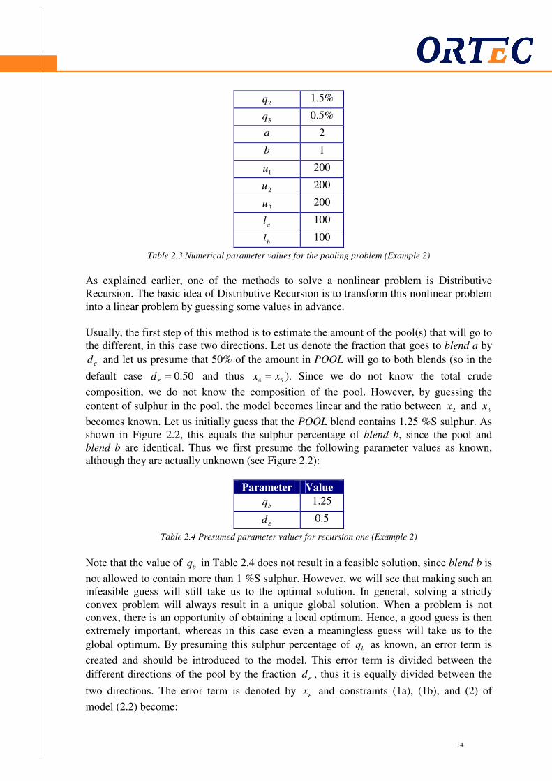
Table 2.3 Numerical parameter values for the pooling problem (Example 2)
As explained earlier, one of the methods to solve a nonlinear problem is Distributive Recursion. The basic idea of Distributive Recursion is to transform this nonlinear problem into a linear problem by guessing some values in advance. Usually, the first step of this method is to estimate the amount of the pool(s) that will go to the different, in this case two directions. Let us denote the fraction that goes to blend a by
εd and let us presume that 50% of the amount in POOL will go to both blends (so in the
default case 50.0=εd and thus 54 xx = ). Since we do not know the total crude
composition, we do not know the composition of the pool. However, by guessing the
content of sulphur in the pool, the model becomes linear and the ratio between 2x and 3x
becomes known. Let us initially guess that the POOL blend contains 1.25 %S sulphur. As shown in Figure 2.2, this equals the sulphur percentage of blend b, since the pool and blend b are identical. Thus we first presume the following parameter values as known, although they are actually unknown (see Figure 2.2):
Parameter Value
bq 1.25
εd 0.5
Table 2.4 Presumed parameter values for recursion one (Example 2)
Note that the value of bq in Table 2.4 does not result in a feasible solution, since blend b is
not allowed to contain more than 1 %S sulphur. However, we will see that making such an infeasible guess will still take us to the optimal solution. In general, solving a strictly convex problem will always result in a unique global solution. When a problem is not convex, there is an opportunity of obtaining a local optimum. Hence, a good guess is then extremely important, whereas in this case even a meaningless guess will take us to the
global optimum. By presuming this sulphur percentage of bq as known, an error term is
created and should be introduced to the model. This error term is divided between the
different directions of the pool by the fraction εd , thus it is equally divided between the
two directions. The error term is denoted by εx and constraints (1a), (1b), and (2) of
model (2.2) become:

15
15
This error term is necessary for calculating the real sulphur percentage of the pool ( bq ).
Now the linear problem to be solved by using model (2.2) and assuming the parameter values and guesses discussed above, becomes:
(2.4)
This model can be rewritten into matrix form (with constraints on the rows and variables
on the columns) and solved using a linear solver (like Xpress or CPlex), in which 1x , 2x ,
3x , 4x , 5x , and εx are the decision variables. It results in the solution shown in Table 2.5.
Variable Activity (barrels per day)
1x 61.53
2x 92.31
3x 200
4x 38.47
5x 253.86
εx -126.92
Optimal Value ($)
Objective 369.23
Table 2.5 Optimal solution of recursion one (Example 2)
First note that the value of the variable is usually denoted by ‘the activity’ of the variable. Also note that this first solution is in most of the cases not directly the optimal solution of the pooling problem. This is due to the guesses and the nonlinearity of the original problem.
.)5(
100)4(
2000)4(
2000)4(
2000)4(
100)4(
)3(
)(25.15.05.1)2(
5.025.1)1(
)(25.025.15.3)1(
4232max
5
3
2
1
41
5432
3232
55
4141
54321
ℜ∈
≥
≤≤
≤≤
≤≤
≥+
+=+
++=+
≤+
+≤++
++−−
ε
ε
ε
ε
x
xe
xd
xc
xb
xxa
xxxx
xxxxx
xxxb
xxxxxa
xxxxx
.)()2(
)1()1(
)()1(
323322
55
41411
ε
εε
εε
xxxqxqxq
bxxdxqb
xxaxdxqxqa
b
b
b
++=+
≤−+
+≤++
16
16
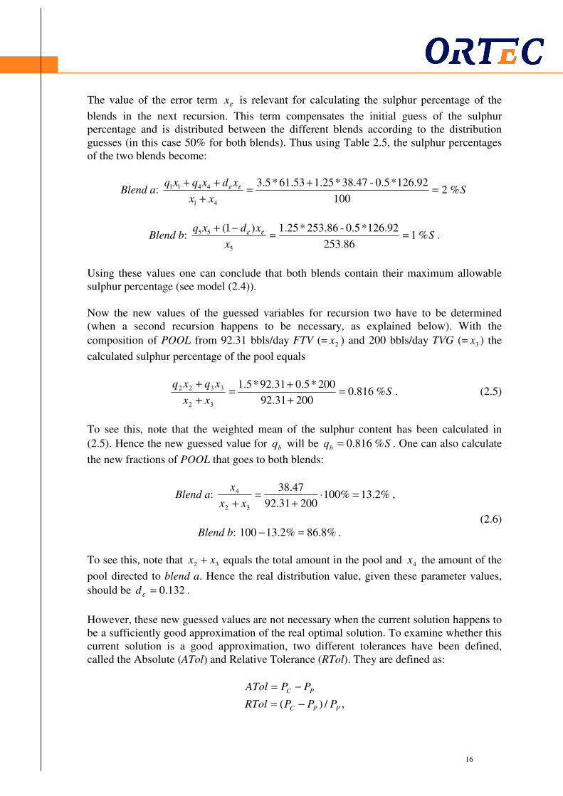
The value of the error term εx is relevant for calculating the sulphur percentage of the
blends in the next recursion. This term compensates the initial guess of the sulphur percentage and is distributed between the different blends according to the distribution guesses (in this case 50% for both blends). Thus using Table 2.5, the sulphur percentages of the two blends become:
Blend a: Sxx
xdxqxq%2
100
126.92*0.5-38.47*1.2561.53*3.5
41
4411 =+
=+
++ εε
Blend b: Sx
xdxq%1
253.86
126.92*0.5-253.86*1.25)1(
5
55 ==−+ εε .
Using these values one can conclude that both blends contain their maximum allowable sulphur percentage (see model (2.4)). Now the new values of the guessed variables for recursion two have to be determined (when a second recursion happens to be necessary, as explained below). With the
composition of POOL from 92.31 bbls/day FTV (= 2x ) and 200 bbls/day TVG (= 3x ) the
calculated sulphur percentage of the pool equals
Sxx
xqxq%816.0
20031.92
200*5.031.92*5.1
32
3322 =+
+=
+
+. (2.5)
To see this, note that the weighted mean of the sulphur content has been calculated in
(2.5). Hence the new guessed value for bq will be Sqb %816.0= . One can also calculate
the new fractions of POOL that goes to both blends:
Blend a: %2.13%10020031.92
47.38
32
4 =⋅+
=+ xx
x,
(2.6) Blend b: %8.86%2.13100 =− .
To see this, note that 32 xx + equals the total amount in the pool and 4x the amount of the
pool directed to blend a. Hence the real distribution value, given these parameter values,
should be 132.0=εd .
However, these new guessed values are not necessary when the current solution happens to be a sufficiently good approximation of the real optimal solution. To examine whether this current solution is a good approximation, two different tolerances have been defined, called the Absolute (ATol) and Relative Tolerance (RTol). They are defined as:
,/)( PPC
PC
PPPRTol
PPATol
−=
−=

17
17
where CP denotes the current property value and PP the previous property value. Usually,
the default value for each tolerance is 0.001. In our example, we only focus on the sulphur property, so only for that property these tolerances can be calculated. After recursion one we obtain the following values for ATol and RTol:
.001.03474.025.1
25.1816.0
001.04342.025.1816.0
>=−
=
>=−=
RTol
ATol
Since neither the ATol nor the RTol is less than the allowed tolerance, a new recursion has to be executed, with the updated values of the non-converged property values. According to (2.5) and (2.6), the new guess of the sulphur percentage in the pool will become 0.816 (instead of 1.25) and the new proportion of the direction of POOL will become 13.2% to blend a and 86.8% to blend b (instead of both 50%). Thus model (2.4) will be adjusted by presuming the following values as known:
Parameter Value
bq 0.816
εd 0.132
Table 2.6 Presumed parameter values for recursion two (Example 2)
With these values, the new linear programming problem can be solved similarly as describe above. This will result in new activities for all the decision variables, a new value
of εd , and new actual sulphur percentages for both blends. These values can be tested
again, using to the tolerances described above. If necessary, more recursions can be run until a sufficiently good approximation of the nonlinear programming problem has been obtained. The elaboration of these recursions is similar to the first one and therefore stated in Appendix A. After three recursions, the obtained solution proves to be a sufficiently good approximation of the NLP problem. The corresponding outcomes are stated in Table 2.7.
Variable Activity (barrels per day)
1x 40
2x 200
3x 200
4x 60
5x 340
Optimal Value (dollar)
Objective 520
Guessed values
bq 1 %S
εd 0.150
Table 2.7 Optimal solution of the pooling problem, determined with Distributive Recursion (Example 2)

18
18
In the next section this example will be enlarged with a so-called “base + delta”-unit, which makes Distributive Recursion a bit more complicated.
2.3 Delta Based Modeling
2.3.1 Introduction
Another complex part of the process at the refineries is addressed by Delta Based Modeling (DBM). DBM is a linear programming technique used for predicting yields of processing units and their corresponding properties, in situations where these yields and properties are a function of feed quality d therefore unknown in advance. Notice once more that the methods explained in this thesis are applied on static models, to plan the purchases and sells of a certain period (e.g. month) for a petroleum refinery. DBM is usually applied on models with a large amount of streams, since it reduces the complexity of the model. However, this complexity reduction causes a loss in information about the use of particular streams in the refinery. We next explain DBM in more detail, based on Aspen Technology (1998). Delta Based Modeling is applied on a so called “base + delta”-unit. The main difference between a pooling unit (as explained in Section 2.2) and a “base + delta”-unit, is the process inside the unit. In the former unit, a linear process takes place, which results in linear equations to calculate the qualities (like sulphur percentages) and quantities of the outgoing stream. Though note that the complete model is still nonlinear (as described in Section 2.2). On the other hand, in a “base + delta”-unit the qualities of the outgoing streams cannot be calculated by using linear equations, since several chemical reactions take place inside. For instance, the total sulphur of the incoming stream does not have to equal the total sulphur of the outgoing stream, in contrast with the model discussed in Section 2.2. Such a unit is usually preceded (or fed) by a pool of streams, i.e. fed by a component with an unknown composition, which has to be determined by the optimization
process (e.g. stream 5x in Example 2). Hence the properties (and yields) of the feed of the
unit are unknown for the user. As a consequence, the properties and yields of the outgoing streams of the unit will also be unknown in advance, which makes it more complicated to model. It implies that these processing units have to be modeled in such a way that they can cope with these unknown properties and yields. Therefore, Delta Based Modeling combined with Distributive Recursion is applied to predict the yields and properties of these outlet streams, by approximating the real process by a linearization of the data. This concept is illustrated in Figure 2.3.

19
19
Figure 2.3 Delta Based Modeling
In Figure 2.3 the property value (e.g. sulphur percentage) of a certain incoming stream is shown on the x-axis. On the y-axis the corresponding yield of the outgoing stream is shown when it has been processed in the “base + delta”-unit. The real data for a certain property is unknown. However, assuming there is appropriate empirical data, a regression line of this data can be drawn, which will be used to approximate the real data. This regression line is the linearized data as shown in the figure. As one can see, the linearized data is an approximation of the real data. The user must be satisfied that the slopes of the curves used in this method reflect a linear relationship between the yield and the property value and that this relationship adequately models the real world for each specific DBM application. Since the modeling and solving of a huge amount of streams could be very complex, DBM pre-estimates some unknown variables such that the model can be solved by using Distributive Recursion. Thus in addition to Example 2 (see Section 2.2), more variables will be presumed as known. In Subsection 2.3.2 this will be shown by using an extension of Example 2.
2.3.2 Distributive Recursion applied on Delta Based Modeling (Example 3)
To apply the Distributive Recursion method together with Delta Based Modeling, an extension of Example 2 will be used. This extension, Example 3, is shown in Figure 2.4.
Figure 2.4 Pooling unit together with a “base + delta” unit (Example 3)
In contrast with Example 2, one of the two directions downstream the pool cannot be sold directly to the customer, but is progressed to a “base + delta”-unit. Inside this unit a certain chemical process takes place. The details of the exact process are beyond the scope of this

20
20
thesis. An example of such a unit is a ‘Hydro-Desulphurizer unit’, where the pool stream
5x (with a high sulphur percentage) is converted into fuels with lower sulphur percentages
( 6x and 7x ). As a consequence of this new unit, blend b is not sold anymore. Instead, two
new end products DIESEL and GASOLINE have been added and can be produced and sold now. Note that these products also have quantity and quality (sulphur percentage) constraints. The notation in Figure 2.4 is comparable with those of Figure 2.2. For simplicity, the parameters with corresponding values and the decision variables are shown in Table 2.8.
Notation Description Value
1c Cost SRS ($/bbl) $1
2c Cost FTV ($/bbl) $2
3c Cost TVG ($/bbl) $3
ap Price blend a ($/bbl) $2
Dp Price DIESEL ($/bbl) $6
Gp Price GASOLINE ($/bbl) $5
1q Sulphur content SRS (%S) 3.5 %S
2q Sulphur content FTV (%S) 1.5 %S
3q Sulphur content TVG (%S) 0.5 %S
Pq Sulphur content outgoing stream of the pool (thus
of 4x and 5x ) (%S)
Decision variable
Dq Sulphur content DIESEL (%S) Decision variable
Gq Sulphur content GASOLINE (%S) Decision variable
1u Upperbound quantity SRS (bbls) 200
2u Upperbound quantity FTV (bbls) 200
3u Upperbound quantity TVG (bbls) 200
a Upperbound quality blend a (%S) 2 %S
b Upperbound quality DIESEL (%S) 0.4 %S
c Upperbound quality GASOLINE (%S) 1.5 %S
al Lowerbound quantity blend a (bbls) 100
Dl Lowerbound quantity DIESEL (bbls) 0
Gl Lowerbound quantity GASOLINE (bbls) 0
1x Quantity SRS (bbls) Decision variable
2x Quantity FTV (bbls) Decision variable
3x Quantity TVG (bbls) Decision variable
4x Quantity out of POOL directed to blend a (bbls) Decision variable
5x Quantity out of POOL directed to UNIT (bbls) Decision variable
6x Quantity out of POOL directed to DIESEL (bbls) Decision variable
7x Quantity out of POOL directed to GASOLINE (bbls) Decision variable
Table 2.8 Notation table (Example 3)

21
21
,)5(
)5(
)5(
0)5(
0)5(
0)5(
),()4(
),()4(
)3(
)3(
)2(
)1(
)1(
)1(
)(max
7
6
41
33
22
11
7
6
765
5432
32
3322
7
7
6
6
41
411
3322117641
G
D
a
PG
PD
P
G
D
P
GDa
lxf
lxe
lxxd
uxc
uxb
uxa
xqgqb
xqfqa
xxxb
xxxxa
qxx
xqxq
cx
xqc
bx
xqb
axx
xqxqa
xcxcxcxpxpxxp
≥
≥
≥+
≤≤
≤≤
≤≤
=
=
+=
+=+
=+
+
≤
≤
≤+
+
−−−+++
This model can be represented as a nonlinear programming problem, where the total profit has to be maximized without violating the quality and quantity constraints. It results in the following NLP problem:
(2.7)
where f and g are unknown, nonlinear functions. In comparison with the model of
Example 2 (model (2.4)), some constraints have been changed and some new ones have been defined. To clarify these modifications, all constraints are briefly discussed below:
• Constraints (1a) – (1c): These constraints are the quality (sulphur) constraints of the different products, i.e. for every product there is a maximum percentage of sulphur allowed. Quality constraint (1a) is the one for blend a, (1b) for DIESEL, and (1c) for GASOLINE.
• Constraint (2): This constraint is the quality constraint of the pool unit. It can be interpreted as the condition that the weighted sulphur percentage of the pool has to equal the sulphur percentage of the outgoing stream (which is a decision variable).
• Constraints (3a) – (3b): These are the quantity constraints of the units POOL and UNIT respectively. In these constraints it is stated that the total weight of the incoming stream has to equal the total weight of the outgoing stream.
• Constraints (4a) – (4b):
22
22
These two constraints are the quality constraints for the two end products DIESEL and GASOLINE. In these constraints it is stated that the sulphur percentages of DIESEL
( Dq ) and GASOLINE ( Gq ) are (nonlinear) functions of the quality of the input in the
unit ( Pq ) and the amount that is directed to the product ( 6x or 7x ). These functions are
unknown (see the real data in Figure 2.3), due to the fact that the process inside the “base + delta”-unit is not given. Notice again that in such a unit, the total sulphur of the incoming stream does not have to be equal to the total sulphur of the outgoing stream, since it could be for instance a ‘Hydro-Desulphurizer unit’. Therefore, the function is unknown and will be linearized by using Delta Based Modeling (see the linearized data in Figure 2.3). In addition, it is known that when we estimate (or guess) the quality of
the input ( Pq ), the functions f and g become linear. Thus f and g are linear in 6x and 7x
respectively.
• Constraints (5a) – (5f): These quantity constraints are the sell and purchase constraints. So, for all the crude oils that can be purchased, there is the ability of choosing a maximum allowed purchase amount and for all the products a minimum demand that has to be satisfied.
In model (2.7) not only constraint (2) is nonlinear, but also constraints (4a) and (4b). To transform model (2.7) into a linear problem, some variables have to be presumed as known again. In this case (in contrast with Example 2), three variables have to be guessed to
obtain an LP problem, namely the variables Pq , Dq , and Gq . Then constraints (2), (4a),
and (4b) become linear. As a consequence, the number of error terms also increases from one to three (Table 2.9).
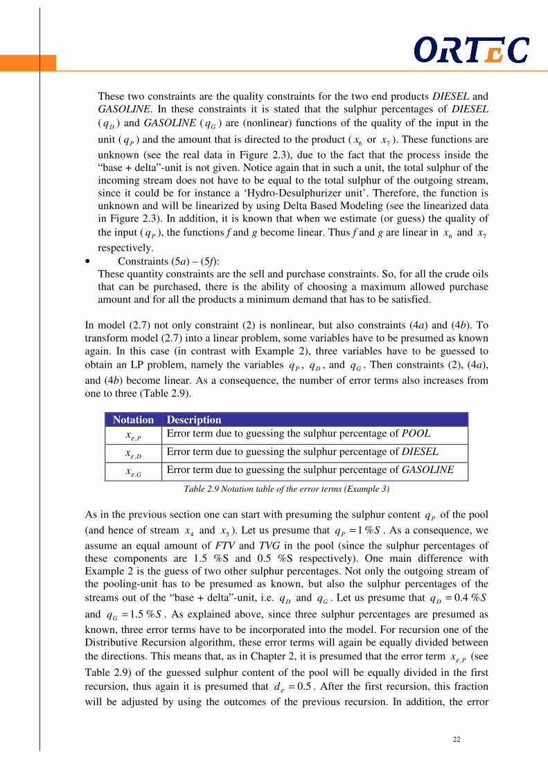
Notation Description
Px ,ε Error term due to guessing the sulphur percentage of POOL
Dx ,ε Error term due to guessing the sulphur percentage of DIESEL
Gx ,ε Error term due to guessing the sulphur percentage of GASOLINE
Table 2.9 Notation table of the error terms (Example 3)
As in the previous section one can start with presuming the sulphur content Pq of the pool
(and hence of stream 4x and 5x ). Let us presume that SqP %1= . As a consequence, we
assume an equal amount of FTV and TVG in the pool (since the sulphur percentages of these components are 1.5 %S and 0.5 %S respectively). One main difference with Example 2 is the guess of two other sulphur percentages. Not only the outgoing stream of the pooling-unit has to be presumed as known, but also the sulphur percentages of the
streams out of the “base + delta”-unit, i.e. Dq and Gq . Let us presume that SqD %4.0=
and SqG %5.1= . As explained above, since three sulphur percentages are presumed as
known, three error terms have to be incorporated into the model. For recursion one of the Distributive Recursion algorithm, these error terms will again be equally divided between
the directions. This means that, as in Chapter 2, it is presumed that the error term Px ,ε (see
Table 2.9) of the guessed sulphur content of the pool will be equally divided in the first
recursion, thus again it is presumed that 5.0=εd . After the first recursion, this fraction
will be adjusted by using the outcomes of the previous recursion. In addition, the error
23
23
terms Dx ,ε and Gx ,ε do not have to be divided into fractions, since the production of
DIESEL and GASOLINE has only one outgoing stream ( 6x and 7x respectively). The
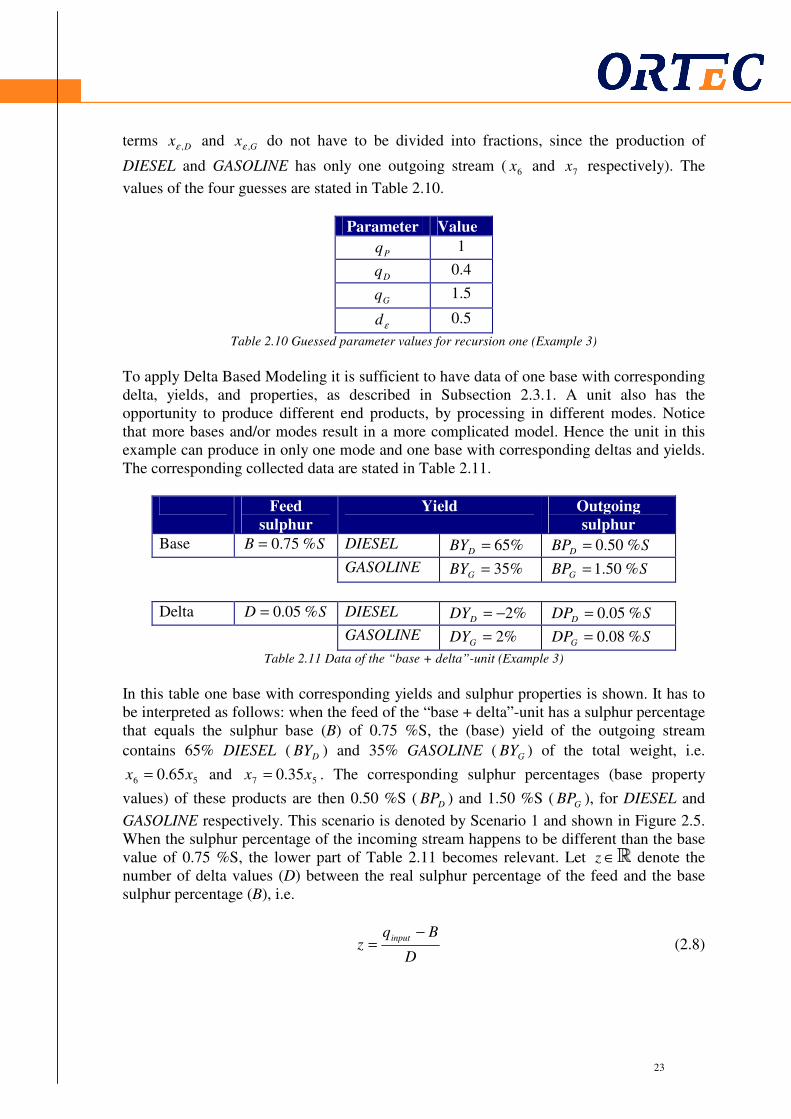
values of the four guesses are stated in Table 2.10.
Parameter Value
Pq 1
Dq 0.4
Gq 1.5
εd 0.5
Table 2.10 Guessed parameter values for recursion one (Example 3)
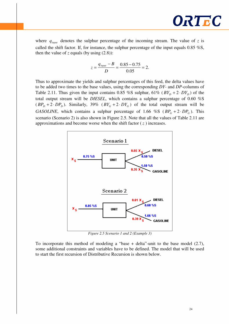
To apply Delta Based Modeling it is sufficient to have data of one base with corresponding delta, yields, and properties, as described in Subsection 2.3.1. A unit also has the opportunity to produce different end products, by processing in different modes. Notice that more bases and/or modes result in a more complicated model. Hence the unit in this example can produce in only one mode and one base with corresponding deltas and yields. The corresponding collected data are stated in Table 2.11.
Feed sulphur
Yield Outgoing sulphur
Base SB %75.0= DIESEL %65=DBY SBPD %50.0=
GASOLINE %35=GBY SBPG %50.1=
Delta SD %05.0= DIESEL %2−=DDY SDPD %05.0=
GASOLINE %2=GDY SDPG %08.0=
Table 2.11 Data of the “base + delta”-unit (Example 3)
In this table one base with corresponding yields and sulphur properties is shown. It has to be interpreted as follows: when the feed of the “base + delta”-unit has a sulphur percentage that equals the sulphur base (B) of 0.75 %S, the (base) yield of the outgoing stream
contains 65% DIESEL ( DBY ) and 35% GASOLINE ( GBY ) of the total weight, i.e.
56 65.0 xx = and 57 35.0 xx = . The corresponding sulphur percentages (base property
values) of these products are then 0.50 %S ( DBP ) and 1.50 %S ( GBP ), for DIESEL and
GASOLINE respectively. This scenario is denoted by Scenario 1 and shown in Figure 2.5. When the sulphur percentage of the incoming stream happens to be different than the base value of 0.75 %S, the lower part of Table 2.11 becomes relevant. Let ∈z denote the number of delta values (D) between the real sulphur percentage of the feed and the base sulphur percentage (B), i.e.
D
Bqz
input −= (2.8)
24
24
where inputq denotes the sulphur percentage of the incoming stream. The value of z is
called the shift factor. If, for instance, the sulphur percentage of the input equals 0.85 %S, then the value of z equals (by using (2.8)):
.205.0
75.085.0=
−=
−=
D
Bqz
input
Thus to approximate the yields and sulphur percentages of this feed, the delta values have to be added two times to the base values, using the corresponding DY- and DP-columns of
Table 2.11. Thus given the input contains 0.85 %S sulphur, 61% ( DD DYBY ⋅+ 2 ) of the
total output stream will be DIESEL, which contains a sulphur percentage of 0.60 %S
( DD DPBP ⋅+ 2 ). Similarly, 39% ( GG DYBY ⋅+ 2 ) of the total output stream will be
GASOLINE, which contains a sulphur percentage of 1.66 %S ( GG DPBP ⋅+ 2 ). This
scenario (Scenario 2) is also shown in Figure 2.5. Note that all the values of Table 2.11 are approximations and become worse when the shift factor ( z ) increases.
Figure 2.5 Scenario 1 and 2 (Example 3)
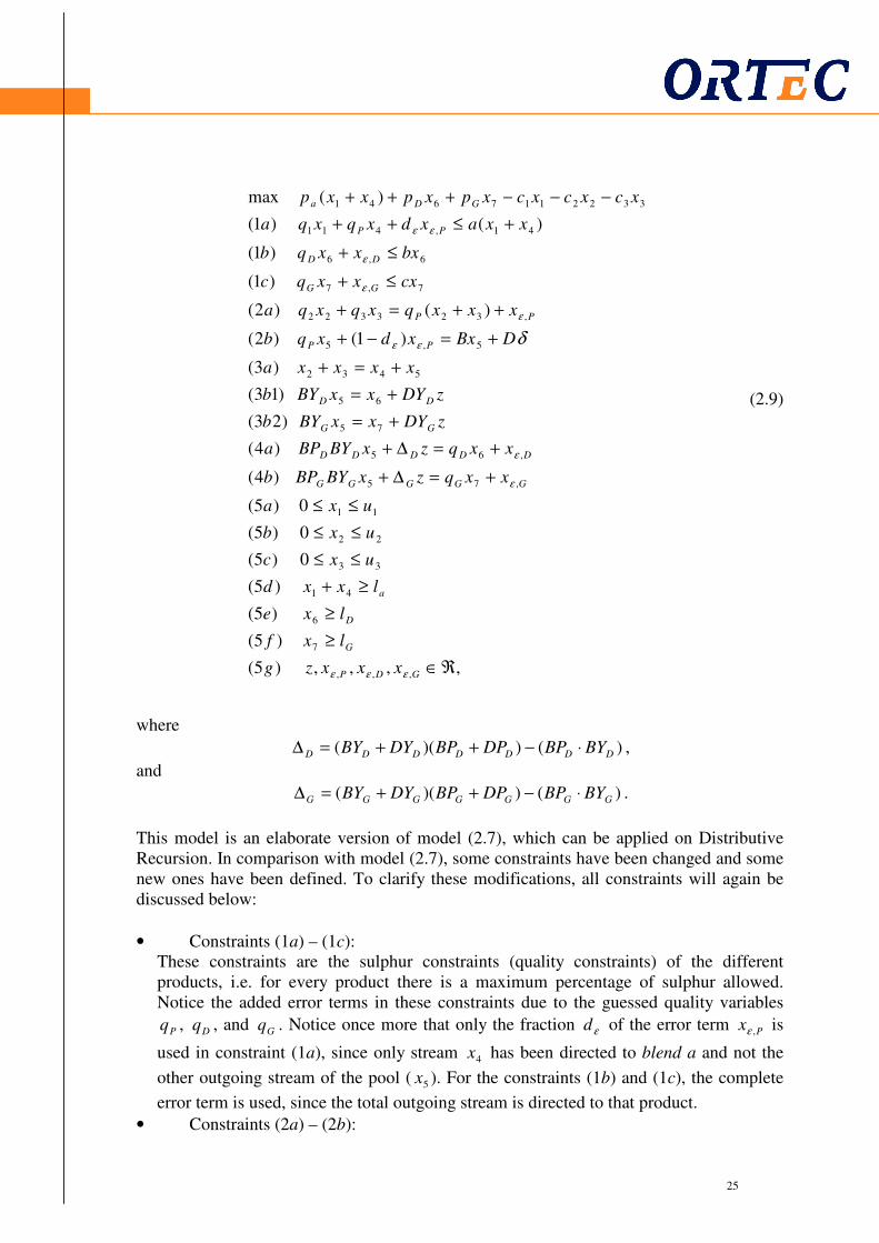
To incorporate this method of modeling a “base + delta”-unit to the base model (2.7), some additional constraints and variables have to be defined. The model that will be used to start the first recursion of Distributive Recursion is shown below.
25
25
,,,,)5(
)5(
)5(
)5(
0)5(
0)5(
0)5(
)4(
)4(
)23(
)13(
)3(
)1()2(
)()2(
)1(
)1(
)()1(
)(max
,,,
7
6
41
33
22
11
,75
,65
75
65
5432
5,5
,323322
7,7
6,6
41,411
3322117641
ℜ∈
≥
≥
≥+
≤≤
≤≤
≤≤
+=∆+
+=∆+
+=
+=
+=+
+=−+
++=+
≤+
≤+
+≤++
−−−+++
GDP
G
D
a
GGGGG
DDDDD
GG
DD
PP
PP
GG
DD
PP
GDa
xxxzg
lxf
lxe
lxxd
uxc
uxb
uxa
xxqzxBYBPb
xxqzxBYBPa
zDYxxBYb
zDYxxBYb
xxxxa
DBxxdxqb
xxxqxqxqa
cxxxqc
bxxxqb
xxaxdxqxqa
xcxcxcxpxpxxp
εεε
ε
ε
εε
ε
ε
ε
εε
δ
(2.9)
where
)())(( DDDDDDD BYBPDPBPDYBY ⋅−++=∆ ,
and
)())(( GGGGGGG BYBPDPBPDYBY ⋅−++=∆ .
This model is an elaborate version of model (2.7), which can be applied on Distributive Recursion. In comparison with model (2.7), some constraints have been changed and some new ones have been defined. To clarify these modifications, all constraints will again be discussed below:
• Constraints (1a) – (1c): These constraints are the sulphur constraints (quality constraints) of the different products, i.e. for every product there is a maximum percentage of sulphur allowed. Notice the added error terms in these constraints due to the guessed quality variables
Pq , Dq , and Gq . Notice once more that only the fraction εd of the error term Px ,ε is
used in constraint (1a), since only stream 4x has been directed to blend a and not the
other outgoing stream of the pool ( 5x ). For the constraints (1b) and (1c), the complete
error term is used, since the total outgoing stream is directed to that product.
• Constraints (2a) – (2b):
26
26
These constraints are the quality constraints for the two different units. For the unit POOL, constraint (2a) can be interpreted as the condition that the weighted sulphur percentage of the pool has to equal the guessed sulphur percentage of the outgoing
stream plus the error term Px ,ε , which is correct by definition. As explained earlier, this
error term is divided between the two directions by using the fraction εd . Constraint
(2b) is the quality constraint for UNIT. The error term Px ,ε is again partly being used
due to the guess of Pq . Thus the left hand side of the constraint is the expected sulphur
content in the stream 5x and the right hand side is the linear approximation, using the
base and delta values of Table 2.11.
• Constraint (3a): This is again the quantity constraint of the pool unit, equal to constraint (3a) of model (2.7).
• Constraints (3b1) – (3b2): These two constraints are the substitutions of constraint (3b) of model (2.7), since the outgoing stream of the unit is not known in advance when using DBM. These constraints are the quantity constraints for the two directions DIESEL and GASOLINE. In words, constraint (3b1) means for instance that the total part of the incoming streams that will be directed to DIESEL, assuming the data of the base case, has to equal the total outgoing stream directed to DIESEL, adapted with the corresponding delta values.
• Constraints (4a) – (4b): These two constraints resemble the previous two; however, one should note that these two are quality constraints whereas (3b1) and (3b2) are quantity constraints. The right
hand side of for instance constraint (4a) is the outgoing yield 6x times the
approximated sulphur percentage Dq (with corresponding error term Dx ,ε ) of the
outgoing stream. Thus the left hand side of the constraint has to contain the yield times the sulphur percentage of the incoming stream. The expected yield of the incoming
stream that will become DIESEL will be 5xBYD plus a certain term for the number of
deltas that the feed property deviates from the base value. To see this, note that %DBY
of the incoming stream in the base case flows to DIESEL. This whole term at the left hand side has to be multiplied with the base property value for DIESEL (similar to the
right sight). The extra term zD∆ is added for the number of deltas that the feed property
deviates from the base value. Notice the coefficient D∆ in front of the shift vector. This
value has been calculated with the following expression:
)())(( DDDDDDD BYBPDPBPDYBY ⋅−++=∆ ,
and equivalently for the GASOLINE case. The reason of this expression is beyond the scope of this thesis and will be assumed as given.
• Constraints (5a) – (5f): These quantity constraints are the sell and purchase constraints. Thus, for all the crude oils that can be purchased, there is the ability of choosing a maximum allowable purchase amount and for all the three products a minimum demand that has to be satisfied.
Using the values of Table 2.8, 2.10, and 2.11, model (2.9) can be filled in and simplified into the following LP problem:

27
27
ℜ∈
≥
≥
≥+
≤≤
≤≤
≤≤
=+−
=++
=−
=+
+=+
=+
+=
≤+
≤+
≤+
+++−−
GDP
G
D
P
P
G
D
P
xxxzg
xf
xe
xxd
xc
xb
xa
xxzxb
xxzxa
xzxb
xzxb
xxxxa
zxxb
xxxa
xxxc
xxxb
xxxa
xxxxxx
,,,
7
6
41
3
2
1
5,7
5,6
57
56
5432
,5
,32
7,7
6,6
4,1
764321
,,,)5(
0)5(
0)5(
100)5(
2000)5(
2000)5(
2000)5(
525.00596.05.1)4(
325.00215.04.0)4(
35.002.0)23(
65.002.0)13(
)3(
05.02125.0)2(
5.05.0)2(
5.15.1)1(
5.05.0)1(
2/15.1)1(
56232max
εεε
ε
ε
ε
ε
ε
ε
ε
(2.10)
Model (2.10) is an arbitrary LP problem and solvable with an LP-solver, such as CPlex or
Xpress, with decision variables 1x , 2x , 3x , 4x , 5x , 6x , 7x , Px ,ε , Dx ,ε , Gx ,ε , and z . On a
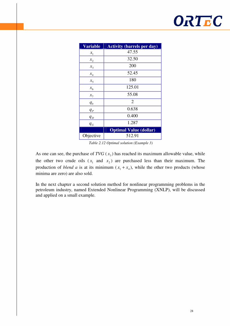
similar way as in Section 2.2, the recursion steps of Distributive Recursion can be executed. In this case, it takes four recursions to obtain a solution that proves to be a sufficiently good approximation of the optimal solution of the nonlinear problem. The final relevant activities are shown in Table 2.12.
28
28
Variable Activity (barrels per day)
1x 47.55
2x 32.50
3x 200
4x 52.45
5x 180
6x 125.01
7x 55.08
bq 2
Pq 0.638
Dq 0.400
Gq 1.287
Optimal Value (dollar)
Objective 512.91
Table 2.12 Optimal solution (Example 3)
As one can see, the purchase of TVG ( 3x ) has reached its maximum allowable value, while
the other two crude oils ( 1x and 2x ) are purchased less than their maximum. The
production of blend a is at its minimum ( 41 xx + ), while the other two products (whose
minima are zero) are also sold. In the next chapter a second solution method for nonlinear programming problems in the petroleum industry, named Extended Nonlinear Programming (XNLP), will be discussed and applied on a small example.

29
29
3 Extended Nonlinear Programming
3.1 Introduction
In this chapter Extended Nonlinear Programming (XNLP) will be discussed in a theoretical way. First the main difference with Distributive Recursion will be elaborated and after that two versions of XNLP will be discussed. The first version uses the nonlinear solver CONOPT to solve the refinery-planning problems. This method will be extensively discussed in Section 3.2 and applied on an example. The second one uses the nonlinear solver XSLP and will be briefly discussed in Section 3.3. Extended Nonlinear Programming is a new nonlinear solution method available in the PIMS software package. At this moment Shell is still using Distributive Recursion at its petroleum refineries worldwide, since they are not (yet) familiar with XNLP. The main difference between these two methods is the way of using and implementing the information from every recursion. This difference between the two solution methods is shown in Figure 3.1.
Figure 3.1 Flow diagrams of DR and XNLP
In the case of Distributive Recursion (which has extensively been explained in Chapter 2), a nonlinear programming problem is sent to PIMS where the user also has to define an initial guess (arrows 1) to transform the nonlinear problem into a linear one. Then the linear programming problem is expressed in a matrix and sent to a linear solver (like Xpress and CPlex) (arrow 2). After that it will return to PIMS (arrow 3) and will be checked whether the solution is appropriate enough. When the solution does not prove to be a sufficiently good approximation, new guesses will be chosen and a new input will be sent to the solver (arrow 4). When, after several recursions, the solution finally proves to be a sufficiently good approximation of the optimal solution of the NLP problem, the method stops and PIMS produces the “optimal” solution as the output (arrow 5).
30
30
The new solution method in PIMS, Extended Nonlinear Programming, has a different way of calculating the optimal solution, which is also shown in Figure 3.1. Again a nonlinear problem is sent to PIMS (arrow 1), together with an initial guess specified by the user. This will again be sent to the solver (arrow 2), expressed in a matrix. After that, the solver sends the first approximation back to PIMS (arrow 3). Thus until this step there is no difference between DR and XNLP. Though in this case PIMS does not send a new guess back to the linear solver, but sends the linear information as a first guess, together with the nonlinear model to a nonlinear solver (CONOPT or XSLP) (arrow 4). Inside that solver several iterations will be executed to obtain a sufficiently good solution (arrow 5). After that, it will be returned to PIMS (arrow 6), where the output will be accessible for the user (arrow 7). Thus, the recursion steps are now executed outside PIMS and inside the nonlinear solver. The working of the two different nonlinear solvers will be discussed in the rest of this chapter.
3.2 The CONOPT solver
One of the available solvers for the XNLP method is CONOPT. CONOPT is a commercial solver used in software packages such as AIMMS, Matlab, and PIMS. This solver uses the Generalized Reduced Gradient (GRG) method to solve the (nonlinear) problems, which is described by de Klerk et al. (2005). The GRG method is a generalization of the reduced gradient method. The Reduced Gradient method was developed by Wolfe (1963) to solve a nonlinear problem with linear constraints. The basic idea of this Reduced Gradient method is that under certain assumptions all variables can be expressed in terms of an independent subset of the variables. Hence the number of variables in the model will be reduced to approximate the optimal solution. The Generalized Reduced Gradient method can also be applied on nonlinear problems with nonlinear constraints. The basic idea of the GRG method, which has been developed by Abadie and Carpentier (1969), is to replace the nonlinear constraints by their linear Taylor approximation at the current value of x, and then apply the reduced gradient method. Hence the Generalized Reduced Gradient method has basically the same structure as the Reduced Gradient method. Since the nonlinear problems at the refineries contain several nonlinear constraints, the generalized version of the method is used in PIMS and will be discussed below, based on de Klerk et al. (2005).
3.2.1 GRG method
First let us assume that the problem at the refinery can be written as:
(3.1)
where the functions mhhf ,,, 1 L are supposed to be continuously differentiable. To
illustrate this method with an example, the method will first be explained in general. Therefore some notation and assumptions are required.
,0
,,1,0)(..
)(min
≥
==
x
mjxhts
xf
j L
31
31
Let us assume that the gradients of the constraint functions mhh ,,1 L are linearly
independent at every point 0≥x and that each feasible value of x has at least m positive components. Let F denote all values of x for which the problem has been solved. Note that when the constraints are nonlinear, the feasible region F may not be convex. This could cause extra effort, which could result in executing more iterations before a sufficiently good solution has been found.
In the initialization step of the method ( 0=t ), a feasible solution 00 ≥=tx with
0)( 0 ==tj xh for all j has to be chosen. This solution is usually equal to the first solution
obtained in Distributive Recursion (as shown in Figure 3.1). The vector x can be divided
into a basic Bx and a non-basic part Nx , i.e. ),( | itNiB|tit xxx === = for 0≥i . Note that in first
case the choice of itBx =| is restricted to nonnegative values. Furthermore, the Jacobian
matrix of the constraints T
m xhxhxH ))(,),(()( 1 L= at each 0≥x is denoted by )(xJH
and has full rank. Consequently, the matrix )(xJH can also be divided into a basic part B
and a non-basic part N, i.e. )()( NBxJH = with the Bx -columns stated in part B and the
Nx -columns in part N.
Now the constraints TxH 0)( = can be linearized by the first-order Taylor approximation1,
using the Jacobian matrix:
.0))(())(()()( 00000
T
ttttt xxxJHxxxJHxHxH =−=−+≈ =====
To see this, note that T
txH 0)( 0 == . Using this equation, the following expression can be
derived:
NBtt NxBxxxJH +=== 00 )( . (3.2)
To see this, note that the matrix )(xJH and the vector x both have been divided into two
parts: the basic and non-basic part. Hence, multiplying the matrix )(xJH with the vector x
results in a summation of both products as shown in (3.2). This equation can now be
simplified, by denoting the left hand side of the expression by b, so 00 )( === tt xxJHb .
Then by using equation (3.2), the variables in the basis B can be written as
NB NxBbBx 11 −− −= . (3.3)
Using this expression, model (3.1) can be written as
(3.4)
1 In general the first-order Taylor expansion for a function f(x) in a point x is defined by
))(()()( xxxfxfxf −∇+≈ , where )(xf∇ denotes the gradient of the function in x .
,0
0..
)(min
11
≥
≥−= −−
N
NB
NN
x
NxBbBxts
xf
32
32
where ),()( 11
NNNN xNxBbBfxf −− −= . To see this, note that the constraints TxH 0)( =
of model (3.1) are now substituted by expression (3.3), which results in a model without restrictions (except the non-negativity constraints). Thus the objective function of model (3.4) has to be minimized, taking into account that the variables stay positive. After these steps, the method continues with calculating the search directions for the basic and non-basic variables by using the steepest descent method. The steepest descent method is a line search method that moves in the opposite direction than the derivative of the objective function. This is the most obvious choice for a search direction, since the objective value will always decrease maximally when x increases with a sufficiently small
0>ε . Thus the search direction of the nonbasic variable is defined as
(3.5a)
Converting ),()( 11
NNNN xNxBbBfxf −− −= into a function of Bx results in
),()( 11
BBBB BxNbNxfxf −− −= . Now the search direction of the basic variables can be
written as
Now by using the chain rule2 this becomes
(3.5b)
These search directions are necessary to determine the new values for Nx and Bx . One
uses the formulas
N
OLD
N
NEW
N sxx λ+= , (3.6a)
(3.6b)
for the non-basic and basic variables respectively. Let ∗λ denote the value of λ for which the objective function of model (3.4) has been minimized (without taking into account the nonnegativity constraints). This can be done by filling in expression (3.6a) in the objective
function of (3.4) and optimizing this function with respect to λ . Let maxλ denote the
maximum absolute value of λ for which both variables are still nonnegative (by using
(3.6)). Now the optimal value of λ equals ∗λ when maxλλ ≤∗ , and maxλ when maxλλ >∗ .
With this optimal value of λ , the new values of Nx and Bx can be calculated by using
2 If )(xfy = and )(tgx = then dt
dx
dx
dy
dt
dy= .
.))(()(
B
BNB
B
BBB
x
xxf
x
xfs
δ
δ
δ
δ−=−=
,B
OLD
B
NEW
B sxx λ+=
.)()( 11
N
N
NNB NsBNB
x
xfs −− −=⋅
−⋅−−=
δ
δ
.)(
N
NNN
x
xfs
δ
δ−=
33
33
expressions (3.6). After that, these new values have to be checked for feasibility by using model (3.1). When they are not feasible, the basic variable usually has to be adjusted and the whole procedure has to be repeated with these values, until a good solution has been found. The steps that have to be followed for executing the GRG method for a given nonlinear model with nonlinear constraints of the form as model (3.1) are summarized below. Initialization:
• Start with iteration i=0.
• Find a feasible solution itx = and divide this solution into a basic ( Bx ) and a non-
basic ( Nx ) part.
• Define a stopping value 0>ε such that the algorithm stops when ε<)(xH .
Step 1:
• Calculate the Jacobian A and corresponding vector b by using
and
itAxb == .
The matrix A will now be divided into a set of columns N and a set of columns B. The columns in N are the columns that are differentiated with respect to a non-basic variable and the columns in B are those that are differentiated with respect to a basic variable.
Step 2:
• Write Bx as a function of Nx by using equation (3.3).
Step 3:
• Rewrite the starting model into a model similar as (3.4), with only non-basic variables by using the obtained expression(s) in Step 2.
Step 4:
• Determine the search directions, using equations (3.5a) and (3.5b). Step 5:
• Determine the solutions for the next iteration, using iNiNiN sxx ||1| λ+=+
and iBiBiB sxx ||1| λ+=+ .
Step 6:
• Calculate the maximum allowable value maxλ of λ , such that 1| +iNx and 1| +iBx are
still nonnegative.
),( itxJHA ==

34
34
• Calculate the value ∗λ that optimizes the objective function of model (3.4) (without taking into account the nonnegativity constraints).
• If maxλλ ≤∗ , then ∗+ = λλ 1i .
If maxλλ >∗ , then max1 λλ =+i .
Step 7:
• Fill in 1+iλ in the equations of Step 5 and calculate 1| +iBx and 1| +iNx by using the
equations of Step 5. Step 8:
• While ε≥+= )( 1itxH , adapt 1| +iBx such that 0)( 1 =+=itxH , i=i+1 and start again at
Step 1. When elements of 1| +iBx are positive, those variables will remain as basic
ones. Otherwise, new basic variables have to be chosen for the next iteration. The non-basic variable with the largest absolute value of gradient is selected to enter the basic variable set, according to Lee et al. (2004).
• When ε<+= )( 1itxH , the vector 1+=itx has to be adjusted in the same way as above
(to deal with the constraints). This vector is the optimal solution with corresponding objective function value.
3.2.2 GRG method applied on an NLP problem (Example 4)
To illustrate the GRG method with an example, we apply it on the following nonlinear programming problem:
(3.7)
Iteration 1:
Initialization: Let us start from the point TT
ttt xxx )42()( 0|20|10 == === with an objective
value of 68 and let us assume that for this recursion, 2x is the basic variable. Let us also
define the stop value: 16.0=ε . Step 1: The Jacobian matrix of the constraints equals:
( ) ( ) ( )16442)( 0|20|1
2
1
1
10 ==
∂
∂
∂
∂=== === ttt xx
x
h
x
hBNxJHA .
From this, we get
( ) 724
21640 =
== =tAxb .
Step 2: Now by using equation (3.3), this basic variable can be written as a function of the non-basic variable:
.0,
0362..
242min
21
2
2
2
1
1
2
2
2
1
≥
=−+
−+
xx
xxts
xxx
35
35
111
11
2 25.05.4416
172
16
1xxNxBbBx −=−=−= −− .
Step 3: Hence the objective function becomes
)25.05.4,(),()( 111
11
111 xxfNxBbBxfxf −=−= −− .
Using this objective function, model (3.4) can be written as
This equals
(3.8)
Hence this model can now be optimized by solving this model, i.e. minimizing this
objective function, taking into account the nonlinearity of the variable 1x and indirectly of
2x .
Step 4: Now the search directions of the basic and the non-basic variable, denoted by Bs
and Ns respectively, have to be determined:
,2115.4)(
0|1
1
0|1
0|10| =+−=−== =
=
== t
tN
ttN xx
xfss
δ
δ
and
Step 5: Thus now the new variables can be calculated by using the search directions determined above.
0220|0|11|1 ≥+=+= === λλ tNtt sxx , (3.9a)
05.040|0|21|2 ≥−=+= === λλ tBtt sxx . (3.9b)
.0
025.05.4..
2)25.05.4(42min
1
1
1
2
1
2
1
≥
≥−
−−+
x
xts
xxx
.0
025.05.4..
181125.2min
1
1
1
2
1
≥
≥−
+−
x
xts
xx
.5.02416
10|
1
0|20| −=⋅−=−== =−
== tNttB NsBss

36
36
Step 6: Using expressions (3.9), one can arrive that 8max =λ , because larger values result
in a negative value for 1|2 =tx . Now using formulas (3.9), the objective function of model
(3.8) can be rewritten into:
181125.2min 1|1
2
1|1 +− == tt xx .
In terms of λ it becomes
549min 2 +− λλ .
This objective function can now be minimized with respect to λ , by solving the equation
( ) 0549 2 =+− λλδλ
δ.
This results in the following optimal value of ∗λ :
11022.2 −∗ ⋅=λ .
Since maxλλ <∗ the optimal value of λ now equals 1
1 1022.2 −⋅=λ .
Step 7: Inserting this value of λ into expressions (3.9), results in
TT
ttt xxx )889.3444.2()( 1|21|11 == === .
Step 8: As expected, the constraint of model (3.8) (and thus of model (3.7)) will not hold when using these values. This is due to the nonlinearity of the constraint. Since
ε>== 222.0)( 1txH , the basic variable 2x will be adjusted such that the constraints of the
original model (3.7) hold, i.e. TT
ttt xxx )875.3444.2()( 1|21|11 == === with an objective
value of 111.67 . Consequently, only Bx changes and 1xxN = stays fixed. These
(feasible) values of x are the starting points for the next iteration, which will be similar to
Iteration 1. Now 2x will again be the basic variable, since 1|1 =tx stayed positive. All
iteration steps, necessary to obtain a sufficiently good solution, are similar to the one above and hence elaborated in Appendix B. The final solution of the GRG method for this example has been obtained after 5 iterations. This optimal solution has an objective function value of 64.162 with a corresponding optimal value of x:
T
tx )211.3922.3(5 == .
The method explained in this section is used in the solver CONOPT in the XNLP mode and has a structure that differs significantly from the solution method used in Distributive Recursion. In the next section, the second solver available in the XNLP mode will be described.

37
37
3.3 The XSLP solver
XSLP is a solver developed by AspenTech (developers of PIMS) and based on the sequential or successive linear programming (SLP) method. This method is about solving a nonlinear programming problem by a sequence of linear approximations and by using linear programming to solve each subproblem, as explained by Pike (2001). These subproblems are problems in which the constraints and objective function of the original model are linearized by using the first-order Taylor expansion. Notice that the linear solution method Distributive Recursion (Chapter 2) is also a variant of the SLP method, but significantly differs from this nonlinear solver (as will be clear in this section). Let us assume that the nonlinear problem of the refinery is again of the following structure:
(3.10)
where the functions mhhf ,,, 1 L are supposed to be continuously differentiable and may
be nonlinear. This model can be linearized around a feasible point kx at each iteration k,
using the Taylor expansion as defined in Section 3.2. This means that the nonlinear constraint functions in the subproblems can be locally approximated by
mjxxxhxhxh kkjkjj ,,1))(()()( L=−∇+≈ .
The objective function of the subproblem will be linearized in the same manner as the
constraints. However, the first term at the right hand side )( kxf will be removed; since it
is a constant in the objective function, it does not influence the optimal value of x. However, note that it does influence the objective function value, but since we are interested in the optimal value of x for each subproblem, it is not significant for that computation. Using these linearizations, the subproblem of model (3.10) becomes
This can be rewritten in the form
(3.11)
This submodel can now be solved with an LP algorithm, using )( kxx − as the decision
variable, such as the Simplex algorithm. However, since the Simplex algorithm usually
works with non-negative variables and since the values of )( kxx − can take on both
positive and negative values (depending on the location of the optimum), a change of
,0
,,10)(..
)(min
≥
==
x
mjxhts
xf
j L
.0
,,10))(()(..
))((min
≥
==−∇+
−∇
x
mjxxxhxhts
xxxf
kkjkj
kk
L
.0
,,1)())((..
))((min
≥
=−=−∇
−∇
x
mjxhxxxhts
xxxf
kjkkj
kk
L
38
38
variables has to be done. Griffith & Stewart (1961) introduced the following substitution to deal with this issue:
−+ −−−=− )()()( kkk xxxxxx , (3.12)
where
.0)(
0)(
0
)()(
,0)(
0)(
0
)()(
>−
≤−
−−
=−
<−
≥−
−
=−
−
+
k
kk
k
k
kk
k
xxif
xxifxxxx
xxif
xxifxxxx
Substituting equation (3.12) into model (3.11) results in the following linear problem, which can be solved using the Simplex algorithm:
(3.13)
After this problem has been solved, it will be checked whether or not the corresponding value of x is a sufficiently good approximation of the optimal solution of the original model (3.10) and it will be decided whether or not a new iteration will be started with the
current value of x as new starting point 1+kx . We omit the details of how these can be
done. Finally, note that the feasible starting point for the first recursion can be obtained by running the first recursion of the Distributive Recursion algorithm. Besides CONOPT and XSLP there are other appropriate nonlinear solvers available on the market, such as SNOPT and MINOS. These packages for solving nonlinear programming problems are not available in PIMS, but to give a good overview and to compare the solvers described above with other ones, they will be briefly discussed and compared in the next chapter.
.)()(
,,1)())(())((..
))(())((min
kkk
kjkkjkkj
kkkk
xxxxx
mjxhxxxhxxxhts
xxxfxxxf
−≥−−−
=−=−∇−−∇
−∇−−∇
−+
−+
−+
L
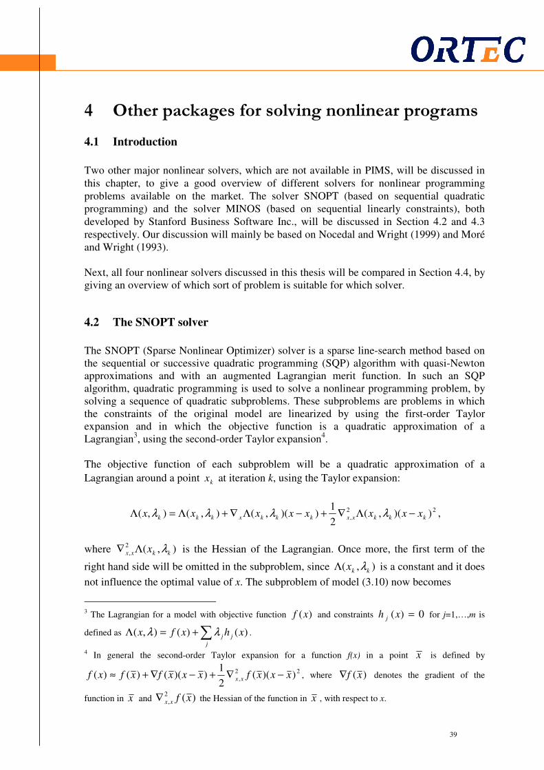
39
39
4 Other packages for solving nonlinear programs
4.1 Introduction
Two other major nonlinear solvers, which are not available in PIMS, will be discussed in this chapter, to give a good overview of different solvers for nonlinear programming problems available on the market. The solver SNOPT (based on sequential quadratic programming) and the solver MINOS (based on sequential linearly constraints), both developed by Stanford Business Software Inc., will be discussed in Section 4.2 and 4.3 respectively. Our discussion will mainly be based on Nocedal and Wright (1999) and Moré and Wright (1993). Next, all four nonlinear solvers discussed in this thesis will be compared in Section 4.4, by giving an overview of which sort of problem is suitable for which solver.
4.2 The SNOPT solver
The SNOPT (Sparse Nonlinear Optimizer) solver is a sparse line-search method based on the sequential or successive quadratic programming (SQP) algorithm with quasi-Newton approximations and with an augmented Lagrangian merit function. In such an SQP algorithm, quadratic programming is used to solve a nonlinear programming problem, by solving a sequence of quadratic subproblems. These subproblems are problems in which the constraints of the original model are linearized by using the first-order Taylor expansion and in which the objective function is a quadratic approximation of a Lagrangian3, using the second-order Taylor expansion4. The objective function of each subproblem will be a quadratic approximation of a
Lagrangian around a point kx at iteration k, using the Taylor expansion:
22
, ))(,(2
1))(,(),(),( kkkxxkkkxkkk xxxxxxxx −Λ∇+−Λ∇+Λ=Λ λλλλ ,
where ),(2
, kkxx x λΛ∇ is the Hessian of the Lagrangian. Once more, the first term of the
right hand side will be omitted in the subproblem, since ),( kkx λΛ is a constant and it does
not influence the optimal value of x. The subproblem of model (3.10) now becomes
3 The Lagrangian for a model with objective function )(xf and constraints 0)( =xh j for j=1,…,m is
defined as )()(),( xhxfxj
jj∑+=Λ λλ .
4 In general the second-order Taylor expansion for a function f(x) in a point x is defined by
22
, ))((2
1))(()()( xxxfxxxfxfxf xx −∇+−∇+≈ , where )(xf∇ denotes the gradient of the
function in x and )(2
, xfxx∇ the Hessian of the function in x , with respect to x.

40
40
.0
,,10))(()()(..
))(,(2
1))(,(min 22
,
≥
==−∇+≈
−Λ∇+−Λ∇
x
mjxxxhxhxhts
xxxxxx
kkjkjj
kkkxxkkkxx
L
λλ
(4.1)
The sequential QP approach outlined above requires the computation of ),(2
, kkxx x λΛ∇ at
iteration k. Most of the SQP methods (including SNOPT) use the quasi-Newton approximation of this Hessian, i.e. it replaces this matrix with the Broyden-Fletcher-
Goldfarb-Shanno (BFGS) approximation kB . This approximation is defined as
),( 11
2
,1 λxB xx Λ∇= ,
and for iteration 1>k
k
T
k
T
kk
kk
T
k
k
T
kkkkk
sy
yy
sBs
BssBBB +−=+1 ,
where kkk xxs −= +1 and ),(),( 1 kkxkkxk xxy λλ Λ∇−Λ∇= + . Explaining why such an
approximation is suitable for these problems is beyond the scope of this thesis. Solving the QP subproblem (4.1) with approximated Hessian is itself an iterative procedure. Again, the details of how this iterative procedure is carried out are beyond the scope of this thesis. After the QP subproblem has been solved, the next step is to choose a new starting point
for the next iteration, i.e. 1+kx . This point will be obtained by using )(1 kkkk xxxx −+=+ α
and should not only decrease the objective value, but also move towards satisfying the
constraints. Since kx and x are already given, one only has to determine the distance kα to
move along the direction kxx − . Therefore we first have to define a merit function l ,
which determines whether or not a certain point is better than another. This function l (called Augmented Lagrangian) is defined as
{ } { }
)(2
1)()();,(
,..,1
2
,..,1
xhxhxfxmj
jj
mj
jj ∑∑∈∈
++= νλνλl , (4.2)
where ν is a vector of positive penalty parameters. Relative large values for the penalty parameters mean large weights assigned to constraint satisfaction relative to minimization
of the objective. Given the starting point kx , the search direction obtained by solving the
kth QP subproblem kxx − , and the corresponding Lagrange multipliers kλ and 1+kλ , the
optimal step length ∗kα at iteration k is now found by (approximately) minimizing
));(),(( 1 νλλαλα kkkkkkk xxx −+−+ +l .

41
41
Note that the computation of 1+kλ can be done in several ways, but to avoid the details of
this solver, these computations are beyond the scope of this thesis, but elaborated in Nocedal en Wright (1999). The optimal step length can now be used to determine the new
starting point, 1+kx . After that, one needs to check whether this value is an appropriate
solution of the original problem (3.10). The value is tested on certain tolerances that are specified by the user in advance. If this new starting point proves to be a good approximation of the optimal solution (i.e. no tolerances are violated) the solver is
finished. Otherwise, a new iteration can be executed with starting point 1+kx .
4.3 The MINOS solver
The MINOS (Modular In core Nonlinear Optimization System) solver is based on a sequential linearly constrained (SLC) method. The principal idea is not to simply use a merit function as a test of suitability for steps (as (4.2) is used), but to optimize the merit function directly. Thus this method generates a step by minimizing a Lagrangian subject to linearizations of the constraints. That means again that the constraints will be linearized, using the first-order Taylor expansion. In contrast with an SQP solver that minimizes a quadratic approximation of the original objective function subject to linear constraints (such as SNOPT), the subproblem in SLC methods optimizes a nonlinear approximation of the Lagrangian. Note that MINOS only uses an SLC method when the constraints of the problem are nonlinear (which is indeed the case in the petroleum industry). The discussion below is based on Nocedal and Wright (1999). Let us again consider the equality-constrained problem (3.10). At iteration k the subproblem with linearized constraints becomes
(4.3)
where the objective function )(xFk is defined differently for different SLC solvers that are
available on the market. To define these different objective functions, let us first denote the
difference between )(xh j and its linearization at kx by )(xh k
j∆ for every constraint j, i.e.
mjxxxhxhxhxh k
T
kjkjj
k
j ,...,1)()()()()( =−∇−−=∆ ,
at iteration k. Now the objective function )(xFk is in some of the SLC solvers, especially
the first generation SLC solvers that were available on the market, defined as
mjxhxfxFj
k
j
k
jk ,...,1)()()( =∆−= ∑λ ,
where kλ is the current Lagrange multiplier estimate. In addition, the MINOS solver adds
an extra term to the Lagrangian. In the MINOS solver )(xFk has been defined as
,0
,,10)()()(..
)(min
≥
==−∇+
x
mjxxxhxhts
xF
k
T
kjkj
kx
L
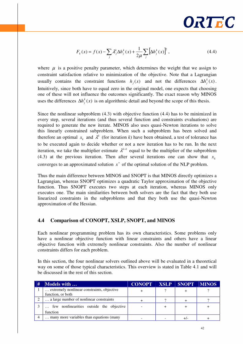
42
42
[ ]∑∑ ∆+∆−=j
k
j
j
k
j
k
jk xhxhxfxF2
)(2
1)()()(
µλ , (4.4)
where µ is a positive penalty parameter, which determines the weight that we assign to
constraint satisfaction relative to minimization of the objective. Note that a Lagrangian
usually contains the constraint functions )(xh j and not the differences )(xh k
j∆ .
Intuitively, since both have to equal zero in the original model, one expects that choosing one of these will not influence the outcomes significantly. The exact reason why MINOS
uses the differences )(xh k
j∆ is on algorithmic detail and beyond the scope of this thesis.
Since the nonlinear subproblem (4.3) with objective function (4.4) has to be minimized in every step, several iterations (and thus several function and constraints evaluations) are required to generate the new iterate. MINOS also uses quasi-Newton iterations to solve this linearly constrained subproblem. When such a subproblem has been solved and
therefore an optimal kx and kλ (for iteration k) have been obtained, a test of tolerance has
to be executed again to decide whether or not a new iteration has to be run. In the next
iteration, we take the multiplier estimate 1+kλ equal to be the multiplier of the subproblem
(4.3) at the previous iteration. Then after several iterations one can show that kx
converges to an approximated solution ∗x of the optimal solution of the NLP problem. Thus the main difference between MINOS and SNOPT is that MINOS directly optimizes a Lagrangian, whereas SNOPT optimizes a quadratic Taylor approximation of the objective function. Thus SNOPT executes two steps at each iteration, whereas MINOS only executes one. The main similarities between both solvers are the fact that they both use linearized constraints in the subproblems and that they both use the quasi-Newton approximation of the Hessian.
4.4 Comparison of CONOPT, XSLP, SNOPT, and MINOS
Each nonlinear programming problem has its own characteristics. Some problems only have a nonlinear objective function with linear constraints and others have a linear objective function with extremely nonlinear constraints. Also the number of nonlinear constraints differs for each problem. In this section, the four nonlinear solvers outlined above will be evaluated in a theoretical way on some of those typical characteristics. This overview is stated in Table 4.1 and will be discussed in the rest of this section.
# Models with … CONOPT XSLP SNOPT MINOS 1 … extremely nonlinear constraints, objective
function, or both + ? + ?
2 … a large number of nonlinear constraints + ? + ?
3 … few nonlinearities outside the objective
function
- + + +
4 … many more variables than equations (many degrees of freedom)
- - +/- +
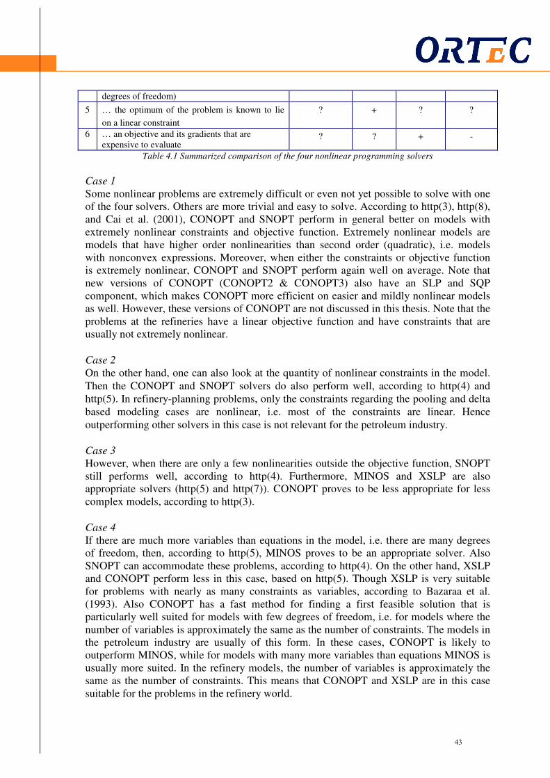
43
43
degrees of freedom)
5 … the optimum of the problem is known to lie
on a linear constraint
? + ? ?
6 … an objective and its gradients that are expensive to evaluate
? ? + -
Table 4.1 Summarized comparison of the four nonlinear programming solvers
Case 1 Some nonlinear problems are extremely difficult or even not yet possible to solve with one of the four solvers. Others are more trivial and easy to solve. According to http(3), http(8), and Cai et al. (2001), CONOPT and SNOPT perform in general better on models with extremely nonlinear constraints and objective function. Extremely nonlinear models are models that have higher order nonlinearities than second order (quadratic), i.e. models with nonconvex expressions. Moreover, when either the constraints or objective function is extremely nonlinear, CONOPT and SNOPT perform again well on average. Note that new versions of CONOPT (CONOPT2 & CONOPT3) also have an SLP and SQP component, which makes CONOPT more efficient on easier and mildly nonlinear models as well. However, these versions of CONOPT are not discussed in this thesis. Note that the problems at the refineries have a linear objective function and have constraints that are usually not extremely nonlinear. Case 2 On the other hand, one can also look at the quantity of nonlinear constraints in the model. Then the CONOPT and SNOPT solvers do also perform well, according to http(4) and http(5). In refinery-planning problems, only the constraints regarding the pooling and delta based modeling cases are nonlinear, i.e. most of the constraints are linear. Hence outperforming other solvers in this case is not relevant for the petroleum industry. Case 3 However, when there are only a few nonlinearities outside the objective function, SNOPT still performs well, according to http(4). Furthermore, MINOS and XSLP are also appropriate solvers (http(5) and http(7)). CONOPT proves to be less appropriate for less complex models, according to http(3). Case 4 If there are much more variables than equations in the model, i.e. there are many degrees of freedom, then, according to http(5), MINOS proves to be an appropriate solver. Also SNOPT can accommodate these problems, according to http(4). On the other hand, XSLP and CONOPT perform less in this case, based on http(5). Though XSLP is very suitable for problems with nearly as many constraints as variables, according to Bazaraa et al. (1993). Also CONOPT has a fast method for finding a first feasible solution that is particularly well suited for models with few degrees of freedom, i.e. for models where the number of variables is approximately the same as the number of constraints. The models in the petroleum industry are usually of this form. In these cases, CONOPT is likely to outperform MINOS, while for models with many more variables than equations MINOS is usually more suited. In the refinery models, the number of variables is approximately the same as the number of constraints. This means that CONOPT and XSLP are in this case suitable for the problems in the refinery world.
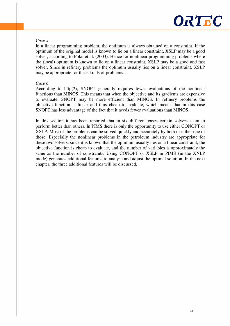
44
44
Case 5 In a linear programming problem, the optimum is always obtained on a constraint. If the optimum of the original model is known to lie on a linear constraint, XSLP may be a good solver, according to Poku et al. (2003). Hence for nonlinear programming problems where the (local) optimum is known to lie on a linear constraint, XSLP may be a good and fast solver. Since in refinery problems the optimum usually lies on a linear constraint, XSLP may be appropriate for these kinds of problems. Case 6 According to http(2), SNOPT generally requires fewer evaluations of the nonlinear functions than MINOS. This means that when the objective and its gradients are expensive to evaluate, SNOPT may be more efficient than MINOS. In refinery problems the objective function is linear and thus cheap to evaluate, which means that in this case SNOPT has less advantage of the fact that it needs fewer evaluations than MINOS.
In this section it has been reported that in six different cases certain solvers seem to perform better than others. In PIMS there is only the opportunity to use either CONOPT or XSLP. Most of the problems can be solved quickly and accurately by both or either one of those. Especially the nonlinear problems in the petroleum industry are appropriate for these two solvers, since it is known that the optimum usually lies on a linear constraint, the objective function is cheap to evaluate, and the number of variables is approximately the same as the number of constraints. Using CONOPT or XSLP in PIMS (in the XNLP mode) generates additional features to analyse and adjust the optimal solution. In the next chapter, the three additional features will be discussed.
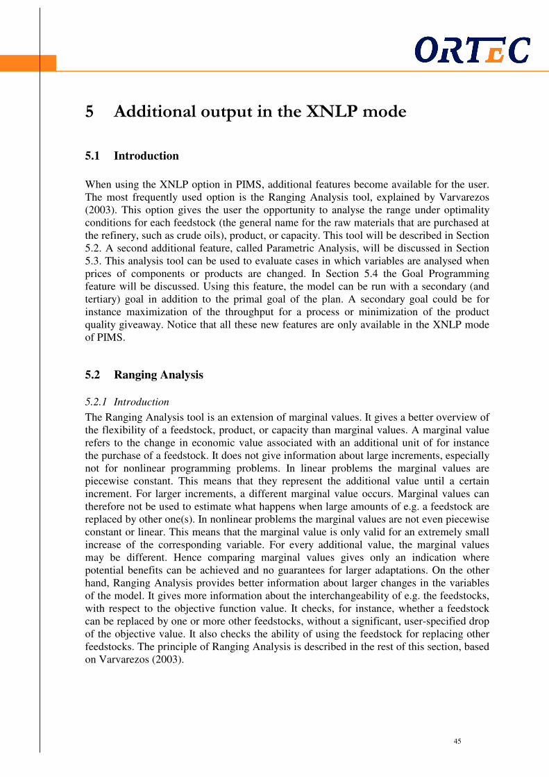
45
45
5 Additional output in the XNLP mode
5.1 Introduction
When using the XNLP option in PIMS, additional features become available for the user. The most frequently used option is the Ranging Analysis tool, explained by Varvarezos (2003). This option gives the user the opportunity to analyse the range under optimality conditions for each feedstock (the general name for the raw materials that are purchased at the refinery, such as crude oils), product, or capacity. This tool will be described in Section 5.2. A second additional feature, called Parametric Analysis, will be discussed in Section 5.3. This analysis tool can be used to evaluate cases in which variables are analysed when prices of components or products are changed. In Section 5.4 the Goal Programming feature will be discussed. Using this feature, the model can be run with a secondary (and tertiary) goal in addition to the primal goal of the plan. A secondary goal could be for instance maximization of the throughput for a process or minimization of the product quality giveaway. Notice that all these new features are only available in the XNLP mode of PIMS.
5.2 Ranging Analysis
5.2.1 Introduction
The Ranging Analysis tool is an extension of marginal values. It gives a better overview of the flexibility of a feedstock, product, or capacity than marginal values. A marginal value refers to the change in economic value associated with an additional unit of for instance the purchase of a feedstock. It does not give information about large increments, especially not for nonlinear programming problems. In linear problems the marginal values are piecewise constant. This means that they represent the additional value until a certain increment. For larger increments, a different marginal value occurs. Marginal values can therefore not be used to estimate what happens when large amounts of e.g. a feedstock are replaced by other one(s). In nonlinear problems the marginal values are not even piecewise constant or linear. This means that the marginal value is only valid for an extremely small increase of the corresponding variable. For every additional value, the marginal values may be different. Hence comparing marginal values gives only an indication where potential benefits can be achieved and no guarantees for larger adaptations. On the other hand, Ranging Analysis provides better information about larger changes in the variables of the model. It gives more information about the interchangeability of e.g. the feedstocks, with respect to the objective function value. It checks, for instance, whether a feedstock can be replaced by one or more other feedstocks, without a significant, user-specified drop of the objective value. It also checks the ability of using the feedstock for replacing other feedstocks. The principle of Ranging Analysis is described in the rest of this section, based on Varvarezos (2003).

46
46
Let us first assume that the nonlinear programming model that will be discussed in this section is of the form
(5.1)
where the only differences with model (3.10) are the explicit lower and upper bounds on
the variables, denoted by Lx and Ux respectively. To perform Ranging Analysis the so-called utility and flexibility indices are necessary. The utility index of a certain feedstock is the fraction of the remaining total feed that this particular feedstock can displace for a predefined marginal drop in the objective value. The formula for this fraction equals
,1 BASE
BASEMAX
X
XXIndexUtility
−
−= (5.2)
where BASEX is the fraction of the total feed that this feedstock represents at the base
optimal solution and MAXX is the maximum fraction of the total feed that this feedstock
can reach at near optimal conditions. The fraction BASEX can be computed by solving
model (5.1) and calculating the fraction for each crude oil. Let us denote the component of
the vector x that corresponds to the feedstock F that is analysed by Fx . The fraction MAXX
can be computed by solving the following nonlinear problem:
(5.3)
where Mε is a user-defined constant that represents the marginal relaxation of the
objective value for the Ranging Analysis and )1.5(f the optimal objective function value of
model (5.1). Thus the purchase amount of the analysed feedstock is maximized, such that the objective value is still larger than the base solution multiplied with a constant close to one. A utility index equal to zero means that the corresponding feedstock, product, or capacity cannot displace other ones within a predefined marginal drop in the objective value. This
means that, according to (5.2), MAXBASE XX = . When for instance (a part of) a certain
feedstock cannot be delivered, it cannot be displaced by other feedstocks with a utility index of zero. A utility index of one means that it can displace the whole remaining total feed and still keeps the objective value above a predefined level. Usually there are no feedstocks that have a utility index of one. If a feedstock has a relatively high utility index, it means that it can displace a high fraction of the total feed, with the objective function value not lower than a predefined level.
,
,,10)(..
)(min
UL
j
xxx
mjxhts
xf
≤≤
== L
,
)1()(
,,10)(..
max
)1.5(
UL
M
j
Fx
xxx
fxf
mjxhts
xF
≤≤
−⋅≥
==
ε
L
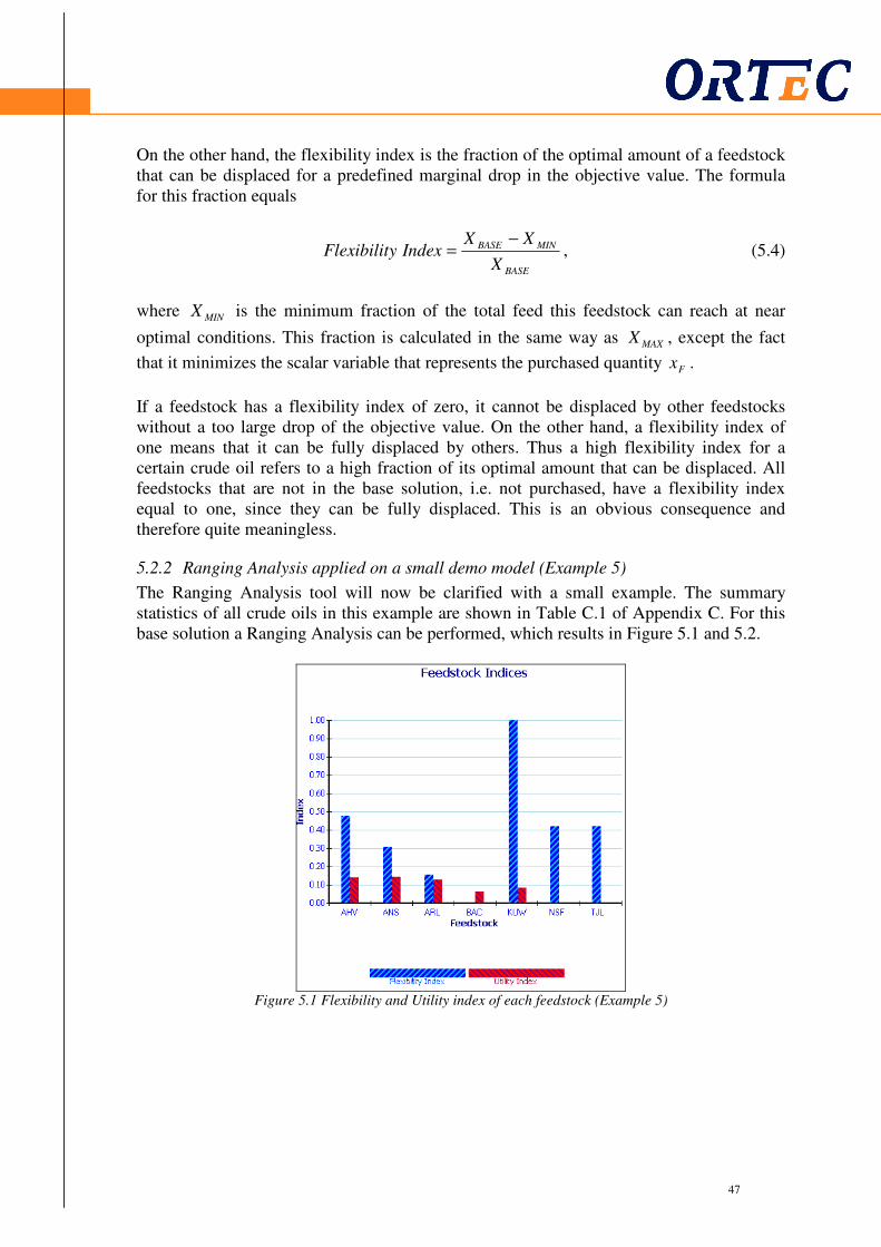
47
47
On the other hand, the flexibility index is the fraction of the optimal amount of a feedstock that can be displaced for a predefined marginal drop in the objective value. The formula for this fraction equals
BASE
MINBASE
X
XXIndexyFlexibilit
−= , (5.4)
where MINX is the minimum fraction of the total feed this feedstock can reach at near
optimal conditions. This fraction is calculated in the same way as MAXX , except the fact
that it minimizes the scalar variable that represents the purchased quantity Fx .
If a feedstock has a flexibility index of zero, it cannot be displaced by other feedstocks without a too large drop of the objective value. On the other hand, a flexibility index of one means that it can be fully displaced by others. Thus a high flexibility index for a certain crude oil refers to a high fraction of its optimal amount that can be displaced. All feedstocks that are not in the base solution, i.e. not purchased, have a flexibility index equal to one, since they can be fully displaced. This is an obvious consequence and therefore quite meaningless.
5.2.2 Ranging Analysis applied on a small demo model (Example 5)
The Ranging Analysis tool will now be clarified with a small example. The summary statistics of all crude oils in this example are shown in Table C.1 of Appendix C. For this base solution a Ranging Analysis can be performed, which results in Figure 5.1 and 5.2.
Figure 5.1 Flexibility and Utility index of each feedstock (Example 5)

48
48
Figure 5.2 The values of MINX , BASEX , and MAXX for each feedstock (Example 5)
The utility and flexibility indices for the different crude oils are shown in Figure 5.1 and
the corresponding MINX , BASEX , and MAXX are shown in Figure 5.2. This last figure gives
information about the range of the quantity of all crude oils. According to Figure 5.1, there are two crude oils that have a utility index of zero in this scenario, namely NSF and TJL. Hence these crude oils cannot displace other crude oils within a predefined marginal drop in the objective value. Thus when (a part of) a certain feedstock cannot be delivered, it cannot be displaced by NSF or TJL. On the other hand, there is no crude oil with a utility index of one, which is as expected. It means that there is no crude oil that can displace the whole remaining total feed and still keeps the objective value at a certain level. If we have a look at the flexibility indices, there is one feedstock with a flexibility index of zero and one with an index equal to one. The crude oil BAC cannot be displaced by other crude oils, without a too large drop of the objective value. On the other hand, the crude oil KUW can be fully displaced by other crude oils. Unfortunately this is quite meaningless, since it is an obvious consequence of the fact that KUW has an activity of zero in the optimal solution. Note that on the other hand, KUW can substitute the original crude slate up to 8% (the utility index value) of the total feed. According to Figure 5.2, the feedstock AHV has the widest range, which means that purchasing this feedstock brings a high degree of flexibility without a user-specified drop in the objective function value. The advantage of Ranging Analysis is that when a certain crude oil can only be purchased less or even not (due to uncertainty in the supply chain), it can determine which crude oil can replace this lack to minimize the decrease in objective function value. Thus it gives a more global view than marginal values on small adjustments in the basic solution. As explained in this section, Ranging Analysis could be an important tool for analysing an optimal solution. Note that instead of feedstocks, the same analysis can be done for end products and capacities. Two other additional features of XNLP will be discussed in the next two sections.

49
49
5.3 Parametric Analysis
5.3.1 Introduction
The Parametric Analysis tool can be used to evaluate cases that parameterize an objective function coefficient of a variable, i.e. to investigate the behaviour of the model as a function of some price changes of a raw material, product, or other variables over a defined range. For instance, it can be investigated what happens with the purchase of a certain crude oil when the price of that crude oil or a different one changes. To clarify this tool, the data of Example 5 will again be used in the next example (Example 6).
5.3.2 Parametric Analysis applied on a small demo model (Example 6)
A Parametric Analysis of the crude oil ‘Arabian Light’, which is also used in Example 5, is shown in Figure 5.3.
Figure 5.3 Parametric Analysis of the crude oil Arabian Light (Example 6)
The price of Arabian Light is shown on the x-axis of Figure 5.3, whereas the purchase (activity) of this crude oil is shown on the y-axis. First notice that the purchase of Arabian Light has only been measured at the integer values of the price, i.e. the lines in Figure 5.3 are meaningless. Let us again start with the values of Table C.1. When the price of Arabian Light equals 17 $/bbl, the quantity of Arabian Light equals 23.8 bbls/day, which is also shown in Figure 5.3. When the price increases by one, the purchase of Arabian Light decreases directly to 20 bbls/day, which is according to Table C.1 its minimum quantity. On the other hand, when the price decreases by one, the purchase jumps directly to its maximum of 40 bbls/day. A similar figure can be developed in which the consequences of the price changes of Arabian Light for the activity of a different crude oil or end product are shown. In Figure 5.4, such a graph is shown for the purchase of the crude oil ‘Alaskan N Slope’.
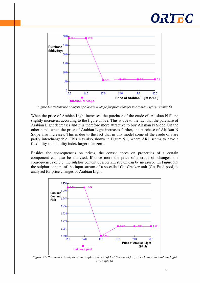
50
50
Figure 5.4 Parametric Analysis of Alaskan N Slope for price changes in Arabian Light (Example 6)
When the price of Arabian Light increases, the purchase of the crude oil Alaskan N Slope slightly increases, according to the figure above. This is due to the fact that the purchase of Arabian Light decreases and it is therefore more attractive to buy Alaskan N Slope. On the other hand, when the price of Arabian Light increases further, the purchase of Alaskan N Slope also increases. This is due to the fact that in this model some of the crude oils are partly interchangeable. This was also shown in Figure 5.1, where ARL seems to have a flexibility and a utility index larger than zero. Besides the consequences on prices, the consequences on properties of a certain component can also be analysed. If once more the price of a crude oil changes, the consequences of e.g. the sulphur content of a certain stream can be measured. In Figure 5.5 the sulphur content of the input stream of a so-called Cat Cracker unit (Cat Feed pool) is analysed for price changes of Arabian Light.
Figure 5.5 Parametric Analysis of the sulphur content of Cat Feed pool for price changes in Arabian Light
(Example 6)
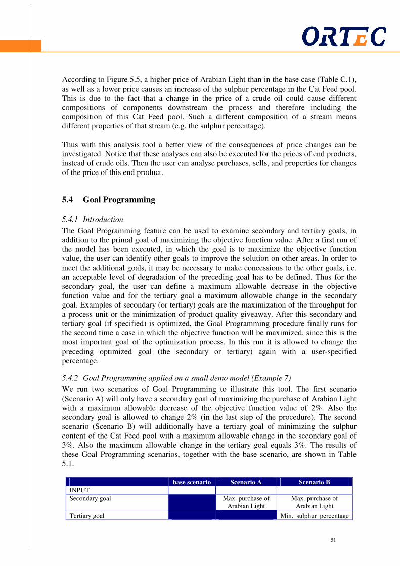
51
51
According to Figure 5.5, a higher price of Arabian Light than in the base case (Table C.1), as well as a lower price causes an increase of the sulphur percentage in the Cat Feed pool. This is due to the fact that a change in the price of a crude oil could cause different compositions of components downstream the process and therefore including the composition of this Cat Feed pool. Such a different composition of a stream means different properties of that stream (e.g. the sulphur percentage). Thus with this analysis tool a better view of the consequences of price changes can be investigated. Notice that these analyses can also be executed for the prices of end products, instead of crude oils. Then the user can analyse purchases, sells, and properties for changes of the price of this end product.
5.4 Goal Programming
5.4.1 Introduction
The Goal Programming feature can be used to examine secondary and tertiary goals, in addition to the primal goal of maximizing the objective function value. After a first run of the model has been executed, in which the goal is to maximize the objective function value, the user can identify other goals to improve the solution on other areas. In order to meet the additional goals, it may be necessary to make concessions to the other goals, i.e. an acceptable level of degradation of the preceding goal has to be defined. Thus for the secondary goal, the user can define a maximum allowable decrease in the objective function value and for the tertiary goal a maximum allowable change in the secondary goal. Examples of secondary (or tertiary) goals are the maximization of the throughput for a process unit or the minimization of product quality giveaway. After this secondary and tertiary goal (if specified) is optimized, the Goal Programming procedure finally runs for the second time a case in which the objective function will be maximized, since this is the most important goal of the optimization process. In this run it is allowed to change the preceding optimized goal (the secondary or tertiary) again with a user-specified percentage.
5.4.2 Goal Programming applied on a small demo model (Example 7)
We run two scenarios of Goal Programming to illustrate this tool. The first scenario (Scenario A) will only have a secondary goal of maximizing the purchase of Arabian Light with a maximum allowable decrease of the objective function value of 2%. Also the secondary goal is allowed to change 2% (in the last step of the procedure). The second scenario (Scenario B) will additionally have a tertiary goal of minimizing the sulphur content of the Cat Feed pool with a maximum allowable change in the secondary goal of 3%. Also the maximum allowable change in the tertiary goal equals 3%. The results of these Goal Programming scenarios, together with the base scenario, are shown in Table 5.1.
base scenario Scenario A Scenario B
INPUT
Secondary goal Max. purchase of Arabian Light
Max. purchase of Arabian Light
Tertiary goal Min. sulphur percentage

52
52
in Cat Feed pool
Max. % change in objective 2% 2%
Max. % change in secondary goal 2% 3%
Max. % change in tertiary goal 3%
OUTPUT
Objective function value 540.02 529.74 529.81
% change in objective function 1.90% 1.89%
Purchase Arabian Light (bbls/day) 23.80 39.21 38.80
% change in secondary goal 1.02%
Sulphur percentage Cat Feed pool 1.891 1.891 1.882
Table 5.1 Goal Programming (Example 7)
According to this figure, the objective function value in Scenario A has been decreased with 1.90% compared to the objective function value in the base scenario. As one can see, this is not equal to the maximum percentage change in the objective value. This is due to the fact that the Goal Programming procedure ends with the main goal (maximizing the objective function), as explained above. To clarify this, the three steps of the Goal Programming procedure in Scenario A are shown in Table 5.2.
Optimize Objective value ($)
Purchase Arabian Light (bbls/day)
Step 1 Objective function 540.02 23.80
Step 2 Purchase Arabian Light 529.22 40.01
Step 3 Objective function 529.74 39.21 Table 5.2 Steps of Goal Programming of Scenario A (Example 7)
Thus in Step 1 of the Goal Programming process the objective function is maximized. Its optimal value equals $540.02, which equals the base scenario of Table 5.1. After that, the purchase of the crude oil Arabian Light is maximized in Step 2, with a maximum decrease in the objective value of 2%. Thus now either the purchase of Arabian Light will reach its upperbound of 50 bbls/day (Table C.1), with a decrease in objective value less than 2%, or the objective value will decrease 2% with the corresponding purchase of Arabian Light. In this case the objective value decreases with 2% (to 529.22). The corresponding amount of Arabian Light that will be purchased equals 40.01 bbls/day (and is indeed less than 50 bbls/day). In Step 3 the objective function value will again be maximized, with a maximum percentage decrease in the amount of purchasing Arabian Light equal to 2%. This eventually results in the solution with an objective function value of $529.74 and a purchase amount of 29.21 bbls Arabian Light per day. Hence the base solution of the model has now slightly been adjusted to obtain a solution in which more goals are fulfilled. Using these three additional features in PIMS, the optimal solution can be analysed and/or finetuned, which gives a better view of the solution and arises the opportunity to obtain a more appropriate solution than in first case. In the following chapters the practical part of the thesis will be elaborated.
53
53
6 Case comparison
6.1 Introduction
The two available solution methods in PIMS (Distributive Recursion and Extended Nonlinear Programming) are extensively outlined in the previous chapters of this thesis. According to Kunt (2003) and Kunt (2004), AspenTech (the developer of PIMS) claims that XNLP performs in general better than DR. In particular they claim less local optima in the XNLP mode, which implies higher objective values on average. They also claim that XNLP needs in general less time to obtain the final solution. These claims will be tested in this chapter, by using models of refineries owned by Shell. The real names of the refineries are not mentioned, but denoted by Refineries A, B, and so on. Note that the linear solver used for both methods is the Xpress solver, which is only used once in the XNLP mode (in the first recursion). In addition, the nonlinear solver in the XNLP mode is the XSLP solver (as explained in Chapter 3).
6.2 Case study
To perform a reliable study and to gain a good overview of the performances of both modes, ten refinery-planning problems will be used for this study. For these ten refineries, a run has been executed in both the Distributive Recursion and the Extended Nonlinear Programming mode. The results of this case study are shown in Appendix D, in which the objective function value, the computation time, and the number of nonzero elements in the matrix are shown. Note that this last statistic is a good indicator for the size of the model. The refineries are ordered from small to large using the number of nonzero elements in the matrix.
Before drawing conclusions about this case study, notice that three out of thirteen models, which gave feasible solutions in the Distributive Recursion mode, did not give feasible solutions or did not even start optimizing in the Extended Nonlinear Programming (XNLP) mode (before optimizing, an error message appears). The reason of this error message could be the fact that all models are build (and therefore the starting points are chosen) to be run in DR and therefore not appropriate to be run in XNLP. However, there is not enough evidence to draw any conclusions about these models. Besides this, AspenTech claims that the starting points (guesses) in the XNLP mode are less important to avoid local optima. This means that obtaining infeasibility in these three models could be in contradiction with the claims of AspenTech. These three models are not used in this case study and not shown in Appendix D. Besides infeasible models, there are also models (Refineries C, D, G, I, and J), which had to be run twice in the XNLP mode to obtain a feasible solution. This happens when the starting point of the run ends up at an infeasible solution. We then use this infeasible solution as starting point in the new run and a feasible solution is obtained. These refinery
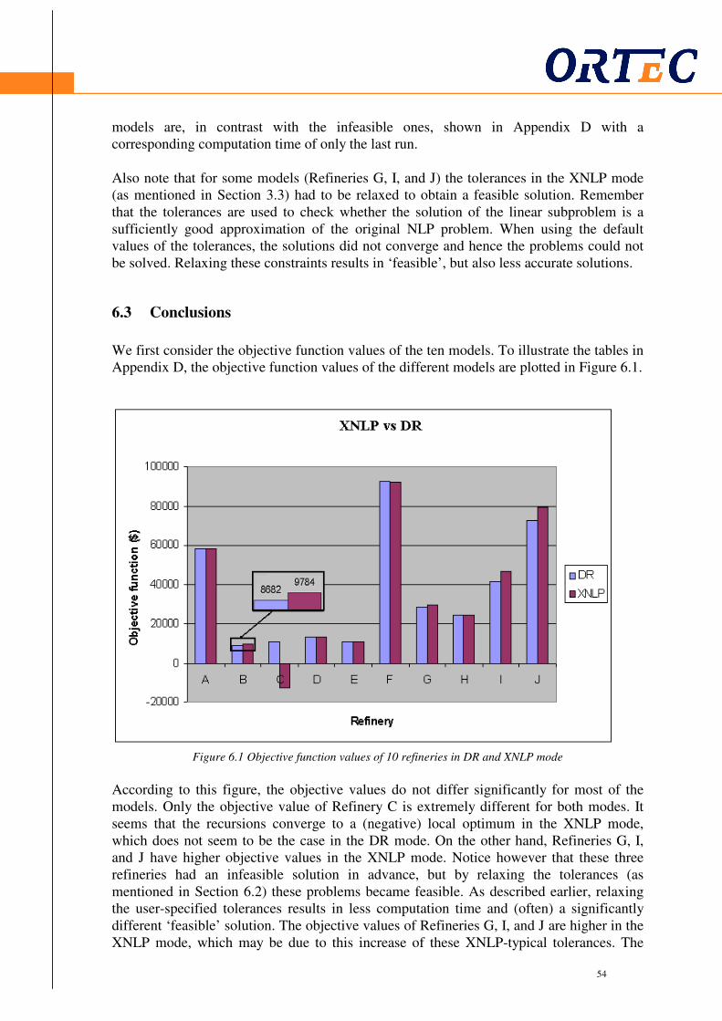
54
54
models are, in contrast with the infeasible ones, shown in Appendix D with a corresponding computation time of only the last run. Also note that for some models (Refineries G, I, and J) the tolerances in the XNLP mode (as mentioned in Section 3.3) had to be relaxed to obtain a feasible solution. Remember that the tolerances are used to check whether the solution of the linear subproblem is a sufficiently good approximation of the original NLP problem. When using the default values of the tolerances, the solutions did not converge and hence the problems could not be solved. Relaxing these constraints results in ‘feasible’, but also less accurate solutions.
6.3 Conclusions
We first consider the objective function values of the ten models. To illustrate the tables in Appendix D, the objective function values of the different models are plotted in Figure 6.1.
Figure 6.1 Objective function values of 10 refineries in DR and XNLP mode
According to this figure, the objective values do not differ significantly for most of the models. Only the objective value of Refinery C is extremely different for both modes. It seems that the recursions converge to a (negative) local optimum in the XNLP mode, which does not seem to be the case in the DR mode. On the other hand, Refineries G, I, and J have higher objective values in the XNLP mode. Notice however that these three refineries had an infeasible solution in advance, but by relaxing the tolerances (as mentioned in Section 6.2) these problems became feasible. As described earlier, relaxing the user-specified tolerances results in less computation time and (often) a significantly different ‘feasible’ solution. The objective values of Refineries G, I, and J are higher in the XNLP mode, which may be due to this increase of these XNLP-typical tolerances. The

55
55
only refinery that gave a significantly (more than 12%) higher objective value in the XNLP mode without the obligation of running twice or relaxing the tolerances is Refinery B. To clarify this difference, the objective function values of Refinery B are enlarged in Figure 6.1. In this case, the objective function value in the DR mode seems to be a local optimum. Note that it is not guaranteed that the objective function value in the XNLP mode is indeed a global optimum, but it is a least a higher local optimum than the one in DR. By considering the objective values, one can conclude that they are in general approximately equal for both modes. This is in contrast with the opinion of AspenTech, who claim that using XNLP results in less local optima and thus higher objective values on average. Considering the computation times of the different models may show us some more differences and could give us a better idea of the functionality of XNLP with respect to DR. A similar figure as Figure 6.1, but now with the computation times on the y-axis is shown below.
XNLP vs DR
0
10
20
30
40
50
60
A B C D E F G H I J
Refinery
co
mp
uta
tio
n t
ime
(m
in)
DR
XNLP
Figure 6.2 Computation time of 10 refineries in DR and XNLP mode
First note that the computation time depends on the capacities of the computer and the guesses at the first iteration. From this figure it can be concluded that when the model size increases, the computation time of XNLP increases on average more than the time of DR, up to a difference in computation times of 350% in Refinery J. For large refineries F – J the computation time is on average twice as large when using XNLP instead of DR. For the smaller models A – E these computation times are approximately equal. After this small case study has been executed, one can conclude that on average Distributive Recursion performs better than Extended Nonlinear Programming at this moment. In this case study there are no refineries, which have a higher objective value plus less computation time in the XNLP mode. Taking into consideration that Distributive Recursion has significantly been improved since its release and Extended Nonlinear
56
56
Programming is a relative new method, the performance of XNLP may increase in the next years. But for now running all models of Shell in XNLP does not seem to increase the total performance of PlanStar/PIMS, by giving more accurate and higher quality solutions. Although DR gives, according to this case study, higher quality solutions, XNLP could still be a useful mode to execute the runs of refinery-planning models, since it generates additional features that can be used to analyse the base solution (as explained in Chapter 5). In Chapter 7 one of these new features (Ranging Analysis) will be implemented in the Marginal Analysis Tool to test whether or not this Ranging Analysis feature could increase the functionality of this tool. Using this test, an answer to the following question will be provided: “How can the additional features be used to improve the functionality of the Marginal Analysis Tool?”.
57
57
7 Ranging Analysis in MAT
7.1 Introduction
Shell uses an Excel template called ‘Marginal Analysis Tool’ (MAT), developed by ORTEC. This tool analyses the solution of the base case, which is optimized with PlanStar/PIMS. This base solution is called the monthly plan of the refinery. As explained in the introduction of this thesis, the user can run cases (prepared with MAT) in which one of the values of a parameter or variable is adapted. Cases can be defined with e.g. a different unit capacity, blend specification, or crude oil import. Thus using MAT, the solution space around the optimum can be explored to gain better understanding of the drivers impacting the margin. In this chapter the emphasis will be on the part of MAT that allows the user to run cases in which the crude oil purchase amounts can be adapted. As explained in the introduction, this part is called Cargo Analysis and in this chapter it is investigated whether the functionality of this analysis can be improved. For the other part of MAT, which is called Marginal Steering (as explained in the introduction), no study will be performed in this chapter to improve its functionality. The input for Cargo Analysis is the monthly plan, updated with the latest information available. The set of crude oils inside this monthly plan is called the base crude diet. It is a feasible crude composition, which is accepted and usually purchased by the refinery. Outside this base crude diet there are a lot of other crude oils available on the market. Using Cargo Analysis it can be evaluated whether one of these crude oils could be a good displacer for one of the crude oils inside the base crude diet. It can also be evaluated whether a crude oil inside the base crude diet could replace a different one, due to delay or unavailability of that crude oil. In Section 7.2 this method will extensively be discussed. According to AspenTech, the new feature Ranging Analysis (explained in Chapter 5), which is only available in the XNLP mode, could give a good overview of the exchangeability of all crude oils. AspenTech claims that Ranging Analysis is very powerful and applicable at two levels, based on Varvarezos (2003). On one hand, the crude oil range can be used as a way to address uncertainty in the availability of crude oils. On the other hand, it can be utilized as a strategic tool for trading and evaluation decisions. The flexibility indices, which are generated during the Ranging Analysis procedure, denote the fraction of its purchase amount that can be displaced by other crude oils, within a predefined decrease in the objective value. As a result, purchasing crude oils with a low flexibility index increases the overall risk. Therefore purchasing crude oils with higher flexibility indices can minimize the risk caused by delay and unavailability of other crude oils. The utility index denotes the fraction of the total feed that can be displaced by the corresponding crude oil, within a predefined decrease in the objective value. Figure 5.1 shows for instance that AHV could replace the highest fraction of the total feed, since it has the highest utility index. Therefore the user can also identify a crude oil with a higher utility index as the “back-up” feed, since that crude oil could replace most others if needed. Utilizing this information (by creating for instance inventory of this particular crude oil) will minimize the risk on operating sub-optimally in the case of an unforeseen

58
58
change in the monthly plan. Hence in this way the indices determined with Ranging Analysis can be useful for the traders. Based on these statements of AspenTech, Shell is excited about this tool and wants to evaluate whether Ranging Analysis could improve the functionality of Cargo Analysis, by implementing the new feature within this old method. In that case Ranging Analysis is used for evaluating all crude oils on the market. If it does not prove to be useful in this case, Ranging Analysis could still be applicable for addressing uncertainty in the availability and as a strategic tool (as described above). This means that investigating the working of this method and comparing it to the current method is anyhow relevant for Shell and ORTEC. Since AspenTech claims that Ranging Analysis gives a good overview of the exchangeability of all crude oils, Shell wants to investigate whether the utility indices of all crude oils outside the base crude diet could give a good representation of which crude oils are appropriate to displace the ones in the base crude diet. Using Ranging Analysis, the functionality of MAT could therefore be improved. However, there are some significant differences between the Ranging Analysis procedure and the current method (Cargo Analysis), such that it probably causes different results in the case study. These differences will be considered in Section 7.3. Since ORTEC predicts that the differences will be of such a degree that Ranging Analysis will not be useful in combination with Cargo Analysis and since case studies are useful to convince Shell, the Ranging Analysis tool has been implemented in MAT (Section 7.4) in order to investigate whether it can improve the functionality of MAT. It is compared to Cargo Analysis, since it already has been proved that this method performs well.
7.2 Current method: Cargo Analysis
At this moment all crude traders at the refineries of Shell use the results of the Cargo Analysis method. On one hand, this analysis is used to investigate whether there are opportunities to increase the refinery margin by purchasing other crude oils that are available on the market, instead of a crude oil in the base crude diet (first goal). On the other hand, it can be investigated which crude oil in the base solution could be appropriate to be purchased more than the optimal value (as inventory), due to uncertainty in the delivery of a crude oil in the base solution (second goal). In the rest of this section the first goal will be explained based on the Cargo Analysis method. The crude oils, which are frequently processed on the refinery and easily available, are usually included in the base crude diet. Most of the purchase amounts of these crude oils are fixed by contracts or already available at the refinery as inventory, when running the Cargo Analysis procedure. Nevertheless there are many other crude oils available on the market, which might add value to the refinery margin. To evaluate these other crude oils on the market, an additional amount of such a crude oil can be forced in a new case. Besides this, the user can specify which amounts of the crude oils purchased in the base crude diet can be replaced in this new case and which ones have to stay fixed. The purchases of the ones that can be replaced are usually easy to cancel. Usually it is always

59
59
the same set of crude oils, which are e.g. transported to the refinery through pipelines (and not by ship), such that they can easily be cancelled. In MAT they are free to move between the minimum and maximum purchase amounts. The other ones keep their actual value of the base solution as fixed value in the new case. In Table 7.1 the monthly plan of an arbitrary refinery is shown. The trader can distinguish the fixed with the free ones by putting crosses at the right side of the table in MAT (see Table 7.1), based on his experience and information.
BASE CASE CRUDE OILS Fixed in BaseCase
Crude oil Input costs MIN MAX ACTUALS
ARAH 169.29 70.0 140.0 70.0 x
ARAL 181.36 0.0 280.0 256.2
BREB 198.16 0.0 160.0 160.0 x
FORC 192.76 0.0 160.0 46.2 x
OMAN 184.20 0.0 140.0 140.0 x
UPZA 187.67 0.0 240.0 0.0 x
Table 7.1 Base solution with corresponding free and fixed crude oils In this table all the crude oils in the base crude diet are shown with corresponding purchase costs (input costs) in $, purchase constraints (MIN and MAX) in kton/month, and actual purchase amount in the base solution (ACTUALS) in kton/month. In Table 7.1 only the crude oil ARAL has not been fixed. This one is called the balancing crude oil. This means that the trader wants to evaluate whether a crude oil is available on the market, which is more appropriate than ARAL. Such a crude oil is more appropriate when it increases the objective value. Thus in the sensitivity cases, which will be prepared by MAT (to be run in PlanStar), the amount of ARAL is allowed to increase or decrease between the minimum and maximum purchase amounts of Table 7.2. Note that in practice this amount will decrease since the capacity to process all the crude oils is in general fully used and the evaluated crude oil is forced in. In Table 7.2 such a case is shown for the crude oil ABCD (which is available on the market but not in the base crude diet). Now a fixed amount of 80 barrels (bbls) will be forced to be in the new case.
Crude oil MIN MAX FIX
ABCD 80
Table 7.2 Additional crude oil that is forced in a new case
Notice that the user can also specify a variable amount, which is added in the new case, by defining a minimum and maximum amount that will be forced (instead of a fixed amount). This occurs less often, since the available sizes are usually fixed and depending on the size of the crude oil tankers/boats. Thus in the new case all the crude oil purchases are fixed to the amount of the base solution, except the one of ARAL (which is free to move) and ABCD (which is forced to be 80 bbls). This new case can be sent to PlanStar/PIMS and a new solution can be calculated. The corresponding objective value gives a good representation of the exchangeability of ARAL by ABCD. When one wants a good overview of the exchangeability of ARAL by all possible crude oils, a large number of cases has to be executed. For all these cases a ‘Crude Indifference Value’ (CIV) in $/bbl is calculated in
60
60
MAT, which is the additional (marginal) value in the objective function value per barrel of the corresponding case with respect to the base solution (Table 7.1). The larger this value, the more attractive the corresponding crude oil. Hence these values are calculated after the cases are run and could therefore give a good rank of the exchangeability of ARAL by all available crude oils outside the base crude diet. This current method used within Shell is an accurate method, but extremely time-consuming since all possible cases have to be run. Using the utility indices of Ranging Analysis in MAT (see expression (5.2)) could reduce this number of cases, by running only cases for those crude oils, which have a relative high utility index. This is since these crude oils can displace the largest fraction of the total feed, with a predefined decrease in objective value. Note that in this case this user-specified decrease in the objective value will usually be 0%. Hence the time necessary to get a good overview of the exchangeability of for instance the crude oil ARAL could be reduced. Therefore it first has to be investigated whether Ranging Analysis could indeed be useful in MAT. Before that, the differences of both methods will first be discussed in the next section.
7.3 Differences between both methods
Although AspenTech claims that Ranging Analysis is a good way to test the exchangeability of balancing crude oils by other crude oils outside the base crude diet, there are some significant differences with the current method of Cargo Analysis. In the current method every case that has been run forces only one crude oil in the base solution and allows only the balancing crude oil to decrease. This base solution contains only the crude oils inside the base crude diet. On top of that, in Ranging Analysis the crude oils that have to be evaluated and that are outside the base crude diet are also free to be purchased in the base solution. This means that this base solution will usually be significantly different than the base solution of Cargo Analysis (with only crude oils from the base crude diet). Since all crude oils are allowed to be purchased in the case of Ranging Analysis, a lot of small drops of different crude oils will be purchased. Since this does not reflect the reality, it can be seen as a shortcoming of the Ranging Analysis procedure. Besides in the base solution, also in the cases to calculate the utility and flexibility indices all purchase amounts can be adapted in Ranging Analysis, which is also not realistic. This is significantly different from allowing only two crude oil amounts to change in the case of Cargo Analysis. The different contents of the base case and other cases are of such a degree that it will be very likely that Ranging Analysis will not improve the functionality of the current Cargo Analysis method. Another difference between both methods is the goal to optimize. In the current Cargo Analysis method the objective function of the model will be maximized, given the base crude diet with one balancing crude oil and one forced crude oil, which is outside the base crude diet. For each of these crude oils a given purchase amount will be forced into the model in separate cases. The only purchase variable in all these cases is the purchase amount of the balancing crude oil. In this method the objective values of these cases may therefore turn out higher than the objective value of the base case. In contrast with Cargo Analysis, Ranging Analysis optimizes the purchase amount, taking into account a

61
61
predefined decrease in the objective function value. This predefined decrease should be specified by the user and can also be 0%. Using this tolerance, the objective value will
decrease to its lowerbound, such that the maximum purchase amount ( MAXX ) can be
calculated. Note that when the trader wants to investigate whether there are opportunities to increase the refinery margin by purchasing other crude oils that are available on the market (the first goal, as explained in Section 7.2), the user-specified decrease in the objective value will usually be 0%. Then only those crude oils, which do not decrease the
objective value, give positive values of MAXX . The purchase amount in Ranging Analysis
is therefore not fixed, but maximized, such that the objective value will not decrease more than the user-specified percentage. This means that both methods have a different goal to optimize. However when only considering this difference, we believe there will still be a positive relation between both methods. If for instance a crude oil performs well in Cargo Analysis, i.e. the corresponding case has a relative high CIV, it is attractive to purchase this crude oil. When it has on the other hand a high utility index with a user-specified drop of 0%, it means that purchasing a relative large amount of this crude oil does not decrease the objective value. We believe these two scenarios are positively correlated. If a crude oil has a negative CIV, it means that it is not attractive to force this crude oil into the base solution, instead of the balancing crude oil. This is also usually positively correlated with a utility index of e.g. zero, which means that the objective function value has to decrease to force this crude oil into the base solution. Considering the differences, it is not straightforward that Ranging Analysis can improve the Cargo Analysis process. However, to advice Shell on this topic, Ranging Analysis will be implemented in MAT, such that both methods can be compared. Though we have our doubts it could not be used for this purpose, it could still be used to address the uncertainty in the availability of crude oils in the base crude diet (the second goal, as explained in Section 7.2).
7.4 Using Ranging Analysis to improve MAT
To reduce the number of cases and therefore the time to obtain a good overview of the exchangeability of the crude oils, the results of the Ranging Analysis procedure can be used in MAT. As explained in Section 5.2, Ranging Analysis could give a good overview of the flexibility of crude oils. Running only those cases for which the forced crude oil has a sufficiently high utility index could reduce the time of the complete process and may therefore improve the functionality of MAT. To clarify this method and to test the differences and similarities, the algorithm in the following subsection has been developed.
7.4.1 Algorithm
Step 1:
• Run PlanStar/PIMS to obtain a base solution of a given model and load it from PlanStar into MAT.
Step 2:
• Divide the crude oils of the base solution in crude oils with fixed and free purchase amounts. The user can do this by putting crosses in the ‘fixed in base case’-column
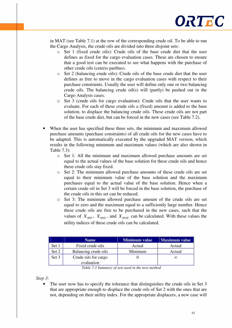
62
62
in MAT (see Table 7.1) at the row of the corresponding crude oil. To be able to run the Cargo Analysis, the crude oils are divided into three disjoint sets:
o Set 1 (fixed crude oils): Crude oils of the base crude diet that the user defines as fixed for the cargo evaluation cases. These are chosen to ensure that a good test can be executed to see what happens with the purchase of other crude oils (ceteris paribus).
o Set 2 (balancing crude oils): Crude oils of the base crude diet that the user defines as free to move in the cargo evaluation cases with respect to their purchase constraints. Usually the user will define only one or two balancing crude oils. The balancing crude oil(s) will (partly) be pushed out in the Cargo Analysis cases.
o Set 3 (crude oils for cargo evaluation): Crude oils that the user wants to evaluate. For each of these crude oils a (fixed) amount is added to the base solution, to displace the balancing crude oils. These crude oils are not part of the base crude diet, but can be forced in the new cases (see Table 7.2).
• When the user has specified these three sets, the minimum and maximum allowed purchase amounts (purchase constraints) of all crude oils for the new cases have to be adapted. This is automatically executed by the upgraded MAT version, which results in the following minimum and maximum values (which are also shown in Table 7.3):
o Set 1: All the minimum and maximum allowed purchase amounts are set equal to the actual values of the base solution for these crude oils and hence these crude oils stay fixed.
o Set 2: The minimum allowed purchase amounts of these crude oils are set equal to their minimum value of the base solution and the maximum purchases equal to the actual value of the base solution. Hence when a certain crude oil in Set 3 will be forced in the base solution, the purchase of the crude oils in this set can be reduced.
o Set 3: The minimum allowed purchase amount of the crude oils are set equal to zero and the maximum equal to a sufficiently large number. Hence these crude oils are free to be purchased in the new cases, such that the
values of MINX , MAXX , and BASEX can be calculated. With these values the
utility indices of these crude oils can be calculated.
Name Minimum value Maximum value
Set 1 Fixed crude oils Actual Actual
Set 2 Balancing crude oils Minimum Actual
Set 3 Crude oils for cargo
evaluation
0 ∞
Table 7.3 Summary of sets used in the new method
Step 3:
• The user now has to specify the tolerance that distinguishes the crude oils in Set 3 that are appropriate enough to displace the crude oils of Set 2 with the ones that are not, depending on their utility index. For the appropriate displacers, a new case will

63
63
be prepared in MAT, similar as the one in Table 7.2. Selection criteria can be of the following forms:
o Absolute criterion: When the utility index of the crude oil is above a certain fraction c a new case will be prepared. Note that using this criterion gives an unknown number of new cases to be run.
o Relative criterion: When the utility index is in the first d %-quantile of all
utility indices, with 1000 ≤≤ d , a case will be prepared. This way, one can control the number of new cases that will be prepared.
Step 4:
• Run the Ranging Analysis procedure for Set 3 with the new minimum and maximum allowed purchase amounts of all crude oils. This results in values of
MINX , MAXX , and BASEX for crude oils in Set 3, as explained in Section 5.2. Thus
MINX is the minimum amount of the crude oil without a predefined drop in the
objective value, and similarly MAXX the maximum. BASEX is the new actual
purchase value of the corresponding crude oil, given the new minimum and maximum allowed purchase amounts of all crude oils.
Step 5:
• Import these calculated values in the upgraded MAT version. The software automatically calculates the utility indices for the crude oils in Set 3, by using expression (5.2). These values give a good representation of the capability of displacing base case crude oils by the ones in Set 3. Hence these values are now used to represent the capability of displacing only the crude oil(s) in Set 2.
Due to the selection criterion described above, the number of cases that are necessary to get a good overview of the exchangeability of crude oils in Set 2 is reduced significantly, such that the complete procedure could be less time-consuming. To clarify this algorithm, an example of a large refinery model (Example 7) will be discussed in the next section.
7.4.2 Example of Ranging Analysis in MAT (Example 7)
A model of a large refinery is used to clarify the method above. This model consists all necessary PlanStar/PIMS data together plus the MAT version with the Ranging Analysis feature. The data contains for instance more than 100 crude oils that can be purchased. Ranging Analysis could give a good overview of the exchangeability of these crude oils, to avoid running more than 90 cases. Step 1:
• The base solution of this example is shown in Table 7.4, which is obtained by running PlanStar/PIMS in the XNLP mode.
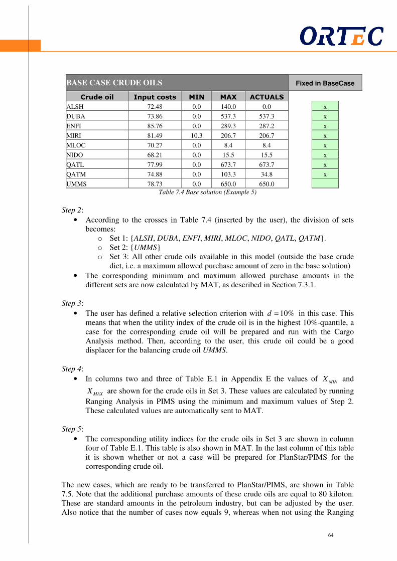
64
64
BASE CASE CRUDE OILS Fixed in BaseCase
Crude oil Input costs MIN MAX ACTUALS
ALSH 72.48 0.0 140.0 0.0 x
DUBA 73.86 0.0 537.3 537.3 x
ENFI 85.76 0.0 289.3 287.2 x
MIRI 81.49 10.3 206.7 206.7 x
MLOC 70.27 0.0 8.4 8.4 x
NIDO 68.21 0.0 15.5 15.5 x
QATL 77.99 0.0 673.7 673.7 x
QATM 74.88 0.0 103.3 34.8 x
UMMS 78.73 0.0 650.0 650.0
Table 7.4 Base solution (Example 5)
Step 2:
• According to the crosses in Table 7.4 (inserted by the user), the division of sets becomes:
o Set 1: {ALSH, DUBA, ENFI, MIRI, MLOC, NIDO, QATL, QATM}. o Set 2: {UMMS} o Set 3: All other crude oils available in this model (outside the base crude
diet, i.e. a maximum allowed purchase amount of zero in the base solution)
• The corresponding minimum and maximum allowed purchase amounts in the different sets are now calculated by MAT, as described in Section 7.3.1.
Step 3:
• The user has defined a relative selection criterion with %10=d in this case. This means that when the utility index of the crude oil is in the highest 10%-quantile, a case for the corresponding crude oil will be prepared and run with the Cargo Analysis method. Then, according to the user, this crude oil could be a good displacer for the balancing crude oil UMMS.
Step 4:
• In columns two and three of Table E.1 in Appendix E the values of MINX and
MAXX are shown for the crude oils in Set 3. These values are calculated by running
Ranging Analysis in PIMS using the minimum and maximum values of Step 2. These calculated values are automatically sent to MAT.
Step 5:
• The corresponding utility indices for the crude oils in Set 3 are shown in column four of Table E.1. This table is also shown in MAT. In the last column of this table it is shown whether or not a case will be prepared for PlanStar/PIMS for the corresponding crude oil.
The new cases, which are ready to be transferred to PlanStar/PIMS, are shown in Table 7.5. Note that the additional purchase amounts of these crude oils are equal to 80 kiloton. These are standard amounts in the petroleum industry, but can be adjusted by the user. Also notice that the number of cases now equals 9, whereas when not using the Ranging

65
65
Analysis procedure, the number of cases is equal to 94. However, the question of whether or not these cases are indeed the most appropriate ones will be answered using a small case comparison in Section 7.5.
Case name Crude oil MIN MAX FIX
T ANGS H801 ANGS 80
T BRNL H801 BRNL 80
T KATA H801 KATA 80
T KEKW H801 KEKW 80
T MADU H801 MADU 80
T SENI H801 SENI 80
T SLLG H801 SLLG 80
T TAPU H801 TAPU 80
T WSEN H801 WSEN 80 Table 7.5 New cases with additional crude oils in Set 3 (Example 5)
This whole procedure has been programmed in Excel, using Microsoft Visual Basic. Hence a new, upgraded version of MAT is available, with an implementation of the Ranging Analysis feature. The added module in MAT is shown in Appendix F, together with the summarized contents and points to improve.
7.5 Comparison of the current and new method
After the complete process has been implemented, it can be tested whether or not the idea of deciding which cases will be run by looking at their utility indices, results in running the most attractive and profitable cases (according to their Crude Indifference Values). In other words, do the current method Cargo Analysis and the method with Ranging Analysis show similar results, such that the functionality of the Marginal Analysis Tool could be improved, given the differences described in Section 7.3?
7.5.1 Comparison of both methods (Example 8)
Two refineries Y and Z are run with both methods to compare the rank of the utility indices with the rank of the CIV’s. Then one can see whether there is a positive correlation between both ranks. The results of these runs are shown in Appendix G. To clarify these tables, the crude oils are sorted by CIV rank and plotted in Figure 7.1 and 7.2.

66
66
0
20
40
60
80
100
120
140
crude oils
ran
k
Rank CIV's
Rank utility indices
CIV's vs Utility indices (Refinery Y)
Fig 7.1 Rank CIV’s versus Rank Utility indices of Refinery Y (Example 8)
Fig 7.2 Rank CIV’s versus Rank Utility indices of Refinery Z (Example 8)
When looking at both figures, it is clear that the blue and pink curves do not show similarities and do not have a positive correlation. This means that the ranks do not show similarities and hence the utility indices are, according to these two models, not appropriate to indicate for which crude oils a case has to be prepared and run. If, for instance, the ten ‘best’ crude oils have to be prepared, the ten crude oils with the lowest rank will be chosen. According to the CIV’s (blue curve), the ten crude oils at the left side of the figure gain the highest marginal profit, when buying 80 kiloton of this crude oil. On the other hand, according to the utility indices (pink curve), the ten lowest points in both
67
67
figures are scattered over the whole x-axis and hence it are mostly other crude oils. So, these crude oils do not give the highest marginal profit, although according to the new method they seem to do. In other words, the difference between the rank of cases that are chosen by utility indices and that are chosen by CIV’s are extremely different, such that the utility indices cannot be used for this purpose. The main reason of this dissimilarity is the first difference of Section 7.3. Thus the base solution of Ranging Analysis will usually be significantly different than the base solution of Cargo Analysis (with only crude oils from the base crude diet) and therefore the ranks for both methods do also not correlate.
7.5.2 Conclusions and motivation
One can conclude that, according to these two models, Ranging Analysis is indeed not useful to increase the functionality of the Marginal Analysis Tool, by choosing the most appropriate cases based on the highest utility indices. It means that the differences between the current method and the one with Ranging Analysis, which are explained in Section 7.3, are (as expected) of such a degree that different results are obtained. The results of Cargo Analysis are more accurate, since they are calculated afterwards. It is therefore not attractive to replace the current version of Cargo Analysis, since the results of the implemented version with Ranging Analysis are not good enough. Also notice that the time of the complete process is at this moment not significantly less than in the old method. Even though the number of cases to be run has been reduced, the time required for running Ranging Analysis to obtain the utility indices is large, such that the completion time is approximately equal. However, the case study is still very useful since it assists explaining the differences to Shell and the conclusion that Ranging Analysis cannot improve Cargo Analysis in this way. According to the case study, Ranging Analysis is not suitable for the first goal of Cargo Analysis to be implemented within the current Cargo Analysis method. This is mainly due to the first difference explained in Section 7.3. Both calculation methods are namely based on a different base case: Ranging Analysis is based on all crude oils on the market, whereas Cargo Analysis is only based on the base crude diet. However, it could still be used for other purposes. The utility and flexibility indices of the base crude oils are still relevant for the trader at two levels. On one hand, it can still be used as a way to address uncertainty in the feedstock availability (second goal of Cargo Analysis), since for this purpose only the crude oils inside the base crude diet are analysed and then Ranging Analysis works well (see Section 5.2). On the other hand, Ranging Analysis can be utilized as a strategic tool for trading. The user could e.g. identify an additional amount of a base crude oil with a high utility index as inventory and minimize crude oils with low flexibility indices. Also for this analysis the base solution only contains crude oils of the base crude diet. Utilizing this information will minimize the risk of operating sub-optimally in the case of an unforeseen change in the monthly plan. This means that the implementation of Ranging Analysis in MAT could still be useful for other purposes.
7.5.3 Recommendations
In this chapter the Ranging Analysis procedure has been implemented in the Marginal Analysis Tool to improve its functionality. As explained in Section 7.1, Ranging Analysis has only been implemented in the Cargo Analysis part of MAT. For this part it has been shown that, by looking at the case study of Section 7.5, the utility indices do not help
68
68
filtering the most attractive cases. At the end of this chapter the following recommendations for further research of Ranging Analysis and MAT may be considered:
• The first difference from Section 7.3 is caused by the structure of the Ranging Analysis procedure. As explained earlier, it is not realistic when all crude oils can be purchased in the base solution. If AspenTech adjusts the Ranging Analysis procedure, this problem can be solved. When this difference disappears, Ranging Analysis could be more useful to improve the first goal of Cargo Analysis and therefore a new study should be executed. Since the second difference of Section 7.3 is less relevant, this new study will probably gain better results.
• When using Ranging Analysis for the first goal of Cargo Analysis (see Section 7.2), all purchase amounts are free to move to obtain a reliable value. This often results in purchasing a lot of small drops of different crude oils. In reality this is often not desirable and possible. Therefore dummy variables could be added to the process to ensure that the purchase amounts of the crude oils are at least one cargo (e.g. 80 kiloton), such that no small drops can be purchased. This is more realistic and the method shows more similarities with Cargo Analysis. When the user wants for instance a minimum purchase amount of b kiloton (if it is purchased) and an allowable drop in the objective value of ε (which will usually be zero in this case),
the purchase constraints have to be defined as:
iii ICXIb ⋅≤≤⋅ , (7.1)
where C is a sufficiently large number, iX the purchase amount for crude oil i, and
else,
function objective base )-(1 function objective if
0
1 ⋅≥
=ε
iI
for crude oil i. Besides this, the following constraint also has to be added to ensure that not more than one crude oil is purchased:
{ }
1,...,1
≤∑∈ Mi
iI , (7.2)
where M is the number of crude oils available on the market. Now crude oil i will only be purchased when an amount of at least b kiloton does not result in a decrease of the objective value (assuming 0=ε ). Thus if a certain crude oil would
have an optimal purchase amount which is less than b, it will not be purchased in the adjusted version of Ranging Analysis, due to the additional constraint (7.1). On the other hand, the small amount will be purchased in the current version of Ranging Analysis. Hence adding constraint (7.1) would make it more realistic and more in line with Cargo Analysis. Since, according to (7.2), there could also not be purchased more than one crude oil each case, the procedure approaches the Cargo Analysis method. Hence using this idea could improve the functionality of Ranging Analysis in combination with Cargo Analysis, for evaluating all crude oils on the market.
69
69
• Also for the Marginal Steering part of MAT, Ranging Analysis could be implemented. With Ranging Analysis one also has the opportunity to analyse product sales, capacities, and other constraints. A small investigation has been executed to evaluate the performance of Ranging Analysis in Marginal Steering. When only running the Ranging Analysis procedure for capacities and products in PIMS (without implementing the utility indices into MAT), the characteristics seem to be the same as running Ranging Analysis for crude oils. This means that the same differences as explained in Section 7.3 may appear in the Marginal Steering part of MAT. However, since Marginal Steering works significantly different than Cargo Analysis and since the whole procedure has not been implemented in MAT, a case study as described in this chapter could be executed. To perform such a case study, a similar module can be added in MAT. This has not been done in this thesis, but could be a study to perform in the future by ORTEC and/or Shell.
70
70
8 Conclusions and recommendations The objective of this thesis was to investigate the mathematics and the functionality of the new nonlinear solution method XNLP available in PIMS. To achieve this goal, four research questions had to be answered. In Section 8.1 the conclusions are shown, which can be drawn concerning these questions and main goal. Furthermore, in Section 8.2 the corresponding recommendations according to this thesis and for further research are discussed.
8.1 Conclusions
The first research question of this thesis is: “How do the two solution methods Distributive Recursion and Extended Nonlinear Programming work on mathematical level?”. As explained in Chapter 1, the current mode Distributive Recursion is based on the Successive Linear Programming (SLP) method, in which the nonlinear problem is represented in PIMS as a linear problem, by presuming some of the variables as known. Since PIMS transforms the NLP problem into linear subproblems, only linear solvers are used to solve the problems. To compensate the error in the guesses of some of the variables (to transform the NLP into an LP problem), an error variable is introduced, which is also optimized in every LP subproblem. Using user-specified tolerances it is decided whether the solution of the LP problem is a sufficiently good approximation of the optimal solution of the NLP problem or a new guess has to be made to start a new iteration with a new LP problem. On the other hand, the new mode Extended Nonlinear Programming does not send an LP to a linear solver. Instead, an NLP is sent to a nonlinear solver. In PIMS there are two nonlinear solvers available, XSLP and CONOPT, which can be used in this mode. The XSLP solver is also based on a Successive Linear Programming method, but significantly differs from Distributive Recursion, since the linearization happens inside the solver and uses first order Taylor expansions. The other nonlinear solver CONOPT is based on a Generalized Reduced Gradient method. The idea of this method is that under certain assumptions all variables can be expressed in terms of an independent subset of the variables, such that the number of variables is reduced. The second research question is: “How appropriate are the nonlinear solvers, which are available in PIMS, for solving refinery-planning problems, compared to other major nonlinear solvers?”. To provide a reliable answer, two other prominent nonlinear solvers (SNOPT and MINOS) have been discussed in Chapter 4. After investigating these other two solvers and comparing them to the two available in PIMS, it can be concluded that XSLP and CONOPT are in general appropriate solvers for refinery-planning problems. The third question of this thesis was: “To what extent does XNLP provide more accurate and higher quality solutions in the refinery planning area?”. Therefore a case study has been executed, which shows us that for ten refinery models of Shell Extended Nonlinear Programming does not perform on average better than Distributive Recursion. Though

71
71
AspenTech claims less local optima when using XNLP, the objective function values are usually not higher than when using DR. Besides that, the computation times are, especially for the larger models, significantly larger in the XNLP mode. Although the performance of XNLP may not be better than DR at this moment, there are some additional features available in the XNLP mode, which may be very useful for the user. The first feature Ranging Analysis gives the user the opportunity to analyse the range under optimality conditions, for each feedstock, product, or capacity. A second additional feature, called Parametric Analysis, can be used to evaluate cases in which variables are analysed when prices of components or products have changed. The last additional feature is Goal Programming. Using this feature, the model can be optimized with a secondary (and tertiary) goal in addition to the primal goal of maximizing the profit. The additional feature Ranging Analysis can be used as a way to address uncertainty in the feedstock availability, which is one of the goals of Cargo Analysis in the Marginal Analysis Tool. It can also be utilized as a strategic tool for trading, such that the risk of operating sub-optimally in the case of an unforeseen change in the monthly plan has been minimized. In this way one of the additional features could therefore be used to improve the Marginal Analysis Tool (fourth research question). It is also shown in this thesis that Ranging Analysis could not improve the functionality of Cargo Analysis, when the goal is to evaluate whether there are opportunities to increase the refinery margin. This is done by purchasing other crude oils in the base solution, instead of a crude oil in the base crude diet. The main reason that that Ranging Analysis does not improve the functionality of Cargo Analysis is that the base solution of Cargo Analysis is only based on the crude oils inside the base solution. Besides that, the base solution in Ranging Analysis could also contain the other crude oils that are available on the market. This means that this base solution will usually be significantly different than the base solution of Cargo Analysis (with only crude oils from the base crude diet), which results in different outcomes. This result has been obtained by investigating both methods and implementing the Ranging Analysis procedure in MAT, such that it could be compared with the current Cargo Analysis method. Hence by answering these four research questions, the mathematics and the functionality of the new nonlinear solution method XNLP available in PIMS are investigated and a good overview of the solution methods in PIMS has been gained.
8.2 Recommendations & further research
8.2.1 Recommendations
According to the conclusions above, the recommendation is to keep using Distributive Recursion to solve the refinery-planning problems at the refineries of Shell. At this moment Extended Nonlinear Programming does not outperform Distributive Recursion, by looking at the objective function values and computation times of the case study in Chapter 6.

72
72
Using Chapter 7 it is also shown that Ranging Analysis does not improve the Cargo Analysis procedure in MAT, when the goal is to evaluate opportunities to increase the refinery margin. Hence running all possible cases is at this moment still the best manner. However, the trader at the refinery could still use Ranging Analysis in MAT, as explained in the previous section.
8.2.2 Further Research
In this thesis Distributive Recursion has been compared to Extended Nonlinear Programming. In practice, only the XSLP solver of XNLP has been used, due to the absence of a CONOPT license. Using the CONOPT solver may give other results than using the XSLP solver and therefore evaluating this solver is a good subject for further research. Besides Cargo Analysis, the other part of MAT, which is called Marginal Steering, could also be evaluated in combination with Ranging Analysis. The principle of Marginal Steering is slightly different than Cargo Analysis and it may therefore give other results than the research of Cargo Analysis in Chapter 7. In this thesis only the Ranging Analysis feature has been implemented in the Marginal Analysis Tool. Further research about the possibility to implement the other additional features (Parametric Analysis and Goal Programming) in MAT may give interesting results and might increase the functionality of MAT. It may also be considered to discuss the bottlenecks and pitfalls, which have been found during the whole process, with AspenTech. AspenTech could also explain why they believe optimizing with XNLP results in less local optima. Discussing the first two recommendations of Subsection 7.5.3 could assist improving Ranging Analysis, by making it more compatible for Shell. Then it could also be discussed why they think that the additional output, generated with XNLP, could be useful for Shell. Note that XNLP therefore first has to perform better than DR before considering using the additional output.

73
73
References
Abadie, J. and Carpentier, J. (1969). Generalization of the Wolfe Reduced Gradient method to the case of nonlinear constraints. Revenue Optimisation, 37-47. Academic Press. Aspen Technology (1998). Process Industry Modeling System Training Manual. Houston, United States of America. Bazaraa, S., Sherali, D., and Shetty, C.M. (1993). Nonlinear Programming, Theory and Algorithms, pp. 432-438. Canada. Cai, X., McKinney, D.C., Lasdon, L.S., and Watkins, D. (2001). Solving large nonconvex water resources management models using generalized Benders decomposition. Operations Research 49(2) 235-245. Griffith, R.E. and Stewart, R.A. (1961). “A Nonlinear Programming Technique for the Optimization of Continuous Processing Systems,” Management Science, 7, pp.379-392. http(1). http://us.ortec.com/solutions/consul.aspx. December, 2007. http(2). http://www.aimms.com/aimms/product/solvers. December, 2007. http(3). http://www.conopt.com/Algorithm.htm. December, 2007. http(4). http://www-fp.mcs.anl.gov/otc/Guide/SoftwareGuide/Blurbs/sqopt_snopt.html. November, 2007. http(5). http://www.gams.com/docs/minosvsconopt.htm. October, 2007. http(6). http://www.ortec.com. May, 2007. http(7). http://www.sbsi-sol-optimize.com/asp/sol_product_snopt.htm. October, 2007. http(8). http://www.tomopt.com/tomlab/products/snopt/solves/SNOPT.php. October, 2007. de Klerk, E., Roos, C., and Terlaky, T. (2005). Course Notes: Optimization (WI4 207). Delft University of Technology, Delft, The Netherlands. Kunt, T. (2003). XNLP: What, Why, and How. AspenTech, presentation at PIMS User Conference. Kunt, T. (2004). Why use XNLP – a case study. AspenTech, white paper from http://support.aspentech.com. Lee, H., Chen, S., and Kang, H. (2004). A Study of Generalized Reduced Gradient Method with Different Search Directions, pp. 25-38. Taichung, Taiwan.
74
74
Moré, J.J. and Wright, S.J. (1993). Optimization Software Guide. Society for Industrial and Applied Mathematics. Philadelphia, United States of America. Nocedal, J and Wright, S.J. (1999). Numerical Optimization. Springer Series in Operations Research . New York, United States of America. Pike, R.W. (2001). Multi variable optimization procedures In Pike, R.W. (2001). Optimization for Engineering Systems. Louisiana State University, United States of America. Poku, B., Biegler, T., Kelly, D., Coxhead, R., and Gopal, V. (2003). Nonlinear programming algorithms for large nonlinear gasoline blending problems. Proceedings of FOCAPO 2003, pp. 605 – 608. Varvarezos, D. (2003). Optimal Feedstock Range Analysis in Refining Production Planning. Paris, France. Wolfe, P. (1963), Methods of Nonlinear Programming. In Recent Advance in Mathematical Programming, Graves, R.L., and Wolfe, P (eds), pp. 67-86. New York: McGaw-Hill, United States of America.
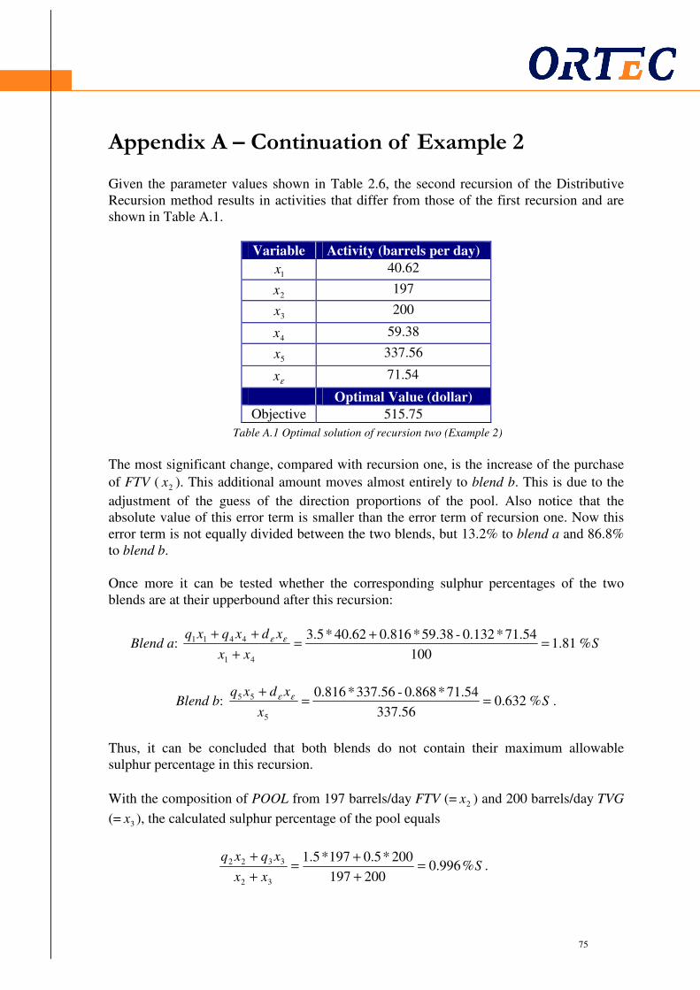
75
75
Appendix A – Continuation of Example 2 Given the parameter values shown in Table 2.6, the second recursion of the Distributive Recursion method results in activities that differ from those of the first recursion and are shown in Table A.1.
Variable Activity (barrels per day)
1x 40.62
2x 197
3x 200
4x 59.38
5x 337.56
εx 54.71
Optimal Value (dollar)
Objective 515.75
Table A.1 Optimal solution of recursion two (Example 2)
The most significant change, compared with recursion one, is the increase of the purchase
of FTV ( 2x ). This additional amount moves almost entirely to blend b. This is due to the
adjustment of the guess of the direction proportions of the pool. Also notice that the absolute value of this error term is smaller than the error term of recursion one. Now this error term is not equally divided between the two blends, but 13.2% to blend a and 86.8% to blend b. Once more it can be tested whether the corresponding sulphur percentages of the two blends are at their upperbound after this recursion:
Blend a: Sxx
xdxqxq%81.1
100
71.54*0.132-59.38*816.040.62*3.5
41
4411 =+
=+
++ εε
Blend b: Sx
xdxq%632.0
337.56
71.54*0.868-337.56*0.816
5
55 ==+ εε .
Thus, it can be concluded that both blends do not contain their maximum allowable sulphur percentage in this recursion.
With the composition of POOL from 197 barrels/day FTV (= 2x ) and 200 barrels/day TVG
(= 3x ), the calculated sulphur percentage of the pool equals
Sxx
xqxq%996.0
200197
200*5.0197*5.1
32
3322 =+
+=
+
+.

76
76
Now we see that the sulphur percentage is almost equal to the maximum allowable percentage, since the sulphur percentage of blend b can be at most 1 %S. To check whether these outcomes are appropriate for the original model, ATol and RTol have to be calculated once more:
.001.0221.0816.0
816.0996.0
001.0180.0816.0996.0
>=−
=
>=−=
RTol
ATol
Thus one can conclude that a new recursion has to be done, to obtain a sufficiently good
solution. Therefore, the new εd has to be calculated again:
150.0200197
38.59=
+=εd .
Hence, the presumed parameter values for recursion three become:
Parameter Value
bq 0.996
εd 0.150
Table A.2 Presumed parameter values for recursion three (Example 2)
These recursions are automatically repeated until the tolerances are small enough and an appropriate, optimal solution has been obtained. For this example, it takes four recursions to obtain a solution with tolerances smaller than 0.001. It results in the following activities and objective value shown in Table A.3.
Variable Activity (barrels per day)
1x 40
2x 200
3x 200
4x 60
5x 340
Optimal Value (dollar)
Objective 520
Table A.3 Optimal solution determined with distributive recursion (Example 2)
As shown in Table A.3, the components FTV and TVG are purchased maximally, in contrast to the amount of SRS. Also the optimal distribution term can now be calculated:
150.0200200
60=
+=εd .
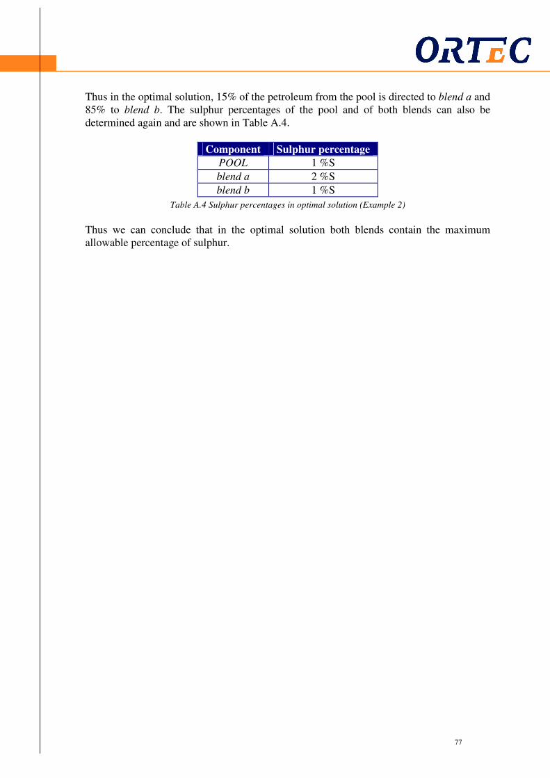
77
77
Thus in the optimal solution, 15% of the petroleum from the pool is directed to blend a and 85% to blend b. The sulphur percentages of the pool and of both blends can also be determined again and are shown in Table A.4.
Component Sulphur percentage
POOL 1 %S
blend a 2 %S
blend b 1 %S
Table A.4 Sulphur percentages in optimal solution (Example 2)
Thus we can conclude that in the optimal solution both blends contain the maximum allowable percentage of sulphur.

78
78
Appendix B – Continuation of Example 4 Iteration 2 Step 1: The Jacobian A and the corresponding vector b can now be calculated, using the new values of x at t=1.
( ) ( ) ( )500.15888.442)( 1|21|1
2
1
1
11 ==
∂
∂
∂
∂=== === ttt xx
x
h
x
hBNxJHA ,
and
( ) 000.72875.3
444.2500.15888.41 =
== =tAxb .
Step 2: Now the basic variable 1|2 =tx can once more be written as a function of the non-
basic variable 1|1 =tx :
1
1
1
11
2 10154.3645.4 xNxBbBx −−− ⋅−=−= .
Step 3: Using this, model (3.7) can be written as a model with only the variable 1|1 =tx . For
simplicity, the term t=1 has been omitted.
(B.1)
Step 4: Now the search directions at t=1 of the basic and the non-basic part have to be determined:
,000.2720.13796.4)(
1|1
1
1|1
1|11| =+−=−== =
=
== t
tN
ttN xx
xfss
δ
δ
and
Step 5: Again the expressions for the new variables can be determined by using the search directions determined above.
(B.2a)
.0
010154.3645.4..
304.86720.13398.2min
1
1
1
1
2
1
≥
≥⋅−
+−−
x
xts
xx
.10308.6000.2889.4500.15
1 1
1|
1
1|21|
−=
−== ⋅−=⋅−=−== tNttB NsBss
0000.2444.21|1|12|1 ≥+=+= === λλ tNtt sxx
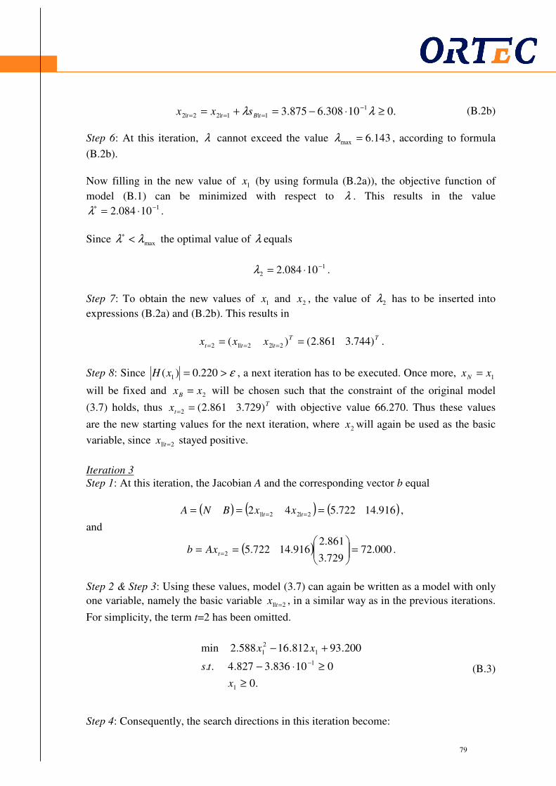
79
79
(B.2b)
Step 6: At this iteration, λ cannot exceed the value 143.6max =λ , according to formula
(B.2b).
Now filling in the new value of 1x (by using formula (B.2a)), the objective function of
model (B.1) can be minimized with respect to λ . This results in the value 110084.2 −∗ ⋅=λ .
Since maxλλ <∗ the optimal value of λ equals
1
2 10084.2 −⋅=λ .
Step 7: To obtain the new values of 1x and 2x , the value of 2λ has to be inserted into
expressions (B.2a) and (B.2b). This results in
TT
ttt xxx )744.3861.2()( 2|22|12 == === .
Step 8: Since ε>= 220.0)( 1xH , a next iteration has to be executed. Once more, 1xxN =
will be fixed and 2xxB = will be chosen such that the constraint of the original model
(3.7) holds, thus T
tx )729.3861.2(2 == with objective value 66.270. Thus these values
are the new starting values for the next iteration, where 2x will again be used as the basic
variable, since 2|1 =tx stayed positive.
Iteration 3 Step 1: At this iteration, the Jacobian A and the corresponding vector b equal
( ) ( ) ( )916.14722.542 2|22|1 === == tt xxBNA ,
and
( ) 000.72729.3
861.2916.14722.52 =
== =tAxb .
Step 2 & Step 3: Using these values, model (3.7) can again be written as a model with only
one variable, namely the basic variable 2|1 =tx , in a similar way as in the previous iterations.
For simplicity, the term t=2 has been omitted.
(B.3)
Step 4: Consequently, the search directions in this iteration become:
.010308.6875.3 1
1|1|22|2 ≥⋅−=+= −=== λλ tBtt sxx
.0
010836.3827.4..
200.93812.16588.2min
1
1
1
2
1
≥
≥⋅−
+−−
x
ts
xx
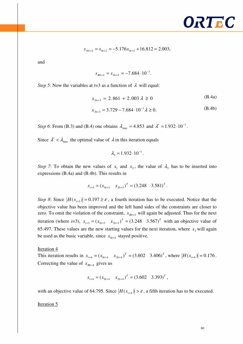
80
80
,003.2812.16176.5 2|12|12| =+−== === tttN xss
and
Step 5: Now the variables at t=3 as a function of λ will equal:
(B.4a)
(B.4b)
Step 6: From (B.3) and (B.4) one obtains 853.4max =λ and 110932.1 −∗ ⋅=λ .
Since maxλλ <∗ the optimal value of λ in this iteration equals
1
3 10932.1 −⋅=λ .
Step 7: To obtain the new values of 1x and 2x , the value of 3λ has to be inserted into
expressions (B.4a) and (B.4b). This results in
TT
ttt xxx )581.3248.3()( 3|23|13 == === .
Step 8: Since ε≥== 197.0)( 3txH , a fourth iteration has to be executed. Notice that the
objective value has been improved and the left hand sides of the constraints are closer to
zero. To omit the violation of the constraint, 3| =tBx will again be adjusted. Thus for the next
iteration (where i=3), TT
ttt xxx )567.3248.3()( 3|23|13 == === with an objective value of
65.497. These values are the new starting values for the next iteration, where 2x will again
be used as the basic variable, since 2|1 =tx stayed positive.
Iteration 4
This iteration results in TT
ttt xxx )406.3602.3()( 4|24|14 == === , where 176.0)( 4 ==txH .
Correcting the value of 4| =tBx gives us
TT
ttt xxx )393.3602.3()( 4|24|14 == === ,
with an objective value of 64.795. Since ε>= )( 4txH , a fifth iteration has to be executed.
Iteration 5
.10684.7 1
2|22|
−== ⋅−== ttB ss
0003.2861.23|1 ≥+== λtx
.010684.7729.3 1
3|2 ≥⋅−= −= λtx
81
81
In this iteration, T
tx )223.3922.3(5 == and 158.0)( 4 ==txH , which is smaller than ε .
That means that the algorithm stops after this iteration. The calculated value for
5|25| == = ttB xx has to be adjusted, to obtain the right solution. This eventually gives us the
optimal solution T
tx )211.3922.3(5 == with an objective value 64.162.

82
82
Appendix C – Summary statistics of Example 5
Obj value ($) 540.02
Feedstocks Amount
(bbls/day) Marginal
value MIN
(bbls/day) MAX
(bbls/day) Price
($/day)
Arabian Heavy 25.196 0.000 0.00 50.00 15.00
Alaskan N Slope 5.722 0.000 0.00 33.00 17.50
Arabian Light 23.804 0.000 20.00 50.00 17.00
Bachequero 1.000 -0.754 1.00 8.00 14.75
Kuwait Export 0.000 0.000 0.00 20.00 16.25
North Sea Forties 20.000 0.594 0.00 20.00 18.30
Tiajuana Light 10.000 0.000 0.00 25.00 17.70 Table C.1 Summary statistics (Example 5)
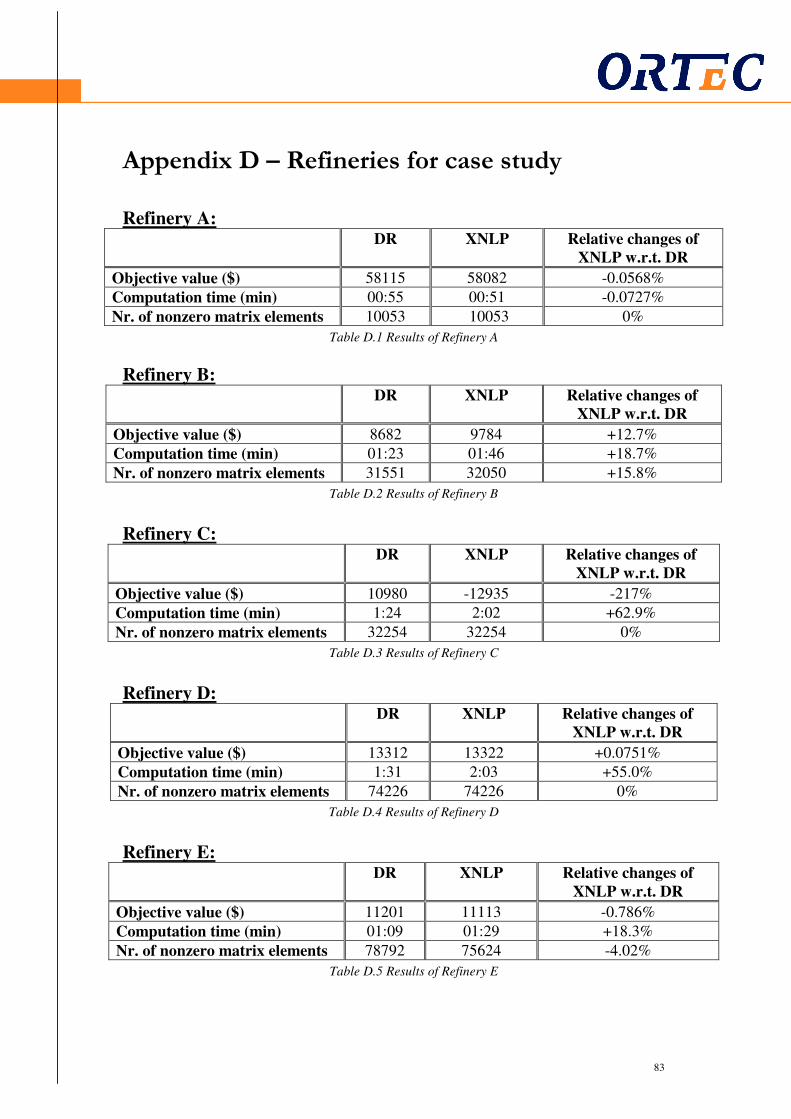
83
83
Appendix D – Refineries for case study
Refinery A:
DR XNLP Relative changes of XNLP w.r.t. DR
Objective value ($) 58115 58082 -0.0568%
Computation time (min) 00:55 00:51 -0.0727%
Nr. of nonzero matrix elements 10053 10053 0%
Table D.1 Results of Refinery A
Refinery B: DR XNLP Relative changes of
XNLP w.r.t. DR
Objective value ($) 8682 9784 +12.7%
Computation time (min) 01:23 01:46 +18.7%
Nr. of nonzero matrix elements 31551 32050 +15.8%
Table D.2 Results of Refinery B
Refinery C:
DR XNLP Relative changes of XNLP w.r.t. DR
Objective value ($) 10980 -12935 -217%
Computation time (min) 1:24 2:02 +62.9%
Nr. of nonzero matrix elements 32254 32254 0%
Table D.3 Results of Refinery C
Refinery D:
DR XNLP Relative changes of XNLP w.r.t. DR
Objective value ($) 13312 13322 +0.0751%
Computation time (min) 1:31 2:03 +55.0%
Nr. of nonzero matrix elements 74226 74226 0%
Table D.4 Results of Refinery D
Refinery E:
DR XNLP Relative changes of XNLP w.r.t. DR
Objective value ($) 11201 11113 -0.786%
Computation time (min) 01:09 01:29 +18.3%
Nr. of nonzero matrix elements 78792 75624 -4.02%
Table D.5 Results of Refinery E

84
84
Refinery F: DR XNLP Relative changes of
XNLP w.r.t. DR
Objective value ($) 92584 92011 -0.619%
Computation time (min) 06:54 19:02 +191%
Nr. of nonzero matrix elements 81598 82438 +1.03%
Table D.6 Results of Refinery F
Refinery G:
DR XNLP Relative changes of XNLP w.r.t. DR
Objective value ($) 28749 29557 +2.81%
Computation time (min) 05:28 09:52 +80.3%
Nr. of nonzero matrix elements 147979 137239 -7.26%
Table D.7 Results of Refinery G
Refinery H:
DR XNLP Relative changes of XNLP w.r.t. DR
Objective value ($) 24403 24422 +0.0779%
Computation time (min) 5:31 18:53 +249%
Nr. of nonzero matrix elements 161638 139361 -13.8%
Table D.8 Results of Refinery H
Refinery I:
DR XNLP Relative changes of XNLP w.r.t. DR
Objective value ($) 41599 46541 +11.9%
Computation time (min) 04:15 13:39 +223%
Nr. of nonzero matrix elements 181639 163403 -10.0%
Table D.9 Results of Refinery I
Refinery J:
DR XNLP Relative changes of XNLP w.r.t. DR
Objective value ($) 72759 79165 +8.80%
Computation time (min) 11:42 51:34 +350%
Nr. of nonzero matrix elements 365926 349426 -4.51%
Table D.10 Results of Refinery J

85
85
Appendix E – Outcomes of Example 7
Crude oil Xbase Xmax Utility index
Appropriate
to run case
AMNA 0.00 8.13 0.18 NO
ANGS 0.00 16.71 0.37 YES
ARAH 0.00 0.00 0.00 NO
ARAL 0.00 0.00 0.00 NO
ARAM 0.00 0.00 0.00 NO
ARJU 0.00 13.37 0.30 NO
ARSL 0.00 7.34 0.16 NO
ARUN 0.00 10.50 0.24 NO
ARXL 0.00 8.63 0.19 NO
BAHO 0.00 8.52 0.19 NO
BASL 0.00 0.00 0.00 NO
BENC 0.00 8.59 0.19 NO
BINC 0.00 0.00 0.00 NO
BONL 0.00 8.04 0.18 NO
BREB 0.00 7.54 0.17 NO
BRNL 0.00 13.90 0.31 YES
BUKH 13.68 16.22 0.08 NO
BUKN 0.00 0.00 0.00 NO
CABD 0.00 7.12 0.16 NO
CAKE 16.11 19.47 0.12 NO
CANU 0.00 2.75 0.06 NO
CHEX 0.00 4.20 0.09 NO
COSB 0.00 9.20 0.21 NO
CYRU 0.00 0.00 0.00 NO
DOBA 0.00 4.03 0.09 NO
DURI 0.00 2.24 0.05 NO
ERHA 0.00 7.01 0.16 NO
ESPA 0.00 2.46 0.06 NO
FORC 0.00 5.77 0.13 NO
GIRA 0.00 6.75 0.15 NO
GULS 0.00 0.00 0.00 NO
HAND 0.00 10.30 0.23 NO
HOUT 0.00 0.00 0.00 NO
IBMS 0.00 0.00 0.00 NO
IRNH 0.00 0.00 0.00 NO
IRNL 0.00 1.76 0.04 NO
JATI 0.00 2.69 0.06 NO
KAJI 0.00 9.48 0.21 NO
KATA 0.00 16.75 0.38 YES
KEKW 0.00 14.15 0.32 YES
KHAF 0.00 0.00 0.00 NO
KHUF 0.00 12.24 0.27 NO
KIDU 0.00 9.17 0.21 NO
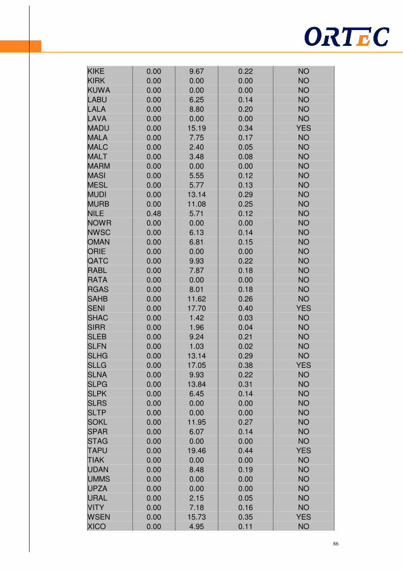
86
86
KIKE 0.00 9.67 0.22 NO
KIRK 0.00 0.00 0.00 NO
KUWA 0.00 0.00 0.00 NO
LABU 0.00 6.25 0.14 NO
LALA 0.00 8.80 0.20 NO
LAVA 0.00 0.00 0.00 NO
MADU 0.00 15.19 0.34 YES
MALA 0.00 7.75 0.17 NO
MALC 0.00 2.40 0.05 NO
MALT 0.00 3.48 0.08 NO
MARM 0.00 0.00 0.00 NO
MASI 0.00 5.55 0.12 NO
MESL 0.00 5.77 0.13 NO
MUDI 0.00 13.14 0.29 NO
MURB 0.00 11.08 0.25 NO
NILE 0.48 5.71 0.12 NO
NOWR 0.00 0.00 0.00 NO
NWSC 0.00 6.13 0.14 NO
OMAN 0.00 6.81 0.15 NO
ORIE 0.00 0.00 0.00 NO
QATC 0.00 9.93 0.22 NO
RABL 0.00 7.87 0.18 NO
RATA 0.00 0.00 0.00 NO
RGAS 0.00 8.01 0.18 NO
SAHB 0.00 11.62 0.26 NO
SENI 0.00 17.70 0.40 YES
SHAC 0.00 1.42 0.03 NO
SIRR 0.00 1.96 0.04 NO
SLEB 0.00 9.24 0.21 NO
SLFN 0.00 1.03 0.02 NO
SLHG 0.00 13.14 0.29 NO
SLLG 0.00 17.05 0.38 YES
SLNA 0.00 9.93 0.22 NO
SLPG 0.00 13.84 0.31 NO
SLPK 0.00 6.45 0.14 NO
SLRS 0.00 0.00 0.00 NO
SLTP 0.00 0.00 0.00 NO
SOKL 0.00 11.95 0.27 NO
SPAR 0.00 6.07 0.14 NO
STAG 0.00 0.00 0.00 NO
TAPU 0.00 19.46 0.44 YES
TIAK 0.00 0.00 0.00 NO
UDAN 0.00 8.48 0.19 NO
UMMS 0.00 0.00 0.00 NO
UPZA 0.00 0.00 0.00 NO
URAL 0.00 2.15 0.05 NO
VITY 0.00 7.18 0.16 NO
WSEN 0.00 15.73 0.35 YES
XICO 0.00 4.95 0.11 NO
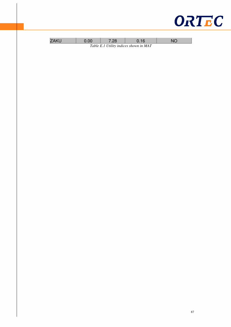
87
87
ZAKU 0.00 7.28 0.16 NO Table E.1 Utility indices shown in MAT

88
88
Appendix F – Current implementation
The algorithm described in Section 7.3.2 has been implemented in the Marginal Analysis Tool, to simplify the procedure for the user. The current contents of the upgraded MAT are:
• The minimum and maximum allowed purchase amounts are automatically adjusted for the new cases by pressing the ‘Prepare Feedstock Analysis’ button.
• The values of BASEX and MAXX , obtained by Ranging Analysis in PIMS, are
shown in the sheet ‘Feedstock Analysis’ in MAT. Also the utility indices are automatically calculated for all crude oils in Set 3.
• The user can specify an absolute or relative selection criterion for deciding which crude oils in Set 3 seem appropriate enough to displace the crude oils in Set 2 and thus for which a new case has to be prepared.
• Cases are automatically prepared (as in Table 7.2) for those crude oils that are, according to the user, appropriate (i.e. flexible) enough.
Points to improve of the Marginal Analysis Tool with Ranging Analysis:
• The user has to start Ranging Analysis in PIMS manually at this moment. Starting this procedure automatically would be an improvement for the user.
• At this moment, the time of running the complete procedure has not been reduced when using the new method (Ranging Analysis in combination with MAT), instead of running the current method (running all possible cases). Although the number of cases to be run has been reduced, the time required for running Ranging Analysis to obtain the utility indices is large, such that the complete time is approximately equal. Note that version 15.28 of PIMS is used in this thesis and Ranging Analysis may become less time-consuming in newer versions.

89
89
Outline:
Sub PrepareFACase_click()
Dim ll_row As Long
Dim li_Col As Integer
Dim li_count As Integer
Dim li_BaseTier As Integer
Dim li_BaseLocation As Integer
Dim li_BaseAct As Integer
Dim li_BasePrice As Integer
Dim li_BaseMaterType As Integer
Dim li_BaseMaterLabel As Integer
Dim li_i As Integer
Dim li_Row As Integer
Dim lb_notinbasecase As Boolean
Dim lv_basecrudes() As Variant
Dim li_count2 As Integer
Call ProcPreparePlanStar
Application.ScreenUpdating = False
Call ReadControlParameters
Call ReadModeInformation
Application.ScreenUpdating = False
Application.StatusBar = "Creating Commtrns Cargo Analysis..."
gs_LastCrudeCombination = ""
gd_Offset = Range("Offset_Cargo").value
ThisWorkbook.Worksheets("CA Crude").Activate
Application.StatusBar = "Creating Commtrns Cargo Analysis..."
gs_LastCrudeCombination = ""
gd_Offset = Range("Offset_Cargo").value
ThisWorkbook.Worksheets(gs_CargoInput_Crude).Activate
gi_col_commtrns_RHS = Application.WorksheetFunction.Match("RHS", Rows(1), 0)
gi_col_commtrns_Location = Application.WorksheetFunction.Match("LOCATION", Rows(1), 0)
gi_col_commtrns_MaterLabel = Application.WorksheetFunction.Match("CRUDE", Rows(1), 0)
gi_col_commtrns_Tier = Application.WorksheetFunction.Match("TIER", Rows(1), 0)
gi_col_commtrns_Price = Application.WorksheetFunction.Match("PRICE", Rows(1), 0)
gi_col_commtrns_BaseCaseCrude = Application.WorksheetFunction.Match("BASE_MATERLABEL",
Rows(1), 0)
gi_col_commtrns_BaseCaseLocation = Application.WorksheetFunction.Match("BASELOCATION",
Rows(1), 0)
gi_col_commtrns_BaseCrude = Application.WorksheetFunction.Match("BASE_CRUDE", Rows(1), 0)
gi_col_commtrns_MIN = Application.WorksheetFunction.Match("MIN_BASE", Rows(1), 0)
gi_col_commtrns_MAX = Application.WorksheetFunction.Match("MAX_BASE", Rows(1), 0)
gi_col_commtrns_Actual = Application.WorksheetFunction.Match("ACT_BASE", Rows(1), 0)
gi_col_commtrns_BaseCase = Application.WorksheetFunction.Match("BASECASE", Rows(1), 0)

90
90
gi_col_commtrns_MINcorr = Application.WorksheetFunction.Match("MIN_CORR", Rows(1), 0)
gi_col_commtrns_MAXcorr = Application.WorksheetFunction.Match("MAX_CORR", Rows(1), 0)
gi_col_commtrns_Active = Application.WorksheetFunction.Match("ACTIVE", Rows(1), 0)
Call Empty_commtrns
' 'Set variables that do not change
c_commtrns_Version = Range("modelid1")
c_commtrns_Currency = Range("currency").value
c_commtrns_FOBPrice = "N"
c_commtrns_OrderNr = "1"
c_commtrns_TransType = "IMP"
c_commtrns_MaterType = "CRUDE"
c_commtrns_QtyUOM = Range("Uom_Quant").value
c_commtrns_PriceUOM = c_commtrns_QtyUOM
gd_first_drop_quantity = Range("first_drop_quantity")
c_commtrns_Period = Range("PeriodOutput")
'Check all base_cases that are fixed in a mode and fix them in the base cases
'this is for both crudes and feedstocks!
ls_sheet = "CA Crude"
ll_row = gl_row_input_start
ThisWorkbook.Worksheets(ls_sheet).Activate
li_BaseTier = Application.WorksheetFunction.Match("BASETIER", Rows(1), 0)
li_BaseLocation = Application.WorksheetFunction.Match("BASELOCATION", Rows(1), 0)
li_BaseAct = Application.WorksheetFunction.Match("BASE_ACT", Rows(1), 0)
li_BasePrice = Application.WorksheetFunction.Match("BASEPRICE", Rows(1), 0)
li_BaseMaterType = Application.WorksheetFunction.Match("BASE_MATERTYPE", Rows(1), 0)
li_BaseMaterLabel = Application.WorksheetFunction.Match("BASE_MATERLABEL", Rows(1), 0)
With Sheets(ls_sheet)
Do While .Cells(ll_row, gi_col_commtrns_BaseCaseCrude) <> ""
For li_i = 1 To gl_nrModes
If gc_ModesCollection(li_i).tb_crude Then
ReDim Preserve lv_basecrudes(ll_row - 13)
lv_basecrudes(ll_row - 13) = .Cells(ll_row, li_BaseMaterLabel)
If gc_ModesCollection(li_i).tb_active Then 'only export if mode is active
If .Cells(ll_row, gc_ModesCollection(li_i).tl_column) <> "" Then 'crude is fixed for this
mode
c_commtrns_Location = .Cells(ll_row, li_BaseLocation)
c_commtrns_MaterType = .Cells(ll_row, li_BaseMaterType)
c_commtrns_MaterLabel = .Cells(ll_row, li_BaseMaterLabel)
c_commtrns_Qty_Min = .Cells(ll_row, li_BaseAct)
c_commtrns_Tier = .Cells(ll_row, li_BaseTier)
c_commtrns_Price = .Cells(ll_row, li_BasePrice)
91
91
c_commtrns_Qty_Max = .Cells(ll_row, li_BaseAct)
c_commtrns_Rhs = gc_ModesCollection(li_i).ts_rhs
c_commtrns_Dmn = "BASIC"
Call AddTo_commtrns_List
If gb_MPmodel Then
c_commtrns_Dmn = "GLOBAL"
Call AddTo_commtrns_List
End If
Else 'crude is not fixed for this mode
c_commtrns_Location = .Cells(ll_row, li_BaseLocation)
c_commtrns_MaterType = .Cells(ll_row, li_BaseMaterType)
c_commtrns_MaterLabel = .Cells(ll_row, li_BaseMaterLabel)
c_commtrns_Qty_Min = 0 'min is always zero when crude is not fixed
c_commtrns_Tier = .Cells(ll_row, li_BaseTier)
c_commtrns_Price = .Cells(ll_row, li_BasePrice)
If .Cells(ll_row, 41) = 0 Then
c_commtrns_Qty_Max = 9999 'if crude is not fixed and max=0
Else
c_commtrns_Qty_Max = .Cells(ll_row, 41)
End If
c_commtrns_Rhs = gc_ModesCollection(li_i).ts_rhs
c_commtrns_Dmn = "BASIC"
Call AddTo_commtrns_List
If gb_MPmodel Then
c_commtrns_Dmn = "GLOBAL"
Call AddTo_commtrns_List
End If
End If
End If
End If
Next li_i
ll_row = ll_row + 1
Loop
End With
li_Row = 6
While Sheets("comp_label_crudes").Cells(li_Row, 3) <> ""
lb_notinbasecase = True
li_count2 = 0
While (li_count2 <> ll_row - 13) And (lb_notinbasecase = True)
If Sheets("comp_label_crudes").Cells(li_Row, 3) = lv_basecrudes(li_count2) Then 'is the crude in
comp_label_crudes in the base case??
lb_notinbasecase = False
End If
li_count2 = li_count2 + 1
Wend
If lb_notinbasecase Then 'if not in base case, min=0, max=9999
c_commtrns_Location = Range("location")
c_commtrns_MaterType = "CRUDE"
92
92
c_commtrns_MaterLabel = Sheets("comp_label_crudes").Cells(li_Row, 3)
c_commtrns_Qty_Min = 0
c_commtrns_Tier = 1
c_commtrns_Price = 75
c_commtrns_Qty_Max = 9999
c_commtrns_Rhs = "M100"
c_commtrns_Dmn = "BASIC"
Call AddTo_commtrns_List
If gb_MPmodel Then
c_commtrns_Dmn = "GLOBAL"
Call AddTo_commtrns_List
End If
End If
li_Row = li_Row + 1
Wend
Call Write_commtrns_ToSheet
Call SaveOneSheet(Range("directory"), "commtrns")
Application.StatusBar = False
Application.ScreenUpdating = True
Sheets("General").Activate
End Sub
Sub FeedstockAnalysis()
Dim as_planstar_basecase_outputdir As String
Dim as_runid_dir_manual As String
Dim ADOConnection As ADODB.Connection
Dim ADORS As ADODB.Recordset
Dim ADOConnectionString As String
Dim RowCounter As Long
Dim lws_FASheet As Worksheet
Dim lws_GeneralSheet As Worksheet
Dim ls_VBName As String
Dim li_count As Integer
Dim li_count2 As Integer
Dim ls_crudes() As Variant
Dim ls_crudes2 As String
Dim ls_crudes2cut() As String
Dim lv_query As Variant
Dim ls_sheet As String
Dim li_length As Integer
Dim ls_RangeCase As String
Dim ls_VariableName As String
Dim ll_VariableValue As Double
Dim ls_name As String
Dim li_NumberCrudes As Integer
93
93
Dim li_loop As Integer
Dim li_CrudeNumber As Integer
Dim li_cases As Integer
Dim gs_connection As String
Dim ld_totalfeed As Double
On Error GoTo errorhandler
'Application.ScreenUpdating = False
as_planstar_basecase_outputdir = Left(Range("planstar_basecase_outputdir"),
Len(Range("planstar_basecase_outputdir")) - 8 - Len(Range("location"))) & "Run_10\" &
Range("location") & "\"
as_runid_dir_manual = Left(Range("planstar_basecase_outputdir"),
Len(Range("planstar_basecase_outputdir")) - 8 - Len(Range("location"))) & "Run_10\" &
Range("location") & "\Manual\"
gs_connection = "ODBC;DSN=" + Range("dsn") + ";UID=hia;PWD=hia"
'-------AB: Pick up the FA values from results.mdb -------
Sheets("CA Crude").Activate
'Build an ADO connection string for the database to be queried
ADOConnectionString = BuildADOConnectionString(as_planstar_basecase_outputdir & "Results.mdb")
If ADOConnectionString = "" Then
Exit Sub
End If
'Open the ADO connection
If OpenADODatabaseConnection(ADOConnection, ADOConnectionString, False) = False Then
GoTo SubExit
End If
'create a new workbook with the right name: FeedstockAnalysis.xls (ipv BaseExpertBounds.xls)
Call DeleteBook(as_runid_dir_manual & "FeedstockAnalysis.xls")
Workbooks.Add
ActiveSheet.name = "FEEDSTOCKANALYSIS"
Set lws_FASheet = ActiveWorkbook.Sheets("FEEDSTOCKANALYSIS")
ls_VBName = ActiveWorkbook.name
'insert the first row with the column headers
Range("A1").Select
Cells(1, 1) = "Range Case"
Cells(1, 2) = "Variable Name"
Cells(1, 3) = "Value"
'Open a recordset for the table
If OpenADORecordSet(ADOConnection, ADORS, "SELECT PrFeedstockRange.RangeCase,
PrFeedstockRange.VariableName, PrFeedstockRange.VariableValue FROM PrFeedstockRange INNER
JOIN PRSolutionID on PRFeedstockRange.SolutionID=PRSolutionID.SolutionID order by
PrFeedstockRange.RangeCase, PrFeedstockRange.VariableName") = False Then

94
94
GoTo SubExit
End If
'Loop through the returned records one row at a time to return the data
li_NumberCrudes = 0
RowCounter = 2
li_count = 0
ReDim ls_crudes(0)
With ADORS
While Not .EOF
ls_RangeCase = .Fields(0).value
ls_VariableName = .Fields(1).value
ll_VariableValue = .Fields(2).value
lws_FASheet.Cells(RowCounter, 1).value = ls_RangeCase
lws_FASheet.Cells(RowCounter, 2).value = ls_VariableName
lws_FASheet.Cells(RowCounter, 3).value = ll_VariableValue
If RowCounter = 2 Then
ls_crudes(0) = ls_VariableName
ls_crudes2 = "('" & ls_VariableName & "', "
li_CrudeNumber = 1
'AB: adding PS name
lws_FASheet.Cells(1, 7) = ls_VariableName
lv_query = Array( _
"select hcl_complabel from complabel_mapping where mapping_id='east' and
naming_convention='PIMS' and complabel='" & ls_VariableName & "'")
'AB: mapping_id is hardcoded (2 keer)
With ActiveSheet.QueryTables.Add(Connection:=gs_connection, Destination:=Cells(1, 8))
.CommandText = lv_query
.FieldNames = False
.name = "query_table_FeedstockAnalysis"
ls_name = .name
End With
With ActiveSheet.QueryTables(ls_name)
.PreserveFormatting = True
.RefreshStyle = xlOverwriteCells
.Refresh BackgroundQuery:=False
End With
Call SetQueryTableOptions("FEEDSTOCKANALYSIS", ls_name)
ThisWorkbook.Names.Add name:="Fixed_Crudes", RefersTo:=Names("FEEDSTOCKANALYSIS" +
"!" + ls_name).RefersTo
Else
For li_loop = 0 To li_NumberCrudes
If (ls_VariableName = ls_crudes(li_loop)) Then
li_CrudeNumber = li_loop + 1
GoTo AlreadyAddedbefore
End If
Next

95
95
ReDim Preserve ls_crudes(li_NumberCrudes + 1)
ls_crudes(li_NumberCrudes + 1) = ls_VariableName
lws_FASheet.Cells(li_NumberCrudes + 2, 7) = ls_VariableName
li_NumberCrudes = li_NumberCrudes + 1
li_CrudeNumber = li_NumberCrudes + 1
ls_crudes2 = ls_crudes2 & "'" & ls_VariableName & "'" & ", "
lv_query = Array( _
"select hcl_complabel from complabel_mapping where mapping_id='east' and
naming_convention='PIMS' and complabel='" & ls_VariableName & "'") 'hardcoded
With ActiveSheet.QueryTables.Add(Connection:=gs_connection,
Destination:=Cells(li_NumberCrudes + 1, 8))
.CommandText = lv_query
.FieldNames = False
.name = "query_table_FeedstockAnalysis"
ls_name = .name
End With
With ActiveSheet.QueryTables(ls_name)
.PreserveFormatting = True
.RefreshStyle = xlOverwriteCells
.Refresh BackgroundQuery:=False
End With
Call SetQueryTableOptions("FEEDSTOCKANALYSIS", ls_name)
ThisWorkbook.Names.Add name:="Fixed_Crudes", RefersTo:=Names("FEEDSTOCKANALYSIS" +
"!" + ls_name).RefersTo
End If
AlreadyAddedbefore:
If (lws_FASheet.Cells(RowCounter, 1) = "!Base") Then
ld_totalfeed = ld_totalfeed + ll_VariableValue
lws_FASheet.Cells(li_CrudeNumber, 9) = ll_VariableValue
ElseIf (lws_FASheet.Cells(RowCounter, 1) = ls_VariableName & "MAX") Then
lws_FASheet.Cells(li_CrudeNumber, 10) = ll_VariableValue
End If
.MoveNext
RowCounter = RowCounter + 1
Wend
End With
li_length = Len(ls_crudes2)
Mid(ls_crudes2, li_length - 1) = ")"
For i = 1 To (li_NumberCrudes + 1)
If Cells(i, 9) = "" Then
Cells(i, 9) = Application.WorksheetFunction.VLookup(Cells(i, 7), Range("B1:C" & li_NumberCrudes
+ 2), 2, False)
End If
If Cells(i, 10) = "" Then
Cells(i, 10) = Application.WorksheetFunction.VLookup(Cells(i, 7), Range("B1:C" & li_NumberCrudes
+ 2), 2, False)
End If

96
96
Next
'---------AB: Calculate utility indices for the crudes--------
For li_count2 = 0 To li_NumberCrudes
If lws_FASheet.Cells(li_count2 + 1, 10) = "" Then
lws_FASheet.Cells(li_count2 + 1, 11) = 0
lws_FASheet.Cells(li_count2 + 1, 10) = lws_FASheet.Cells(li_count2 + 1, 9)
Else
lws_FASheet.Cells(li_count2 + 1, 11) = (lws_FASheet.Cells(li_count2 + 1, 10) / ld_totalfeed -
lws_FASheet.Cells(li_count2 + 1, 9) / ld_totalfeed) / (1 - lws_FASheet.Cells(li_count2 + 1, 9) / ld_totalfeed)
End If
Next
lws_FASheet.Columns("G:K").Select
Selection.Copy
Application.DisplayAlerts = False
ActiveWorkbook.Close
Application.DisplayAlerts = True
'---------AB: Write Xmax-Xmin with corresponding crudes in FA Sheet------
Sheets("Feedstock Analysis").Activate
ActiveSheet.Range("A2:E300").ClearContents
'---------AB: Prepare appropriate cases in CA Crude sheet----------
Range("A2").Select
Selection.PasteSpecial
li_cases = 13
Sheets("CA Crude").Range("N13:O300").ClearContents
Sheets("CA Crude").Range("Q13:Q300").ClearContents
Sheets("CA Crude").Range("S13:S300").ClearContents
Sheets("CA Crude").Range("U13:X300").ClearContents
Sheets("CA Crude").Range("AA13:AA300").ClearContents
For li_count = 2 To (li_NumberCrudes + 2)
If Sheets("Feedstock Analysis").Cells(li_count, 6) = "YES" Then
Sheets("CA Crude").Cells(li_cases, 14) = Range("location")
Sheets("CA Crude").Cells(li_cases, 15) = Sheets("Feedstock Analysis").Cells(li_count, 2)
Sheets("CA Crude").Cells(li_cases, 17) = 1
Sheets("CA Crude").Cells(li_cases, 19) = "Y"
Sheets("CA Crude").Cells(li_cases, 24) = 80
Sheets("CA Crude").Cells(li_cases, 27) = "H"
li_cases = li_cases + 1
End If
Next
Exit Sub
SubExit:

97
97
'Make sure the ADO recordset is closed
If Not ADORS Is Nothing Then
ADORS.Close
End If
'Make sure the ADO connection is closed
If Not ADOConnection Is Nothing Then
ADOConnection.Close
End If
'Clear object memory
Set ADORS = Nothing
Set ADOConnection = Nothing
Set lws_BoundsSheet = Nothing
Set lws_CapsSheet = Nothing
Set lws_GeneralSheet = Nothing
errorhandler:
Application.ScreenUpdating = True
MsgBox "Error " & Err & ": " & Error$ & " occurred."
Application.DisplayAlerts = False
ActiveWorkbook.Close
Application.DisplayAlerts = True
End Sub
Sub Abs_criterion()
Dim ls_value As String
Dim i As Integer
If Worksheets("General").OptionButton1.value = True Then
ls_value = Worksheets("General").TextBox1.value
If ls_value = "" Then
Exit Sub
End If
Sheets("Feedstock Analysis").Range("F2:F300").FormulaR1C1 = "=IF(RC5="""","""",IF(RC5>" &
ls_value & ",""YES"",""NO""))"
End If
End Sub
Sub Rel_criterion()
Dim ls_value As String
Dim i As Integer
If Worksheets("General").OptionButton2.value = True Then
ls_value = Worksheets("General").TextBox2.value
If ls_value = "" Then

98
98
Exit Sub
End If
Sheets("Feedstock Analysis").Range("F2:F300").FormulaR1C1 =
"=IF(RC5="""","""",IF(RANK(RC5,C5)/(COUNT(C5)-1)<=0.01*" & ls_value & ",""YES"",""NO""))"
End If
End Sub

99
99
Appendix G – Outcomes of Example 8
Refinery Y Refinery Z Crude oil Rank CIV's Rank utility Crude oil Rank CIV's Rank utility
indices indices
STAG 1 73 DOBA 1 56
SLPG 2 71 DURI 2 63
MIRI 3 64 NILE 3 52
AGTL 4 34 STAG 4 69
KUIT 5 103 UDAN 5 31
ZUAS 6 28 CABD 6 41
QINH 7 114 AMNA 7 32
THEV 8 16 LALA 8 27
ANGS 9 14 BAHO 9 30
ALSH 10 38 RABL 10 35
SLEB 11 66 GIRA 11 44
BARR 12 41 KIKE 12 22
XIJI 13 85 FORC 13 49
YOMB 14 112 KEKW 14 8
VITY 15 50 CANU 15 59
EACR 16 45 ERHA 16 42
RABL 17 76 LABU 17 46
SOKL 18 75 BENC 18 29
WALI 19 106 MARM 19 69
FORC 20 94 BONL 20 33
DOBA 21 108 XICO 22 54
MARM 22 9 CHEX 23 55
ESPO 23 67 SLEB 24 24
BINT 24 60 MUDI 25 13
NALT 25 53 JATI 26 60
OMAN 26 35 KAJI 27 23
KEKW 27 32 MASI 28 51
ZHAD 28 113 ANGS 29 5
RASB 29 39 SOKL 30 15
CEND 30 17 VITY 31 40
ENFI 31 95 MALA 32 36
DURI 32 111 WSEN 33 6
QARU 33 116 TAPU 34 1
RABB 34 37 BREB 35 37
NILE 35 78 KIDU 36 26
MUTI 36 2 ARJU 37 11
PUF7 37 31 SAHB 38 16
RATA 38 18 BRNL 39 9
ARAH 39 5 MURB 40 17
BNGA 40 59 HAND 41 19

100
100
MINA 41 98 ORIE 42 69
PENL 42 84 OMAN 43 43
KIKE 43 24 URAL 44 64
UDAN 44 69 COSB 45 25
RANG 45 44 ARXL 46 28
JATI 46 80 ARSL 47 38
KUWA 47 13 ZAKU 48 39
LEGE 48 25 MALT 49 58
ARJU 49 57 MADU 50 7
QATL 50 42 SENI 51 2
URAL 51 97 QATC 52 21
ZAKU 52 62 GULS 53 69
SUTU 53 82 IRNL 54 66
CHEX 54 52 RGAS 55 34
DAIH 55 20 MESL 56 50
LUFE 56 87 TIAK 58 69
GERA 57 26 SPAR 59 48
SLPH 58 115 KHUF 60 14
LANG 59 19 LAVA 61 69
MASI 60 40 SIRR 62 65
UMMS 61 70 BINC 63 69
NKOS 62 91 ARUN 64 18
BONL 63 88 KATA 65 4
KIDU 64 65 HOUT 66 69
IRNL 65 79 ESPA 67 61
M100 66 36 IRNH 68 69
DUBA 67 8 MALC 69 62
CYRU 68 1 UPZA 70 69
KUMK 69 54 NWSC 71 47
HAND 70 83 CAKE 72 53
CINT 71 96 SHAC 73 67
BASK 72 43 KIRK 74 69
ORIE 73 4 BASL 75 69
BUAT 74 29 ARAM 76 69
IRNH 75 48 KUWA 77 69
TAPU 76 58 ARAH 78 69
QATM 77 47 KHAF 79 69
KERA 78 110 RATA 80 69
BEKA 79 107 CYRU 81 69
SARI 80 100 NOWR 82 69
KAJI 81 86 IBMS 83 69
SLPK 82 77 SLRS 84 69
MUDI 83 68 BUKN 85 69
KHAF 84 3 SLNA 86 20
TUIO 85 55 SLFN 87 68
ANOA 86 104 SLTP 88 69
SENI 87 10 SLPK 89 45
EOCE 88 102 SLHG 90 12
LSFO 89 117 SLPG 91 10
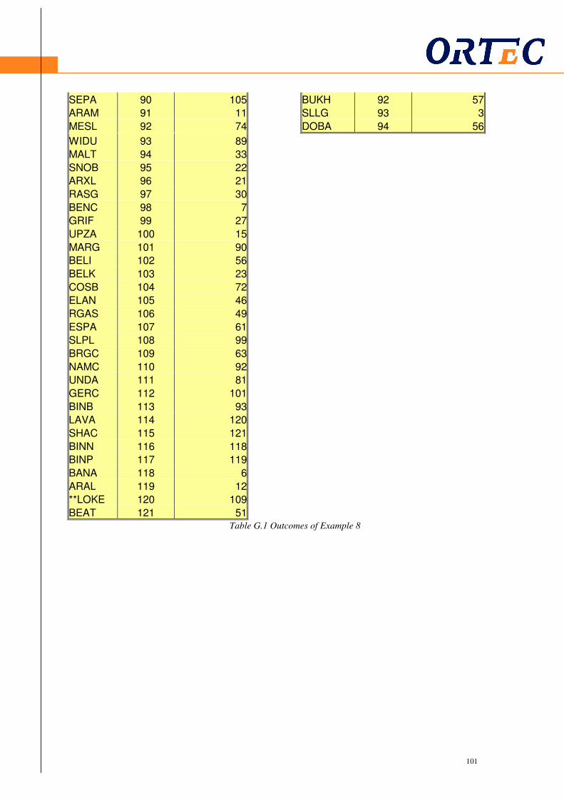
101
101
SEPA 90 105 BUKH 92 57
ARAM 91 11 SLLG 93 3
MESL 92 74 DOBA 94 56
WIDU 93 89
MALT 94 33
SNOB 95 22
ARXL 96 21
RASG 97 30
BENC 98 7
GRIF 99 27
UPZA 100 15
MARG 101 90
BELI 102 56
BELK 103 23
COSB 104 72
ELAN 105 46
RGAS 106 49
ESPA 107 61
SLPL 108 99
BRGC 109 63
NAMC 110 92
UNDA 111 81
GERC 112 101
BINB 113 93
LAVA 114 120
SHAC 115 121
BINN 116 118
BINP 117 119
BANA 118 6
ARAL 119 12
**LOKE 120 109
BEAT 121 51Table G.1 Outcomes of Example 8