Solvable Affine Term Structure Models

Martino Grasselli and Claudio TebaldiUniversità degli Studi di Verona ∗

May 7, 2004

Abstract

Pricing of contingent claims in the Affine Term Structure Mod-els (ATSM) can be reduced to the solution of a set of Riccati-typeOrdinary Differential Equations (ODE), as shown in Duffie, Pan andSingleton (2000) and in Duffie, Filipovic and Schachermayer (2001).We discuss the solvability of these equations. While admissibility is anecessary and sufficient condition in order to express their general so-lution as an analytic series expansion, we prove that, when the factorsare restricted to have continuous paths, these ODE admit a funda-mental system of solutions if and only if all the positive factors are in-dependent. Finally, we classify and solve all the consistent polynomialterm structure models admitting a fundamental system of solutions.

Keywords: Affine Terms Structure Models, Riccati ODE, Lie algebra,Fundamental System of Solutions.

1 Introduction

The class of multifactor Affine Term Structure Models (ATSM hereafter)as introduced by Duffie and Kan (1996), combines some financial appealingproperties:

1. The sensitivities of the zero coupon yield curve to the stochastic factorsare deterministic, as discussed in Brown and Schaefer (1994);

∗Department of Economics, Via Giardino Giusti 2, 37129 Verona, Italy. Fax +390458054935. E-mail: martino.grasselli@univr.it, claudio.tebaldi@univr.it

1

2. Explicit parametric restrictions, called admissibility conditions, grantthe existence of a regular affine process, as discussed in Dai and Sin-gleton (2000) and in Duffie, Filipovic and Schachermayer (2001); inparticular correlations between positive factors are allowed.

3. The pricing problem can be reduced to the solution of a system ofODE as discussed in Duffie, Pan and Singleton (2000). In fact, theexplicit expression of the conditional discounted characteristic functionof the factors can be specified in terms of the solutions of (deterministic)Riccati equations for any admissible ATSM (see e.g. Duffie et al. 2001).

In this paper we discuss the solvability of such Riccati ODE. Althoughthey have been well discussed and classified in many books (see e.g. Reid1972), in the multi dimensional context most of the interest has been devotedto a particular subset called Matrix Riccati ODE, which are completely inte-grable. Unfortunately, Riccati ODE arising within admissible ATSM do notbelong to this class in general.We provide a systematic classification of the necessary and sufficient con-

ditions in order to obtaini) an analytic series solutionii) a Fundamental System of Solution (FSS), i.e. a closed form expression

in terms of a finite number of parameters.In particular, we find that when the factors are restricted to have contin-

uous paths, the existence of a FSS is in contradiction with the presence ofcorrelations between positive factors. Finally, extending the above analysis,we provide a systematic classification and solution of all general polynomialterm structure models which admit a FSS.The paper is organized as follows: in Section 2 we introduce the pricing

problem in ATSM and we discuss a reduced normal form togheter with theadmissibility issue. In Section 3 we show that the admissibility of the ATSMimplies that the series expansion solution is analytic, we compute explicitlythe series coefficients and we discuss the necessary and sufficient parametricrestrictions for the Riccati ODE in order to admit a FSS. Finally we findthe explicit solution for all consistent separable polynomial term structures.In Appendix A we review two approaches in the simplest one-dimensionalcase, while Appendix B shows an example of ”quasi closed form” solution forATSM not admitting a FSS.

2

2 Stochastic dynamics of factors and the pric-ing problem

The specification of an ATSM can be given in full generality even in presenceof jump diffusion processes according to the approach of Duffie et al. (2001).Here we restrict our treatment to the more familiar setup of Duffie and Kan(1996) model in the specification proposed in Dai and Singleton (2000), whichis essentially the same of Duffie, Pan and Singleton (2000) model when factorsare restricted to have continuous paths. This restriction is adopted in orderto simplify the exposition and to disclose the applicative follow-up of theabove general results within the more traditional notation and frameworkfor financial applications.

Definition 1 A Term Structure Model is Affine (ATSM) if the short interestrate rt is an affine combination of factors

rt = δ0 + δ0Yt, t ≥ 0

for some δ0 ∈ R and δ ∈ Rn, and the dynamics of the factors under the riskneutral measure Q satisfies the following SDE:

dYt = K (θ − Yt) dt+ Σdiagh(αi + β0iYt)

1/2idWt, t ≥ 0, (1)

Y0 = y ∈ Rn,

where Wt is an n-dimensional standard Brownian motion and

θ, α ∈ Rn,

K, β ∈ Mn,

Σ ∈ GLn

where αi indicates the i− th element of the vector α, βi indicates the i− thcolumn of matrix β, and given a vector z ∈ Rn, diag (zi) ∈Mn is the diagonalmatrix with the elements of the vector z along the diagonal (the prime 0

denotes transposition). Σ is required to be invertible as in Duffie and Kan(1996) excluding the presence of deterministic factors.

The rank of β is defined to be tom ≤ n: in the notation of Dai and Single-ton (2000),m classifies the families Am (n) of admissible models parametrizedby m,n. Without loss of generality we assume that the upper left minor oforder m is non singular.

3

Being interested in pricing contingent claims, we follow Duffie, Pan andSingleton (2000) and compute the discounted characteristic function of thefactors Yt, conditional on the information at time t ≤ T :

ΨY (v, Yt, t, T ) = Et·exp

µ−Z T

t

r (s) ds

¶exp (v0YT )

¸, v ∈ Cn.

Under technical integrability conditions, Duffie, Pan and Singleton (2000)have shown that the previous function can be explicitly written as an expo-nential affine function of the factors:

ΨY (v, Yt, t, T ) = exp¡A (t) + B (t)0 Yt¢ , t ≤ T, (2)

where A ∈ C,B ∈ Cn satisfy the following complex-valued backward ODE

− d

dtB(t) = −K0B(t) + 1

2

nXi=1

[(Σ0B(t))i]2 βi − δ, (3)

− d

dtA(t) = −θK0B(t) + 1

2

nXi=1

[(Σ0B(t))i]2 αi − δ0,

with boundary conditions

B(T ) = v,

A(T ) = 0.

Remark 1 An important contingent claim is the zero-coupon bond, whoseprice is given by (t ≤ T )

P (t, T ) = Et·exp

µ−Z T

t

r (s) ds

¶¸= exp (A (t) + B (t)Yt) ,

where A,B satisfy eq.s (3) with boundary conditionsB(T ) = 0,

A(T ) = 0.

When dealing with bonds, the sensitivities A,B are usually expressed as func-tions of time to maturity: τ = T − t. In fact when parameters are timeindependent, prices depend only on the combination τ = T − t and RiccatiODE become a genuine initial value problem at τ = 0. Under the change ofvariables t→ τ the left hand side of eq.(3) gets a factor −1.

4

Remark 2 An alternative way to define the ATSM consists in requiringthat the characteristic function in eq.(2) has the exponential affine form asin Duffie et al. (2001).

Remark 3 In the alternative approach of Elliott and van der Hoek (2001),it is shown that the solution of the Riccati (3) can be expressed through theexpected value, under the forward measure, of the stochastic Jacobian, andsuch expected value turns out to be deterministic for ATSM. As discussedin Grasselli and Tebaldi (2004), however, this approach applied to multifac-tor ATSM leads to a non linear equation which is equivalent and perfectlyconsistent with our algebraic results when dealing with the solvability issue.

2.1 Symmetry reduction and Normal Form for ATSM

Each ATSM is identified by the following vector of parameters (δ0, δ, K, θ,Σ, αi, βi1≤i≤n). As discussed in Dai and Singleton (2000), an affine changeof variables:

Y → X = LY + ϑ L ∈ GLn, ϑ ∈ Rn (4)

leaves unaffected all the prices, while the parameters are changed accordingto:

(δ0, δ,K, θ,Σ, αi, βi1≤i≤n)→(δ0−δ0L−1ϑ, ¡L−1¢0 δ, LKL−1, Lθ+ϑ,L−1Σ,©¡α− β0L−1ϑ

¢i,¡β0L−1

¢i

ª1≤i≤n)

It is thus possible to reduce the discussion of a whole class of models, thosediffering at most for an affine change of variables, to a single representativeelement which we will call hereafter normal form.Let us now discuss the change of variables that relates a generic ATSM

with the corresponding normal form.

Definition 2 (Normal Form) Consider a symmetry transformation (L, ϑ)of the type given in eq.(4). Let us fix L = Σ−1 and ϑ ∈ Rn any solution tothe system of equations

β0iΣϑ = αi, i = 1, ..,m,©Σ−1K (θ − ϑ)

ªi= 0, i = m+ 1, .., n.

Such a transformation maps the original factors’ dynamics (1) into the Nor-mal Form ATSM, whose factors’ dynamics becomes

dXt =¡AXt +A0

¢dt+ diag

hS1/2ii

idWt, t ≥ 0, (5)

Sii =¡CiXt + C0

i

¢,

X0 = x,

5

(Ci denotes the i − th row of the matrix C, m = rank (C)) while the shortrate is given by

rt = γ0 + γ0Xt,

where the parameters φ = (γ, γ0, A,A0, C,C0)are defined as follows:

Xt = Σ−1Yt, t ≥ 0,γ0 = δ0 − δ0Σϑ,γ = Σ0δ,

A = −Σ−1KΣ ∈Mn,

A0 = Σ−1K (θ − ϑ) ∈ Rn,

C = β0Σ ∈Mn,

C0 = α− β0Σϑ,

where (C0)i = 0, i = 1, ..,m and (A0)i = 0, i = m+ 1, .., n

The Riccati ODE providing the generalized conditional characteristicfunction

ΨX (u,Xt, t, T ) = exp¡V0 (t) + V (t)0Xt

¢, t ≤ T,

u = Σv

become (i = 1, ..n):

− d

dtVi(t) =

nXj=1

(A0)ij Vj(t) +1

2

nXj=1

(C 0)ij V2j (t)− γi, V(T ) = u, (6)

− d

dtV0(t) =

nXj=1

A0jVj(t) +1

2

nXj=1

¡C0j

¢V2j (t)− γ0, V0(T ) = 0,

with

γ = Σ0δ ∈ Rn, (7)

γ0 = δ0 − δ0Σϑ ∈ R.

Remark 4 The zero-coupon bond price expression in terms of the reducedfactors will be:

P (t, T ) = exp¡V0 (t) + V 0 (t)Xt

¢(8)

Vi (T ) = 0 i = 0, .., n.

6

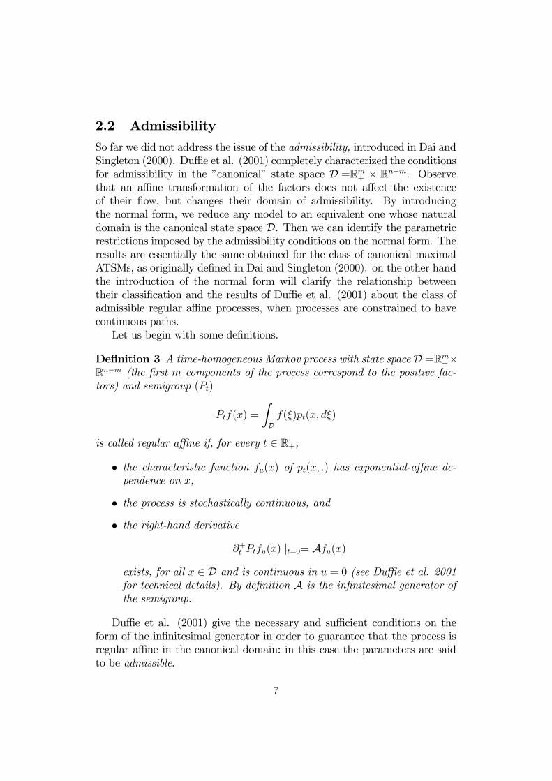
2.2 Admissibility

So far we did not address the issue of the admissibility, introduced in Dai andSingleton (2000). Duffie et al. (2001) completely characterized the conditionsfor admissibility in the ”canonical” state space D =Rm

+ × Rn−m. Observethat an affine transformation of the factors does not affect the existenceof their flow, but changes their domain of admissibility. By introducingthe normal form, we reduce any model to an equivalent one whose naturaldomain is the canonical state space D. Then we can identify the parametricrestrictions imposed by the admissibility conditions on the normal form. Theresults are essentially the same obtained for the class of canonical maximalATSMs, as originally defined in Dai and Singleton (2000): on the other handthe introduction of the normal form will clarify the relationship betweentheir classification and the results of Duffie et al. (2001) about the class ofadmissible regular affine processes, when processes are constrained to havecontinuous paths.Let us begin with some definitions.

Definition 3 A time-homogeneous Markov process with state space D =Rm+×

Rn−m (the first m components of the process correspond to the positive fac-tors) and semigroup (Pt)

Ptf(x) =

ZDf(ξ)pt(x, dξ)

is called regular affine if, for every t ∈ R+,• the characteristic function fu(x) of pt(x, .) has exponential-affine de-pendence on x,

• the process is stochastically continuous, and• the right-hand derivative

∂+t Ptfu(x) |t=0= Afu(x)exists, for all x ∈ D and is continuous in u = 0 (see Duffie et al. 2001for technical details). By definition A is the infinitesimal generator ofthe semigroup.

Duffie et al. (2001) give the necessary and sufficient conditions on theform of the infinitesimal generator in order to guarantee that the process isregular affine in the canonical domain: in this case the parameters are saidto be admissible.

7

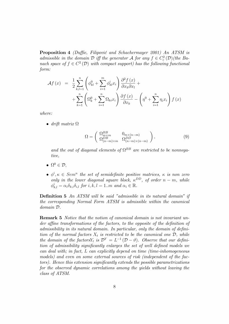
Proposition 4 (Duffie, Filipovic and Schachermayer 2001) An ATSM isadmissible in the domain D iff the generator A for any f ∈ C2

c (D)(the Ba-nach space of f ∈ C2 (D) with compact support) has the following functionalform:

Af (x) =1

2

nXk,l=1

Ãφ0kl +

mXi=1

φiklxi

!∂2f (x)

∂xk∂xl+

+nX

k=1

ÃΩ0k +

nXi=1

Ωkixi

!∂f (x)

∂xk−Ãη0 +

nXi=1

ηixi

!f (x)

where:

• drift matrix Ω

Ω =

µΩBBm×m 0m×(n−m)

ΩDB(n−m)×m ΩDD

(n−m)×(n−m)

¶, (9)

and the out of diagonal elements of ΩBB are restricted to be nonnega-tive,

• Ω0 ∈ D,• φi, κ ∈ Semn the set of semidefinite positive matrices, κ is non zeroonly in the lower diagonal square block, κDD, of order n − m, whileφik,l = αiδk,iδi,l for i, k, l = 1..m and αi ∈ R.

Definition 5 An ATSM will be said ”admissible in its natural domain” ifthe corresponding Normal Form ATSM is admissible within the canonicaldomain D.

Remark 5 Notice that the notion of canonical domain is not invariant un-der affine transformations of the factors, to the opposite of the definition ofadmissibility in its natural domain. In particular, only the domain of defini-tion of the normal factors Xt is restricted to be the canonical one D, whilethe domain of the factorsYt is DY = L−1 (D − ϑ). Observe that our defini-tion of admissibility significantly enlarges the set of well defined models wecan deal with; in fact, L can explicitly depend on time (time-inhomogeneousmodels) and even on some external sources of risk (independent of the fac-tors). Hence this extension significantly extends the possible parametrizationsfor the observed dynamic correlations among the yields without leaving theclass of ATSM.

8

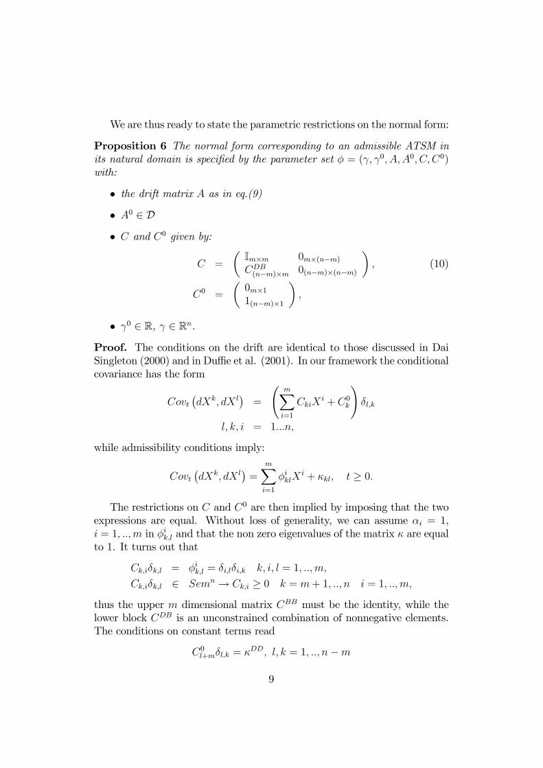
We are thus ready to state the parametric restrictions on the normal form:

Proposition 6 The normal form corresponding to an admissible ATSM inits natural domain is specified by the parameter set φ = (γ, γ0, A,A0, C, C0)with:

• the drift matrix A as in eq.(9)

• A0 ∈ D• C and C0 given by:

C =

µIm×m 0m×(n−m)CDB(n−m)×m 0(n−m)×(n−m)

¶, (10)

C0 =

µ0m×11(n−m)×1

¶,

• γ0 ∈ R, γ ∈ Rn.

Proof. The conditions on the drift are identical to those discussed in DaiSingleton (2000) and in Duffie et al. (2001). In our framework the conditionalcovariance has the form

Covt¡dXk, dX l

¢=

ÃmXi=1

CkiXi + C0

k

!δl,k

l, k, i = 1...n,

while admissibility conditions imply:

Covt¡dXk, dX l

¢=

mXi=1

φiklXi + κkl, t ≥ 0.

The restrictions on C and C0 are then implied by imposing that the twoexpressions are equal. Without loss of generality, we can assume αi = 1,i = 1, ..,m in φik,l and that the non zero eigenvalues of the matrix κ are equalto 1. It turns out that

Ck,iδk,l = φik,l = δi,lδi,k k, i, l = 1, ..,m,

Ck,iδk,l ∈ Semn → Ck,i ≥ 0 k = m+ 1, .., n i = 1, ..,m,

thus the upper m dimensional matrix CBB must be the identity, while thelower block CDB is an unconstrained combination of nonnegative elements.The conditions on constant terms read

C0l+mδl,k = κDD, l, k = 1, .., n−m

9

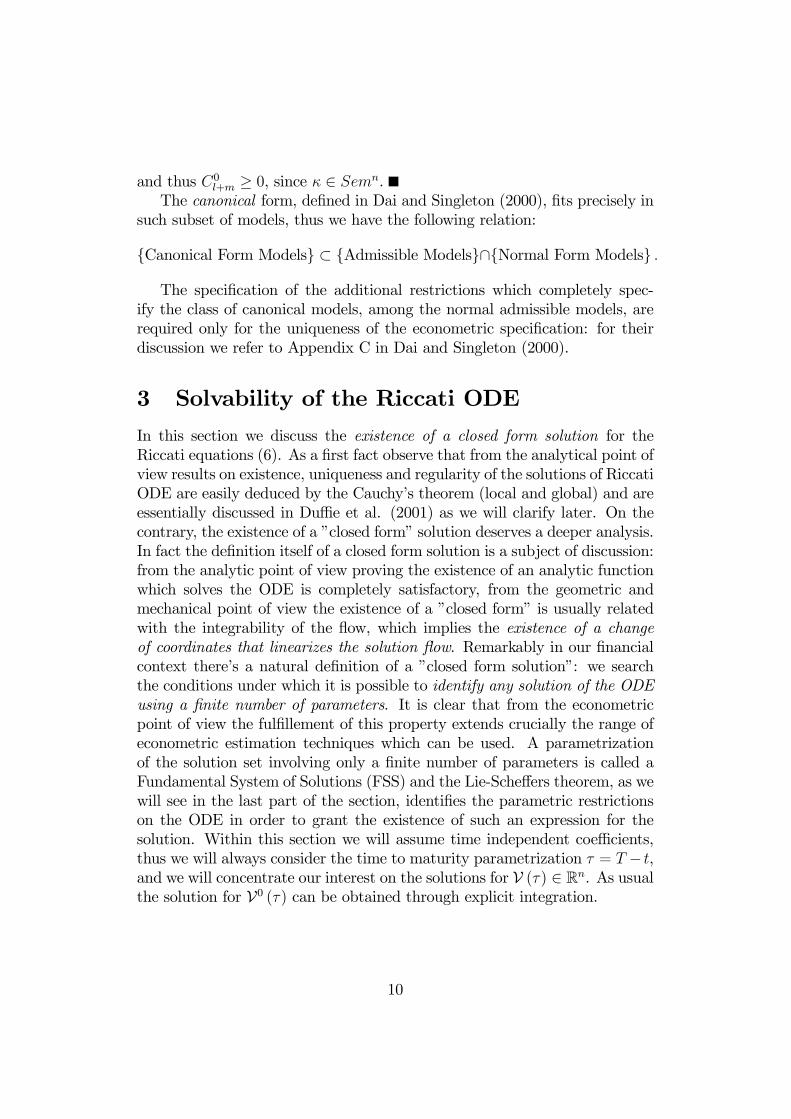
and thus C0l+m ≥ 0, since κ ∈ Semn.

The canonical form, defined in Dai and Singleton (2000), fits precisely insuch subset of models, thus we have the following relation:

Canonical Form Models ⊂ Admissible Models∩Normal Form Models .

The specification of the additional restrictions which completely spec-ify the class of canonical models, among the normal admissible models, arerequired only for the uniqueness of the econometric specification: for theirdiscussion we refer to Appendix C in Dai and Singleton (2000).

3 Solvability of the Riccati ODE

In this section we discuss the existence of a closed form solution for theRiccati equations (6). As a first fact observe that from the analytical point ofview results on existence, uniqueness and regularity of the solutions of RiccatiODE are easily deduced by the Cauchy’s theorem (local and global) and areessentially discussed in Duffie et al. (2001) as we will clarify later. On thecontrary, the existence of a ”closed form” solution deserves a deeper analysis.In fact the definition itself of a closed form solution is a subject of discussion:from the analytic point of view proving the existence of an analytic functionwhich solves the ODE is completely satisfactory, from the geometric andmechanical point of view the existence of a ”closed form” is usually relatedwith the integrability of the flow, which implies the existence of a changeof coordinates that linearizes the solution flow. Remarkably in our financialcontext there’s a natural definition of a ”closed form solution”: we searchthe conditions under which it is possible to identify any solution of the ODEusing a finite number of parameters. It is clear that from the econometricpoint of view the fulfillement of this property extends crucially the range ofeconometric estimation techniques which can be used. A parametrizationof the solution set involving only a finite number of parameters is called aFundamental System of Solutions (FSS) and the Lie-Scheffers theorem, as wewill see in the last part of the section, identifies the parametric restrictionson the ODE in order to grant the existence of such an expression for thesolution. Within this section we will assume time independent coefficients,thus we will always consider the time to maturity parametrization τ = T − t,and we will concentrate our interest on the solutions for V (τ) ∈ Rn. As usualthe solution for V0 (τ) can be obtained through explicit integration.

10

3.1 Series Expansion Solution

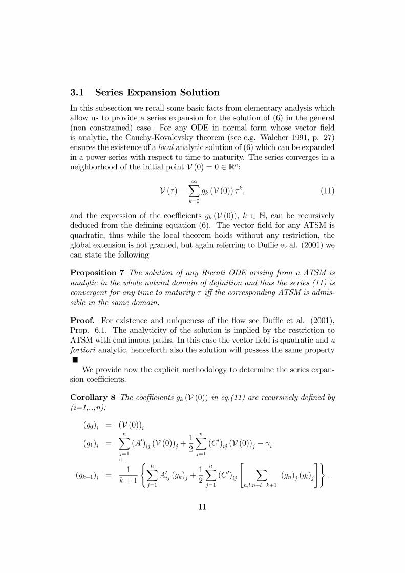
In this subsection we recall some basic facts from elementary analysis whichallow us to provide a series expansion for the solution of (6) in the general(non constrained) case. For any ODE in normal form whose vector fieldis analytic, the Cauchy-Kovalevsky theorem (see e.g. Walcher 1991, p. 27)ensures the existence of a local analytic solution of (6) which can be expandedin a power series with respect to time to maturity. The series converges in aneighborhood of the initial point V (0) = 0 ∈ Rn:

V (τ) =∞Xk=0

gk (V (0)) τk, (11)

and the expression of the coefficients gk (V (0)), k ∈ N, can be recursivelydeduced from the defining equation (6). The vector field for any ATSM isquadratic, thus while the local theorem holds without any restriction, theglobal extension is not granted, but again referring to Duffie et al. (2001) wecan state the following

Proposition 7 The solution of any Riccati ODE arising from a ATSM isanalytic in the whole natural domain of definition and thus the series (11) isconvergent for any time to maturity τ iff the corresponding ATSM is admis-sible in the same domain.

Proof. For existence and uniqueness of the flow see Duffie et al. (2001),Prop. 6.1. The analyticity of the solution is implied by the restriction toATSM with continuous paths. In this case the vector field is quadratic and afortiori analytic, henceforth also the solution will possess the same property

We provide now the explicit methodology to determine the series expan-sion coefficients.

Corollary 8 The coefficients gk (V (0)) in eq.(11) are recursively defined by(i=1,..,n):

(g0)i = (V (0))i(g1)i =

nXj=1

(A0)ij (V (0))j +1

2

nXj=1

(C 0)ij (V (0))j − γi

...

(gk+1)i =1

k + 1

(nX

j=1

A0ij (gk)j +1

2

nXj=1

(C 0)ij

" Xn,l:n+l=k+1

(gn)j (gl)j

#).

11

Proof. The expression for the coefficients is obtained computing the iteratedderivatives of the ODE expression (6).Numerical computation of the series expansion coefficients is one among

the possible approaches to determine the solution for a generic admissibleATSM. From our numerical checks it appears that the computation of atruncated series is by far the most efficient numerical method. It overper-forms numerical integration using the Runge-Kutta finite difference approachand the truncation error of the polynomial approximation becomes irrelevantfor any reasonable maturity with a mild number of coefficients. The trunca-tion error can be easily determined using the residual estimate for analyticfunctions.

3.2 Existence of a Fundamental System of Solutions

As we discussed in the previous section, the admissibility condition providesstrong parametric restrictions on the possible ATSM. The problem now is toaddress the following important question: under which parametric restric-tions can the model be solved in closed form?As a first step we observe that, due to the admissibility conditions, the

last m− n equations are linear and can be solved independently of the firstm nonlinear equations. Once their solution is given, the system of the firstm equations becomes a non homogeneous quadratic system.Before proceeding in the investigation of the non linear quadratic equa-

tions we must formalize the notion of Fundamental System of Solutions (FSS)which is due to Lie (see e.g. Walcher 1986):

Definition 9 An ODE is said to possess a Fundamental System of Solutions(FSS) if it is possible to express the solution as an analytic function Φ of afinite number d of special solutions V1 (τ) , ...,Vd (τ) and as a finite numberr of parameters k1 (V (0)) , ..., kr (V (0)) depending on the initial conditions:

V (V (0) , τ) = Φ¡V1 (τ) , ...,Vd (τ) , k1 (V (0)) , ..., kr (V (0))¢

The econometric follow up of the above definition is clear: such propertyallows for a fully parametric identification of the solution in terms of a finitenumber of parameters. We give now some examples in order to clarify theconcept of FSS.

Example 10 (Linear ODE) Any linear (possibly non homogeneous) ordi-nary differential equation admits a FSS. Consider for example the ODE (6)associated to a constant volatility n dimensional model (C = 0): in this case

12

the function Φ turns out to be affine, and any solution can be written in theform

ΦAff¡VP (τ) ,V1 (τ) , ...,Vn (τ) , k1 (V (0)) , ..., kn (V (0))¢

= VP (τ) +nXi=1

ki (V (0)) ¡V i (τ)− VP (τ)¢

where VP (τ) is a particular solution to the non homogeneous equation, whilethe differences V i (τ)− VP (τ), i = 1, .., n are solutions of the correspondinghomogeneous equation.

Example 11 (One dimensional Riccati) The simplest non linear exampleof ODE admitting a FSS is the one dimensional Riccati equation. Con-sider for example the ODE (6) when n = 1 and C 6= 0. It is possi-ble to verify (a more constructive proof will be provided in Appendix A)that any solution to this equation can be obtained in terms of three partic-ular solutions, VP1 (τ) ,VP2 (τ) ,VP3 (τ), corresponding to initial conditionsVP1 (0) ,VP2 (0) ,VP3 (0). In fact, for any generic solution V (τ) with initialcondition V (0), the following FSS can be found:

V (τ) = ΦCIR¡VP1 (τ) , ...,VP3 (τ) , k (V (0))¢ (12)

= VP2 (τ) +

·k (V (0)) V

P3 (τ)− VP1 (τ)

VP3 (τ)− VP2 (τ)− 1¸−1 ¡VP2 (τ)− VP1 (τ)

¢It is interesting to understand the geometric and algebraic origin of these

FSS; this can be done within the Lie group theory. Vector fields defining ODEare considered as elements of the Lie algebra which is defined as follows:

Definition 12 Let V be a finite dimensional real or complex vector spaceand U ⊂ V open and nonempty. By A (U,V) we denote the vector space ofall analytic maps from U into V. With the bracket defined by

[f (V) , g (V)] = ∇g (V) f (V)−∇f (V) g (V) , V ∈V,

for f, g ∈ A (U,V) we have that (A (V,V) , [, ]) is a Lie algebra.

Remarkably the Lie-Scheffers theorem provides a direct verification testin order to deduce whether an ODE possesses a FSS in terms of the vectorfields generating the ODE.

13

Theorem 13 (Lie Scheffers theorem, see e.g. Walcher 1991) The ODEddτV = F (V, τ) admits a Fundamental System of Solutions if and only if there

exist f1, .., fr ∈ A (V,V) and continuous parameters α1, ..., αr : R ⊃I → R,with r < +∞, such that

F (V, τ) =rX

i=1

αi (τ) fi (V) (13)

lie within a finite dimensional subalgebra L ⊂ A (V,V).

Example 14 (Linear ODE continued) Consider first a linear non homoge-neous ordinary differential equation of order n:

d

dτV = AV − γ, A ∈Mn.

Put γ = 0, then the corresponding finite dimensional Lie subalgebra of linearvector fields is isomorphic to Mn, [, ]c, the Lie Algebra of square matricesMn equipped with the commutator brackets

[A,B]c = AB −BA, A,B ∈Mn.

The matrix exponential map at time τ :

exp : Mn ×R+ → GLn

(A, τ) 7−→ exp (τA)

maps any linear vector field AV to the FSS of the corresponding ODE:

V (τ) = ΦLin (exp (τA) e1, ..., exp (τA) en,V1 (0) , ...,Vn (0))

=nXi=1

exp (τA) eiVi (0)

where ei are the elements of the canonical basis.The non homogeneous case (γ 6= 0) is a trivial extension: given a particu-

lar solution VP (τ), for any other solution V (τ), the difference V (τ)−VP (τ)solves the related homogeneous equation, thus:

V (τ) = VP (τ) + ΦLin¡V1 (τ)− VP (τ) , ...,Vn (τ)− VP (τ) , k1 (V (0)) , ..., kn (V (0))

¢= ΦAff

¡VP (τ) ,V1 (τ) , ...,Vn (τ) , k1 (V (0)) , ..., kn (V (0))¢

14

The previous example plays a crucial role, in fact it can be shown thatevery finite dimensional Lie Algebra is isomorphic to the Lie subalgebra ofthe general linear group GLn for a finite dimensional vector space V , wheren = dimV (see e.g. Duistermaat and Kolk 1999 pg.88). As a consequence,the Lie-Scheffers theorem provides a constructive and powerful scheme inorder to produce FSS and to linearize the flow of the ODE: in other words,the existence of a finite dimensional Lie subalgebra implies the existence ofan isomorphic system of coordinates under which the ODE become linear.This system is the one which realizes the Lie algebra of vector fields as a Liesubalgebra of matrices GLn (linear representation).

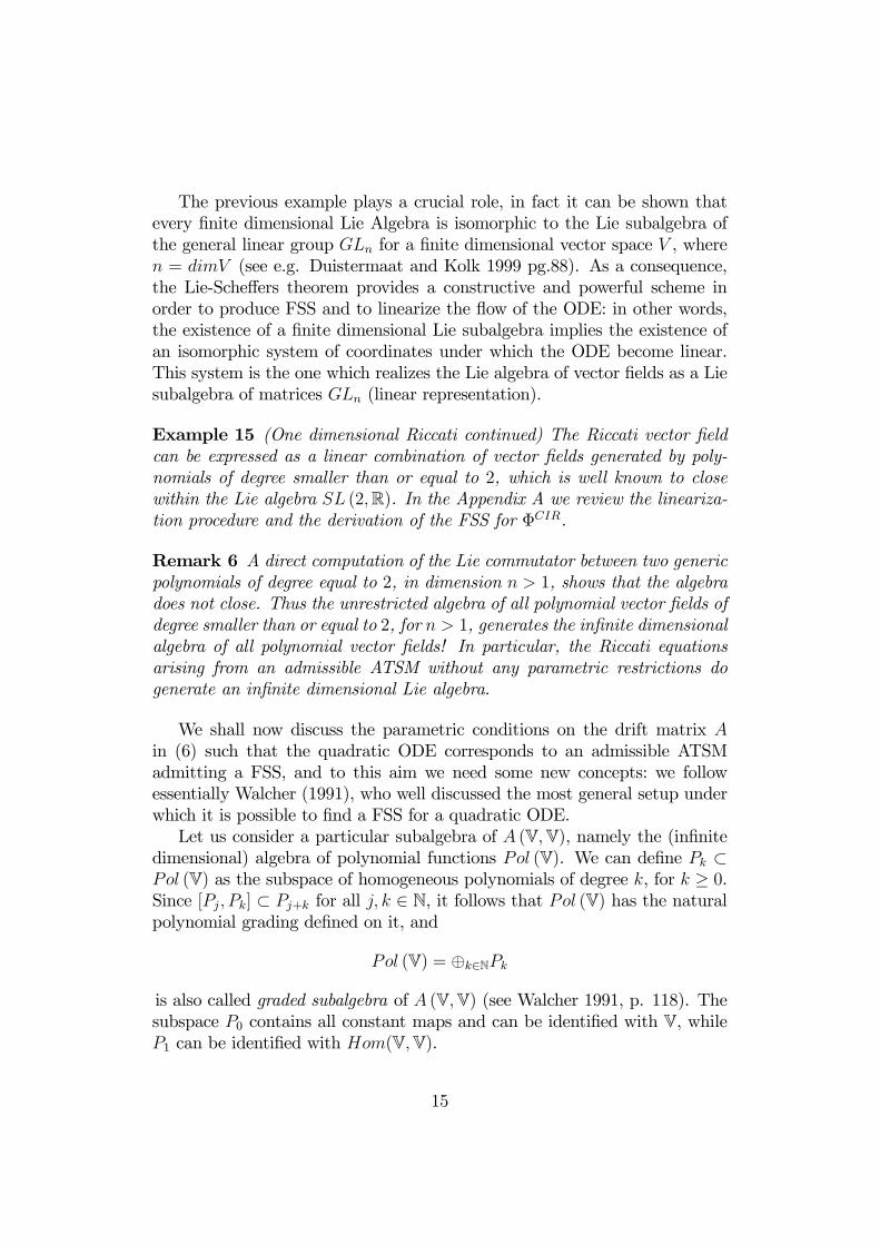
Example 15 (One dimensional Riccati continued) The Riccati vector fieldcan be expressed as a linear combination of vector fields generated by poly-nomials of degree smaller than or equal to 2, which is well known to closewithin the Lie algebra SL (2,R). In the Appendix A we review the lineariza-tion procedure and the derivation of the FSS for ΦCIR.

Remark 6 A direct computation of the Lie commutator between two genericpolynomials of degree equal to 2, in dimension n > 1, shows that the algebradoes not close. Thus the unrestricted algebra of all polynomial vector fields ofdegree smaller than or equal to 2, for n > 1, generates the infinite dimensionalalgebra of all polynomial vector fields! In particular, the Riccati equationsarising from an admissible ATSM without any parametric restrictions dogenerate an infinite dimensional Lie algebra.

We shall now discuss the parametric conditions on the drift matrix Ain (6) such that the quadratic ODE corresponds to an admissible ATSMadmitting a FSS, and to this aim we need some new concepts: we followessentially Walcher (1991), who well discussed the most general setup underwhich it is possible to find a FSS for a quadratic ODE.Let us consider a particular subalgebra of A (V,V), namely the (infinite

dimensional) algebra of polynomial functions Pol (V). We can define Pk ⊂Pol (V) as the subspace of homogeneous polynomials of degree k, for k ≥ 0.Since [Pj, Pk] ⊂ Pj+k for all j, k ∈ N, it follows that Pol (V) has the naturalpolynomial grading defined on it, and

Pol (V) = ⊕k∈NPk

is also called graded subalgebra of A (V,V) (see Walcher 1991, p. 118). Thesubspace P0 contains all constant maps and can be identified with V, whileP1 can be identified with Hom(V,V).

15

Remark 7 It is easy to verify that P0 ⊕ P1 is always a closed subalgebraof Pol(V): this reflects the fact that linear differential equations admit afundamental system of solutions.

We are interested in finite dimensional subalgebras of A (V,V), and inparticular in graded subalgebras of the type

L = L0 ⊕ ...⊕ Lk,

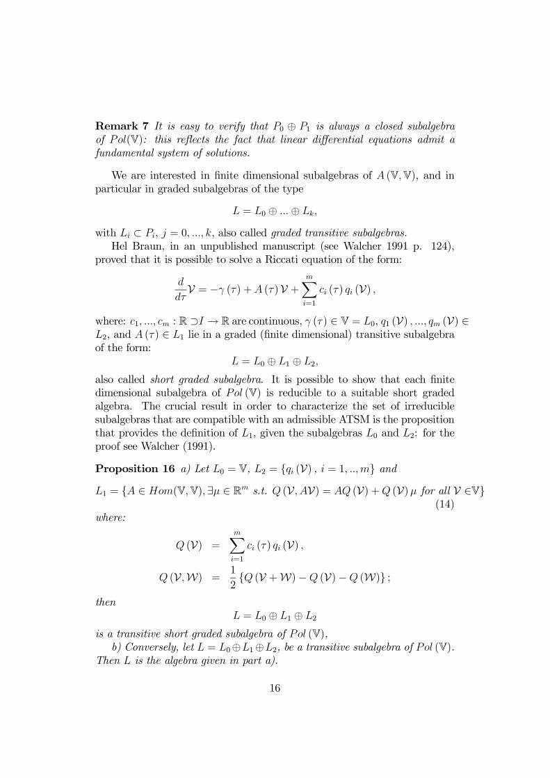
with Li ⊂ Pi, j = 0, ..., k, also called graded transitive subalgebras.Hel Braun, in an unpublished manuscript (see Walcher 1991 p. 124),

proved that it is possible to solve a Riccati equation of the form:

d

dτV = −γ (τ) +A (τ)V +

mXi=1

ci (τ) qi (V) ,

where: c1, ..., cm : R ⊃I → R are continuous, γ (τ) ∈ V = L0, q1 (V) , ..., qm (V) ∈L2, and A (τ) ∈ L1 lie in a graded (finite dimensional) transitive subalgebraof the form:

L = L0 ⊕ L1 ⊕ L2,

also called short graded subalgebra. It is possible to show that each finitedimensional subalgebra of Pol (V) is reducible to a suitable short gradedalgebra. The crucial result in order to characterize the set of irreduciblesubalgebras that are compatible with an admissible ATSM is the propositionthat provides the definition of L1, given the subalgebras L0 and L2: for theproof see Walcher (1991).

Proposition 16 a) Let L0 = V, L2 = qi (V) , i = 1, ..,m andL1 = A ∈ Hom(V,V),∃µ ∈ Rm s.t. Q (V, AV) = AQ (V) +Q (V)µ for all V ∈V

(14)where:

Q (V) =mXi=1

ci (τ) qi (V) ,

Q (V,W) =1

2Q (V +W)−Q (V)−Q (W) ;

thenL = L0 ⊕ L1 ⊕ L2

is a transitive short graded subalgebra of Pol (V),b) Conversely, let L = L0⊕L1⊕L2, be a transitive subalgebra of Pol (V).

Then L is the algebra given in part a).

16

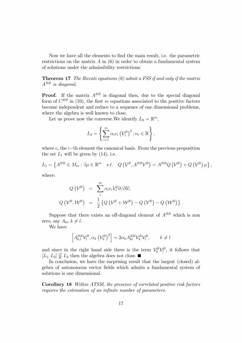
Now we have all the elements to find the main result, i.e. the parametricrestrictions on the matrix A in (6) in order to obtain a fundamental systemof solutions under the admissibility restrictions:

Theorem 17 The Riccati equations (6) admit a FSS if and only if the matrixABB is diagonal.

Proof. If the matrix ABB is diagonal then, due to the special diagonalform of CBB in (10), the first m equations associated to the positive factorsbecome independent and reduce to a sequence of one dimensional problems,where the algebra is well known to close.Let us prove now the converse.We identify L0 = Rm,

L2 =

(mXi=1

αiei¡VB

i

¢2;αi ∈ R

),

where ei the i−th element the canonical basis. From the previous propositionthe set L1 will be given by (14), i.e.

L1 =©ABB ∈Mm : ∃µ ∈ Rm s.t. Q

¡VB, ABBVB¢= ABBQ

¡VB¢+Q

¡VB¢µª,

where:

Q¡VB

¢=

mXi

αieiV2i ∂/∂Vi

Q¡VB,WB

¢=

1

2

©Q¡VB +WB

¢−Q¡VB

¢−Q¡WB

¢ª.

Suppose that there exists an off-diagonal element of ABB which is nonzero, say Akl, k 6= l.We have h

ABBk,l VB

l , αk

¡VBk

¢2i= 2αkA

BBkl VB

k VBl , k 6= l

and since in the right hand side there is the term VBk VB

l , it follows that[L1, L2] " L2 then the algebra does not close.In conclusion, we have the surprising result that the largest (closed) al-

gebra of autonomous vector fields which admits a fundamental system ofsolutions is one dimensional.

Corollary 18 Within ATSM, the presence of correlated positive risk factorsrequires the estimation of an infinite number of parameters.

17

Remark 8 Our results have been derived under very restrictive assumptions(affine definition of factors and short rate, time-homogeneous Markov set-ting, admissibility conditions and market completeness). However, the abovealgebraic arguments can be applied in full generality to discuss the existenceof a FSS for the Riccati equations arising from any finite dimensional re-alization of the Heath, Jarrow and Morton (1992) model (see Filipovic andTeichmann 2003). This extension requires a classification of the short gradedtransitive subalgebras of Pol (V).

3.3 Separable Polinomial Term Structure Models ad-mitting a FSS

The conditions for the existence of a FSS can be extended without essentialincrease of complexity to any consistent (see Björk 2003) polynomial termstructure model, thanks to the results of Filipovic (2002).

Definition 19 A polynomial term structure model is defined by:

- the factors Zt defined in a cone domain Z ⊆Rn, whose dynamics under therisk neutral measure Q satisfy the following SDE:

dZt = b (Zt) dt+ σ (Zt) dWt Zt ∈ Z,

where Wt is a n-dimensional Brownian motion, and the drift b (.) andvolatility σ (.) satisfy the growth constraint:

kb (z)k+ kσ (z)k ≤ C (1 + kzk) , ∀z ∈ Z

- the forward rate curve:

r (Zt, τ) =dX

|i|=0gi (τ) (Zt)

i , τ ≥ 0, (15)

where the multindex notation has been used: i = (i1, ..., im), |i| = i1 +... + im and zi = zi11 ...z

inn ; here d denotes the degree of the polynomial

term structure.

The cases d = 1 (ATSM with Zt = Yt) and d = 2 (quadratic termstructure models) are the only relevant polynomial term structure models,as proved in the following theorem due to Filipovic (2002):

18

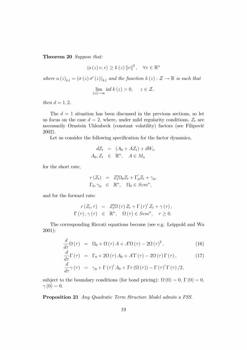
Theorem 20 Suppose that:

ha (z) v, vi ≥ k (z) kvk2 , ∀v ∈ Rn

where a (z)k,l = (σ (z)σ0 (z))k,l and the function k (z) : Z → R is such that

limkzk→∞

inf k (z) > 0, z ∈ Z,

then d = 1, 2.

The d = 1 situation has been discussed in the previous sections, so letus focus on the case d = 2, where, under mild regularity conditions, Zt arenecessarily Ornstein Uhlenbeck (constant volatility) factors (see Filipovic2002).Let us consider the following specification for the factor dynamics,

dZt = (A0 +AZt) + dWt,

A0, Zt ∈ Rn, A ∈Mn

for the short rate,

r (Zt) = Z 0tΩ0Zt + Γ00Zt + γ0,

Γ0, γ0 ∈ Rn, Ω0 ∈ Semn,

and for the forward rate:

r (Zt, τ) = Z 0tΩ (τ)Zt + Γ (τ)0 Zt + γ (τ) ,

Γ (τ) , γ (τ) ∈ Rn, Ω (τ) ∈ Semn, τ ≥ 0.The corresponding Riccati equations become (see e.g. Leippold and Wu

2001):

d

dτΩ (τ) = Ω0 + Ω (τ)A+A0Ω (τ)− 2Ω (τ)2 , (16)

d

dτΓ (τ) = Γ0 + 2Ω (τ)A0 +A0Γ (τ)− 2Ω (τ)Γ (τ) , (17)

d

dτγ (τ) = γ0 + Γ (τ)0A0 + Tr (Ω (τ))− Γ (τ)0 Γ (τ) /2,

subject to the boundary conditions (for bond pricing): Ω (0) = 0, Γ (0) = 0,γ (0) = 0.

Proposition 21 Any Quadratic Term Structure Model admits a FSS.

19

Proof. The Matrix Riccati Equation can be written as a linear combinationof generators of the closed short graded algebra sl (2n) with its natural grad-ing (see Lafortune and Winternitz 1996). Hence, due to the Lie-Schefferstheorem, it admits a FSS.

Remark 9 Notice that the non linear equation for Ω (τ) is a standard MatrixSymmetric Riccati Equation (for a survey see e.g. Reid 1972 or Freiling2002), and it is well known that its flow corresponds to a linear flow ona Lagrangian Grassmanian manifold (the multi dimensional generalizationof projective spaces), hence in this case the linear flow can be found by astandard homogeneization procedure (see at end of this section for the explicitconstruction of the linear flow).

Given the solution for Ω (τ), the equation for Γ (τ) and for γ (τ) can besolved by simple integration.We can thus completely classify the Polynomial Term Structure Models

whose non linear equations admit a Fundamental System of Solutions. Inthe following subsection we provide the closed form expression for (6) for all(separable) term structure models admitting a FSS.

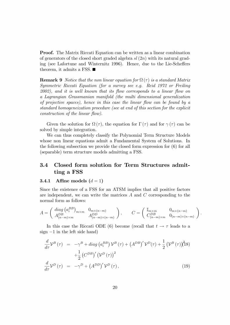
3.4 Closed form solution for Term Structures admit-ting a FSS

3.4.1 Affine models (d = 1)

Since the existence of a FSS for an ATSM implies that all positive factorsare independent, we can write the matrices A and C corresponding to thenormal form as follows:

A =

µdiag

¡aBBi

¢m×m 0m×(n−m)

ADB(n−m)×m ADD

(n−m)×(n−m)

¶, C =

µIm×m 0m×(n−m)CDB(n−m)×m 0(n−m)×(n−m)

¶.

In this case the Riccati ODE (6) become (recall that t → τ leads to asign −1 in the left side hand)

d

dτVB (τ) = −γB + diag

¡aBBi

¢VB (τ) +¡ADB

¢0 VD(τ) +1

2

¡VB (τ)¢2(18)

+1

2

¡CDB

¢0 ¡VD (τ)¢2

d

dτVD (τ) = −γD + ¡ADD

¢0 VD (τ) , (19)

20

where

VB = (V1, .....,Vm)0 ,¡VB¢2

=¡V21 , .....,V2m¢0 ,

VD = (Vm+1, .....,Vn)0 ,¡VD¢2

=¡V2m+1, .....,V2n¢0 ,

γB = (γ1, ....., γm)0 ,

γD =¡γm+1, ....., γn

¢0,

with boundary condition V(0) = u.In analogy with Duffie et al. (2001), we assume in (6) that γi ≥ 0,

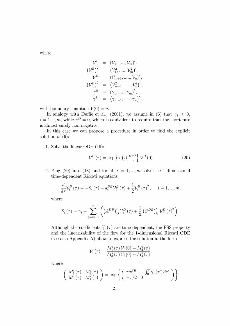
i = 1, ..,m, while γD = 0, which is equivalent to require that the short rateis almost surely non negative.In this case we can propose a procedure in order to find the explicit

solution of (6):

1. Solve the linear ODE (19):

VD (τ) = expnτ¡ADD

¢0oVD (0) (20)

2. Plug (20) into (18) and for all i = 1, ...,m solve the 1-dimensionaltime-dependent Riccati equations

d

dτVBi (τ) = −eγi (τ) + aBBi VB

i (τ) +1

2VBi (τ)

2 , i = 1, ...,m,

where

eγi (τ) = γi −nX

j=m+1

µ¡ADB

¢0ijVDj (τ) +

1

2

¡CDB

¢0ijVDj (τ)

2

¶.

Although the coefficients eγi (τ) are time dependent, the FSS propertyand the linearizability of the flow for the 1-dimensional Riccati ODE(see also Appendix A) allow to express the solution in the form

Vi (τ) = M i1 (τ)Vi (0) +M i

2 (τ)

M i3 (τ)Vi (0) +M i

4 (τ),

whereµM i1 (τ) M i

2 (τ)M i3 (τ) M i

4 (τ)

¶= exp

½µτaBB1 − R τ

0eγi (τ 0) dτ 0

−τ/2 0

¶¾21

and the integral Z τ

0

eγi (τ 0) dτ 0can be explicitly performed, since the general expression of

R τ0eγi (τ 0) dτ 0

will be an affine combination of exponentials and the expressions forthe M i

j , j = 1, ..., 4 are obtained through exponentiation of an explicitexpression.

Remark 10 The assumption γD = 0 is not restrictive, since alternatively wecan search for a stationary time independent solution V∗ solving the algebraicsystem dV∗ (τ) /dτ = 0: then for any solution V of the original equation thedifference V − V∗ solves the corresponding homogeneous equation.

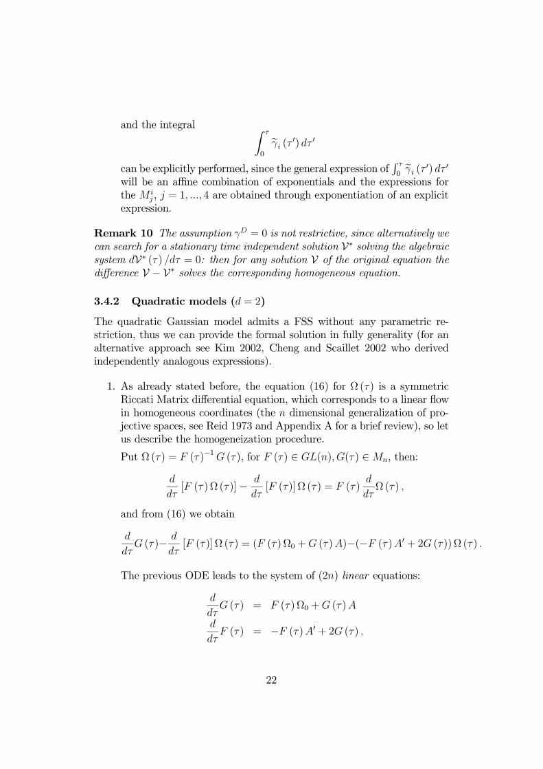
3.4.2 Quadratic models (d = 2)

The quadratic Gaussian model admits a FSS without any parametric re-striction, thus we can provide the formal solution in fully generality (for analternative approach see Kim 2002, Cheng and Scaillet 2002 who derivedindependently analogous expressions).

1. As already stated before, the equation (16) for Ω (τ) is a symmetricRiccati Matrix differential equation, which corresponds to a linear flowin homogeneous coordinates (the n dimensional generalization of pro-jective spaces, see Reid 1973 and Appendix A for a brief review), so letus describe the homogeneization procedure.

Put Ω (τ) = F (τ)−1G (τ), for F (τ) ∈ GL(n), G(τ) ∈Mn, then:

d

dτ[F (τ)Ω (τ)]− d

dτ[F (τ)]Ω (τ) = F (τ)

d

dτΩ (τ) ,

and from (16) we obtain

d

dτG (τ)− d

dτ[F (τ)]Ω (τ) = (F (τ)Ω0 +G (τ)A)−(−F (τ)A0 + 2G (τ))Ω (τ) .

The previous ODE leads to the system of (2n) linear equations:

d

dτG (τ) = F (τ)Ω0 +G (τ)A

d

dτF (τ) = −F (τ)A0 + 2G (τ) ,

22

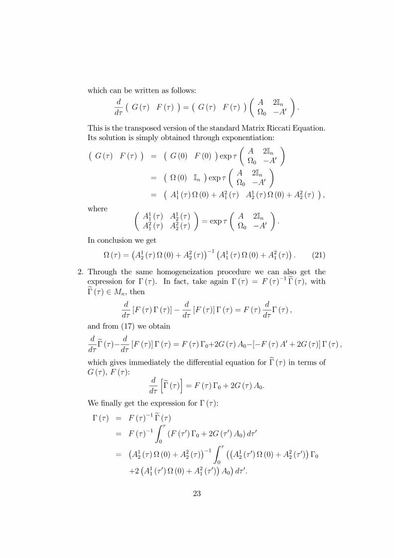
which can be written as follows:d

dτ

¡G (τ) F (τ)

¢=¡G (τ) F (τ)

¢µ A 2InΩ0 −A0

¶.

This is the transposed version of the standard Matrix Riccati Equation.Its solution is simply obtained through exponentiation:¡G (τ) F (τ)

¢=

¡G (0) F (0)

¢exp τ

µA 2InΩ0 −A0

¶=

¡Ω (0) In

¢exp τ

µA 2InΩ0 −A0

¶=

¡A11 (τ)Ω (0) +A21 (τ) A12 (τ)Ω (0) +A22 (τ)

¢,

where µA11 (τ) A12 (τ)A21 (τ) A22 (τ)

¶= exp τ

µA 2InΩ0 −A0

¶.

In conclusion we get

Ω (τ) =¡A12 (τ)Ω (0) +A22 (τ)

¢−1 ¡A11 (τ)Ω (0) +A21 (τ)

¢. (21)

2. Through the same homogeneization procedure we can also get theexpression for Γ (τ). In fact, take again Γ (τ) = F (τ)−1 eΓ (τ), witheΓ (τ) ∈Mn, then

d

dτ[F (τ)Γ (τ)]− d

dτ[F (τ)]Γ (τ) = F (τ)

d

dτΓ (τ) ,

and from (17) we obtain

d

dτeΓ (τ)− d

dτ[F (τ)]Γ (τ) = F (τ)Γ0+2G (τ)A0−[−F (τ)A0 + 2G (τ)]Γ (τ) ,

which gives immediately the differential equation for eΓ (τ) in terms ofG (τ), F (τ):

d

dτ

heΓ (τ)i = F (τ)Γ0 + 2G (τ)A0.

We finally get the expression for Γ (τ):

Γ (τ) = F (τ)−1 eΓ (τ)= F (τ)−1

Z τ

0

(F (τ 0)Γ0 + 2G (τ 0)A0) dτ 0

=¡A12 (τ)Ω (0) +A22 (τ)

¢−1 Z τ

0

¡¡A12 (τ

0)Ω (0) +A22 (τ0)¢Γ0

+2¡A11 (τ

0)Ω (0) +A21 (τ0)¢A0¢dτ 0.

23

3. As usual, γ (τ) can be obtained by direct integration.

References

[1] Björk, T. (2003): ”On the Geometry of Interest Rates Models”. Forth-coming in Springer Lecture Notes in Mathematics.

[2] Brown, R. and S. Schaefer (1994): ”Interest rate volatility and the shapeof the term structure”. Philosophical Transactions of the Royal Society:Physical Sciences and Engineering, 347, 449-598.

[3] Cox, J. C., Ingersoll J. E. and . Ross, S. A (1985): ”A Theory of theTerm Structure of Interest Rates”. Econometrica, 53, 385-408.

[4] Carinena, J. F., Marmo G., and Nasarre, J. (1998): ”The non-linear su-perposition principle and the Wei-Norman method”. Int. J. Mod. Phys.A 13, 3601-27.

[5] Cheng, P. and O. Scaillet (2002): ”Linear-Quadratic Jump-DiffusionModelling with Application to Stochastic Volatility”. Preprint.

[6] Dai, Q. and K. Singleton (2000): ”Specification Analysis of Affine TermStructure Models”. Journal of Finance, 55, 1943-1978.

[7] Duffie, D., D. Filipovic and W. Schachermayer (2001): ”Affine Pro-cesses and Applications in Finance”, forthcoming in Annals of AppliedProbability.

[8] Duffie, D. and R. Kan (1996): ”A Yield-Factor Model of Interest Rates”.Mathematical Finance, 6 (4), 379-406.

[9] Duffie, D., J. Pan and K. Singleton (2000): Transform analysis and assetpricing for affine jump-diffusions”. Econometrica, 68, 1343-1376.

[10] Duistermaat, J.J. and J.A.C. Kolk (1999): ”Lie Groups”. Springer Ver-lag.

[11] Elliott, R. J. and J. van der Hoek (2001): ”Stochastic flows and theforward measure”. Finance and Stochastics, 5, 511-525.

[12] Filipovic, D. (2002): ”Separable term structures and the maximal degreeproblem”. Mathematical Finance, 12 (4), 341-349.

24

[13] Filipovic, D. and J. Teichmann (2003): ”Existence of invariant manifoldsfor stochastic equations in infinite dimension”. J. Functional Analysis,197, 398-432.

[14] Freiling, G. (2002): ”A Survey of Nonsymmetric Riccati Equations”.Linear Algebra and Its Applications, 243-270.

[15] Heath, D., R. Jarrow and A. Morton (1992): ”Bond pricing and the termstructure of interest rates: A new methodology for contingent claimsvaluation. Econometrica, 60, 77-105.

[16] Grasselli, M. and C. Tebaldi (2004): ”Impulse-Response analysis andImmunization in Affine Term Structure Models”. Preprint.

[17] Kim, D. H. (2003): ”Time-varing risk and return in the Quadratic-Gaussian Model of the term structure”. Preprint.

[18] Lafortune, S. and P. Winternitz (1996): ”Superposition formulas forpseudounitary Riccati equations”. J. Math. Phys., 37, 1539-1550.

[19] Leippold, M. and L. Wu (2001): ”Design and Estimation of QuadraticTerm Structure Models”. Working Paper. University of Zurich and Ford-ham University.

[20] Reid, W. T. (1972): ”Riccati differential equations”. Academic Press:New York.

[21] Walcher, S. (1991): ”Algebras and Differential Equations”. HadronicPress.

[22] Walcher, S. (1986): ” Uber polynomiale, insbesondere Riccatische, Dif-ferentialgleichungen mit Fundamentallosungen”. Math. Ann. 275, 269-280.

4 Appendix A

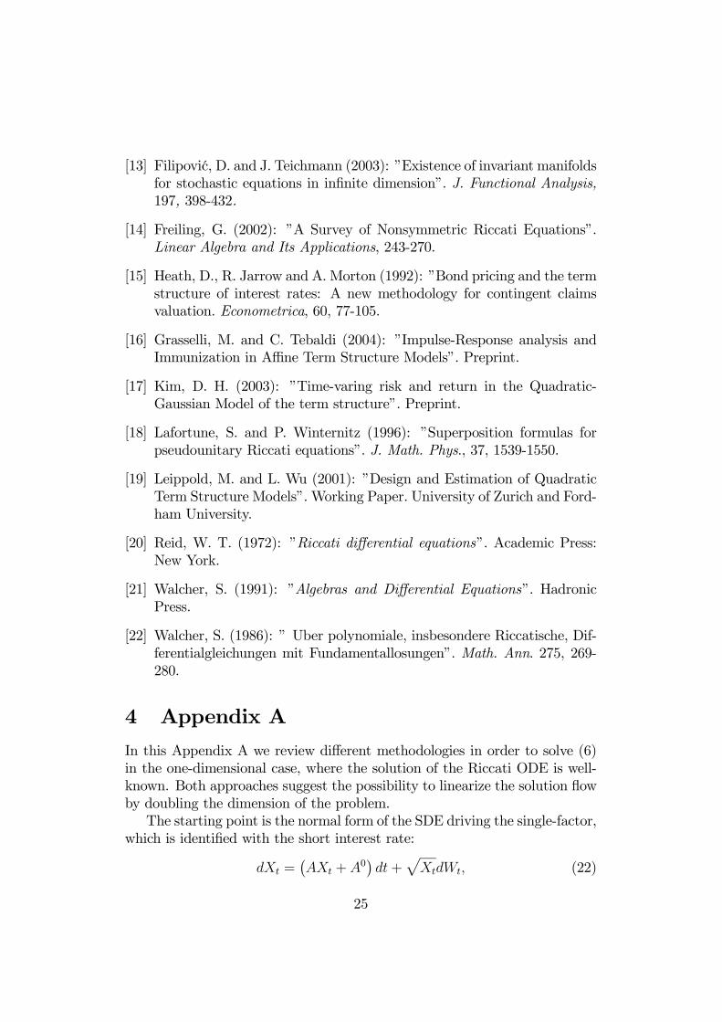
In this Appendix A we review different methodologies in order to solve (6)in the one-dimensional case, where the solution of the Riccati ODE is well-known. Both approaches suggest the possibility to linearize the solution flowby doubling the dimension of the problem.The starting point is the normal form of the SDE driving the single-factor,

which is identified with the short interest rate:

dXt =¡AXt +A0

¢dt+

pXtdWt, (22)

25

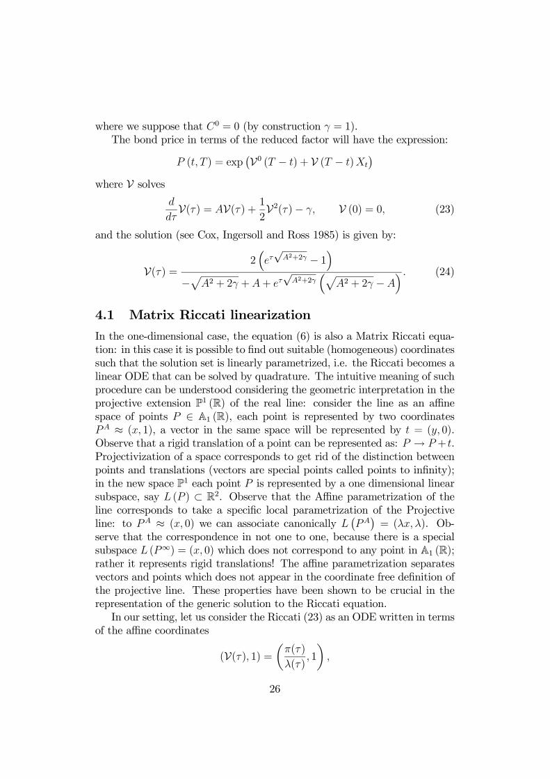
where we suppose that C0 = 0 (by construction γ = 1).The bond price in terms of the reduced factor will have the expression:

P (t, T ) = exp¡V0 (T − t) + V (T − t)Xt

¢where V solves

d

dτV(τ) = AV(τ) + 1

2V2(τ)− γ, V (0) = 0, (23)

and the solution (see Cox, Ingersoll and Ross 1985) is given by:

V(τ) =2³eτ√

A2+2γ − 1´

−pA2 + 2γ +A+ eτ√

A2+2γ³p

A2 + 2γ −A´ . (24)

4.1 Matrix Riccati linearization

In the one-dimensional case, the equation (6) is also a Matrix Riccati equa-tion: in this case it is possible to find out suitable (homogeneous) coordinatessuch that the solution set is linearly parametrized, i.e. the Riccati becomes alinear ODE that can be solved by quadrature. The intuitive meaning of suchprocedure can be understood considering the geometric interpretation in theprojective extension P1 (R) of the real line: consider the line as an affinespace of points P ∈ A1 (R), each point is represented by two coordinatesPA ≈ (x, 1), a vector in the same space will be represented by t = (y, 0).Observe that a rigid translation of a point can be represented as: P → P + t.Projectivization of a space corresponds to get rid of the distinction betweenpoints and translations (vectors are special points called points to infinity);in the new space P1 each point P is represented by a one dimensional linearsubspace, say L (P ) ⊂ R2. Observe that the Affine parametrization of theline corresponds to take a specific local parametrization of the Projectiveline: to PA ≈ (x, 0) we can associate canonically L

¡PA¢= (λx, λ). Ob-

serve that the correspondence in not one to one, because there is a specialsubspace L (P∞) = (x, 0) which does not correspond to any point in A1 (R);rather it represents rigid translations! The affine parametrization separatesvectors and points which does not appear in the coordinate free definition ofthe projective line. These properties have been shown to be crucial in therepresentation of the generic solution to the Riccati equation.In our setting, let us consider the Riccati (23) as an ODE written in terms

of the affine coordinates

(V(τ), 1) =µπ(τ)

λ(τ), 1

¶,

26

such thatd

dτV(τ) = − π(τ)

λ2(τ)

d

dτλ(τ) +

1

λ(τ)

d

dτπ(τ).

If we rewrite the equation in terms of the homogeneous coordinates (π(τ), λ(τ)),it becomes:

λ(τ)d

dτπ(τ)− π(τ)

d

dτλ(τ) = (−γλ(τ) +Aπ(τ))λ(τ) +

µ1

2π(τ)

¶π(τ),

which can be written as a linear ODE:

d

dτ

µπ(τ)λ(τ)

¶=

µA −γ−120

¶µπ(τ)λ(τ)

¶,

whose solution is given byµπ(τ)λ(τ)

¶= exp

½τ

µA −γ−120

¶¾µπ0λ0

¶.

If we denoteµa1(τ) a2(τ)a3(τ) a4(τ)

¶= exp

½τ

µA −γ−120

¶¾, (25)

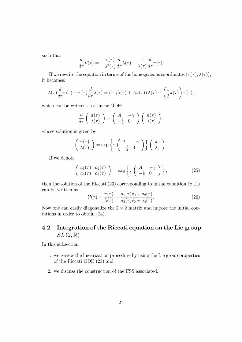
then the solution of the Riccati (23) corresponding to initial condition (v0, 1)can be written as

V(τ) = π(τ)

λ(τ)=

a1(τ)v0 + a2(τ)

a3(τ)v0 + a4(τ). (26)

Now one can easily diagonalize the 2× 2 matrix and impose the initial con-ditions in order to obtain (24).

4.2 Integration of the Riccati equation on the Lie groupSL (2,R)

In this subsection

1. we review the linearization procedure by using the Lie group propertiesof the Riccati ODE (23) and

2. we discuss the construction of the FSS associated.

27

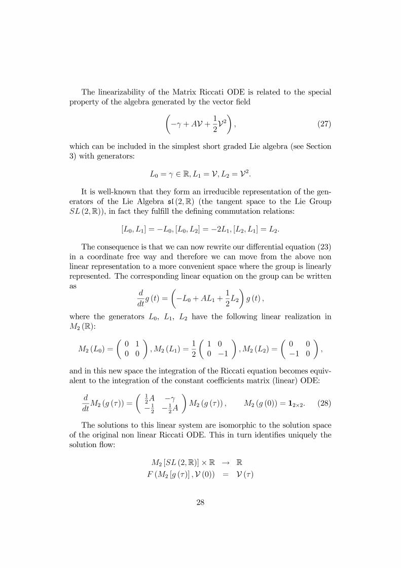
The linearizability of the Matrix Riccati ODE is related to the specialproperty of the algebra generated by the vector fieldµ

−γ +AV + 12V2¶, (27)

which can be included in the simplest short graded Lie algebra (see Section3) with generators:

L0 = γ ∈ R, L1 = V, L2 = V2.

It is well-known that they form an irreducible representation of the gen-erators of the Lie Algebra sl (2,R) (the tangent space to the Lie GroupSL (2,R)), in fact they fulfill the defining commutation relations:

[L0, L1] = −L0, [L0, L2] = −2L1, [L2, L1] = L2.

The consequence is that we can now rewrite our differential equation (23)in a coordinate free way and therefore we can move from the above nonlinear representation to a more convenient space where the group is linearlyrepresented. The corresponding linear equation on the group can be writtenas

d

dtg (t) =

µ−L0 +AL1 +

1

2L2

¶g (t) ,

where the generators L0, L1, L2 have the following linear realization inM2 (R):

M2 (L0) =

µ0 10 0

¶,M2 (L1) =

1

2

µ1 00 −1

¶,M2 (L2) =

µ0 0−1 0

¶,

and in this new space the integration of the Riccati equation becomes equiv-alent to the integration of the constant coefficients matrix (linear) ODE:

d

dtM2 (g (τ)) =

µ12A −γ−12−12A

¶M2 (g (τ)) , M2 (g (0)) = 12×2. (28)

The solutions to this linear system are isomorphic to the solution spaceof the original non linear Riccati ODE. This in turn identifies uniquely thesolution flow:

M2 [SL (2,R)]× R → RF (M2 [g (τ)] ,V (0)) = V (τ)

28

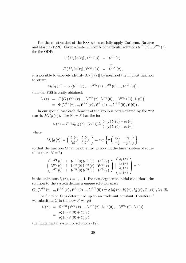
For the construction of the FSS we essentially apply Carinena, NasarreandMarmo (1999). Given a finite numberN of particular solutions VP1 (τ) ...VPN (τ)for the ODE:

F¡M2 [g (τ)] ,VP1 (0)

¢= VP1 (τ)

...

F¡M2 [g (τ)] ,VPN (0)

¢= VPN (τ) ,

it is possible to uniquely identifyM2 [g (τ)] by means of the implicit functiontheorem:

M2 [g (τ)] = G¡VP1 (τ) , ..,VPN (τ) ,VP1 (0) , ..,VPN (0)

¢,

thus the FSS is easily obtained:

V (τ) = F¡G¡VP1 (τ) , ..,VPN (τ) ,VP1 (0) , ..,VPN (0)

¢,V (0)¢

= Φ¡VP1 (τ) , ..,VPN (τ) ,VP1 (0) , ..,VPN (0) ,V (0)¢ .

In our special case each element of the group is parametrized by the 2x2matrix M2 (g (τ)). The Flow F has the form:

V (τ) = F (M2 [g (τ)] ,V (0)) , b1 (τ)V (0) + b2 (τ)

b3 (τ)V (0) + b4 (τ)

where:

M2 [g (τ)] =

µb1(τ) b2(τ)b3(τ) b4(τ)

¶= exp

½τ

µ12A −γ−12−12A

¶¾,

so that the function G can be obtained by solving the linear system of equa-tions (here N = 3) VP1 (0) 1 VP1 (0)VP1 (τ) VP1 (τ)

VP2 (0) 1 VP2 (0)VP2 (τ) VP2 (τ)VP3 (0) 1 VP3 (0)VP3 (τ) VP3 (τ)

b1 (τ)b2 (τ)b3 (τ)b4 (τ)

= 0

in the unknowns bi (τ), i = 1, .., 4. For non degenerate initial conditions, thesolution to the system defines a unique solution space

Gλ

¡VP1 (τ) , ..,VPN (τ) ,VP1 (0) , ..,VPN (0)¢, λ (bs1 (τ) , b

s2 (τ) , b

s3 (τ) , b

s4 (τ))

0 , λ ∈ R.The function G is determined up to an irrelevant constant, therefore if

we substitute G in the flow F we get:

V (τ) = ΦCIR¡VP1 (τ) , ..,VPN (τ) ,VP1 (0) , ..,VPN (0) ,V (0)¢

=bs1 (τ)V (0) + bs2 (τ)

bs3 (τ)V (0) + bs4 (τ),

the fundamental system of solutions (12).

29

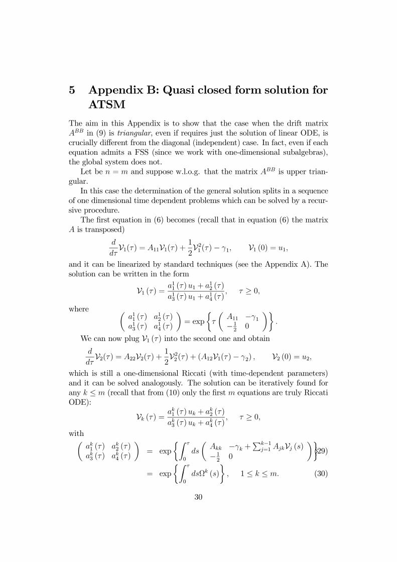
5 Appendix B: Quasi closed form solution forATSM

The aim in this Appendix is to show that the case when the drift matrixABB in (9) is triangular, even if requires just the solution of linear ODE, iscrucially different from the diagonal (independent) case. In fact, even if eachequation admits a FSS (since we work with one-dimensional subalgebras),the global system does not.Let be n = m and suppose w.l.o.g. that the matrix ABB is upper trian-

gular.In this case the determination of the general solution splits in a sequence

of one dimensional time dependent problems which can be solved by a recur-sive procedure.The first equation in (6) becomes (recall that in equation (6) the matrix

A is transposed)

d

dτV1(τ) = A11V1(τ) + 1

2V21 (τ)− γ1, V1 (0) = u1,

and it can be linearized by standard techniques (see the Appendix A). Thesolution can be written in the form

V1 (τ) = a11 (τ)u1 + a12 (τ)

a13 (τ)u1 + a14 (τ), τ ≥ 0,

where µa11 (τ) a12 (τ)a13 (τ) a14 (τ)

¶= exp

½τ

µA11 −γ1−120

¶¾.

We can now plug V1 (τ) into the second one and obtaind

dτV2(τ) = A22V2(τ) + 1

2V22 (τ) + (A12V1(τ)− γ2) , V2 (0) = u2,

which is still a one-dimensional Riccati (with time-dependent parameters)and it can be solved analogously. The solution can be iteratively found forany k ≤ m (recall that from (10) only the first m equations are truly RiccatiODE):

Vk (τ) = ak1 (τ)uk + ak2 (τ)

ak3 (τ)uk + ak4 (τ), τ ≥ 0,

withµak1 (τ) ak2 (τ)ak3 (τ) ak4 (τ)

¶= exp

½Z τ

0

ds

µAkk −γk +

Pk−1j=1 AjkVj (s)

−120

¶¾(29)

= exp

½Z τ

0

dsΩk (s)

¾, 1 ≤ k ≤ m. (30)

30

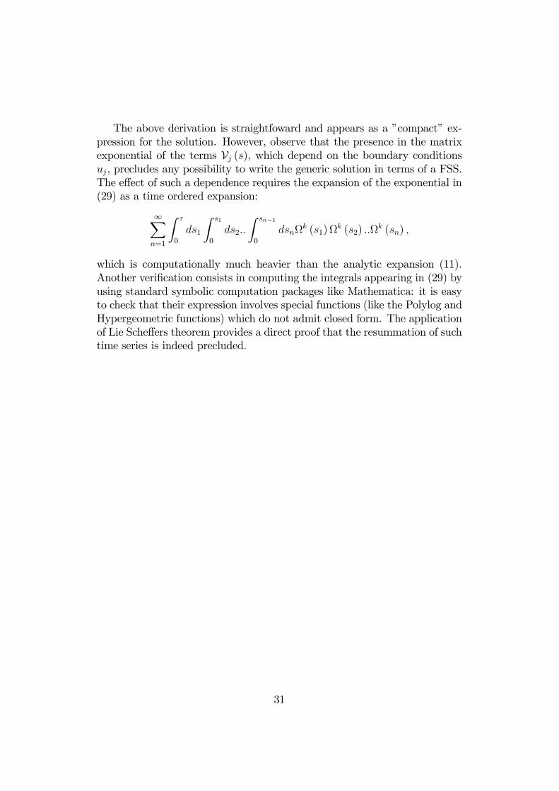
The above derivation is straightfoward and appears as a ”compact” ex-pression for the solution. However, observe that the presence in the matrixexponential of the terms Vj (s), which depend on the boundary conditionsuj, precludes any possibility to write the generic solution in terms of a FSS.The effect of such a dependence requires the expansion of the exponential in(29) as a time ordered expansion:

∞Xn=1

Z τ

0

ds1

Z s1

0

ds2..

Z sn−1

0

dsnΩk (s1)Ω

k (s2) ..Ωk (sn) ,

which is computationally much heavier than the analytic expansion (11).Another verification consists in computing the integrals appearing in (29) byusing standard symbolic computation packages like Mathematica: it is easyto check that their expression involves special functions (like the Polylog andHypergeometric functions) which do not admit closed form. The applicationof Lie Scheffers theorem provides a direct proof that the resummation of suchtime series is indeed precluded.

31