a comparison of affine region detectors
TRANSCRIPT
A Comparison of Affine Region Detectors
K. Mikolajczyk1, T. Tuytelaars2, C. Schmid4, A. Zisserman1,J. Matas3, F. Schaffalitzky1, T. Kadir1, L. Van Gool2
1 University of Oxford, OX1 3PJ Oxford, United Kingdom2 University of Leuven, Kasteelpark Arenberg 10, 3001 Leuven, Belgium
3 Czech Technical University, Karlovo Namesti 13, 121 35, Prague, Czech Republic4 INRIA, GRAVIR-CNRS, 655, av. de l’Europe, 38330 Montbonnot, France
[email protected], [email protected], [email protected],
[email protected], [email protected], [email protected],
[email protected], [email protected]
Abstract
The paper gives a snapshot of the state of the art in affine covariant region detectors, andcompares their performance on a set of test images under varying imaging conditions. Sixtypes of detectors are included: detectors based on affine normalization around Harris [23,33] and Hessian points [23], as proposed by Mikolajczyk and Schmid and by Schaffalitzkyand Zisserman; a detector of ‘maximally stable extremal regions’, proposed by Matas etal. [20]; an edge-based region detector [44] and a detector based on intensity extrema [46],proposed by Tuytelaars and Van Gool; and a detector of ‘salient regions’, proposed by Kadir,Zisserman and Brady [12]. The performance is measured against changes in viewpoint, scale,illumination, defocus and image compression.
The objective of this paper is also to establish a reference test set of images and perfor-mance software, so that future detectors can be evaluated in the same framework.
1 Introduction
Detecting regions covariant with a class of transformations has now reached some maturity in thecomputer vision literature. These regions have been used in quite varied applications including:wide baseline matching for stereo pairs [1, 20, 30, 46], reconstructing cameras for sets of disparateviews [33], image retrieval from large databases [35, 44], model based recognition [7, 18, 28, 31],object retrieval in video [38, 39], visual data mining [40], texture recognition [13, 14], shot lo-cation [34], robot localization [36] and servoing [45], building panoramas [2], symmetry detec-tion [43], and object categorization [4, 5, 6, 29].
In spite of theoretical basis for region detection the region is defined as the output of a detector.A region is therefore a set of pixels, which form a local image structure with some properties. Thisis different from classical segmentation, since the region boundaries do not have to correspondto changes in image appearance i.e., color, texture. The requirement of these regions is thatdetection should commute with the transformation, i.e., their shape is not fixed, but automaticallyadapts based on the underlying image intensities so as to always cover the same physical surface.As such, even though they have often been called invariant regions in the literature (e.g., [5, 13,40, 44]), in principle they should be termed covariant regions: the regions found in a picturedeformed by some transformation are the images of the regions found in the original picture,deformed under the same transformation. The confusion probably arises from the fact that, even
1

(a) (b) (c)
(d) (e) (f)
Figure 1: Class of transformations needed to cope with viewpoint changes. (a) Firstviewpoint; (b,c) second viewpoint. Fixed size circular patches (a,b) clearly do not suffice to dealwith general viewpoint changes. What is needed is an anisotropic rescaling, i.e., an affinity (c).Bottom row shows close-up of the images with surface corresponding patches.
though the regions themselves are covariant, the normalized image pattern they cover and thefeature descriptors derived from them are typically invariant.
For viewpoint changes the transformation of most interest is an affinity. This is illustrated infigure 1. Clearly, a region with fixed shape (a circular example is shown in figure 1(a) and (b))cannot cope with the geometric deformations caused by the change in viewpoint. We can observethat the circle doesn’t cover the same image content, i.e., the same physical surface. Instead,the shape of the region has to be adaptive, or covariant with respect to affinities (figure 1(c)– close-ups shown in figure 1(d)–(f)). Indeed, an affinity is sufficient to locally model imagedistortions arising from viewpoint changes, provided that (1) the scene surface can be locallyapproximated by a plane or in case of a rotating camera, and (2) ignoring perspective effects,which are typically small on a local scale anyway. Aside from the geometric deformations, alsophotometric deformations need to be taken into account. These can be modeled by a lineartransformation of the intensities.
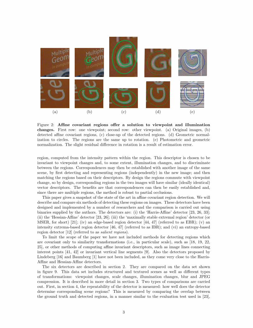
To further illustrate these concepts, and how affine covariant regions can be exploited to copewith the geometric and photometric deformation between wide baseline images, consider theexample shown in figure 2. Unlike the example of figure 1 (where a circular region was chosen forone viewpoint) the elliptical image regions here are detected independently in each viewpoint. Asis evident, the pre-image of these affine covariant regions correspond to the same surface region.Given such an affine covariant region, it is then possible to normalize against the geometric andphotometric deformations (shown in figure 2(d)(e)) and to obtain a viewpoint and illuminationinvariant description of the intensity pattern within the region.
In a typical matching application, the regions are used as follows. First, a set of covariantregions is detected in an image. Often a large number, perhaps hundreds or thousands, ofpossibly overlapping regions are obtained. A vector descriptor is then associated with each
2
(a) (b) (c) (d) (e)
Figure 2: Affine covariant regions offer a solution to viewpoint and illuminationchanges. First row: one viewpoint; second row: other viewpoint. (a) Original images, (b)detected affine covariant regions, (c) close-up of the detected regions. (d) Geometric normal-ization to circles. The regions are the same up to rotation. (e) Photometric and geometricnormalization. The slight residual difference in rotation is a result of estimation error.
region, computed from the intensity pattern within the region. This descriptor is chosen to beinvariant to viewpoint changes and, to some extent, illumination changes, and to discriminatebetween the regions. Correspondences may then be established with another image of the samescene, by first detecting and representing regions (independently) in the new image; and thenmatching the regions based on their descriptors. By design the regions commute with viewpointchange, so by design, corresponding regions in the two images will have similar (ideally identical)vector descriptors. The benefits are that correspondences can then be easily established and,since there are multiple regions, the method is robust to partial occlusions.
This paper gives a snapshot of the state of the art in affine covariant region detection. We willdescribe and compare six methods of detecting these regions on images. These detectors have beendesigned and implemented by a number of researchers and the comparison is carried out usingbinaries supplied by the authors. The detectors are: (i) the ‘Harris-Affine’ detector [23, 26, 33];(ii) the ‘Hessian-Affine’ detector [23, 26]; (iii) the ‘maximally stable extremal region’ detector (orMSER, for short) [21]; (iv) an edge-based region detector [44, 47] (referred to as EBR); (v) anintensity extrema-based region detector [46, 47] (referred to as IBR); and (vi) an entropy-basedregion detector [12] (referred to as salient regions).
To limit the scope of the paper we have not included methods for detecting regions whichare covariant only to similarity transformations (i.e., in particular scale), such as [18, 19, 22,25], or other methods of computing affine invariant descriptors, such as image lines connectinginterest points [41, 42] or invariant vertical line segments [9]. Also the detectors proposed byLindeberg [16] and Baumberg [1] have not been included, as they come very close to the Harris-Affine and Hessian-Affine detectors.
The six detectors are described in section 2. They are compared on the data set shownin figure 9. This data set includes structured and textured scenes as well as different typesof transformations: viewpoint changes, scale changes, illumination changes, blur and JPEGcompression. It is described in more detail in section 3. Two types of comparisons are carriedout. First, in section 4, the repeatability of the detector is measured: how well does the detectordetermine corresponding scene regions? This is measured by comparing the overlap betweenthe ground truth and detected regions, in a manner similar to the evaluation test used in [23],
3

but with special attention paid to the effect of the different scales (region sizes) of the variousdetectors’ output. Here, we also measure the accuracy of the regions shape, scale and localization.Second, the distinctiveness of the detected regions is assessed: how distinguishable are the regionsdetected? Following [24], we use the SIFT descriptor developed by Lowe [18], which is an 128-dimensional vector, to describe the intensity pattern within the image regions. This descriptorhas been demonstrated to be superior to others used in literature on a number of measures [24].
Our intention is that the images and tests described here will be a benchmark against whichfuture affine covariant region detectors can be assessed. The images, Matlab code to carry outthe performance tests, and binaries of the detectors are available fromhttp://www.robots.ox.ac.uk/˜vgg/research/affine.
2 Affine covariant detectors
In this section we give a brief description of the six region detectors used in the comparison.Section 2.1 describes the related methods Harris-Affine and Hessian-Affine. Sections 2.2 and 2.3describe methods for detecting edge-based regions and intensity extrema-based regions. Finally,sections 2.4 and 2.5 describe MSER and salient regions.
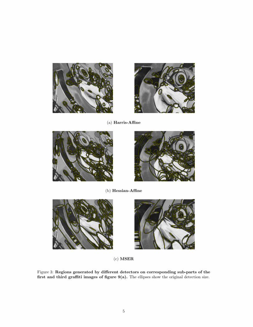
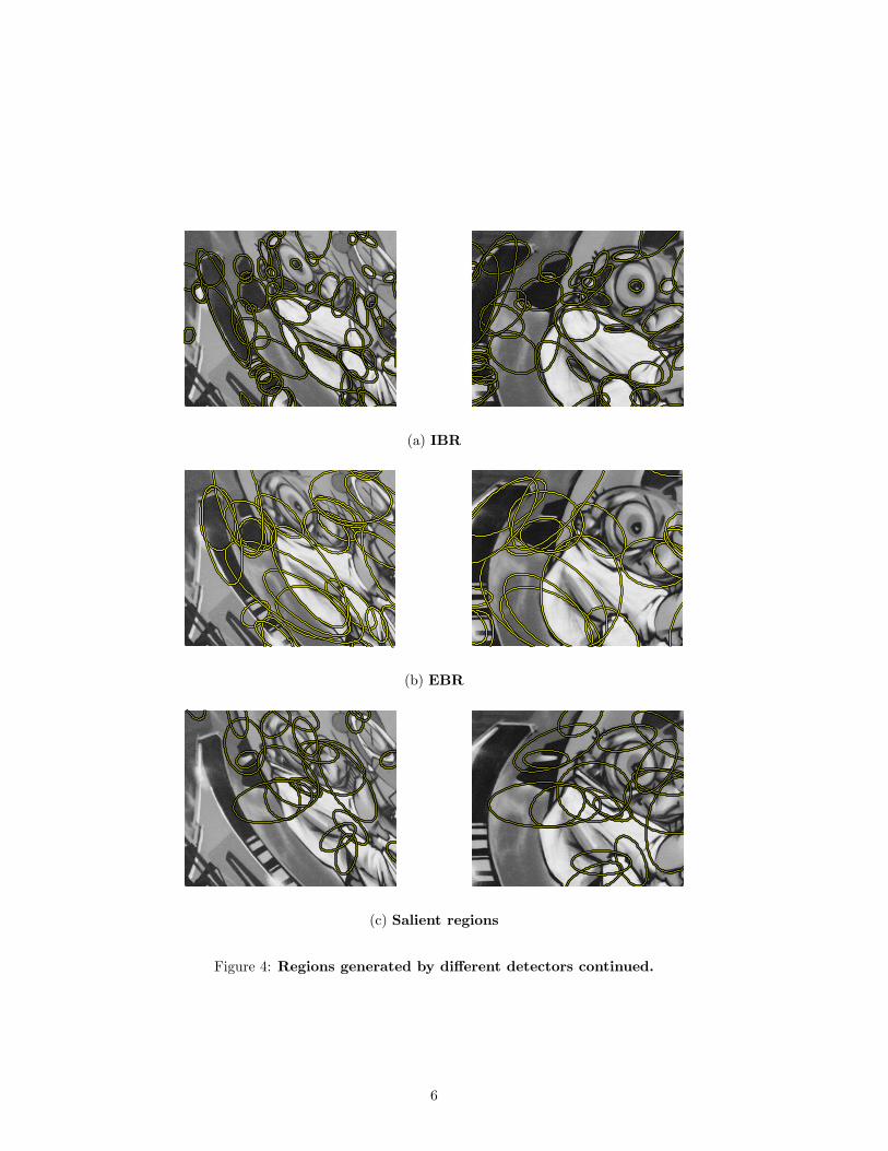
For the purpose of the comparisons the output region of all detector types are represented bya common shape, which is an ellipse. Figures 3 and 4 show the ellipses for all detectors on onepair of images. In order not to overload the images, only some of the corresponding regions thatwere actually detected in both images have been shown. This selection is obtained by increasingthe threshold.
In fact, for most of the detectors the output shape is an ellipse. However, for two of thedetectors (edge-based regions and MSER) it is not, and information is lost by this representation,as ellipses can only be matched up to a rotational degree of freedom. Examples of the originalregions detected by these two methods are given in figure 5. These are parallelogram-shapedregions for the edge-based region detector, and arbitrarily shaped regions for the MSER detector.In the following the representing ellipse is chosen to have the same first and second moments asthe originally detected region, which is an affine covariant construction method.
2.1 Detectors based on affine normalization – Harris-Affine & Hessian-Affine
We describe here two related methods which detect interest points in scale-space, and thendetermine an elliptical region for each point. Interest points are either detected with the Harrisdetector or with a detector based on the Hessian matrix. In both cases scale-selection is basedon the Laplacian, and the shape of the elliptical region is determined with the second momentmatrix of the intensity gradient [1, 16].
The second moment matrix, also called the auto-correlation matrix, is often used for featuredetection or for describing local image structures. Here it is used both in the Harris detectorand the elliptical shape estimation. This matrix describes the gradient distribution in a localneighborhood of a point:
M = µ(x, σI , σD) =[
µ11 µ12
µ21 µ22
]= σ2
D g(σI) ∗[
I2x(x, σD) IxIy(x, σD)
IxIy(x, σD) I2y (x, σD)
](1)
The local image derivatives are computed with Gaussian kernels of scale σD (differentiation scale).The derivatives are then averaged in the neighborhood of the point by smoothing with a Gaussianwindow of scale σI (integration scale). The eigenvalues of this matrix represent two principalsignal changes in a neighborhood of the point. This property enables the extraction of points,for which both curvatures are significant, that is the signal change is significant in orthogonaldirections. Such points are stable in arbitrary lighting conditions and are representative of animage. One of the most reliable interest point detectors, the Harris detector [10], is based on thisprinciple.
4
(a) Harris-Affine
(b) Hessian-Affine
(c) MSER
Figure 3: Regions generated by different detectors on corresponding sub-parts of thefirst and third graffiti images of figure 9(a). The ellipses show the original detection size.
5
(a) IBR
(b) EBR
(c) Salient regions
Figure 4: Regions generated by different detectors continued.
6

(a) EBR
(b) MSER
Figure 5: Originally detected region shapes for the regions shown in figures 3(c)and 4(a).
7
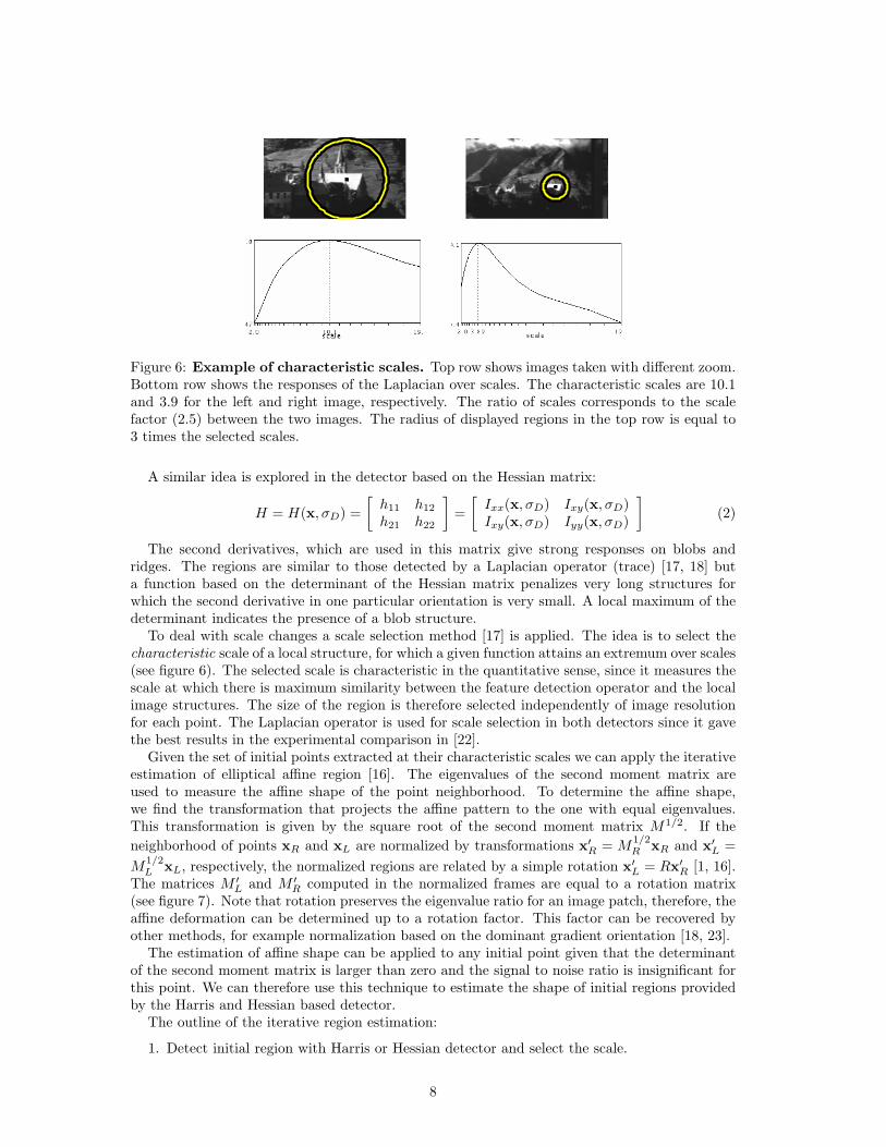
Figure 6: Example of characteristic scales. Top row shows images taken with different zoom.Bottom row shows the responses of the Laplacian over scales. The characteristic scales are 10.1and 3.9 for the left and right image, respectively. The ratio of scales corresponds to the scalefactor (2.5) between the two images. The radius of displayed regions in the top row is equal to3 times the selected scales.
A similar idea is explored in the detector based on the Hessian matrix:
H = H(x, σD) =[
h11 h12
h21 h22
]=
[Ixx(x, σD) Ixy(x, σD)Ixy(x, σD) Iyy(x, σD)
](2)
The second derivatives, which are used in this matrix give strong responses on blobs andridges. The regions are similar to those detected by a Laplacian operator (trace) [17, 18] buta function based on the determinant of the Hessian matrix penalizes very long structures forwhich the second derivative in one particular orientation is very small. A local maximum of thedeterminant indicates the presence of a blob structure.
To deal with scale changes a scale selection method [17] is applied. The idea is to select thecharacteristic scale of a local structure, for which a given function attains an extremum over scales(see figure 6). The selected scale is characteristic in the quantitative sense, since it measures thescale at which there is maximum similarity between the feature detection operator and the localimage structures. The size of the region is therefore selected independently of image resolutionfor each point. The Laplacian operator is used for scale selection in both detectors since it gavethe best results in the experimental comparison in [22].
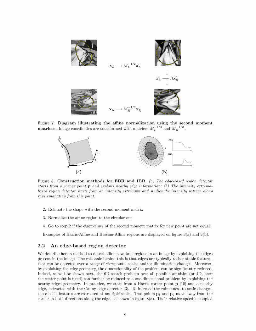
Given the set of initial points extracted at their characteristic scales we can apply the iterativeestimation of elliptical affine region [16]. The eigenvalues of the second moment matrix areused to measure the affine shape of the point neighborhood. To determine the affine shape,we find the transformation that projects the affine pattern to the one with equal eigenvalues.This transformation is given by the square root of the second moment matrix M1/2. If theneighborhood of points xR and xL are normalized by transformations x′R = M
1/2R xR and x′L =
M1/2L xL, respectively, the normalized regions are related by a simple rotation x′L = Rx′R [1, 16].
The matrices M ′L and M ′
R computed in the normalized frames are equal to a rotation matrix(see figure 7). Note that rotation preserves the eigenvalue ratio for an image patch, therefore, theaffine deformation can be determined up to a rotation factor. This factor can be recovered byother methods, for example normalization based on the dominant gradient orientation [18, 23].
The estimation of affine shape can be applied to any initial point given that the determinantof the second moment matrix is larger than zero and the signal to noise ratio is insignificant forthis point. We can therefore use this technique to estimate the shape of initial regions providedby the Harris and Hessian based detector.
The outline of the iterative region estimation:
1. Detect initial region with Harris or Hessian detector and select the scale.
8
xL −→ M−1/2L x′L
↓x′L −→ Rx′R
↓
xR −→ M−1/2R x′R
Figure 7: Diagram illustrating the affine normalization using the second momentmatrices. Image coordinates are transformed with matrices M
−1/2L and M
−1/2R .
p
p
p1
2
l
l1
2
qI(t)
f(t)
t
tt
(a) (b)
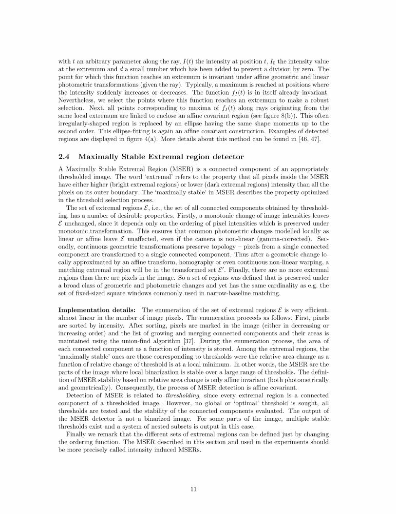
Figure 8: Construction methods for EBR and IBR. (a) The edge-based region detectorstarts from a corner point p and exploits nearby edge information; (b) The intensity extrema-based region detector starts from an intensity extremum and studies the intensity pattern alongrays emanating from this point.
2. Estimate the shape with the second moment matrix
3. Normalize the affine region to the circular one
4. Go to step 2 if the eigenvalues of the second moment matrix for new point are not equal.
Examples of Harris-Affine and Hessian-Affine regions are displayed on figure 3(a) and 3(b).
2.2 An edge-based region detector
We describe here a method to detect affine covariant regions in an image by exploiting the edgespresent in the image. The rationale behind this is that edges are typically rather stable features,that can be detected over a range of viewpoints, scales and/or illumination changes. Moreover,by exploiting the edge geometry, the dimensionality of the problem can be significantly reduced.Indeed, as will be shown next, the 6D search problem over all possible affinities (or 4D, oncethe center point is fixed) can further be reduced to a one-dimensional problem by exploiting thenearby edges geometry. In practice, we start from a Harris corner point p [10] and a nearbyedge, extracted with the Canny edge detector [3]. To increase the robustness to scale changes,these basic features are extracted at multiple scales. Two points p1 and p2 move away from thecorner in both directions along the edge, as shown in figure 8(a). Their relative speed is coupled
9

through the equality of relative affine invariant parameters l1 and l2:
li =∫
abs (|pi(1)(si) p− pi(si)|) dsi (3)
with si an arbitrary curve parameter (in both directions), pi(1)(si) the first derivative of pi(si)
with respect to si, abs() the absolute value and | . . . | the determinant. This condition prescribesthat the areas between the joint < p,p1 > and the edge and between the joint < p,p2 > andthe edge remain identical. This is an affine invariant criterion indeed. From now on, we simplyuse l when referring to l1 = l2.
For each value l, the two points p1(l) and p2(l) together with the corner p define a parallelo-gram Ω(l): the parallelogram spanned by the vectors p1(l)− p and p2(l)− p. This yields a onedimensional family of parallelogram-shaped regions as a function of l. From this 1D family weselect one (or a few) parallelogram for which the following photometric quantities of the texturego through an extremum.
Inv1 = abs(|p1 − pg p2 − pg||p− p1 p− p2|
)M1
00√M2
00M000 − (M1
00)2
Inv2 = abs(|p− pg q− pg||p− p1 p− p2|
)M1
00√M2
00M000 − (M1
00)2
with Mnpq =
∫Ω
In(x, y)xpyq dxdy
pg = (M1
10
M100
,M1
01
M100
) (4)
with Mnpq the nth order, (p + q)th degree moment computed over the region Ω(l), pg the center
of gravity of the region, weighted with intensity I(x, y), and q the corner of the parallelogramopposite to the corner point p (see figure 8(a)). The second factor in these formula has beenadded to ensure invariance under an intensity offset.
In the case of straight edges, the method described above cannot be applied, since l = 0along the entire edge. Since intersections of two straight edges occur quite often, we cannotsimply neglect this case. To circumvent this problem, the two photometric quantities given inEquation 4 are combined and locations where both functions reach a minimum value are takento fix the parameters s1 and s2 along the straight edges. Moreover, instead of relying on thecorrect detection of the Harris corner point, we can simply use the straight lines intersectionpoint instead. A more detailed explanation of this method can be found in [44, 47]. Examplesof detected regions are displayed in figure 5(a).
For easy comparison in the context of this paper, the parallelograms representing the invariantregions are replaced by the enclosed ellipses, as shown in figure 4(b). However, in this way theorientation-information is lost, so it should be avoided in a practical application, as discussed inthe begin of section 2.
2.3 Intensity extrema-based region detector
Here we describe a method to detect affine covariant regions that starts from intensity extrema(detected at multiple scales), and explores the image around them in a radial way, delineatingregions of arbitrary shape, which are then replaced by ellipses.
More precisely, given a local extremum in intensity, the intensity function along rays emanatingfrom the extremum is studied, as shown in figure 8(b). The following function is evaluated alongeach ray:
fI(t) =abs(I(t)− I0)
max( R t
0 abs(I(t)−I0)dt
t , d)
10
with t an arbitrary parameter along the ray, I(t) the intensity at position t, I0 the intensity valueat the extremum and d a small number which has been added to prevent a division by zero. Thepoint for which this function reaches an extremum is invariant under affine geometric and linearphotometric transformations (given the ray). Typically, a maximum is reached at positions wherethe intensity suddenly increases or decreases. The function fI(t) is in itself already invariant.Nevertheless, we select the points where this function reaches an extremum to make a robustselection. Next, all points corresponding to maxima of fI(t) along rays originating from thesame local extremum are linked to enclose an affine covariant region (see figure 8(b)). This oftenirregularly-shaped region is replaced by an ellipse having the same shape moments up to thesecond order. This ellipse-fitting is again an affine covariant construction. Examples of detectedregions are displayed in figure 4(a). More details about this method can be found in [46, 47].
2.4 Maximally Stable Extremal region detector
A Maximally Stable Extremal Region (MSER) is a connected component of an appropriatelythresholded image. The word ‘extremal’ refers to the property that all pixels inside the MSERhave either higher (bright extremal regions) or lower (dark extremal regions) intensity than all thepixels on its outer boundary. The ‘maximally stable’ in MSER describes the property optimizedin the threshold selection process.
The set of extremal regions E , i.e., the set of all connected components obtained by threshold-ing, has a number of desirable properties. Firstly, a monotonic change of image intensities leavesE unchanged, since it depends only on the ordering of pixel intensities which is preserved undermonotonic transformation. This ensures that common photometric changes modelled locally aslinear or affine leave E unaffected, even if the camera is non-linear (gamma-corrected). Sec-ondly, continuous geometric transformations preserve topology – pixels from a single connectedcomponent are transformed to a single connected component. Thus after a geometric change lo-cally approximated by an affine transform, homography or even continuous non-linear warping, amatching extremal region will be in the transformed set E ′. Finally, there are no more extremalregions than there are pixels in the image. So a set of regions was defined that is preserved undera broad class of geometric and photometric changes and yet has the same cardinality as e.g. theset of fixed-sized square windows commonly used in narrow-baseline matching.
Implementation details: The enumeration of the set of extremal regions E is very efficient,almost linear in the number of image pixels. The enumeration proceeds as follows. First, pixelsare sorted by intensity. After sorting, pixels are marked in the image (either in decreasing orincreasing order) and the list of growing and merging connected components and their areas ismaintained using the union-find algorithm [37]. During the enumeration process, the area ofeach connected component as a function of intensity is stored. Among the extremal regions, the‘maximally stable’ ones are those corresponding to thresholds were the relative area change as afunction of relative change of threshold is at a local minimum. In other words, the MSER are theparts of the image where local binarization is stable over a large range of thresholds. The defini-tion of MSER stability based on relative area change is only affine invariant (both photometricallyand geometrically). Consequently, the process of MSER detection is affine covariant.
Detection of MSER is related to thresholding, since every extremal region is a connectedcomponent of a thresholded image. However, no global or ‘optimal’ threshold is sought, allthresholds are tested and the stability of the connected components evaluated. The output ofthe MSER detector is not a binarized image. For some parts of the image, multiple stablethresholds exist and a system of nested subsets is output in this case.
Finally we remark that the different sets of extremal regions can be defined just by changingthe ordering function. The MSER described in this section and used in the experiments shouldbe more precisely called intensity induced MSERs.
11

2.5 Salient region detector
This detector is based on the pdf of intensity values computed over an elliptical region. Detectionproceeds in two steps: first, at each pixel the entropy of the pdf is evaluated over the threeparameter family of ellipses centred on that pixel. The set of entropy extrema over scale and thecorresponding ellipse parameters are recorded. These are candidate salient regions. Second, thecandidate salient regions over the entire image are ranked using the magnitude of the derivativeof the pdf with respect to scale. The top P ranked regions are retained.
In more detail, the elliptical region E centred on a pixel x is parameterized by its scale s(which specifies the major axis), its orientation θ (of the major axis), and the ratio of major tominor axes λ. The pdf of intensities p(I) is computed over E . The entropy H is then given by
H = −∑
I
p(I) log p(I)
The set of extrema over scale in H is computed for the parameters s, θ, λ for each pixel of theimage. For each extrema the derivative of the pdf p(I; s, θ, λ) with s is computed as
W =s2
2s− 1
∑I
|∂p(I; s, θ, λ)∂s
|,
and the saliency Y of the elliptical region is computed as Y = HW. The regions are ranked bytheir saliency Y. Examples of detected regions are displayed in figure 4(c). More details aboutthis method can be found in [12].
3 The image data set
Figure 9 shows examples from the image sets used to evaluate the detectors. Five differentchanges in imaging conditions are evaluated: viewpoint changes (a) & (b); scale changes (c) &(d); image blur (e) & (f); JPEG compression (g); and illumination (h). In the cases of viewpointchange, scale change and blur, the same change in imaging conditions is applied to two differentscene types. This means that the effect of changing the image conditions can be separatedfrom the effect of changing the scene type. One scene type contains homogeneous regions withdistinctive edge boundaries (e.g. graffiti, buildings), and the other contains repeated textures ofdifferent forms. These will be referred to as structured versus textured scenes respectively.
In the viewpoint change test the camera varies from a fronto-parallel view to one with sig-nificant foreshortening at approximately 60 degrees to the camera. The scale change and blursequences are acquired by varying the camera zoom and focus respectively. The scale changes byabout a factor of four. The light changes are introduced by varying the camera aperture. TheJPEG sequence is generated using a standard xv image browser with the image quality parametervarying from 40% to 2%. Each of the test sequences contains 6 images with a gradual geometricor photometric transformation. All images are of medium resolution (approximately 800 × 640pixels).
The images are either of planar scenes or the camera position is fixed during acquisition, sothat in all cases the images are related by homographies (plane projective transformations). Thismeans that the mapping relating images is known (or can be computed), and this mapping isused to determine ground truth matches for the affine covariant detectors.
The homographies between the reference (left most) image and the other images in a particulardataset are computed in two steps. First, a small number of point correspondences are selectedmanually between the reference and other image. These correspondences are used to compute anapproximate homography between the images, and the other image is warped by this homographyso that it is roughly aligned with the reference image. Second, a standard small-baseline robusthomography estimation algorithm is used to compute an accurate residual homography betweenthe reference and warped image (using hundreds of automatically detected and matched interest
12
points) [11]. The composition of these two homographies (approximate and residual) gives anaccurate homography between the reference and other image. The root-mean-square error is lessthan 1 pixel for every image pair.
Of course, the homography could be computed directly and automatically using correspon-dences of the affine covariant regions detected by any of the methods of section 2. The reason foradopting this two step approach is to have an estimation method independent of all the detectorsthat are being evaluated.
All the images as well as the computed homographies are available on the website.
3.1 Discussion
Before we compare the performance of the different detectors in more detail in the next section,a few more general observations can already be made, simply by examining the output of thedifferent detectors for the images shown in figures 3 and 4. For all our experiments (unlessexplicitly mentioned), the same set of parameters are used for each detector. These parametersare the default parameters given by the authors.
First of all, note that the ellipses in the left and right images of figures 3 and 4 do indeedcover more or less the same scene regions. This is the key requirement for covariant operators,and seems to be fulfilled for at least a subset of the detected regions for all detectors. Some otherkey observations are summarized below.
Complexity and required computation time: The computational complexity of the algo-rithm finding initial points in the Harris-Affine and Hessian-Affine detectors is O(n), where nis the number of pixels. The complexity of the automatic scale selection and shape adaptationalgorithm is O((m + k)p), where p is the number of initial points, m is a number of investigatedscales in the automatic scale selection and k is a number of iterations in the shape adaptationalgorithm.
For the intensity extrema-based region detector, the algorithm finding intensity extrema isO(n), where n is again the number of pixels. The complexity of constructing the actual regionaround the intensity extrema is O(p), where p is the number of intensity extrema.
For the edge-based region detector, the algorithm finding initial corner points and the algorithmfinding edges in the image are both O(n), where n is again the number of pixels. The complexityof constructing the actual region starting from the corners and edges is O(pd), where p is thenumber of corners and d is the average number of edges nearby a corner.
For the salient region detector, the complexity of the first step of the algorithm is O(nl),where l is the number of ellipses investigated at each pixel (the three discretized parameters ofthe ellipse shape). The complexity of the second step is O(e), where e is the number of extremadetected in the first step.
For the MSER detector, the computational complexity of the sorting step is O(n) if the rangeof image values is small, e.g. the typical 0, . . . , 255, since the sort can be implemented asbinsort. The complexity of the union-find algorithm is O(n log log n), i.e., fast.
Computation times vary widely, as can be seen in table 1. The computation times mentionedin this table have all been measured on a Pentium 4 2GHz Linux PC, for the leftmost image shownin figure 9(a), which is 800× 640 pixels. Even though the timings are for not heavily optimizedcode and may change depending on the implementation as well as on the image content, webelieve the table gives a reasonable indication of typical computation times.
Region density: The various detectors generate very different numbers of regions, c.f. table 1.The number of regions also strongly depends on the scene type, e.g. for the MSER detector thereare about 2600 regions for the textured blur scene (figure 9(f)) and only 230 for the light changescene (figure 9(h)). Similar behavior can be observed for other detectors.
The variation in numbers between detector type is to be expected since the detectors respondto different features and the images contain different numbers for a given feature type. For
13

(a)
(b)
(c)
(d)
(e) (f)
(g) (h)
Figure 9: Data set. (a), (b) Viewpoint change, (c),(d) Zoom+rotation, (e),(f) Image blur, (g)JPEG compression, (h) Light change. In the case of viewpoint change, scale change and blur,the same change in imaging conditions is applied to two different scene types: structured andtextured scenes. In the experimental comparisons, the left most image of each set is used as thereference image.
14

detector run time (min:sec) number of regionsHarris-Affine 0:01.43 1791Hessian-Affine 0:02.73 1649
MSER 0:00.66 533IBR 0:10.82 679EBR 2:44.59 1265
Salient Regions 33:33.89 513
Table 1: Computation times for the different detectors for the leftmost image of figure 9(a) (size800x640).
0 10 20 30 40 50 60 70 80 90 1000
50
100
150
200
250
300
350
400Histogram of detected region size
average region size
num
ber o
f det
ecte
d re
gion
s
0 10 20 30 40 50 60 70 80 90 1000
50
100
150
200
250
300
350
400Histogram of detected region size
average region size
num
ber o
f det
ecte
d re
gion
s
0 10 20 30 40 50 60 70 80 90 1000
20
40
60
80
100
120Histogram of detected region size
average region size
num
ber o
f det
ecte
d re
gion
s
Harris-Affine Hessian-Affine MSER
0 10 20 30 40 50 60 70 80 90 1000
10
20
30
40
50
60
70
80
90
100Histogram of detected region size
average region size
num
ber o
f det
ecte
d re
gion
s
0 10 20 30 40 50 60 70 80 90 1000
10
20
30
40
50
60
70
80
90Histogram of detected region size
average region size
num
ber o
f det
ecte
d re
gion
s
0 10 20 30 40 50 60 70 80 90 1000
20
40
60
80
100
120
140
160Histogram of detected region size
average region size
num
ber o
f det
ecte
d re
gion
s
IBR EBR Salient Regions
Figure 10: Histograms of region size for the different detectors for the reference imageof figure 9(a)). Note that the y axes do not have the same scalings in all cases.
example, the edge-based region detector requires curves, and if none of sufficient length occur ina particular image, then no regions of this type can be detected.
However, this variety is also a virtue: the different detectors are complementary. Some respondwell to structured scenes (e.g. MSER and the edge-based regions), others to more textured scenes(e.g. Harris-Affine and Hessian-Affine). We will return to this point in section 4.2.
Region size: Also the size of the detected regions significantly varies depending on the detector.Typically, Harris-Affine, Hessian-Affine and MSER detect many very small regions, whereas theother detectors only yield larger ones. This can also be seen in the examples shown in figures 3and 4. Figure 10 shows histograms of region size for the different region detectors. The size ofthe regions is measured as the geometric average of the half-length of both axes of the ellipses,which corresponds to the radius of a circular region with the same area. Larger regions typicallyhave a higher discriminative power, as they contain more information, which makes them easierto match, at the cost of a higher risk of being occluded or not covering a planar part of the scene.Also, as will be shown in the next section (cf. figure 11), large regions automatically have betterchances of overlapping other regions.
15
Distinguished regions versus measurement regions: As a final note, we would like todraw the attention of the reader to the fact that given a detected affine covariant region, it ispossible to associate with it any number of new affine regions that are obtained by affine covariantconstructions, such as scaling, taking the convex hull or fitting an ellipse based on second ordermoments. In this respect, one should make a distinction between a distinguished region and ameasurement region, as first pointed out in [20], where the former refers to the set of pixels thathave effectively contributed to the affine detector response while the latter can be any regionobtained by an affine covariant construction. Here, we focus on the original distinguished regions(except for the ellipse fitting for edge-based and MSER regions, to obtain the same shape for alldetectors), as they determine the intrinsic quality of a detector. In a practical matching setuphowever, it may be advantageous to use a different measurement region (see also section 5 andthe discussion on scale in next section).
4 Overlap comparison using homographies
The objective of this experiment is to measure the repeatability and accuracy of the detectors:to what extent do the detected regions overlap exactly the same scene area (i.e., are the pre-images identical)? How often are regions detected in one image without the corresponding regionbeing detected in another? Quantitative results are obtained by making these questions precise(see below). The ground truth in all cases is provided by mapping the regions detected on theimages in a set to a reference image using homographies. The basic measure of accuracy andrepeatability we use is the relative amount of overlap between the detected region in the referenceimage and the region detected in the other image, projected onto the reference image using thehomography relating the images. This gives a good indication of the chance that the region canbe matched correctly. In the tests the reference image is always the image of highest quality andis shown as the leftmost image of each set in figure 9.
Two important parameters characterize the performance of a region detector:
1. the repeatability, i.e., the average number of corresponding regions detected in images underdifferent geometric and photometric transformations, both in absolute and relative terms(i.e., percentage-wise), and
2. the accuracy of localization and region estimation.
However, before describing the overlap test in more detail, it is necessary to discuss the effectof region size and region density, since these affect the outcome of the overlap comparison.
A note on the effect of region size: Larger regions automatically have a better chance ofyielding good overlap scores. Simply rescaling the regions, i.e., using a different measurementregion (e.g. doubling the size of all regions) suffices to boost the overlap performance of a regiondetector. This can be understood as follows. Suppose the distinguished region is an ellipse,and the measurement region is also an ellipse centered on the distinguished region but with anarbitrary scaling s. Then from a geometrical point of view, varying the scaling defines a cone outof the image plane (with elliptical cross-section), and with s a distance on the cone axis. In thereference image there are two such cones – one from the distinguished region in that image, andthe other from the mapped distinguished region from the other image, as illustrated in figure 11.Clearly as the scaling goes to zero there is no intersection of the cones, and as the scaling goesto infinity the relative amount of overlap, defined as the ratio of the intersection to the union ofthe ellipses approaches unity.
To measure the intrinsic quality of a region detector, we need to define an overlap criterionthat is insensitive to such rescaling. Focusing on the original distinguished regions would unpro-portionally favour detectors with large distinguished regions. Instead, the solution adopted hereis to apply a scaling s that normalizes the reference region to a fixed region size prior to com-puting the overlap measure. It should be noted though that this is only for reason of comparison
16

Figure 11: Rescaling regions has an effect on their overlap.
of different detectors. It may result in increased or decreased repeatability scores compared towhat one might get in a typical matching experiment, where such normalization typically is notperformed (and is not desirable either).
A note on the effect of region density: Also the region density, i.e., the number of detectedregions per fixed amount of pixel area, may have an effect on the repeatability score of a detector.Indeed, if only a few regions are detected, the thresholds can be set very sharply, resulting in verystable regions, which typically perform better than average. At the other extreme, if the numberof regions becomes really huge, the image might get so cluttered with regions that some of themmay be matched by accident rather than by design. In the limit, one would get an (affine) scalespace approach rather than an affine covariant region detector.
One way out would be to tune the parameters of the detectors such that they all output asimilar number of regions. However, this is difficult to achieve in practice, since the numberof detected regions also depends on the scene type. Moreover, it is not straightforward for alldetectors to come up with a single parameter that can be varied to obtain the desired number ofregions in a meaningful way, i.e., representing some kind of ‘quality measure’ for the regions. Sowe use the default parameters supplied by the authors. To give an idea of the number of regions,both absolute and relative repeatability scores are given. In addition, for several detectors, therepeatability is computed versus the number of detected regions, which is reported in section 5.
4.1 Repeatability measure
Two regions are deemed to correspond if the overlap error, defined as the error in the imagearea covered by the regions, is sufficiently small:
1−Rµa ∩R(HT µbH)
(Rµa∪RHT µbH)
< εO
where Rµ represents the elliptic region defined by xT µx = 1. H is the homography relating thetwo images. The union of the regions is Rµa∪R(HT µbH), and Rµa∩R(HT µbH) is their intersection.The area of the union and the intersection of the regions are computed numerically.
The repeatability score for a given pair of images is computed as the ratio between thenumber of region-to-region correspondences and the smaller of the number of regions in the pair
17
≤5% 10% 20% 30% 40% 50% 60%
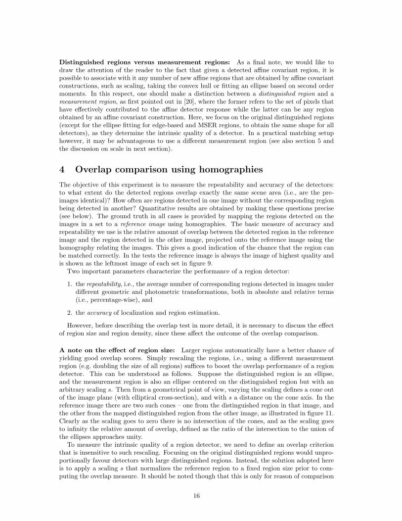
Figure 12: Overlap error εO. Examples of ellipses projected on the corresponding ellipse withthe ground truth transformation. (bottom) Overlap error for above displayed ellipses. Note thatthe overlap error comes from different size, orientation and position of the ellipses.
of images. We take into account only the regions located in the part of the scene present in bothimages.
To compensate for the effect of regions of different sizes, as mentioned in the previous section,we first rescale the regions as follows. Based on the region detected in the reference image, wedetermine the scale factor that transforms it into a region of normalized size (correspondingto a radius 30, in our experiments). Then, we apply this scale factor to both the region inthe reference image and the region detected in the other image which has been mapped ontothe reference image, before computing the actual overlap error as described above. The preciseprocedure is given in the Matlab code onhttp://www.robots.ox.ac.uk/~vgg/research/affine.
Examples of the overlap errors are displayed in figure 12. Note that an overlap error of 20%is very small as it corresponds to only 10% difference between the regions’ radius. Regions with50% overlap error can still be matched successfully with a robust descriptor.
4.2 Repeatability under various transformations
In a first set of experiments, we fix the overlap error threshold to 40% and the normalized regionsize to a radius of 30 pixels, and check the repeatability of the different region detectors forgradually increasing transformations, according to the image sets shown in figure 9. In otherwords, we measure how the number of correspondences depends on the transformation betweenthe reference and other images in the set. Both the relative and actual number of correspondingregions is recorded. In general we would like a detector to have a high repeatability score and alarge number of correspondences. This test allows to measure the robustness of the detectors tochanges in viewpoint, scale, illumination, etc.
The results of these tests are shown in figures 13-20(a) and (b). Figures 13-20(c) and (d)show matching results, which are discussed in section 5. A detailed discussion is given below,but we first make some general comments. The ideal plot for repeatability would be a horizontalline at 100%. As can be seen in all cases, neither a horizontal line nor 100% are achieved.Indeed the performance generally decreases with the severity of the transformation, and the bestperformance achieved is 95% for JPEG compression (figure 19). The reasons for this lack of100% performance are sometimes specific to detectors and scene types (discussed below), andsometimes general – the transformation is outside the range for which the detector is designed,e.g. discretization errors, noise, non-linear illumination changes, projective deformations etc. Alsothe limited ‘range’ of the regions shape (size, skewness, ...) can partially explain this effect. Forinstance, in case of a zoomed out test image, only the large regions in the reference image willsurvive the transformation, as the small regions will have become too small for accurate detection.The same holds for other types of transformations: very elongated regions in the reference imagemay become undetectable if the inferred affine transformation stretches them even further but,
18
on the other hand, allow for very large viewpoint changes if the inferred affine transformationmakes them rounder.
The left side of each figure typically represents small transformations. The repeatability scoreobtained in this range indicates how well a given detector performs for the given scene type andto what extent the detector is affected by a small transformation of this scene. The invarianceof the detector under the studied transformation, on the other hand, is reflected in the slope ofthe curves, i.e., how much does a given curve degrade with increasing transformations.
The absolute number of correspondences typically drops faster than the relative number. Thiscan be understood by the fact that in most cases larger transformations result in lower qualityimages and/or smaller commonly visible parts between the reference image and the other image,and hence a smaller number of regions are detected.
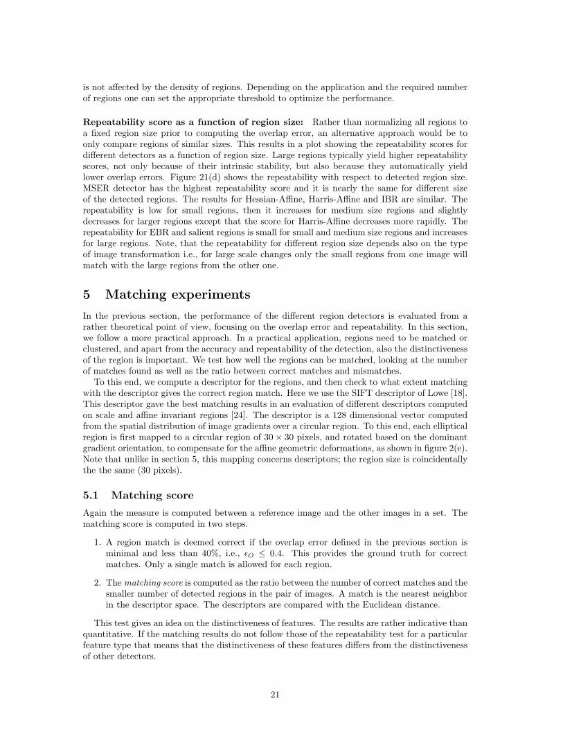
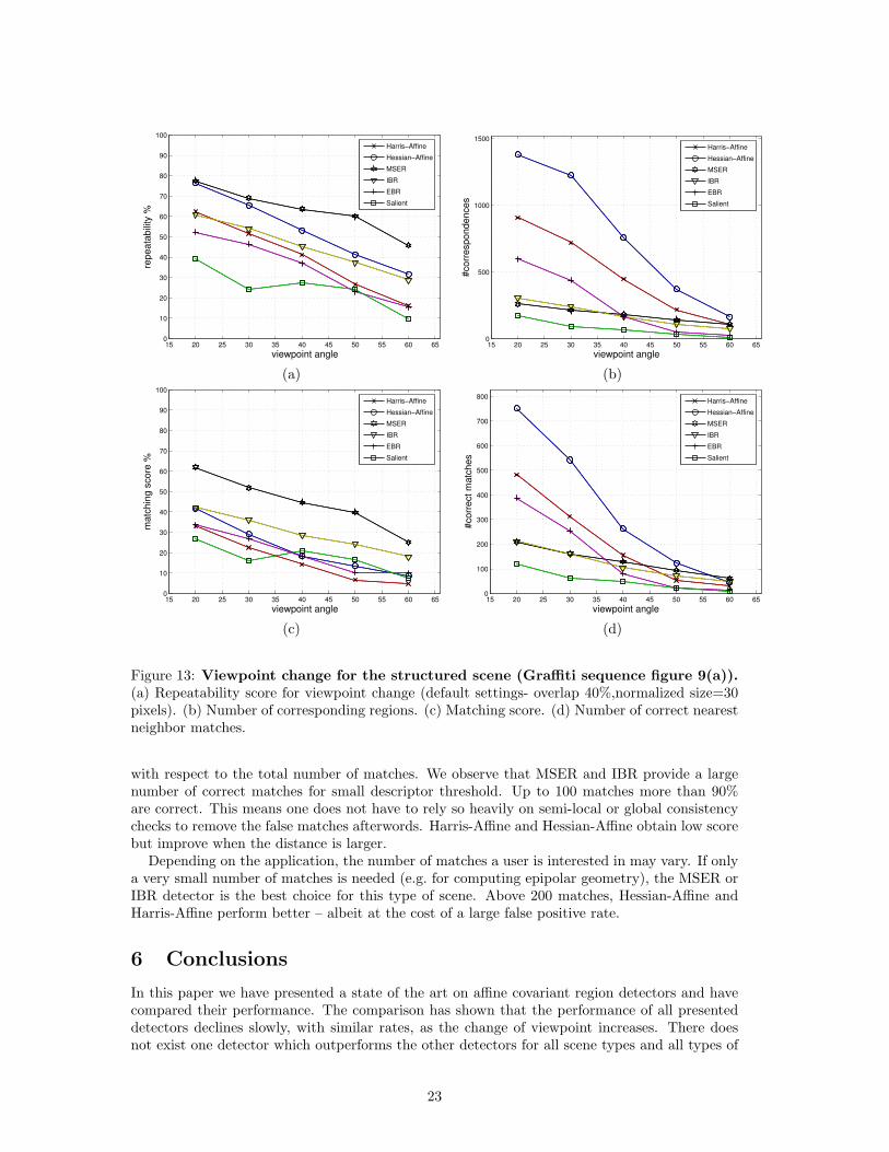
Viewpoint change: The effect of changing viewpoint for the structured graffiti scene fromfigure 9(a) are displayed in figure 13. Figure 13(a) shows the repeatability score and figure 13(b)the absolute number of correspondences. The results for images containing repeated texturemotifs (figure 9(b)) are displayed in figure 14. The best results are obtained with the MSERdetector for both scene types. This is due to the high detection accuracy especially on thehomogeneous regions with distinctive boundaries. The repeatability score for a viewpoint changeof 20 degrees varies between 40% and 78% and decreases for large viewpoint angles to 10%−46%.The largest number of corresponding regions is given by Hessian-Affine (1300) detector followedby Harris-Affine (900) detector for the structured scene, and given by Harris-Affine (1200), MSER(1200) and EBR (1300) detectors for the textured scene. These numbers decrease to less than200/400 for the structured/textured scene for large viewpoint angle.
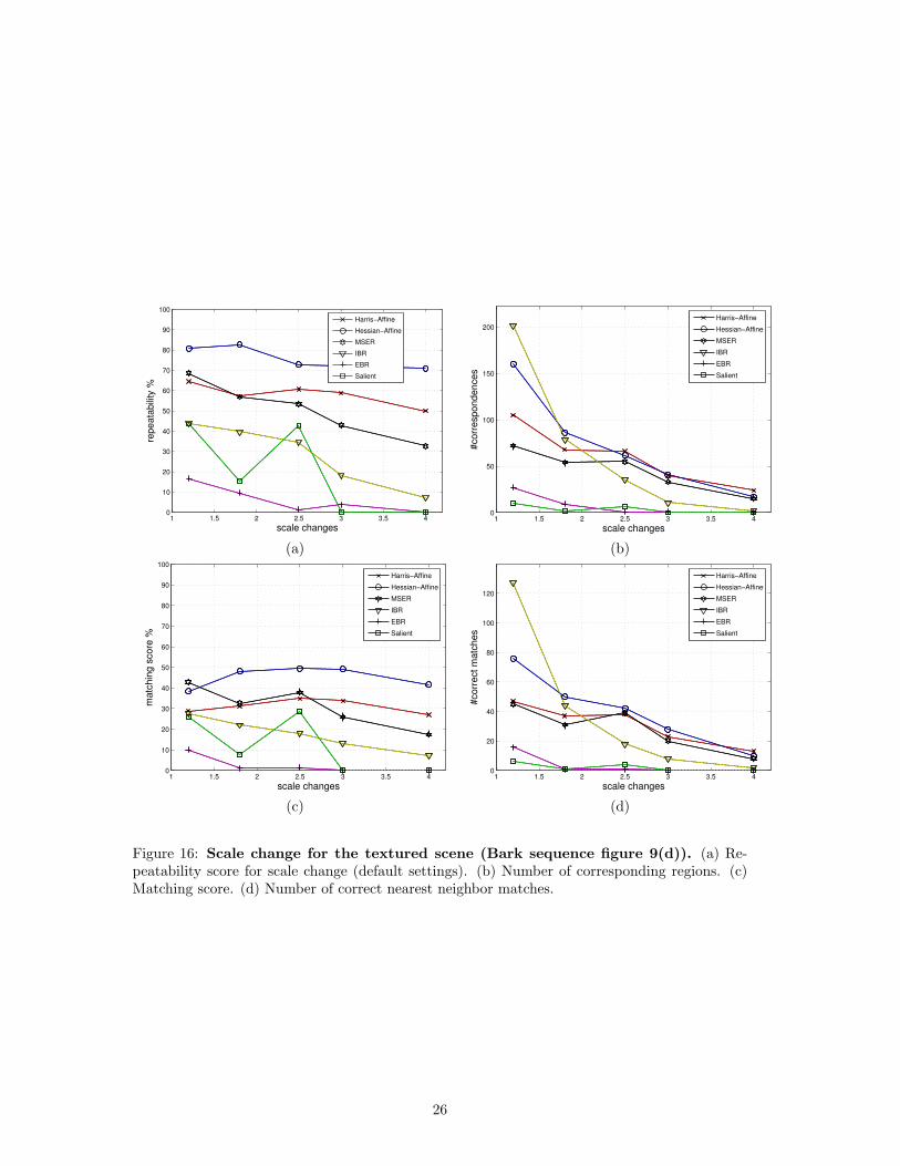
Scale change: Figure 15 shows the results for the structured scene from figure 9(c), whilefigure 16 shows the results for the textured scene from figure 9(d). The main image transformationis a scale change and in-plane rotation. The Hessian-Affine detector performs best, followed byMSER and Harris-Affine detectors. This confirms the high performance of the automatic scaleselection applied in both Hessian-Affine and Harris-Affine detectors. These plots clearly showthe sensitivity of the detectors to the scene type. For the textured scene, the edge-based regiondetector gives very low repeatability scores (below 20%), whereas for the structured scene, itsresults are similar to the other detectors, with score going from 60% down to 28%. The unstablerepeatability score of the salient region detector for the textured scene is due to the small numberof detected regions in this type of images.
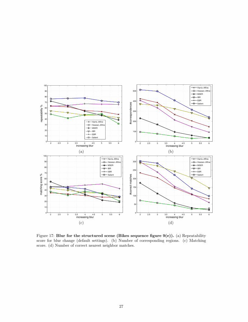
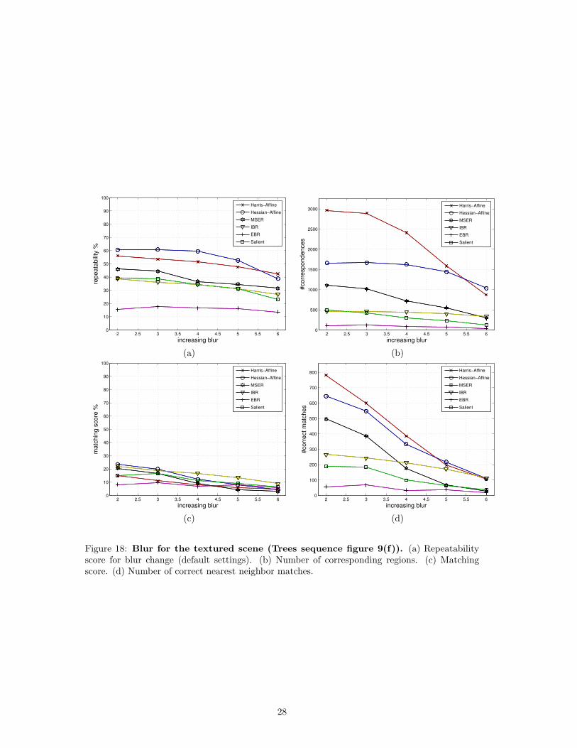
Blur: Figures 17 and 18 show the results for the structured scene from figure 9(e) and thetextured one from figure 9(f), both undergoing increasing amounts of image blur. The resultsare better than for viewpoint and scale changes, especially for the structured scene. All detectorshave nearly horizontal repeatability curves, showing a high level of invariance to image blur,except for the MSER detector, which is clearly more sensitive to this type of transformation.This is because the region boundaries become smooth, and the segmentation process is lessaccurate. The number of corresponding regions detected on structured scene is much lower thanfor the textured scene and it changes by a different factor for different detectors. This clearlyshows that the detectors respond to different features. The repeatability for the EBR detectoris very low for the textured scene. This can be explained by the lack of stable edges, on whichthe region extraction is based.
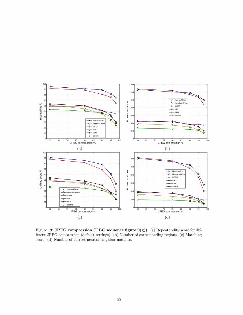
JPEG artifacts: Figure 19 shows the score for the JPEG compression sequence from fig-ure 9(g). For this type of structured scene (buildings), with large homogeneous areas and dis-tinctive corners, Hessian-Affine and Harris-Affine are clearly best suited. The degradation underincreasing compression artefacts is similar for all detectors.
19
Light change: Figure 20 shows the results for light changes for the images on figure 9(h).All curves are nearly horizontal, showing good robustness to illumination changes, although theMSER obtains the highest repeatability score for this type of scene. The absolute score shows howa small transformation of this type of a scene can affect the repeatability of different detectors.
General conclusions: For most experiments the MSER regions or Hessian-Affine obtain thebest repeatability score and are followed by Harris-Affine. Salient regions give relatively lowrepeatability. For the edge-based region detector, it largely depends on the scene content, i.e.,whether the image contains stable curves or not. The intensity extrema-based region detectorgives average scores. Results largely depend on the type of scene used for the experiments. Again,this illustrates the complementarity of the various detectors. Depending on the application, acombination of detectors is probably prudent.
Viewpoint changes are the most difficult type of transformation to cope with, followed by scalechanges. All detectors behave more or less similar under the different types of transformations,except for the blur sequence of figure 17, where MSER performs significantly worse than theothers.
In the majority of the examples Hessian-Affine and Harris-Affine detector provide severaltimes more corresponding regions than the other detectors. The Hessian-Affine detector almostsystematically outperforms the Harris-Affine detector, and the same holds for MSER with respectto IBR.
4.3 More detailed tests
To further validate our experimental setup and to obtain a deeper insight in what is actuallygoing on, a more detailed analysis is performed on one image pair with a viewpoint change of 40degrees, namely the first and third column of the graffiti sequence shown in figure 9(a).
Accuracy of the detectors: First, we test the effect of our choice for the overlap errorthreshold. This was fixed to 40% in all the previous experiments. Choosing a lower thresholdresults in more accurate regions, (see figure 12). Figure 21(a) shows the repeatability scoreas a function of the overlap error. Clearly, as the required overlap is relaxed, more regions arequalified as corresponding, and the repeatability scores go up. The relative ordering of the variousdetectors remains virtually the same, except for the Harris-Affine and Hessian region detectors.They improve their ranking with increasing overlap error, which means that these detectors areless accurate than the others – at least for this type of scene.
Choice of normalized region size: Next, we test the effect of our choice of the normalizedregion size. This was fixed to a radius of 30 pixels in all the previous experiments. Figure 21(b)shows how the repeatability scores vary as a function of the normalized region size, with theoverlap error threshold fixed to 40%. The relative ordering of the different detectors stays thesame, which indicates that our experimental setup is not very sensitive to the choice of thenormalized region size. With a larger normalized region size, we obtain lower overlap errors andthe curves increase slightly (see also figure 11).
Varying the region density: For some detectors, it is possible to vary the number of detectedregions, simply by changing the value of one significant parameter. This makes it possible tocompensate for the effect that different region densities might have on the repeatability scoresand compare different detectors when they output similar number of regions. Figure 21(c) showsthat the repeatability of MSER (98%) and IBR (70%) is high for a small number of regions (70)and decreases to 63% and 53% respectively for 350 detected regions, unlike the repeatabilityfor salient regions which is stable for a small number of regions and slightly increases for morethan 300 regions. However, the rank of the detectors remains the same in the range of availablethreshold settings, therefore the order of the detectors in the experiments in the previous section
20
is not affected by the density of regions. Depending on the application and the required numberof regions one can set the appropriate threshold to optimize the performance.
Repeatability score as a function of region size: Rather than normalizing all regions toa fixed region size prior to computing the overlap error, an alternative approach would be toonly compare regions of similar sizes. This results in a plot showing the repeatability scores fordifferent detectors as a function of region size. Large regions typically yield higher repeatabilityscores, not only because of their intrinsic stability, but also because they automatically yieldlower overlap errors. Figure 21(d) shows the repeatability with respect to detected region size.MSER detector has the highest repeatability score and it is nearly the same for different sizeof the detected regions. The results for Hessian-Affine, Harris-Affine and IBR are similar. Therepeatability is low for small regions, then it increases for medium size regions and slightlydecreases for larger regions except that the score for Harris-Affine decreases more rapidly. Therepeatability for EBR and salient regions is small for small and medium size regions and increasesfor large regions. Note, that the repeatability for different region size depends also on the typeof image transformation i.e., for large scale changes only the small regions from one image willmatch with the large regions from the other one.
5 Matching experiments
In the previous section, the performance of the different region detectors is evaluated from arather theoretical point of view, focusing on the overlap error and repeatability. In this section,we follow a more practical approach. In a practical application, regions need to be matched orclustered, and apart from the accuracy and repeatability of the detection, also the distinctivenessof the region is important. We test how well the regions can be matched, looking at the numberof matches found as well as the ratio between correct matches and mismatches.
To this end, we compute a descriptor for the regions, and then check to what extent matchingwith the descriptor gives the correct region match. Here we use the SIFT descriptor of Lowe [18].This descriptor gave the best matching results in an evaluation of different descriptors computedon scale and affine invariant regions [24]. The descriptor is a 128 dimensional vector computedfrom the spatial distribution of image gradients over a circular region. To this end, each ellipticalregion is first mapped to a circular region of 30× 30 pixels, and rotated based on the dominantgradient orientation, to compensate for the affine geometric deformations, as shown in figure 2(e).Note that unlike in section 5, this mapping concerns descriptors; the region size is coincidentallythe the same (30 pixels).
5.1 Matching score
Again the measure is computed between a reference image and the other images in a set. Thematching score is computed in two steps.
1. A region match is deemed correct if the overlap error defined in the previous section isminimal and less than 40%, i.e., εO ≤ 0.4. This provides the ground truth for correctmatches. Only a single match is allowed for each region.
2. The matching score is computed as the ratio between the number of correct matches and thesmaller number of detected regions in the pair of images. A match is the nearest neighborin the descriptor space. The descriptors are compared with the Euclidean distance.
This test gives an idea on the distinctiveness of features. The results are rather indicative thanquantitative. If the matching results do not follow those of the repeatability test for a particularfeature type that means that the distinctiveness of these features differs from the distinctivenessof other detectors.
21

The effect of rescaling the regions: Here, the issue arises on what scale to compute thedescriptor for a given region. Indeed, rather than taking the original distinguished region, onemight also rescale the region first, which typically leads to more discriminative power – certainlyfor the small regions. Figure 22(c) shows how the matching score for the different detectors variesfor different scale factors. Typically, the curves go slightly up for larger measurement regions,except for EBR and salient regions which attain their maximum score for scale factor of 2 and3 respectively. However, except for EBR the relative ordering of the different detectors remainsunaltered. For all our matching experiments, we selected a scale factor of 3.
It should be noted though that in a practical application a large scale factor can be moredetrimental, due to the higher risk of occlusions or non-planarities. Since in our experimentalsetup all images are related by homographies, these effects do not occur.
5.2 Matching under various transformations
Figures 13 - 20 (c) and (d) give the results of the matching experiment for the different typesof transformations. These are basically the same plots as given in figures 13 - 20 (a) and (b)but now focusing on regions that have actually been matched, rather than just correspondingregions.
For most transformations, the plots look indeed very similar to (albeit a bit lower than)the results obtained with the overlap error test. This indicates that the regions typically havesufficient distinctiveness to be matched automatically. One should be careful though to generalizethese results because these might be statistically unreliable, e.g. for much larger number offeatures in database retrieval.
Sometimes, the score or relative ordering of the detectors differs significantly from the overlaperror tests of the previous section (e.g. figures 17 and 20). This means that the regions found bysome detectors are not distinctive and many mismatches occur.
The ranking of the detectors changes in figure 20(c) comparing to figure 20(a) which meansthe Harris-Affine and Hessian-Affine are less distinctive. These detectors find several slightlydifferent regions containing the same local structure all of which have a small overlap error.Thus, the matched regions might have the overlap smaller than 40% but the minimum overlaperror is for a slightly different region. In this way the matched regions are counted as incorrect.The same change in ranking for Harris-Affine and Hessian-Affine can be observed on the resultsfor other transformations. However the rank of the figures (d) showing the number of matchedregions do not change with respect to the number of corresponding regions on figures (b).
The curves for figure 18(c) and (d) give the results for the textured scene shown in figure 9(f).For this case, the matching scores are significantly lower than the repeatability scores obtainedearlier. This can be explained by the fact that the scene contains many similar local structures,that can hardly be distinguished.
Ratio between correct and false matches: So far, we investigated the matching capabilityof corresponding regions. In a typical matching application, what matters is the ratio betweencorrect matches and false matches, i.e., are the regions within a correct match more similar toeach other than two regions that do not correspond but accidentally look more or less similar ?Here, the accuracy of the region detection plays a role, as does the variability of the intensitypatterns for all regions found by a detector i.e., the distinctiveness. Figure 22(a) shows thepercentage of correct matches as a function of the number of matches. A match is the nearestneighbor in the SIFT feature space. These curves were obtained by ranking the matches based onthe distance between the nearest neighbors. To obtain the same number of matches for differentdetectors the threshold was individually changed for each region type.
As the threshold, therefore the number of matches increases (figure 22(a)), the number ofcorrect as well as false matches also increases, but the number of false matches increases faster,hence the percentage of correct matches drops. For a good detector, a small threshold results inalmost exclusively correct matches. Figure 22(b) shows the absolute number of correct matches
22
15 20 25 30 35 40 45 50 55 60 650
10
20
30
40
50
60
70
80
90
100
viewpoint angle
repe
atab
ility
%Harris−Affine
Hessian−Affine
MSER
IBR
EBR
Salient
15 20 25 30 35 40 45 50 55 60 650
500
1000
1500
viewpoint angle
#cor
resp
onde
nces
Harris−Affine
Hessian−Affine
MSER
IBR
EBR
Salient
(a) (b)
15 20 25 30 35 40 45 50 55 60 650
10
20
30
40
50
60
70
80
90
100
viewpoint angle
mat
chin
g sc
ore
%
Harris−Affine
Hessian−Affine
MSER
IBR
EBR
Salient
15 20 25 30 35 40 45 50 55 60 650
100
200
300
400
500
600
700
800
viewpoint angle
#cor
rect
mat
ches
Harris−Affine
Hessian−Affine
MSER
IBR
EBR
Salient
(c) (d)
Figure 13: Viewpoint change for the structured scene (Graffiti sequence figure 9(a)).(a) Repeatability score for viewpoint change (default settings- overlap 40%,normalized size=30pixels). (b) Number of corresponding regions. (c) Matching score. (d) Number of correct nearestneighbor matches.
with respect to the total number of matches. We observe that MSER and IBR provide a largenumber of correct matches for small descriptor threshold. Up to 100 matches more than 90%are correct. This means one does not have to rely so heavily on semi-local or global consistencychecks to remove the false matches afterwords. Harris-Affine and Hessian-Affine obtain low scorebut improve when the distance is larger.
Depending on the application, the number of matches a user is interested in may vary. If onlya very small number of matches is needed (e.g. for computing epipolar geometry), the MSER orIBR detector is the best choice for this type of scene. Above 200 matches, Hessian-Affine andHarris-Affine perform better – albeit at the cost of a large false positive rate.
6 Conclusions
In this paper we have presented a state of the art on affine covariant region detectors and havecompared their performance. The comparison has shown that the performance of all presenteddetectors declines slowly, with similar rates, as the change of viewpoint increases. There doesnot exist one detector which outperforms the other detectors for all scene types and all types of
23
15 20 25 30 35 40 45 50 55 60 650
10
20
30
40
50
60
70
80
90
100
viewpoint angle
repe
atab
ility
%
Harris−Affine
Hessian−Affine
MSER
IBR
EBR
Salient
15 20 25 30 35 40 45 50 55 60 650
200
400
600
800
1000
1200
1400
viewpoint angle
#cor
resp
onde
nces
Harris−Affine
Hessian−Affine
MSER
IBR
EBR
Salient
(a) (b)
15 20 25 30 35 40 45 50 55 60 650
10
20
30
40
50
60
70
80
90
100
viewpoint angle
mat
chin
g sc
ore
%
Harris−Affine
Hessian−Affine
MSER
IBR
EBR
Salient
15 20 25 30 35 40 45 50 55 60 650
100
200
300
400
500
600
700
800
900
1000
viewpoint angle
#cor
rect
mat
ches
Harris−Affine
Hessian−Affine
MSER
IBR
EBR
Salient
(c) (d)
Figure 14: Viewpoint change for the textured scene (Wall sequence figure 9(b)). (a)Repeatability score for viewpoint change (default settings). (b) Number of corresponding regions.(c) Matching score. (d) Number of correct nearest neighbor matches.
24

1 1.2 1.4 1.6 1.8 2 2.2 2.4 2.6 2.8 30
10
20
30
40
50
60
70
80
90
100
scale changes
repe
atab
ility
%
Harris−Affine
Hessian−Affine
MSER
IBR
EBR
Salient
1 1.2 1.4 1.6 1.8 2 2.2 2.4 2.6 2.8 30
200
400
600
800
1000
1200
1400
1600
scale changes
#cor
resp
onde
nces
Harris−Affine
Hessian−Affine
MSER
IBR
EBR
Salient
(a) (b)
1 1.2 1.4 1.6 1.8 2 2.2 2.4 2.6 2.8 30
10
20
30
40
50
60
70
80
90
100
scale changes
mat
chin
g sc
ore
%
Harris−Affine
Hessian−Affine
MSER
IBR
EBR
Salient
1 1.2 1.4 1.6 1.8 2 2.2 2.4 2.6 2.8 30
100
200
300
400
500
600
700
800
900
scale changes
#cor
rect
mat
ches
Harris−Affine
Hessian−Affine
MSER
IBR
EBR
Salient
(c) (d)
Figure 15: Scale change for the structured scene (Boat sequence figure 9(c)). (a)Repeatability score for scale change (default settings). (b) Number of corresponding regions. (c)Matching score. (d) Number of correct nearest neighbor matches.
25
1 1.5 2 2.5 3 3.5 40
10
20
30
40
50
60
70
80
90
100
scale changes
repe
atab
ility
%
Harris−Affine
Hessian−Affine
MSER
IBR
EBR
Salient
1 1.5 2 2.5 3 3.5 40
50
100
150
200
scale changes
#cor
resp
onde
nces
Harris−Affine
Hessian−Affine
MSER
IBR
EBR
Salient
(a) (b)
1 1.5 2 2.5 3 3.5 40
10
20
30
40
50
60
70
80
90
100
scale changes
mat
chin
g sc
ore
%
Harris−Affine
Hessian−Affine
MSER
IBR
EBR
Salient
1 1.5 2 2.5 3 3.5 40
20
40
60
80
100
120
scale changes
#cor
rect
mat
ches
Harris−Affine
Hessian−Affine
MSER
IBR
EBR
Salient
(c) (d)
Figure 16: Scale change for the textured scene (Bark sequence figure 9(d)). (a) Re-peatability score for scale change (default settings). (b) Number of corresponding regions. (c)Matching score. (d) Number of correct nearest neighbor matches.
26
2 2.5 3 3.5 4 4.5 5 5.5 60
10
20
30
40
50
60
70
80
90
100
increasing blur
repe
atab
ility
%
Harris−Affine
Hessian−Affine
MSER
IBR
EBR
Salient
2 2.5 3 3.5 4 4.5 5 5.5 60
100
200
300
400
500
increasing blur
#cor
resp
onde
nces
Harris−Affine
Hessian−Affine
MSER
IBR
EBR
Salient
(a) (b)
2 2.5 3 3.5 4 4.5 5 5.5 60
10
20
30
40
50
60
70
80
90
100
increasing blur
mat
chin
g sc
ore
%
Harris−Affine
Hessian−Affine
MSER
IBR
EBR
Salient
2 2.5 3 3.5 4 4.5 5 5.5 60
50
100
150
200
250
300
increasing blur
#cor
rect
mat
ches
Harris−Affine
Hessian−Affine
MSER
IBR
EBR
Salient
(c) (d)
Figure 17: Blur for the structured scene (Bikes sequence figure 9(e)). (a) Repeatabilityscore for blur change (default settings). (b) Number of corresponding regions. (c) Matchingscore. (d) Number of correct nearest neighbor matches.
27
2 2.5 3 3.5 4 4.5 5 5.5 60
10
20
30
40
50
60
70
80
90
100
increasing blur
repe
atab
ility
%
Harris−Affine
Hessian−Affine
MSER
IBR
EBR
Salient
2 2.5 3 3.5 4 4.5 5 5.5 60
500
1000
1500
2000
2500
3000
increasing blur
#cor
resp
onde
nces
Harris−Affine
Hessian−Affine
MSER
IBR
EBR
Salient
(a) (b)
2 2.5 3 3.5 4 4.5 5 5.5 60
10
20
30
40
50
60
70
80
90
100
increasing blur
mat
chin
g sc
ore
%
Harris−Affine
Hessian−Affine
MSER
IBR
EBR
Salient
2 2.5 3 3.5 4 4.5 5 5.5 60
100
200
300
400
500
600
700
800
increasing blur
#cor
rect
mat
ches
Harris−Affine
Hessian−Affine
MSER
IBR
EBR
Salient
(c) (d)
Figure 18: Blur for the textured scene (Trees sequence figure 9(f)). (a) Repeatabilityscore for blur change (default settings). (b) Number of corresponding regions. (c) Matchingscore. (d) Number of correct nearest neighbor matches.
28
60 65 70 75 80 85 90 95 1000
10
20
30
40
50
60
70
80
90
100
JPEG compression %
repe
atab
ility
%
Harris−Affine
Hessian−Affine
MSER
IBR
EBR
Salient
60 65 70 75 80 85 90 95 1000
200
400
600
800
1000
1200
1400
JPEG compression %
#cor
resp
onde
nces
Harris−Affine
Hessian−Affine
MSER
IBR
EBR
Salient
(a) (b)
60 65 70 75 80 85 90 95 1000
10
20
30
40
50
60
70
80
90
100
JPEG compression %
mat
chin
g sc
ore
%
Harris−Affine
Hessian−Affine
MSER
IBR
EBR
Salient
60 65 70 75 80 85 90 95 1000
200
400
600
800
1000
1200
JPEG compression %
#cor
rect
mat
ches Harris−Affine
Hessian−Affine
MSER
IBR
EBR
Salient
(c) (d)
Figure 19: JPEG compression (UBC sequence figure 9(g)). (a) Repeatability score for dif-ferent JPEG compression (default settings). (b) Number of corresponding regions. (c) Matchingscore. (d) Number of correct nearest neighbor matches.
29

2 2.5 3 3.5 4 4.5 5 5.5 60
10
20
30
40
50
60
70
80
90
100
decreasing light
repe
atab
ility
%
Harris−Affine
Hessian−Affine
MSER
IBR
EBR
Salient
2 2.5 3 3.5 4 4.5 5 5.5 60
100
200
300
400
500
600
decreasing light
#cor
resp
onde
nces
Harris−Affine
Hessian−Affine
MSER
IBR
EBR
Salient
(a) (b)
2 2.5 3 3.5 4 4.5 5 5.5 60
10
20
30
40
50
60
70
80
90
100
decreasing light
mat
chin
g sc
ore
%
Harris−Affine
Hessian−Affine
MSER
IBR
EBR
Salient
2 2.5 3 3.5 4 4.5 5 5.5 60
50
100
150
200
250
300
350
decreasing light
#cor
rect
mat
ches
Harris−Affine
Hessian−Affine
MSER
IBR
EBR
Salient
(c) (d)
Figure 20: Illumination change (Leuven sequence figure 9(h)). (a) Repeatability scorefor different illumination (default settings). (b) Number of corresponding regions. (c) Matchingscore. (d) Number of correct nearest neighbor matches.
30

10 20 30 40 50 600
10
20
30
40
50
60
70
80
90
100
overlap error %
repe
atab
ility
%
Harris−Affine
Hessian−Affine
MSER
IBR
EBR
Salient
10 20 30 40 50 60 70 80 90 100 110 1200
10
20
30
40
50
60
70
80
90
100
normalized region size
repe
atab
ility
%
Harris−Affine
Hessian−Affine
MSER
IBR
EBR
Salient
(a) (b)
0 100 200 300 400 500 600 700 8000
10
20
30
40
50
60
70
80
90
100
number of detected regions
repe
atab
ility
%
MSER
IBR
Salient
0 10 20 30 40 50 600
10
20
30
40
50
60
70
80
90
100
region size
repe
atab
ility
%
Harris−Affine
Hessian−Affine
MSER
IBR
EBR
Salient
(c) (d)
Figure 21: Viewpoint change (Graffiti image pair - 1st and 3rd column in figure 9(a)).(a) Repeatability score for different overlap error for one pair (normalized size=30 pixels) . (b) Re-peatability score for different normalized region size (overlap error < 40%). (c) Repeatabilityscore for different number of detected regions (overlap error= 40%, normalized size=30 pixels).(d) Repeatability score as a function of region size.
31

0 50 100 150 200 250 300 350 400 4500
10
20
30
40
50
60
70
80
90
100
110
total number of matches
corr
ect m
atch
es %
Harris−Affine
Hessian−Affine
MSER
IBR
EBR
Salient
0 50 100 150 200 250 300 350 400 450 5000
20
40
60
80
100
120
140
160
180
200
total number of matches
corr
ect m
atch
es
Harris−Affine
Hessian−Affine
MSER
IBR
EBR
Salient
(a) (b)
1 1.5 2 2.5 3 3.5 4 4.5 50
10
20
30
40
50
60
70
80
90
100
region size factor
mat
chin
g sc
ore
%
Harris−Affine
Hessian−Affine
MSER
IBR
EBR
Salient
(c)
Figure 22: Viewpoint change (Graffiti image pair - 1st and 3rd column in figure 9(a)).(a) Percentage of correct matches versus total number of nearest neighbor matches. (b) Numberof correct matches versus total number of nearest neighbor matches. (c) Matching score fordifferent size of measurement region.
32
transformations.The detectors are complementary, some are for example more adapted to structured scenes
and others to textures. The sets of regions output by different detectors are also complementary(their intersections are small if not empty). In applications, several detectors can be used simul-taneously. Output of any subset of detectors can be combined, since correspondences establishedon regions provided by different detectors can be treated equivalently in matching. Runningmultiple detectors increases the number of potential matches and is likely to increase robust-ness with respect to occlusion, at the expense of processing time. The choice of the optimalsubset for a given applications depends on a number of properties like the density of detectedregions, repeatability, processing time and cannot be discussed out of context. In many testsa high score is obtained by MSER detector, followed by Hessian-Affine. MSER performs wellon images containing homogeneous regions with distinctive boundaries. This also holds for IBRsince both methods are designed for similar region types. Hessian-Affine and Harris-Affine pro-vide more regions than the other detectors, which are useful in matching scenes with occlusionand clutter. EBR detector is suitable for scenes containg intersections of edges. Salient regiondetector obtained low score in this evaluation but it performed well in the context of object classrecognition [12].
Another contribution of the paper is the carefully designed test protocol which is available onthe Internet together with the test data. This allows the evaluation of future detectors and theircomparison with those studied in the paper. Note that the criteria, as defined here, are only validfor planar scenes or in the case of a camera rotation or zoom. The geometric relation between twoimages is only completely defined by a homography for these cases. However, smooth surfacesof 3D objects are locally planar. The results of this study, are thus valid for interiors of manycommon 3D objects. The main difference between the planar tests scene and a 3D scene is thepresence of depth and surface orientation discontinuities. Regions straddling a depth or surfaceorientation discontinuity are less likely to be repeatable. The study of repeatability rates forscenes with many discontinuities is beyond the scope of the paper.
Research on covariant regions and their description is now well advanced and these featuresare building blocks for general recognition systems. Of course, improvements of detectors as wellas descriptors are still possible. Possible extensions include the exploitation of different orderingfunctions, such as ‘saturation’ and ‘projection on the red-blue direction in RGB space’ as well asthe development of detectors adapted to describing shape or completely unstructured textures.
Recognition systems [7, 31, 38] based on covariant regions show a very good performance forrecognizing an object or a scene observed under different viewpoints and in a different context.In general, matching on descriptors alone is not sufficient (as some are mismatched), and furthersteps are required to disambiguate matches. These steps depend on the application, but generallyuse methods of geometric filtering based on the local spatial arrangement of the regions, or onmultiple view geometric relations.
The remaining open problem is how to design a system for recognizing object categories. Thisproblem requires the combination of machine learning/pattern classification techniques with thecovariant regions [4, 5, 6, 29]. It is necessary to describe intra-class variations, to select features,to construct a flexible description of the spatial structure as well as to build a hierarchicalorganization of the categories. Open problems are the design of appropriate models and the choiceof a good representation, i.e., are the presented affine covariant regions the most appropriatebuilding blocks?
Acknowlegment
K. Mikolajczyk was supported by European project VIBES and the INRIA postdoctoral fellow-ship. T. Tuytelaars was supported by the Fund for Scientific Research-Flanders. J. Matas wassupported by The Czech Academy of Sciences project 1ET101210407. F. Schaffalitzky is a fellowof Balliol College, Oxford. T. Kadir was supported by EC project CogViSys.
33

References
[1] A. Baumberg. Reliable feature matching across widely separated views. In Proceedings ofthe IEEE Conference on Computer Vision and Pattern Recognition, Hilton Head Island,South Carolina, USA, pages 774–781, 2000.
[2] M. Brown and D. Lowe, Recognizing panoramas. In Proceedings International Conferenceon Computer Vision, Nice, France, pages 1218–1225, 2003.
[3] J. Canny. A computational approach to edge detection. IEEE Transactions on PatternAnalysis and Machine Intelligence, vol. 8, pp. 679–698, 1986.
[4] G. Csurka, C. Dance, C. Bray, and L. Fan. Visual categorization with bags of keypoints. InProceedings Workshop on Statistical Learning in Computer Vision, 2004.
[5] G. Dorko and C. Schmid. Selection of scale invariant neighborhoods for object class recog-nition. In Proceedings International Conference on Computer Vision, Nice, France, pages634–640, 2003.
[6] R. Fergus, P. Perona, and A. Zisserman. Object class recognition by unsupervised scale-invariant learning. In Proceedings IEEE Conference on Computer Vision and Pattern Recog-nition, Madison, Wisconsin, USA, 2003.
[7] V. Ferrari, T. Tuytelaars, and L. Van Gool. Simultaneous object recognition and segmen-tation by image exploration. In Proceedings European Conference on Computer Vision,Prague, Tcheque Republic, pages 40–54, 2004.
[8] V. Ferrari, T. Tuytelaars, and L. Van Gool. Simultaneous object recognition and segmenta-tion from single or multiple model views. In International Journal of Computer Vision, toappear, 2005.
[9] T. Goedeme, T. Tuytelaars, and L. Van Gool. Fast wide baseline matching for VisualNavigation. In Proceedings IEEE Conference on Computer Vision and Pattern Recognition,Washington, DC, USA, pages 24–29, 2004.
[10] C. Harris and M. Stephens. A Combined Corner and Edge Detector. In Alvey VisionConference, pages 147–151, 1988.
[11] R. I. Hartley and A. Zisserman. Multiple View Geometry in Computer Vision. SecondEdition, Cambridge University Press, ISBN: 0521540518, 2004.
[12] T. Kadir, A. Zisserman, and M. Brady. An affine invariant salient region detector. InProceedings of the 8th European Conference on Computer Vision, Prague, Tcheque Republic,pages 345–457, 2004.
[13] S. Lazebnik, C. Schmid, and J. Ponce. A sparse texture representation using affine-invariantregions. In Proceedings of the IEEE Conference on Computer Vision and Pattern Recogni-tion, Madison, Wisconsin, USA, pages 319–324, 2003.
[14] S. Lazebnik, C. Schmid, and J. Ponce. Affine-invariant local descriptors and neighborhoodstatistics for texture recognition. In Proceedings of the International Conference on Com-puter Vision, Nice, France, pages 649–655, 2003.
[15] S. Lazebnik, C. Schmid, and J. Ponce. A sparse texture representation using local affineregions. In IEEE Transactions on Pattern Analysis and Machine Intelligence, to apear,2005.
[16] T. Lindeberg and J. Garding. Shape-adapted smoothing in estimation of 3-D shape cuesfrom affine deformations of local 2-D brightness structure. Image and Vision Computing,15(6):415–434, 1997.
34
[17] T. Lindeberg. Feature detection with automatic scale selection. In International Journal ofComputer Vision, 30(2):79–116, 1998.
[18] D. Lowe. Object recognition from local scale-invariant features. In Proceedings of the 7thInternational Conference on Computer Vision, Kerkyra, Greece, pages 1150–1157, 1999.
[19] D. Lowe. Distinctive image features from scale-invariant keypoints. International Journalon Computer Vision, 60(2):91–110, 2004.
[20] J. Matas, O. Chum, M. Urban, and T. Pajdla. Robust wide-baseline stereo from maximallystable extremal regions. In Proceedings of the British Machine Vision Conference, Cardiff,UK, pages 384–393, 2002.
[21] J. Matas, O. Chum, M. Urban, and T. Pajdla. Robust wide-baseline stereo from maximallystable extremal regions. In Image and Vision Computing, 22(10):761–767, 2004.
[22] K. Mikolajczyk and C. Schmid. Indexing based on scale invariant interest points. In Proceed-ings of the 8th International Conference on Computer Vision, Vancouver, Canada, 2001.
[23] K. Mikolajczyk and C. Schmid. An affine invariant interest point detector. In Proceedingsof the 7th European Conference on Computer Vision, Copenhagen, Denmark, 2002.
[24] K. Mikolajczyk and C. Schmid. A performance evaluation of local descriptors. In Proceedingsof IEEE Conference on Computer Vision and Pattern Recognition, Madison, Wisconsin,USA, 2003.
[25] K. Mikolajczyk, A. Zisserman, and C. Schmid, Shape recognition with edge-based features.In Proceedings of the British Machine Vision Conference, Norwich, UK, 2003.
[26] K. Mikolajczyk and C. Schmid. Scale & Affine Invariant Interest Point Detectors. InInternational Journal on Computer Vision, 60(1):63–86, 2004.
[27] K. Mikolajczyk and C. Schmid. A performance evaluation of local descriptors. In IEEETransactions on Pattern Analysis and Machine Intelligence, to appear, 2005.
[28] S. Obdrzalek and J. Matas. Object recognition using local affine frames on distinguishedregions. In Proceedings of the British Machine Vision Conference, Cardiff, UK, pages 113–122, 2002.
[29] A. Opelt, M. Fussenegger, A. Pinz, and P. Auer, Weak Hypotheses and Boosting for GenericObject Detection and Recognition, In Proceedings of European Conference on ComputerVision, Washington, DC, USA, pages 71–84, 2004.
[30] P. Pritchett and A. Zisserman. Wide baseline stereo matching. In Proceedings of the 6thInternational Conference on Computer Vision, Bombay, India, pages 754–760, 1998.
[31] F. Rothganger, S. Lazebnik, C. Schmid, and J. Ponce. 3D object modeling and recognitionusing affine-invariant patches and multi-view spatial constraints. In Proceedings of IEEEConference on Computer Vision and Pattern Recognition, Madison, Wisconsin, USA, pages272–277, 2003.
[32] F. Rothganger, S. Lazebnik, C. Schmid, and J. Ponce. Object modeling and recognition usinglocal affine-invariant image descriptors and multi-view spatial contraints In InternationalJournal of Computer Vision, to appear, 2005.
[33] F. Schaffalitzky and A. Zisserman. Multi-view matching for unordered image sets, or “Howdo I organize my holiday snaps?”. In Proceedings of the 7th European Conference on Com-puter Vision, Copenhagen, Denmark, pages 414–431, 2002.
35

[34] F. Schaffalitzky and A. Zisserman. Automated Location Matching in Movies. In ComputerVision and Image Understanding, 92(2):236–264, 2003.
[35] C. Schmid and R. Mohr Local grayvalue invariants for image retrieval. IEEE Transactionson Pattern Analysis and Machine Intelligence, 19(5):530–535, 1997.
[36] S. Se, D. Lowe, and J. Little. Mobile robot localization and mapping with uncertainty usingscale-invariant visual landmarks. International Journal of Robotics Research, 21(8):735–758,2002.
[37] R. Sedgewick. Algorithms. Addison-Wesley, 2nd edition, 1988.
[38] J. Sivic and A. Zisserman. Video google: A text retrieval approach to object matching invideos. In Proceedings of the International Conference on Computer Vision, Nice, France,2003.
[39] J. Sivic, F. Schaffalitzky, and A. Zisserman. Object level grouping for video shots. InProceedings of the 8th European Conference on Computer Vision, Prague, Tcheque Republic,pages 724–734, 2004.
[40] J. Sivic and A. Zisserman. Video data mining using configurations of viewpoint invariant re-gions. In Proceedings of the IEEE Conference on Computer Vision and Pattern Recognition,Washington, DC, USA, pages 488–495, 2004.
[41] D. Tell and S. Carlsson. Wide baseline point matching using affine invariants computedfrom intensity profiles. In Proceedings of the 6th European Conference on Computer Vision,Dublin, Ireland, pages 814–828, 2000.
[42] D. Tell and S. Carlsson. Combining appearance and topology for wide baseline matching. InProceedings of the 7th European Conference on Computer Vision, Copenhagen, Denmark,pages 68–81, 2002.
[43] A. Turina, T. Tuytelaars, and L. Van Gool, Efficient Grouping under Perspective Skew. InProceedings IEEE Conference on Computer Vision and Pattern Recognition, Hawaii, USA,pages 247–254, 2001.
[44] T. Tuytelaars and L. Van Gool. Content-based image retrieval based on local affinely in-variant regions. In Int. Conf. on Visual Information Systems, pages 493–500, 1999.
[45] T. Tuytelaars, L. Van Gool. L. D’haene, and R. Koch. Matching of Affinely Invariant Regionsfor Visual Servoing. In Int. Conference Robotics and Automation ICRA 99, 1999.
[46] T. Tuytelaars and L. Van Gool. Wide baseline stereo matching based on local, affinelyinvariant regions. In Proceedings of the 11th British Machine Vision Conference, Bristol,UK, pages 412–425, 2000.
[47] T. Tuytelaars and L. Van Gool. Matching Widely Separated Views based on Affine InvariantRegions. International Journal on Computer Vision, 59(1):61–85, 2004.
36