OPEN ACCESS

Solutions to Maxwell's equations using spheroidalcoordinatesTo cite this article: M Zeppenfeld 2009 New J. Phys. 11 073007

 

View the article online for updates and enhancements.

You may also likePROLATE SPHEROIDAL HARMONICEXPANSION OF GRAVITATIONAL FIELDToshio Fukushima

-

A REVISED PARALLEL-SEQUENCEMORPHOLOGICAL CLASSIFICATION OFGALAXIES: STRUCTURE ANDFORMATION OF S0 AND SPHEROIDALGALAXIESJohn Kormendy and Ralf Bender

-

The potential for a homogeneous spheroidin a spheroidal coordinate system. II. At aninterior pointW X Wang

-

Recent citationsThe visualization of the angular probabilitydistribution for the angular Teukolskyequation with m 0ChangYuan Chen et al

-

On orthogonal monogenics in oblatespheroidal domains and recurrenceformulaeH. M. Nguyen et al

-

Solute transport in partially-saturateddeformable porous media: Application to alandfill clay linerA. Zarlenga et al

-

This content was downloaded from IP address 147.192.40.162 on 12/11/2021 at 23:46

T h e o p e n – a c c e s s j o u r n a l f o r p h y s i c s

New Journal of Physics

Solutions to Maxwell’s equations usingspheroidal coordinates

M ZeppenfeldMax-Planck-Institut für Quantenoptik, Hans-Kopfermann-Strauss 1,D-85748 Garching, GermanyE-mail: martin.zeppenfeld@mpq.mpg.de

New Journal of Physics 11 (2009) 073007 (17pp)Received 22 January 2009Published 3 July 2009Online at http://www.njp.org/doi:10.1088/1367-2630/11/7/073007

Abstract. Analytical solutions to the wave equation in spheroidal coordinatesin the short wavelength limit are considered. The asymptotic solutions for theradial function are significantly simplified, allowing scalar spheroidal wavefunctions to be defined in a form which is directly reminiscent of the Laguerre–Gaussian solutions to the paraxial wave equation in optics. Expressions for theCartesian derivatives of the scalar spheroidal wave functions are derived, leadingto a new set of vector solutions to Maxwell’s equations. The results are an idealstarting point for calculations of corrections to the paraxial approximation.

Contents

1. Introduction 21.1. Notation . . . . . . . . . . . . . . . . . . . . . . . . . . . . . . . . . . . . . . 3

2. Spheroidal coordinates 42.1. Wave equation in spheroidal coordinates . . . . . . . . . . . . . . . . . . . . . 5

3. Angle functions for large c 54. Radial functions for large c 75. Scalar spheroidal wave functions 106. From scalar to vector wave functions 117. Vector spheroidal wave functions 138. Outlook 15Acknowledgments 16Appendix A. Recursion relations for Laguerre polynomials [14] 16Appendix B. r ( p)

mν for p = 3 and p= 4 16References 17New Journal of Physics 11 (2009) 0730071367-2630/09/073007+17$30.00 © IOP Publishing Ltd and Deutsche Physikalische Gesellschaft

2

1. Introduction

Solutions to the wave equation in spheroidal coordinates have application to a wide range ofproblems in physics [1]. For example, spheroidal coordinates have been used for an exacttreatment of scattering by a conducting disc or diffraction through a hole in an infiniteconducting plane [2]. In the short wavelength limit, consideration of the wave equation in oblatespheroidal coordinates leads directly to the well known Gauss–Laguerre solutions to the paraxialapproximation of the wave equation in optics [3]. The paraxial approximation is an extremelyversatile tool for studying beams of coherent radiation (e.g. laser beams), and successfullydescribes phenomena such as propagation of beams through lens systems, focus size, wave frontcurvature and phase shifts in the focus of beams, as well as eigenmodes and eigenfrequenciesof spherical mirror resonators [4]. Despite its great success, the paraxial approximation is onlyan approximation. Consideration of corrections beyond the paraxial approximation is relevantnot only in order to establish a bound on its validity but is in fact necessary to describe stronglyfocused beams [5] and to explain the fine structure of the frequency spectrum of high finesseresonators [6].

Corrections to the paraxial approximation can be calculated by reconsidering the termwhich is neglected when deriving the paraxial approximation from the wave equation [7]. As analternative, corrections can be effectively considered using exact solutions to the wave equationin spheroidal coordinates. This has the advantage of removing ambiguities in the definition ofhigher-order terms, leads to simpler expressions, and is in general a more natural framework forexact consideration of beamlike solutions to the wave equation.

The wave equation is separable in spheroidal coordinates, allowing solutions to be writtenas the product of a so-called radial function depending only on the ξ coordinate, a so-calledangle function depending only on the η coordinate and the function eimφ depending only on theazimuthal φ coordinate [1]. For short wavelengths, solutions for the radial and angle functionsin the form of asymptotic expansions have been known for a long time [8]–[10]. The closerelationship between spheroidal coordinates and Laguerre–Gaussian beams suggests that theasymptotic solutions are in some way related to the Gauss–Laguerre solutions to the paraxialwave equation. While this relationship is directly obvious for the asymptotic solutions for theangle functions, the opposite is true for the previously known solutions for the radial functions.In fact, the previously known asymptotic solutions for the radial functions consist of multiplesums with a huge number of terms.

Using solutions to the wave equation for exact calculations in optics requires taking thetransverse vector character of the electromagnetic fields into account. Full vector solutions toMaxwell’s equations were already considered by [11]. These vector solutions are derived byapplying vector operators to the scalar spheroidal solutions and are expressed as derivatives inthe spheroidal coordinates of the scalar solutions. As for the asymptotic solutions for the radialfunctions, the resulting expressions are quite complicated.

In this paper, we derive a new expression for the asymptotic expansion of theradial functions which to lowest order is directly reminiscent of solutions of the paraxialapproximation. The new expression is significantly simpler, making its analytic applicationpracticable. In addition, we derive expressions for the Cartesian derivatives of the spheroidalwave functions which allow us to define a significantly simpler set of vector spheroidal wavefunctions. The component of the field transverse to the direction of propagation is equal to asingle scalar spheroidal wave function. This creates a direct correspondence between our vectorsolutions and Gauss–Laguerre solutions to the paraxial approximation.

New Journal of Physics 11 (2009) 073007 (http://www.njp.org/)

3

After a brief discussion on the notation used in this paper in section 1.1, we introduceoblate spheroidal coordinates in section 2. The wave equation in spheroidal coordinates aswell as separation of coordinates is discussed in section 2.1. Section 3 is a review of theasymptotic expansion of the angle functions. The derivation is equivalent to the one given e.g.in [1]. The radial functions are considered in section 4. Starting with the previously knownasymptotic expansion allows us to derive a new expression for the two lowest-order terms.Taking the lowest-order term as an ansatz for the radial function leads to a differential equationwhich allows higher-order terms to be calculated iteratively. In section 5, we define scalarspheroidal wave functions and demonstrate their equivalence in the short wavelength limit to theGauss–Laguerre solutions to the paraxial wave equation. This is followed by a brief discussionconcerning the symmetry properties of the scalar spheroidal wave functions upon reflectionthrough a plane containing the symmetry axis of the spheroidal coordinate system. We proceedin section 6 by deriving expressions for the Cartesian derivatives of the scalar spheroidal wavefunctions. These expressions allow us to define a new set of vector spheroidal wave functions insection 7 which are transverse vector solutions to the wave equation. Section 7 concludes withexpressions for the curl of the vector spheroidal wave functions.

1.1. Notation

The notation used in this paper is generally consistent with the notation in [1], with theexceptions noted here. Previously, the symbol c has been used to quantify the scaling of thespheroidal coordinate system relative to the wavelength. Since it seems problematic to usethe same symbol as for the speed of light in a theory with strong application to optics, weuse c instead.

Additionally, [1] generally uses m and n to label the spheroidal functions and associatedparameters, using the labels m and ν with (m, n)= (m, 2ν + m) only when Laguerre functionsare directly involved. In the short wavelength limit, both sets of labels can be used. Theadvantage of the m, ν labeling is that it is identical to the labeling of the Laguerre polynomials,which are essential for the expansion of the angle functions in the short wavelength limit. As aresult, we use the labels m and ν exclusively.

Outside the short wavelength limit, not considered in this paper, use of the labels m and n isnecessary. This is due to the fact that when the short wavelength limit does not apply, the labelsm, ν do not uniquely label the set of solutions to the wave equation whereas the labels m, n do.Each pair of values m, ν corresponds to two solutions for the angle function and two solutionsfor the radial function with opposite parity about the plane ξ = 0. In the short wavelength limit,the two distinct angle functions converge to the same function asymptotically, and the two radialfunctions can be considered as the real and imaginary part of a single complex-valued function,so that m, ν effectively labels all solutions uniquely.

In contrast to [1], we attempt to consistently place the labels m and ν as subscripts,generally placing other labels as superscripts. The only exception is the Laguerre functions,where we use the standard notation L (m)ν . Since we are only interested in oblate spheroidalcoordinates and real arguments η and ξ , we write the angle and radial functions respectivelyas Smν(η) and Rmν(ξ) instead of as Smn(−ic, η) and Rmn(−ic, iξ) as in [1], thereby ignoringthe relationship between solutions in oblate spheroidal coordinates and in prolate spheroidalcoordinates. Finally, the indices for the sums over Laguerre functions as e.g. in equation (12)range from 0 to ∞ rather than from −ν to ∞ as in [1]. This allows us to treat all solutions for

New Journal of Physics 11 (2009) 073007 (http://www.njp.org/)

4

Figure 1. Oblate spheroidal coordinates.

the angle functions on an equal footing, without choosing a specific one in advance by fixing νahead of time.

2. Spheroidal coordinates

The two-dimensional elliptic coordinate system is defined from the set of all ellipses and allhyperbolae with a common set of two focal points [1]. We denote the separation of the two focalpoints by d. Oblate spheroidal coordinates are derived from elliptic coordinates by rotating theelliptical coordinate system about the perpendicular bisector of the focal points [1]. The focalpoints thereby sweep out a circle of radius d/2. Oblate spheroidal coordinates are commonlymapped to Cartesian (x, y, z) coordinates by placing this circle in the x–y-plane with center atthe origin. The coordinates are often labeled η, ξ and φ with the transformation to Cartesiancoordinates given by [1]

x =d

2

√(1 − η2)(1 + ξ 2) cosφ,

y =d

2

√(1 − η2)(1 + ξ 2) sinφ, (1)

z =d

2ηξ,

η ∈ [0, 1], ξ ∈ (−∞,∞), φ ∈ [0, 2π).

Oblate spheroidal coordinates reduced to the x–z-plane are shown in figure 1.The coordinates r and θ defined by

r =

√x2 + y2 and cos θ = η (2)

New Journal of Physics 11 (2009) 073007 (http://www.njp.org/)

5

are useful to describe aspects of the coordinate system. Note that near the z-axis, ξ quantifiesdistance along the z-axis and θ quantifies distance from the z-axis. To lowest order in θ , z =

d2 ξ

and r =d2

√1 + ξ 2 θ .

2.1. Wave equation in spheroidal coordinates

The wave equation,

(∇2 + k2)ψ = 0, (3)

written in oblate spheroidal coordinates, is given by [1](∂

∂ξ(1 + ξ 2)

∂

∂ξ+∂

∂η(1 − η2)

∂

∂η−

(1

1 + ξ 2−

1

1 − η2

)∂2

∂φ2+ c2(η2 + ξ 2)

)ψ = 0, (4)

with c =kd

2.

This equation is separable. Therefore,ψ can be written as a product of three functions dependingonly on η, ξ and φ, respectively. Due to cylindrical symmetry, the function depending on φ canbe written as eimφ for integer values of m,

ψ = Rmν(ξ)Smν(η)eimφ. (5)

The label ν is used to denote the various solutions of equation (4).The so-called radial function Rmν(ξ) and angle function Smν(η) satisfy the two differential

equations (d

dξ(1 + ξ 2)

d

dξ+

m2

1 + ξ 2+ c2ξ 2

− λmν

)Rmν(ξ)= 0 (6)

and (d

dη(1 − η2)

d

dη−

m2

1 − η2+ c2η2 + λmν

)Smν(η)= 0, (7)

as can be seen from comparison with equation (4). Here, λmν is the separation constant.

3. Angle functions for large c

In the limit c → ∞, a solution to equation (7) expressed as a series in 1c can be found as follows.

The ansatz

Sm(η)= (1 − η2)m2 e−c(1−η)sm(x), with x = 2c(1 − η), (8)

allows equation (7) to be rewritten as[x

d2

dx2+ (m + 1 − x)

d

dx−

m + 1

2+

c2 + λm

4c

−x2

4c

d2

dx2+

x2− 2x(m + 1)

4c

d

dx+

x(m + 1)− (m2 + m)

4c

]sm(x)= 0. (9)

We have dropped the index ν in order to refer to a general solution with arbitrary λm(ν). Note thatby introducing the factor (1 − η2)m/2 in equation (8), we break the symmetry between positiveand negative m. This symmetry nonetheless persists in the original equation (7) so that the

New Journal of Physics 11 (2009) 073007 (http://www.njp.org/)

6

solutions must in the end be symmetric under a transformation from m to −m. We address thisissue in more detail in section 5.

For c → ∞, the terms on the second line of equation (9) inside the bracket vanish. Whatis left is simply the associated Laguerre differential equation. A possible set of approximatesolutions to equation (9) is therefore the set of associated Laguerre polynomials L (m)ν (x) withfixed m,

sm(x)= L (m)ν (x)+O(

1

c

), (10)

and λm given by

λm = −c2 + [2(m + 1)+ 4ν]c +O(1). (11)

The form of equation (10) suggests expanding the exact solution sm(x) in terms of associatedLaguerre polynomials as

sm(x)=

∞∑s=0

Asm L (m)s (x). (12)

The Asm are expansion coefficients. Inserting this expression into equation (9) and using

appropriate recursion relations for Laguerre polynomials allows the left-hand side ofequation (9) to be rewritten as a linear combination of Laguerre polynomials with fixed m. Notethat a number of useful recursion relations for Laguerre Polynomials are listed in appendix A.Since the Laguerre polynomials with fixed m are linearly independent, the coefficient of eachterm in this sum must be zero, leading to the following relations between the As

m ,

s(s + m)As−1m + [(4s + 2(m + 1))c − (2s2 + (2s + 1)(m + 1))− λ′

m]Asm

+(s + 1)(s + m + 1)As+1m = 0, (13)

with λ′

m = λm + c2.

These relations can be written in matrix form as

(cM0 + M1 − λ′

mI)A = 0. (14)

Here, M0 is a diagonal matrix, M1 is a tridiagonal matrix, I is the identity matrix and A is thevector of coefficients As

m according to

(M0)s,t = [4s + 2(m + 1)] δs,t ,

(M1)s,t = s(s + m)δs−1,t − (2s2 + (2s + 1)(m + 1))δs,t + (s + 1)(s + m + 1)δs+1,t , (15)

(A)s = Asm.

We use the Kronecker delta function, δs,t . Equation (14) transforms the problem of determiningthe coefficients in equation (12) into an eigenvalue problem. λ′

m is an eigenvalue of cM0 + M1

and A is the corresponding eigenvector.In the limit c → ∞, M1 can be neglected compared to cM0. Since M0 is diagonal, finding

an approximate solution to equation (14) is therefore trivial, this solution being given byequations (10) and (11). Improved approximate solutions can be found via perturbation theory1.

1 As found in standard textbooks on quantum mechanics, e.g. [12].

New Journal of Physics 11 (2009) 073007 (http://www.njp.org/)

7

According to convention we reintroduce the label ν to denote the solution whose eigenvector isgiven to lowest order in 1

c by Asmν = δs,ν . We expand λ′

mν and Asmν in powers of 1

c as

λ′

mν =

∞∑k=−1

βkmν c

−k,

Asmν =

∞∑k=0

As,kmν c

−k.

(16)

Inserting these expressions into equation (14) and matching terms of equal order in 1c leads to

recursive expressions for βkmν and As,k

mν ,

β−1mν = (M0)ν,ν = 4ν + 2(m + 1),

βkmν =

∑s

(M1)ν,s As,kmν, k > 0,

(17)

As,0mν = δs,ν, Aν,kmν = δk,0,

As,k+1mν =

∑t(M1)s,t At,k

mν −∑k−1

k′=0 βk′

mν As,k−k′

mν

(M0)(ν,ν) − (M0)(s,s), k > 0, s 6= ν.

Since M1 is tridiagonal, As,kmν is zero for |s − ν|> k. As a result, each sum over s or t contains

only a finite number of nonzero terms.Equations (17) lead to the expressions for βk

mν and As,kmν for k 6 4 given explicitly in [1].

Higher-order values can easily be obtained numerically from equations (17). Note that theexpression for βmn

4 in [1] contains an incorrect ‘−’ sign.

4. Radial functions for large c

Following a similar procedure as the one in section 3, it is also possible to find an asymptoticexpansion for the radial function, given by [1]

Rmν(ξ)=2π(2c)mi−(2ν+1)

m!A0mν

e−c(2+iξ)(ξ 2 + 1)m/2∞∑

s=0

AsmνU

(m)s [2c(1 + iξ)]. (18)

Note that [1] defines a total of four different radial functions R( j)mn(−i c, i ξ) with j = 1, . . . , 4.

These are, respectively, the real part of equation (18), the imaginary part of equation (18),equation (18) itself and the complex conjugate of equation (18). Without loss of generality,we only consider equation (18). The As

mν in equation (18) are the expansion coefficients for theangle function from equation (12) which can be calculated using equations (16) and (17). TheU (m)ν (z) are second solutions of the Laguerre differential equation, defined by [13]

U (m)ν (z)= i

e−imπL (m)ν (z)− 0(ν+m+1)0(ν+1) z−m L (−m)

ν+m (z)

sin(mπ). (19)

For integer values of m, the denominator and numerator in equation (19) both equal zero, inwhich case U (m)

ν (z) is defined as a limit in m. For large |z|, an asymptotic expansion for U (m)ν (z)

exists, given by [1, 13]

U (m)ν (z)=

ei(ν+1/2)πez

ν!π zν+m+1

∞∑r=0

(ν + r)! (ν + m + r)!

r ! zr. (20)

New Journal of Physics 11 (2009) 073007 (http://www.njp.org/)

8

Unlike the asymptotic expansion for the angle function, which is quite transparent since itcontains a single Laguerre polynomial to lowest order and additional Laguerre polynomials ashigher-order corrections, the asymptotic expansion for the radial function is rather opaque sincethe terms s = 0 through s = ν all contain terms of equal and lowest order in 1

c as can be seenfrom equations (18) and (20). We attempt to rewrite equation (18) as a sum over terms of equalorder in 1

c . To this end we insert the asymptotic expansions for U (m)ν (z) and As

mν , equations (20)and (16), into equation (18). This leads to sums over r , s and k. We define p = r + s + k − ν andobserve that the total order in 1

c of a term in the triple sum is p + 1. Replacing the sum over k bya sum over p, one obtains

Rmν(ξ)=

∞∑p=0

p∑r=0

ν+bp−r

2 c∑s=0

(−1)s−ν

2r+s

(r + s)!(m + r + s)!

m! r ! s!c−(p+ν+1) As,k

mν

A0mν

eicξ (ξ 2 + 1)m/2

(1 + iξ)m+r+s+1. (21)

The symbol b.c denotes rounding down to the nearest integer.As we will demonstrate, the sums over r and s can be performed resulting in relatively

compact analytic expressions for all values of p. We start by considering the two lowest-ordercases, p = 0 and 1. To proceed, we need analytic expressions for As,k

mν for s + k 6 ν + 1. Usingequations (17), it can be shown by induction that

As,ν−smν = 2−2(ν−s) ν!(ν + m)!

(ν− s)!s!(m + s)!, (22)

and

As,ν−s+1mν = 2−2(ν−s+1) (3ν + 2m + s + 1)ν!(ν + m)!

(ν− s − 1)!s!(m + s)!. (23)

For p = 0, one obtainsν∑

s=0

(−1)s−ν

2s

(m + s)!

m!c−(ν+1) As,ν−s

mν

A0mν

eicξ (ξ2 + 1)m/2

(1 + iξ)m+s+1=

c−(ν+1)

A0mν

(ν + m)!

22νm!eicξ (1 − iξ)ν+m/2

(1 + iξ)ν+m/2+1. (24)

The left-hand side is equation (21) with fixed p = 0. To obtain the right-hand side, definez = 1 + iξ and observe that the first line is essentially the binomial expansion of (1 −

z2)ν .

The case p = 1 is already slightly more complicated,1∑

r=0

ν∑s=0

(−1)s−ν

2r+s

(r + s)!(m + r + s)!

m! s!c−(ν+2) As,ν+1−r−s

mν

A0mν

eicξ (ξ 2 + 1)m/2

(1 + iξ)m+r+s+1

=c−(ν+2)

A0mν

(ν + m)!

22νm!

[(ν + 1)(ν + m + 1)

2(1 + iξ)+

3ν2 + 2mν + ν

4−ν(ν + m)

2(1 − iξ)

]eicξ (1 − iξ)ν+m/2

(1 + iξ)ν+m/2+1. (25)

The first line is again equation (21) but with fixed p = 1. The second line is obtained in a similarmanner as before, by observing that for r = 0 the first line is essentially the binomial expansionof z3ν+m+1 d

dz z−(4ν+2m)(1 −

z2

)ν−1, and for r = 1 the first line is essentially the binomial expansion

of ddz z−(m−1) d

dz z−(ν+1)(1 −

z2

)ν.

Using equations (24) and (25), we obtain a preliminary result for the summation of termsof equal order in 1

c for the asymptotic expansion of Rmν(ξ) through first order in 1c . In writing

the preliminary result, we must confront the issue that the higher-order terms are to some degreearbitrary. Rmν(ξ) is defined by its differential equation only up to some constant factor. Inparticular, we can multiply Rmν(ξ) by a constant which depends on c. The asymptotic expansion

New Journal of Physics 11 (2009) 073007 (http://www.njp.org/)

9

in 1c of such a product contains different higher-order terms. Specifically, a constant a times the

zeroth order term can be added to the p th order term as long as a times the nth order term issimultaneously added to the (p + n)th order term, resulting in a different asymptotic expansion.This issue is raised by the presence of A0

mν as part of the normalization constant in equation (18),which depends on 1

c through first order according to

A0mν = c−ν2−2ν (ν + m)!

m!+ c−ν−12−2ν (3ν + 2m + 1)ν(ν + m)!

4m!+O(c−ν−2). (26)

Replacing A0mν according to equation (26) leads to

Rmν(ξ)= c−1eicξ (1 − iξ)ν+m/2

(1 + iξ)ν+m/2+1

[1 +

1

c

((ν + 1)(ν + m + 1)

2(1 + iξ)−ν(ν + m)

2(1 − iξ)

)+O

(1

c2

)]. (27)

This is a new and significantly simpler expression for the asymptotic expansion of the radialfunction through first order in 1

c .Continuing the previous procedure for larger values of p becomes increasingly

cumbersome, not least because analytic expressions for As,kmν for larger values of s + k − ν

become increasingly difficult to find. The similar form of the results for p = 0 and 1suggests an alternative approach. We factor out the ξ dependent terms in front of the bracketin equation (27),

Rmν(ξ)= eicξ (1 − iξ)ν+m/2

(1 + iξ)ν+m/2+1rmν(ξ). (28)

Inserting this expression into the differential equation for Rmν(ξ) leads to a differential equationfor rmν(ξ),[(1 + ξ 2)

d2

dξ 2+ i (2c(1 + ξ 2)− 2(2ν + m + 1))

d

dξ

−2(ν + 1)(ν + m + 1)

1 + iξ−

2ν(ν + m)

1 − iξ− λ′′

mν

]rmν(ξ)= 0, (29)

with λ′′

mν = λmν + c2− [2(m + 1)+ 4ν]c.

We can write rmν(ξ) as an asymptotic expansion in 1c ,

rmν(ξ)=

∞∑p=0

c−p r (p)mν (ξ). (30)

Equation (29) can be transformed into a recursive expression for the r (p)mν (ξ),

r (p+1)mν (ξ)=

∫i

2(1 + ξ 2)

[((1 + ξ 2)

d2

dξ 2− 2i(2ν + m + 1)

d

dξ

−2(ν + 1)(ν + m + 1)

1 + iξ−

2ν(ν + m)

1 − iξ

)r (p)mν (ξ)−

p∑k=0

βkmνr

(p−k)mν (ξ)

]dξ. (31)

New Journal of Physics 11 (2009) 073007 (http://www.njp.org/)

10

The βkmν are the expansion coefficients of λmν according to equation (16). Through p = 2 one

obtains

r (0)mν (ξ)= 1, r (1)mν (ξ)=(ν + 1)(ν + m + 1)

2(1 + iξ)−ν(ν + m)

2(1 − iξ),

r (2)mν (ξ)=1

8

((ν + 1)(ν + 2)(ν + m + 1)(ν + m + 2)

(1 + iξ)2+ν(ν− 1)(ν + m)(ν + m − 1)

(1 − iξ)2(32)

−(ν + 1)(ν + m + 1)(ν2 + mν− 2ν− m − 1)

1 + iξ−ν(ν + m)(ν2 + mν + 4ν + 2m + 2)

1 − iξ

).

The r (p)mν through p = 4 are listed in appendix B.Note that the r (p)mν (ξ) are only defined up to a constant of integration. This reflects the

discussion before equation (26). Changing the constant of integration for r (p)mν (ξ) is equivalent toadding r (0)mν (ξ) and changing the higher-order functions accordingly as discussed above. Westick to the convention resulting in the presence of A0

mν in the normalization coefficient ofequation (18) that lim|ξ |→∞(r)(p)mν (ξ)= 0 for p > 0.

Equation (31) provides a systematic method for determining analytic expressions for thesummation over r and s in equation (21) as claimed directly thereafter. The Rmν(ξ) defined byequation (18) and the Rmν(ξ) defined by equation (28) are solutions to the same differentialequation with the same boundary conditions and are therefore equal, up to a constant factor.The asymptotic expansions of both functions are therefore equivalent so that the summationsover r and s must be obtainable from the r (p)mν (ξ).

5. Scalar spheroidal wave functions

Following equation (5), we define the scalar spheroidal wave functions ψmν according to

ψmν(φ, η, ξ)= eimφ×(cm/2(1 − η2)m/2e−c(1−η)smν(η)

)×

((1 − iξ)ν+m/2

(1 + iξ)ν+m/2+1eicξ rmν(ξ)

). (33)

Note the presence of the factor cm/2 which is included because 1 − η2∼O( 1

c ) (see below) andtherefore cm/2(1 − η2)m/2 ∼O(1).

We briefly demonstrate the equality to lowest order in 1c of equation (33) to the Gauss-

Laguerre solutions to the paraxial wave equation. According to equation (2) we have 1 − η ∼

θ2/2. Due to the presence of the term e−c(1−η), ψmν takes on finite values only for θ =O(c−1/2).We can therefore make the following substitutions in equation (33).

(1 − η2)= θ 2 +O(

1

c2

), ξ =

2z

d

(1 +

θ2

2+O

(1

c2

)),

smν(η)= L (m)ν (2c(1 − η))+O(

1

c

)= L (m)ν (c θ 2)+O

(1

c

),

rmν(ξ)= 1 +O(

1

c

), θ2

=4r 2

d2(1 + ξ 2)+O

(1

c2

)=

4r 2

d2 + 4z2+O

(1

c2

),

New Journal of Physics 11 (2009) 073007 (http://www.njp.org/)

11

so that

ψmν = eimφ×

((c θ 2)m/2e−c θ2/2L (m)ν (c θ 2)

)×

((1 − 2iz/d)ν+m/2

(1 + 2iz/d)ν+m/2+1e2icz(1+θ2/2)/d

)+O

(1

c

)= eimφ

×

((2kdr 2

d2 + 4z2

)m/2

L (m)ν

(2kdr 2

d2 + 4z2

)e

ikr22z−id

(1 − 2iz/d)ν+m/2

(1 + 2iz/d)ν+m/2+1eikz

)+O

(1

c

). (34)

This is the equation for a Gauss–Laguerre beam with confocal parameter d [4].While the differential equations for the spheroidal functions are independent of the sign

of m, the approach used to find the asymptotic series for the spheroidal functions introducesa dependence on the sign of m. As a result, it is by no means obvious that there is somesymmetry between positive and negative m in equation (33). Demonstrating this symmetry isin fact nontrivial. The fact that the Laguerre polynomials transform from positive to negative maccording to [14]

L (−m)ν+m (x)=

ν!

(ν + m)!(−x)m L (m)ν (x) (35)

suggests that the spheroidal wave functions remain invariant under the transformation (m, ν)→

(−m, ν + m), except possibly for a constant factor. While equations (28)–(32) involved in thenew asymptotic expansion for the radial functions as well as equations (13)–(17) involvingthe As(,k)

m(ν) and βkmν are all seen to remain invariant under this transformation (i.e. (m, ν, s)→

(−m, ν + m, s + m)), complications arise for the angle functions due to the factor (1 − η2)m/2 inthe asymptotic expansion of Smν and due to the dependence of equation (35) on ν and m. Thesetwo effects in fact cancel as we checked through first order in 1

c , leading to

ψ−m,ν+m(−φ, η, ξ)= (−1)mν!

(ν + m)!

(1 +

m(2ν + m + 1)

4c+O

(1

c2

))ψmν(φ, η, ξ). (36)

Surprisingly the transformation from positive to negative m involves a factor whichdepends on c.

6. From scalar to vector wave functions

The scalar spheroidal wave functions defined by equation (33) are solutions to the waveequation. Nonetheless, they are not suitable for exact calculations in optics, since solutions toMaxwell’s equations are vector functions. Let E be the electric field of a solution to Maxwell’sequations. In order to specify E, it is useful to choose a vector basis and to specify thecomponents of E in this basis. Since our wave functions are defined in spheroidal coordinates, itseems reasonable to express E in terms of the spheroidal unit vectors, E = Eξ eξ + Eηeη + Eφ eφ.Doing so has the major disadvantage that the individual components Eξ , Eη and Eφ arenot solutions to the wave equation and therefore have no obvious relationship to the scalarspheroidal wave functions. We avoid this problem by using Cartesian unit vectors and writeE = Ex x + Ey y + Ez z.

A sufficient condition for E to be the electric field of a solution to Maxwell’s equationsin free space is that each of the components Ex , Ey and Ez satisfies the scalar wave equationand that ∇ · E = 0 [15]. As a result, we can construct solutions for E from our scalar spheroidalwave functions by writing each of Ex , Ey and Ez as a linear combination of the ψmν such that

New Journal of Physics 11 (2009) 073007 (http://www.njp.org/)

12

∇ · E = 0 is satisfied. Since ∇ · E =∂Ex∂x + ∂Ey

∂y + ∂Ez

∂z , satisfying ∇ · E = 0 requires knowledge

of ∂ψmν

∂x , ∂ψmν

∂y and ∂ψmν

∂z . Since Cartesian derivatives commute with the wave equation, ∂ψmν

∂x ,∂ψmν

∂y and ∂ψmν

∂z are again solutions to the wave equation, and can therefore be written as linearcombinations of the ψmν . We try to determine the coefficients of these linear combinations.

We begin by deriving expressions for ∂

∂x , ∂

∂y and ∂

∂z in spheroidal coordinates. The scale

factors in spheroidal coordinates, defined by hui = |∂x∂ui

| with ui ∈ {ξ, η, φ}, are [1]

hξ =d

2

√η2 + ξ 2

1 + ξ 2, hη =

d

2

√η2 + ξ 2

1 − η2, hφ =

d

2

√(1 − η2)(1 + ξ 2). (37)

The spheroidal unit vectors, given by eui =1

hui

∂x∂ui

and expressed in terms of their Cartesiancomponents, are

eξ =

ξ√ 1 − η2

η2 + ξ 2cosφ, ξ

√1 − η2

η2 + ξ 2sinφ, η

√1 + ξ 2

η2 + ξ 2

,eη =

−η

√1 + ξ 2

η2 + ξ 2cosφ,−η

√1 + ξ 2

η2 + ξ 2sinφ, ξ

√1 − η2

η2 + ξ 2

, (38)

eφ = (− sinφ, cosφ, 0).

The gradient of a function expressed in spheroidal coordinates is

∇ψ =

∑i

eui

hui

∂ψ

∂ui=

2

d

eξ

√1 + ξ 2

η2 + ξ 2

∂ψ

∂ξ+ eη

√1 − η2

η2 + ξ 2

∂ψ

∂η+ eφ

1√(1 − η2)(1 + ξ 2)

∂ψ

∂φ

. (39)

Obtaining expressions for ∂

∂x , ∂

∂y and ∂

∂z is simply a matter of combining equations (38) and (39),

∂

∂x± i

∂

∂y=

2

d

√(1 − η2)(1 + ξ 2)e±iφ

(ξ

η2 + ξ 2

∂

∂ξ−

η

η2 + ξ 2

∂

∂η±

i

(1 − η2)(1 + ξ 2)

∂

∂φ

), (40)

and

∂

∂z=

2

d

(η(1 + ξ 2)

η2 + ξ 2

∂

∂ξ+ξ(1 − η2)

η2 + ξ 2

∂

∂η

). (41)

From here on, one can obtain expressions for the Cartesian derivatives of the ψmν essentiallyby brute force. Equations (40) and (41) are applied to equation (33). The result is compared tosuccessive orders in 1

c to equation (33). One obtains,(∂

∂x+ i∂

∂y

)ψmν =

−2√

c

d

[ψm+1,ν−1 +ψm+1,ν

−1

c

(ν + m

4ψm+1,ν−2 −

ν

4ψm+1,ν−1 −

ν + m + 1

4ψm+1,ν +

ν + 1

4ψm+1,ν+1

)+

1

c2

((ν + m)(ν + m − 1)

16ψm+1,ν−3 −

(ν + m)(3ν + m − 1)

8ψm+1,ν−2

New Journal of Physics 11 (2009) 073007 (http://www.njp.org/)

13

+(2ν3 + 4mν2 + 7ν2 + 2m2ν + 4mν + 3ν− m2)

16ψm+1,ν−1

−(2ν3 + 2mν2

− ν2− 6mν− 5ν− 2 m2

− 5m − 2)

16ψm+1,ν

−(ν + 1)(3ν + 2m + 4)

8ψm+1,ν+1 +

(ν + 1)(ν + 2)

16ψm+1,ν+2)

)+O

(1

c3

)], (42)

(∂

∂x− i

∂

∂y

)ψmν =

2√

c

d

[(ν + m)ψm−1,ν + (ν + 1)ψm−1,ν+1

−1

c

((ν + m)(ν + m − 1)

4ψm−1,ν−1 +

(ν + m)2

4ψm−1,ν +

(ν + 1)2

4ψm−1,ν+1

+(ν + 1)(ν + 2)

4ψm−1,ν+2

)+

1

c2

((ν + m)(ν + m − 1)(ν + m − 2)

16ψm−1,ν−2

−ν(ν + m)(ν + m − 1)

4ψm−1,ν−1 +

(ν + m)(2ν3 + 2mν2 + ν2− 2mν + 3ν− m2)

16ψm−1,ν

−(ν + 1)(2ν3 + 4mν2 + 5ν2 + 2m2ν + 4mν + 7ν + 3m + 4)

16ψm−1,ν+1

−(ν + 1)(ν + 2)(ν + m + 1)

4ψm−1,ν+2 +

(ν + 1)(ν + 2)(ν + 3)

16ψm−1,ν+3

)+O

(1

c3

)], (43)

and∂

∂zψmν =

2i

d

[cψmν −

ν + m

2ψm,ν−1 −

2ν + m + 1

2ψmν −

ν + 1

2ψm,ν+1

+1

c

((ν + m)(ν + m − 1)

8ψm,ν−2 −

ν(ν + m)

4ψm,ν−1 −

6ν2 + 6mν + 6ν + m2 + 3m + 2

8ψmν

−(ν + 1)(ν + m + 1)

4ψm,ν+1 +

(ν + 1)(ν + 2)

8ψm,ν+2

)+O

(1

c2

)]. (44)

These expressions, equations (42)–(44), are extremely powerful. They allow derivatives of thescalar spheroidal wave functions to be evaluated with complete disregard to the actual structureof the ψmν . As an example, using equations (42)–(44), one can easily check that ψmν indeedsatisfies the wave equation.

7. Vector spheroidal wave functions

Defining a set of vector spheroidal wave functions in terms of their Cartesian components is nowrelatively simple. In analogy to the Gauss–Laguerre solutions to the paraxial approximationbeing the transverse component of the electric field, we set Ex and Ey as being proportionalto a single ψmν and determine Ez using equations (42)–(44) such that ∇ · E = 0 is satisfied.Due to their eimφ φ-dependence, the ψmν are eigenfunctions of the angular momentum operatorabout the z-axis. We therefore attempt to define the vector functions so that they are alsoeigenfunctions of the angular momentum operator about the z-axis. This is accomplished by

New Journal of Physics 11 (2009) 073007 (http://www.njp.org/)

14

choosing the transverse vector character of the vector wave functions as x + iy and x − iy, whichcorresponds to σ + and σ− light, respectively. We obtain

E+Jσ +ν = (x + iy)ψJ−1,ν −

iz√

c

[ψJ,ν−1 +ψJν +

1

c

(ν + J − 1

4ψJ,ν−2 +

7ν + 4J − 2

4ψJ,ν−1

+7ν + 3J + 2

4ψJν +

ν + 1

4ψJ,ν+1

)+O

(1

c2

)], (45)

E+Jσ−ν = (x − iy)ψJ+1,ν +

iz√

c

[(ν + J + 1)ψJν + (ν + 1)ψJ,ν+1

+1

c

((ν + J )(ν + J + 1)

4ψJ,ν−1 +

(ν + J + 1)(5ν + J + 3)

4ψJν

+(ν + 1)(5ν + 4J + 7)

4ψJ,ν+1 +

(ν + 1)(ν + 2)

4ψJ,ν+2

)+O

(1

c2

)]. (46)

We use J as the total angular momentum, equal to the sum of the orbital angular momentumand the spin angular momentum.

So far we have ignored the fact that our solutions to the wave equation are travelingwaves which can travel in both the +ξ and −ξ direction. All solutions so far have consistentlyrepresented waves traveling in the +ξ direction when an e−iωt time dependence is assumed. Thisis acknowledged in equations (45) and (46) by the + superscript label in E+

Jσν . We can alsodefine vector spheroidal wave functions E−

Jσν traveling in the −ξ direction. These are given bythe same expressions, equations (45) and (46), except that z is replaced by −z and the scalarspheroidal wave functions are evaluated at −ξ instead of ξ .

For many problems in physics, knowledge of both the electric as well as the magnetic fieldof an electromagnetic beam is needed [15]. Obtaining the magnetic field from the electric fieldrequires taking the curl of the electric field and vice versa. The curl of the vector spheroidal wavefunctions can be obtained rather elegantly using equations (42)–(44) to evaluate the necessaryderivatives. We present the result here as an example for the usefulness of these equations.

For an electric field divided into components according to

E = (x + i y)E+ + (x − i y)E− + zEz, (47)

the curl is given by

∇ × E =

[1

i

∂E+

∂z+

i

2

(∂

∂x− i

∂

∂y

)Ez

](x + iy)+

[i∂E−

∂z+

1

2i

(∂

∂x+ i∂

∂y

)Ez

](x − iy)

+

[i

(∂

∂x+ i∂

∂y

)E+ +

1

i

(∂

∂x− i

∂

∂y

)E−

]z. (48)

Inserting the necessary expressions from equations (42)–(46) and writing the result in terms ofthe E+

Jσν we obtain

∇ × E+Jσ +ν = k

[E+

Jσ +ν +1

c2

((ν + J − 1)(ν + J − 2)

8E+

Jσ +,ν−2 +(ν + J − 1)(2ν + J − 1)

4E+

Jσ +,ν−1

+6ν2 + 6Jν + J 2 + J

8E+

Jσ +ν +(ν + 1)(2ν + J + 1)

4E+

Jσ +,ν+1 +(ν + 1)(ν + 2)

8E+

Jσ +,ν+2

)New Journal of Physics 11 (2009) 073007 (http://www.njp.org/)

15

+1

2c(E+

Jσ−,ν−2 + 2E+Jσ−,ν−1 + E+

Jσ−ν)+1

c2

(2ν + J − 1

2E+

Jσ−,ν−2 + (2ν + J )E+Jσ−,ν−1

+2ν + J + 1

2E+

Jσ−ν

)+O

(1

c3

)](49)

and

∇ × E+Jσ−ν = −k

[E+

Jσ−ν +1

c2

((ν + J )(ν + J + 1)

8E+

Jσ−,ν−2 +(ν + J + 1)(2ν + J + 1)

4E+

Jσ−,ν−1

+6ν2 + 6Jν + 12ν +J 2 + 5J + 6

8E+

Jσ−ν +(ν + 1)(2ν + J + 3)

4E+

Jσ−,ν+1 +(ν + 1)(ν + 2)

8E+

Jσ−,ν+2

)+

1

2c[(ν + J )(ν + J + 1)E+

Jσ +ν + 2(ν + 1)(ν + J + 1)E+Jσ +,ν+1 + (ν + 1)(ν + 2)E+

Jσ +,ν+2]

+1

2c2

((ν + J )(ν + J + 1)(2ν + 1)

2E+

Jσ +ν + (ν + 1)(ν + J + 1)(2ν + J + 2)E+Jσ +,ν+1

+(ν + 1)(ν + 2)(2ν + 2J + 3)

2E+

Jσ +,ν+2

)+O

(1

c3

)]. (50)

For E−

Jσν , the right hand side of equation (49) and equation (50) must be multiplied by −1 andE+

Jσν must be replaced everywhere by E−

Jσν .

8. Outlook

The results obtained here are an excellent starting point for calculating corrections to theparaxial approximation. Due to the equivalence to lowest order in 1

c of the Laguerre–Gaussiansolutions to the paraxial approximation and the spheroidal wave functions considered here,solutions to physical problems based on the paraxial approximation are effectively lowest-ordersolutions in 1

c using spheroidal coordinates. Higher-order terms in 1c can then be included as

perturbations to obtain results to any desired degree of accuracy, provided c is large enough thatthe resulting series converge. This procedure can be used in particular to calculate correctionsto the eigenfrequencies and eigenmodes of a Fabry–Perot resonator. The resulting correctionscan be observed experimentally in a high-finesse resonator [6].

A similar procedure as the one used here to write the radial functions in a new form couldpossibly be applied for solutions to the wave equation in other coordinate systems, in particularfor elliptic coordinates. Such solutions should reduce to the Hermite–Gaussian solutions tothe paraxial wave equation in the short wavelength limit. Applying such solutions to calculateeigenfrequencies and eigenmodes of two-dimensional resonators would allow comparison withresults obtained previously for two-dimensional resonators using other methods [16]–[18].

Although the focus of this paper is to describe near-paraxial electromagnetic beams ina homogeneous, isotropic medium, application of the methods to other areas of physics isconceivable. Anisotropic media in particular might easily be considered. Outside of optics, themethods are generally applicable to systems described by the wave equation when consideringnear-collimated beam solutions.

New Journal of Physics 11 (2009) 073007 (http://www.njp.org/)

16

Acknowledgments

Many thanks to Pepijn W H Pinkse for double-checking the calculations. Support from theDeutsche Forschungsgemeinschaft via EUROQUAM (Cavity-Mediated Molecular Cooling)and through the excellence cluster Munich Centre for Advanced Photonics is gratefullyacknowledged.

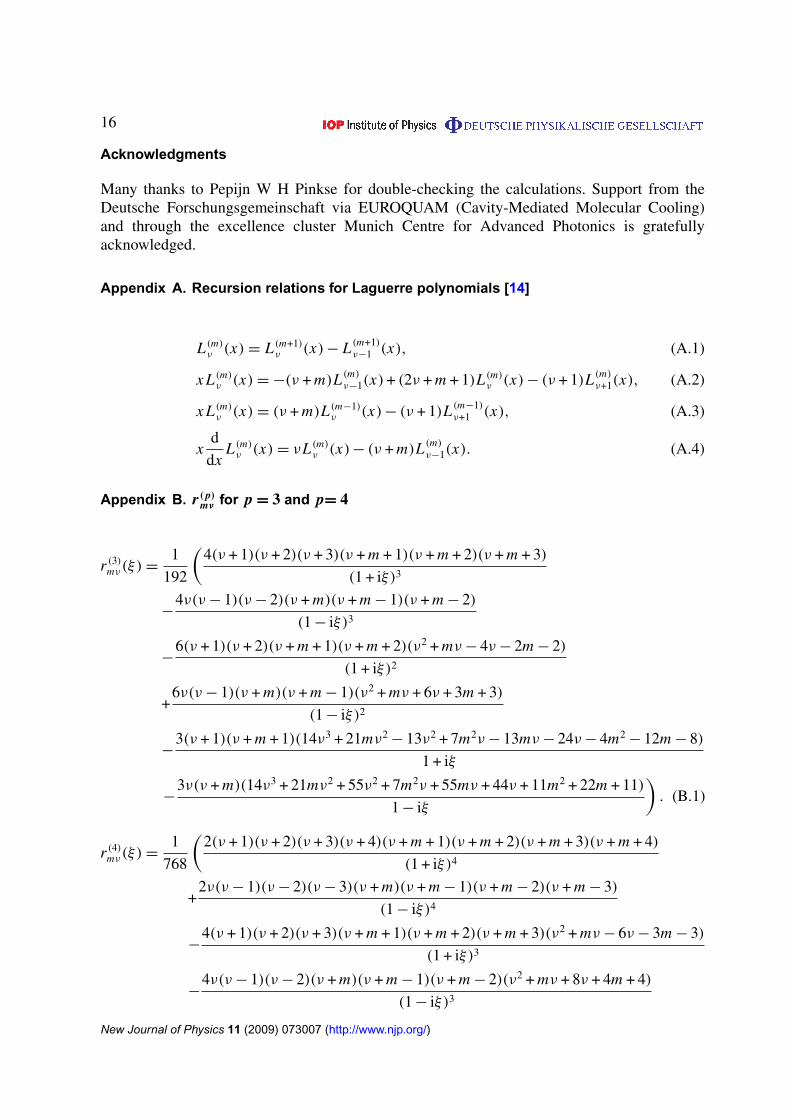
Appendix A. Recursion relations for Laguerre polynomials [14]

L (m)ν (x)= L (m+1)ν (x)− L (m+1)

ν−1 (x), (A.1)

x L (m)ν (x)= −(ν + m)L (m)ν−1(x)+ (2ν + m + 1)L (m)ν (x)− (ν + 1)L (m)ν+1(x), (A.2)

x L (m)ν (x)= (ν + m)L (m−1)ν (x)− (ν + 1)L (m−1)

ν+1 (x), (A.3)

xd

dxL (m)ν (x)= νL (m)ν (x)− (ν + m)L (m)ν−1(x). (A.4)

Appendix B. r ( p)mν for p = 3 and p= 4

r (3)mν (ξ)=1

192

(4(ν + 1)(ν + 2)(ν + 3)(ν + m + 1)(ν + m + 2)(ν + m + 3)

(1 + iξ)3

−4ν(ν− 1)(ν− 2)(ν + m)(ν + m − 1)(ν + m − 2)

(1 − iξ)3

−6(ν + 1)(ν + 2)(ν + m + 1)(ν + m + 2)(ν2 + mν− 4ν− 2m − 2)

(1 + iξ)2

+6ν(ν− 1)(ν + m)(ν + m − 1)(ν2 + mν + 6ν + 3m + 3)

(1 − iξ)2

−3(ν + 1)(ν + m + 1)(14ν3 + 21mν2

− 13ν2 + 7m2ν− 13mν− 24ν− 4m2− 12m − 8)

1 + iξ

−3ν(ν + m)(14ν3 + 21mν2 + 55ν2 + 7m2ν + 55mν + 44ν + 11m2 + 22m + 11)

1 − iξ

). (B.1)

r (4)mν (ξ)=1

768

(2(ν + 1)(ν + 2)(ν + 3)(ν + 4)(ν + m + 1)(ν + m + 2)(ν + m + 3)(ν + m + 4)

(1 + iξ)4

+2ν(ν− 1)(ν− 2)(ν− 3)(ν + m)(ν + m − 1)(ν + m − 2)(ν + m − 3)

(1 − iξ)4

−4(ν + 1)(ν + 2)(ν + 3)(ν + m + 1)(ν + m + 2)(ν + m + 3)(ν2 + mν− 6ν− 3m − 3)

(1 + iξ)3

−4ν(ν− 1)(ν− 2)(ν + m)(ν + m − 1)(ν + m − 2)(ν2 + mν + 8ν + 4m + 4)

(1 − iξ)3

New Journal of Physics 11 (2009) 073007 (http://www.njp.org/)

17

+(ν + 1)(ν + 2)(ν + m + 1)(ν + m + 2)

(1 + iξ)2(ν4 + 2mν3

− 54ν3 + m2ν2− 81mν2 + 111ν2

−27m2ν + 111mν + 180ν + 30m2 + 90m + 60)+ν(ν− 1)(ν + m)(ν + m − 1)

(1 − iξ)2

×(ν4 + 2mν3 + 58ν3 + m2ν2 + 87mν2 + 279ν2 + 29m2ν + 279mν + 208ν + 58m2

+104m + 46)+(ν + 1)(ν + m + 1)

1 + iξ

(ν6 + (3m + 2)ν5 + (3m2 + 5m − 311)ν4

+(m3 + 4m2− 622m + 84)ν3 + (m3

− 382m2 + 126m + 653)ν2

+(−71m3 + 102m2 + 653m + 540)ν + 30m3 + 162m2 + 270m + 138)

+ν(ν + m)

1 − iξ

(ν6+(3m+ 4)ν5+ (3m2+10m−306)ν4+(m3+ 8m2

− 612m−1328)ν3

+(2m3− 376m2

− 1992m − 1470)ν2− (70m3 + 866m2 + 1470m + 734)ν

−(101m3 + 323m2 + 367m + 145))). (B.2)

References

[1] Flammer C 1957 Spheroidal Wave Functions (Palo Alto, CA: Stanford University Press)[2] Meixner J and Andrejewski W 1950 Ann. Phys. 442 157[3] McDonald K T 2003 arXiv:physics/0312024v1[4] Siegman A E 1986 Lasers (Herndon, VA: University Science Books)[5] Agrawal G P and Pattanayak D N 1979 J. Opt. Soc. Am. 69 575[6] Zeppenfeld M, Koch M, Hagemann B, Motsch M, Pinkse P W H and Rempe G in preparation[7] Lax M, Louisell W H and McKnight W B 1975 Phys. Rev. A 11 1365[8] Baber W G and Hassé H R 1935 Proc. Camb. Phil. Soc. 31 564[9] Svartholm N 1938 Z. Phys. 111 186

[10] Meixner J 1944 Ber. Z. W. B., Nr. 1952[11] Flammer C 1953 J. Appl. Phys. 24 1218[12] Sakurai J J 1994 Modern Quantum Mechanics (Reading, MA: Addison Wesley)[13] Pinney E 1946 J. Math. Phys. 25 49[14] Abramowitz M and Stegun I A 1964 Handbook of Mathematical Functions (New York: Dover)[15] Jackson J D 1998 Classical Electrodynamics (New York: Wiley)[16] Lazutkin V F 1968 Opt. Spectra 24 236[17] Laabs H and Friberg A T 1999 IEEE J. Quantum Electron. 35 198[18] Zomer F, Soskov V and Variola A 2007 Appl. Opt. 46 6859

New Journal of Physics 11 (2009) 073007 (http://www.njp.org/)