solution of inverse problem of … · approval of the thesis: solution of inverse problem of...
TRANSCRIPT

SOLUTION OF INVERSE PROBLEM OF ELECTROCARDIOGRAPHY USINGSTATE SPACE MODELS
A THESIS SUBMITTED TOTHE GRADUATE SCHOOL OF NATURAL AND APPLIED SCIENCES
OFMIDDLE EAST TECHNICAL UNIVERSITY
BY
UMIT AYDIN
IN PARTIAL FULFILLMENT OF THE REQUIREMENTSFOR
THE DEGREE OF MASTER OF SCIENCEIN
ELECTRICAL AND ELECTRONICS ENGINEERING
SEPTEMBER 2009
Approval of the thesis:
SOLUTION OF INVERSE PROBLEM OF ELECTROCARDIOGRAPHY USINGSTATE SPACE MODELS
submitted by UMIT AYDIN in partial fulfillment of the requirements for the degreeof Master of Science in Electrical and Electronics Engineering Department, MiddleEast Technical University by, Prof. Dr. Canan OzgenDean, Graduate School of Natural and Applied Sciences
Prof. Dr. Ismet ErkmenHead of Department, Electrical and Electronics Engineering
Assist. Prof. Dr. Yesim Serinagaoglu DogrusozSupervisor, Electrical and Electronics Engineering Dept, METU
Examining Committee Members:
Prof. Dr. Murat EyubogluElectrical and Electronics Engineering, METU
Assist. Prof. Dr. Yesim Serinagaoglu DogrusozElectrical and Electronics Engineering, METU
Prof. Dr. Nevzat Guneri GencerElectrical and Electronics Engineering, METU
Prof. Dr. Kemal LeblebiciogluElectrical and Electronics Engineering, METU
Dr. Ozlem BirgulTUBITAK
Date:

I hereby declare that all information in this document has been obtained andpresented in accordance with academic rules and ethical conduct. I also declarethat, as required by these rules and conduct, I have fully cited and referenced allmaterial and results that are not original to this work.
Name, Last Name: UMIT AYDIN
Signature :
iii

ABSTRACT
SOLUTION OF INVERSE PROBLEM OF ELECTROCARDIOGRAPHY USINGSTATE SPACE MODELS
Aydın, Umit
M.S., Department of Electrical and Electronics Engineering
Supervisor : Assist. Prof. Dr. Yesim Serinagaoglu Dogrusoz
September 2009, 108 pages
Heart is a vital organ that pumps blood to whole body. Synchronous contraction of the
heart muscles assures that the required blood flow is supplied to organs. But some-
times the synchrony between those muscles is distorted, which results in reduced
cardiac output that might lead to severe diseases, and even death. The most com-
mon of heart diseases are myocardial infarction and arrhythmias. The contraction of
heart muscles is controlled by the electrical activity of the heart, therefore determina-
tion of that electrical activity could give us the information regarding the severeness
and type of the disease. In order to diagnose heart diseases, classical 12 lead elec-
trocardiogram (ECG) is the standard clinical tool. Although many cardiac diseases
could be diagnosed with the 12 lead ECG, measurements from sparse electrode lo-
cations limit the interpretations. The main objective of this thesis is to determine
the cardiac electrical activity from dense body surface measurements. This problem
is called the inverse problem of electrocardiography. The high resolution maps of
epicardial potentials could supply the physician the information that could not be ob-
tained with any other method. But the calculation of those epicardial potentials are
iv

not easy; the problem is severely ill-posed due to the discretization and attenuation
within the thorax. To overcome this ill-posedness, the solution should be constrained
using prior information on the epicardial potential distributions. In this thesis, spatial
and spatio-temporal Bayesian maximum a posteriori estimation (MAP), Tikhonov
regularization and Kalman filter and Kalman smoother approaches are used to over-
come the ill-posedness that is associated with the inverse problem of ECG. As part
of the Kalman filter approach, the state transition matrix (STM) that determines the
evolution of epicardial potentials over time is also estimated, both from the true epi-
cardial potentials and previous estimates of the epicardial potentials. An activation
time based approach was developed to overcome the computational complexity of
the STM estimation problem. Another objective of this thesis is to study the effects
of geometric errors to the solutions, and modify the inverse solution algorithms to
minimize these effects. Geometric errors are simulated by changing the size and the
location of the heart in the mathematical torso model. These errors are modeled as
additive Gaussian noise in the inverse problem formulation. Residual-based and ex-
pectation maximization methods are implemented to estimate the measurement and
process noise variances, as well as the geometric noise.
Keywords: Inverse electrocardiography, Spatio-temporal methods, Kalman filter, Noise
estimation, Geometric errors
v

OZ
ELEKTROKARDIYOGRAFIDE GERI PROBLEMIN DURUM UZAYIMODELLERI KULLANILARAK COZUMU
Aydın, Umit
Yuksek Lisans, Elektrik ve Elektronik Muhendisligi Bolumu
Tez Yoneticisi : Yrd. Doc. Dr. Yesim Serinagaoglu Dogrusoz
Eylul 2009, 108 sayfa
Kalp butun vucuda kan pompalayan hayati bir organdır. Kalp kaslarındaki senkron
kasılma ve gevsemeler organlara gerekli kan akısının gerceklesmesini saglamaktadır.
Fakat bazen bu kaslar arasındaki senkronizasyon bozulmakta ve dusen kalp debisi
olume kadar gidebilen hastalıklara sebep olabilmektedir. Bu hastalıklardan en cok
karsılasılanlar enfarktus ve aritmidir. Kalp kaslarındaki kasılmalar elektrik sinyalleri
ile kontrol edilmektedir, bu sebeple kalbin elektriksel aktivitesi hakkında bilgi edin-
mek bize hastalıkların cinsi ve ciddiyeti hakkında da cok onemli bilgiler vermektedir.
Gunumuzde kalp hastalıklarının techisinde kullanılan standart klinik yontem klasik
12 kanallı elektrokardiyografidir (EKG). Bu yontem bircok hastalıgın teshisinde kul-
lanılsa da vucut yuzeyinden alınan olcumlerin seyrekligi cıkarımları sınırlamaktadır.
Bu tezde baslıca amac kalpteki elektriksel aktiviteyi vucut yuzeyinden sık bir cekilde
alınan olcumlerden bulmaktır ve bu ters elektrokardiyografi problemi olarak tanımlan-
maktadır. Elde edilen yuksek cozunurluklu epikart potansiyel haritaları ise dok-
tora backa hicbir girisimsiz yontemle elde edilemeyecek bilgiler verir. Fakat epikart
potansiyellerini hesaplamak kolay degildir cunku, ters EKG problemi gogus kafesinde
vi

sinyallerin ugradıgı ayrıklasma ve zayıflama sebebiyle kotu konumlanmıstır. Bu
problemin ustesinden gelebilmek amacıyla, epikart potansiyel dagılımları ile ilgili
onsel bilgiler kullanılarak cozume bazı kısıtlamalar getirilir. Bu tezde uzamsal ve
zaman-uzamsal Bayes en buyuk sonsal kestrim (MAP), Tikhonov duzenlilestirmesi
ile Kalman filtre ve yumusatıcı bu kotu konumlandırılmıs problemi cozme amaclı
kullanılmıstır. Kalman filtre yaklasımının bir uzantısı olarak epikart potansiyellerinin
zamana baglı degisimini modelleyen durum gecis matrisi (DGM) hem gercek epikart
potansiyellerinden hem de baska yontemlerle kestirilen epikart potansiyellerinden
elde edilmistir. Bu tezin baska bir hedefi ise geometrik hataların cozumlere etki-
lerini incelemek ve ters cozum algoritmalarını bu etkileri minimize edecek sekilde
modifiye etmektir. Bu kapsamda geometrik hatalar kalbin boyut ve pozisyonunun
matematiksel modelde degistirilmesi ile elde edilmistir. Bu hatalar ters problem
formulasyonunda eklenir Gaussian gurultu olarak modellenmislerdir. Daha sonra
ise durum ve olcum gurultu varyansları ile geometrik hatadan kaynaklanan gurultu
varyansı, artıklardan yararlanan algoritma ve beklenti encoklaması kullanılarak kes-
tirilmeye calısılmıstır.
Anahtar Kelimeler: Geri elektrokardiyografi, Uzamsal-zamansal yontemler, Kalman
filtre, Gurultu kestirimi, Geometrik hata
vii

ACKNOWLEDGMENTS
I would like to thank my thesis supervisor Assist. Prof. Dr. Yesim Serinagaoglu
Dogrusoz for providing me this research opportunity and guiding me through the
study.
This study is part of the project 105E070 that is supported by Turkish Scientific and
Technological Research Council (TUBITAK). I thank to Dr. Robert S. MacLeod
from University of Utah, Nora Eccles Harrison CVRTI and the SCI Institute for the
epicardial measurements used in the study and the map3d software.
I would like to thank all my colleagues Dr. Ozlem Birgul, Murat Onal, Ugur Cune-
dioglu, Ceren Bora and Alireza Mazloumi at ECG laboratory for their comments and
technical supports.
I also would like to thank Prof. Dr. Murat Eyuboglu and all my colleagues at MRI
research laboratory Volkan Emre Arpınar, Evren Degirmenci, Gokhan Eker, Rasim
Boyacıoglu, Tankut Topal and Ali Ersoz for their supports.
I also would like to express my appreciation to all my friends especially Sedat Dogru,
Guven Cetinkaya, Kerim Kara, Ozan Ozyurt, Masood Jabarnejad and Ersin Karcı for
their enthusiastic support throughout the development of this thesis.
Finally, I like to express very special thanks to my dear family for their endless sup-
port and love throughout my education.
viii

TABLE OF CONTENTS
ABSTRACT . . . . . . . . . . . . . . . . . . . . . . . . . . . . . . . . . . . . iv
OZ . . . . . . . . . . . . . . . . . . . . . . . . . . . . . . . . . . . . . . . . . vi
ACKNOWLEDGMENTS . . . . . . . . . . . . . . . . . . . . . . . . . . . . . viii
TABLE OF CONTENTS . . . . . . . . . . . . . . . . . . . . . . . . . . . . . ix
LIST OF TABLES . . . . . . . . . . . . . . . . . . . . . . . . . . . . . . . . xii
LIST OF FIGURES . . . . . . . . . . . . . . . . . . . . . . . . . . . . . . . . xiv
CHAPTERS
1 INTRODUCTION . . . . . . . . . . . . . . . . . . . . . . . . . . . 1
1.1 Motivation of the Thesis . . . . . . . . . . . . . . . . . . . . 1
1.2 Contributions of the Thesis . . . . . . . . . . . . . . . . . . 2
1.3 Scope of the Thesis . . . . . . . . . . . . . . . . . . . . . . 3
2 BACKGROUND INFORMATION . . . . . . . . . . . . . . . . . . . 4
2.1 Introduction . . . . . . . . . . . . . . . . . . . . . . . . . . 4
2.2 Anatomy of the Heart . . . . . . . . . . . . . . . . . . . . . 4
2.3 Physiology of the Heart . . . . . . . . . . . . . . . . . . . . 5
2.3.1 Cardiac Conduction System . . . . . . . . . . . . 5
2.3.2 Cardiac Action Potential . . . . . . . . . . . . . . 8
2.3.3 Electrocardiography . . . . . . . . . . . . . . . . 8
2.4 Cardiac Diseases . . . . . . . . . . . . . . . . . . . . . . . . 9
2.4.1 Myocardial Infarction . . . . . . . . . . . . . . . . 9
2.4.2 Cardiac Re-entry Phenomenon . . . . . . . . . . . 13
2.4.3 Ventricular Fibrillation . . . . . . . . . . . . . . . 15
2.4.4 Atrial Fibrillation and Flutter . . . . . . . . . . . . 15
ix
2.5 Forward Problem of Electrocardiography . . . . . . . . . . . 16
2.5.1 Obtaining the Anatomical Information . . . . . . . 16
2.5.2 Numerical Solution Techniques . . . . . . . . . . 17
2.6 Inverse Problem of Electrocardiography . . . . . . . . . . . 18
2.6.1 Cardiac Source Models . . . . . . . . . . . . . . . 19
2.6.1.1 Epicardial and Endocardial PotentialDistributions . . . . . . . . . . . . . . 19
2.6.1.2 Transmembrane Potentials . . . . . . 20
2.6.1.3 Activation Time Imaging . . . . . . . 21
2.6.2 Literature Survey on Inverse Solution Approaches . 22
2.6.2.1 Methods in Literature to Deal with Ill-posedness for Epicardial Potential BasedModel . . . . . . . . . . . . . . . . . 22
2.6.2.2 Other Approaches to Obtain CardiacElectrical Activity . . . . . . . . . . . 26
2.6.3 Validation Studies and Human Experiments . . . . 27
2.6.4 Geometric Errors . . . . . . . . . . . . . . . . . . 28
3 THEORY . . . . . . . . . . . . . . . . . . . . . . . . . . . . . . . . 31
3.1 Problem Definition . . . . . . . . . . . . . . . . . . . . . . . 31
3.2 Inverse Problem Solution Algorithms . . . . . . . . . . . . . 34
3.2.1 Tikhonov Regularization . . . . . . . . . . . . . . 34
3.2.2 Bayesian Maximum A Posteriori Estimation . . . . 36
3.2.3 Temporal Bayesian-MAP . . . . . . . . . . . . . . 37
3.2.4 Kalman Filter and Smoother . . . . . . . . . . . . 38
3.2.5 Determination of STM for Kalman Filter from Epi-cardial Potentials . . . . . . . . . . . . . . . . . . 41
3.3 Enhanced Noise Model for Geometric Error Compensation . 43
3.4 System Identification Problem . . . . . . . . . . . . . . . . . 45
3.4.1 Determination of Measurement and Process NoiseCovariance Matrices Using Residuals . . . . . . . 45
3.4.2 Determination of Measurement and Process NoiseCovariances Using Expectation Maximization . . . 46
x

4 RESULTS AND DISCUSSION . . . . . . . . . . . . . . . . . . . . 48
4.1 Simulated Data . . . . . . . . . . . . . . . . . . . . . . . . . 48
4.2 Validation Methods . . . . . . . . . . . . . . . . . . . . . . 49
4.3 Reduction of the Problem Size for Inverse ECG Solution Us-ing Kalman Filter . . . . . . . . . . . . . . . . . . . . . . . 51
4.3.1 Comparison of the Reduced Formulation for STMCalculation with the Original One for 64 Node Data 51
4.3.2 Comparison of the Proposed Problem DimensionReduction Techniques for STM Calculation with490 Node Data . . . . . . . . . . . . . . . . . . . 56
4.4 Studies on the Calculation of State Transition Matrix withoutUsing Real Epicardial Potentials . . . . . . . . . . . . . . . 62
4.5 The Effects of Geometric Error in Cardiac Electrical Imag-ing and A Statistical Model to Overcome Those Errors: En-hanced Noise Model . . . . . . . . . . . . . . . . . . . . . . 72
4.5.1 Effects of Geometric Errors . . . . . . . . . . . . . 73
4.5.2 Enhanced Noise Model to Compensate GeometricErrors . . . . . . . . . . . . . . . . . . . . . . . . 76
4.6 Determination of the Measurement and Process Noise Co-variance Matrices Using Residuals . . . . . . . . . . . . . . 81
4.7 Expectation Maximization Algorithm to Determine Measure-ment and Process Noise Covariance Matrices . . . . . . . . . 85
5 CONCLUSIONS . . . . . . . . . . . . . . . . . . . . . . . . . . . . 95
5.1 Spatio-temporal Methods for Inverse Problem of ECG . . . . 96
5.2 The Effects of Geometrics Errors to the Solution of InverseECG Problem . . . . . . . . . . . . . . . . . . . . . . . . . 97
5.3 Estimation of the Measurement and Process Noise Covari-ance Matrices from Body Surface Potentials . . . . . . . . . 98
5.4 Future Works . . . . . . . . . . . . . . . . . . . . . . . . . . 100
REFERENCES . . . . . . . . . . . . . . . . . . . . . . . . . . . . . . . . . . 101
xi

LIST OF TABLES
TABLES
Table 2.1 The reasons for cardiac re-entry mechanism and possible diseases
causing those. . . . . . . . . . . . . . . . . . . . . . . . . . . . . . . . . 15
Table 4.1 Means and standard deviations of CC and RDMS values, average
related node numbers and the time consumptions of different scenarios to
reduce the problem dimension of STM calculation for 64 node case. . . . . 53
Table 4.2 Means and standard deviations of CC and RDMS values, average
related node numbers and the time consumptions of different scenarios to
reduce the problem dimension of STM calculation for 490 node case. . . . 58
Table 4.3 Means and standard deviations of CC and RDMS values for spatial
and spatio-temporal methods. . . . . . . . . . . . . . . . . . . . . . . . . 67
Table 4.4 The CC and RDMS values for wrong determination of heart’s size. . 75
Table 4.5 The CC and RDMS values for the wrong determination of the heart’s
location. . . . . . . . . . . . . . . . . . . . . . . . . . . . . . . . . . . . 75
Table 4.6 The CC and RDMS values when enhanced noise model is used. . . . 77
Table 4.7 CC and RDMS values for Kalman-Real and Kalman-Bayes when
noise covariances are calculated from residuals. . . . . . . . . . . . . . . 82
Table 4.8 CC and RDMS values for Kalman-Real and Kalman-Bayes when
noise covariances are calculated from residuals with geometric errors are
present(15mm shift in heart’s position and 0.95 change in heart’s size). . . 82
Table 4.9 CC and RDMS values for Kalman-Real and Kalman-Bayes when
only measurement noise covariances is calculated from residuals. . . . . . 83
xii

Table 4.10 CC and RDMS values for Kalman-Real and Kalman-Bayes when
only measurement noise covariance is calculated from residuals with ge-
ometric errors are present(15mm shift in heart’s position and 0.95 change
in heart’s size). . . . . . . . . . . . . . . . . . . . . . . . . . . . . . . . . 84
xiii
LIST OF FIGURES
FIGURES
Figure 2.1 Layers of the heart. . . . . . . . . . . . . . . . . . . . . . . . . . . 6
Figure 2.2 Anatomy of the heart. . . . . . . . . . . . . . . . . . . . . . . . . 7
Figure 2.3 The action potential waveforms for different cardiac tissues. . . . . 9
Figure 2.4 Action potential wavefront and ion permeabilities for a ventricular
muscle cell. . . . . . . . . . . . . . . . . . . . . . . . . . . . . . . . . . 10
Figure 2.5 The path of cardiac impulse conduction and the corresponding re-
gions at the electrocardiogram with the conduction velocities, conduction
times and self-excitatory(intrinsic) frequencies. . . . . . . . . . . . . . . . 11
Figure 2.6 A typical ECG measurement. . . . . . . . . . . . . . . . . . . . . 12
Figure 2.7 The mechanism of cardiac re-entry: At the upper part of the figure
conduction in normal tissue is shown and at at the lower part the re-entry
mechanism is shown. . . . . . . . . . . . . . . . . . . . . . . . . . . . . 14
Figure 2.8 The cardiac re-entry model. . . . . . . . . . . . . . . . . . . . . . 14
Figure 2.9 The movement of depolarization wavefront for atrial flutter and
fibrillation. . . . . . . . . . . . . . . . . . . . . . . . . . . . . . . . . . . 16
Figure 3.1 The plot of eigenvalues of a homogeneous transfer matrix obtained
with BEM . . . . . . . . . . . . . . . . . . . . . . . . . . . . . . . . . . 33
Figure 3.2 An example L-Curve plot for inverse ECG problem . . . . . . . . . 35
Figure 4.1 Schematic representation of the forward problem. . . . . . . . . . . 49
Figure 4.2 Sample epicardial and body surface potential potential maps plot-
ted with map3d for a certain time instant. . . . . . . . . . . . . . . . . . . 51
xiv
Figure 4.3 The nodes that are related to 230’th node for STM calculation for
different scenarios for the case of 490 epicardial nodes. . . . . . . . . . . 53
Figure 4.4 Schematic representation of the simulation procedure. . . . . . . . 54
Figure 4.5 Starchart representation of time consumption, CC and RDMS. . . . 55
Figure 4.6 Epicardial potential map for 64 node solution with 37 ms after the
first stimulus. . . . . . . . . . . . . . . . . . . . . . . . . . . . . . . . . . 57
Figure 4.7 Starchart representation of time consumption, CC and RDMS. . . . 59
Figure 4.8 Epicardial potential map for 490 node solution at 57 ms after the
first stimulus. . . . . . . . . . . . . . . . . . . . . . . . . . . . . . . . . . 61
Figure 4.9 Schematic representation of the simulation procedure for Bayes-
Train, Tikhonov, Kalman-Bayes, Kalman-Tikh and Kalman-Direct ap-
proaches . . . . . . . . . . . . . . . . . . . . . . . . . . . . . . . . . . . 65
Figure 4.10 Starchart representation of time consumption, CC and RDMS. . . . 66
Figure 4.11 Epicardial potential map for different STM solutions at 45 ms after
the first stimulus. . . . . . . . . . . . . . . . . . . . . . . . . . . . . . . . 69
Figure 4.12 The CC and RDMS values of different STM solutions with respect
to time. . . . . . . . . . . . . . . . . . . . . . . . . . . . . . . . . . . . . 70
Figure 4.13 The real and estimated potential signal plot for the 365’th node on
epicardium . . . . . . . . . . . . . . . . . . . . . . . . . . . . . . . . . . 71
Figure 4.14 The schematic representation of the simulation procedure to study
geometric errors. . . . . . . . . . . . . . . . . . . . . . . . . . . . . . . . 74
Figure 4.15 The change in RDMS values for different values of Enhanced noise
model with geometric errors present for Bayesian-MAP. . . . . . . . . . . 77
Figure 4.16 The change in RDMS values for different values of Enhanced noise
model with geometric errors present for Kalman filter. . . . . . . . . . . . 78
Figure 4.17 The comparison of epicardial potential maps for scale 0.95 that do
and do not use enhanced noise model. . . . . . . . . . . . . . . . . . . . . 79
Figure 4.18 The comparison of epicardial potential maps for 15 mm shift that
do and do not use enhanced noise model. . . . . . . . . . . . . . . . . . . 80
xv

Figure 4.19 Epicardial potential maps for 54 ms after the first stimulus. The
map solutions of both Kalman-Real and Kalman-Bayes are given when
15 mm shift geometric error is present. . . . . . . . . . . . . . . . . . . . 85
Figure 4.20 The evolution of RDMS values with respect to iterations of the EM
algorithm for Kalman-Real and Kalman-Bayes techniques for 15 and 30
dB Gaussian noise. . . . . . . . . . . . . . . . . . . . . . . . . . . . . . . 87
Figure 4.21 The evolution of RDMS values with respect to iterations of the EM
algorithm which updates only measurement noise covariance for Kalman-
Real and Kalman-Bayes techniques for 10 and 15 mm shift and 0.90 and
0.95 scale geometric errors. . . . . . . . . . . . . . . . . . . . . . . . . . 89
Figure 4.22 The evolution of RDMS values with respect to iterations of the
EM algorithm for Kalman-Real and Kalman-Bayes techniques for 15 mm
shift and 0.95 scale geometric errors. . . . . . . . . . . . . . . . . . . . . 90
Figure 4.23 Epicardial potential maps for 39 ms after the first stimulus. The
map solutions of both Kalman-Real and Kalman-Bayes are given when
15 dB Gaussian noise is added to the system. . . . . . . . . . . . . . . . . 92
Figure 4.24 Epicardial potential maps for 39 ms after the first stimulus. The
map solutions of both Kalman-Real and Kalman-Bayes are given when
15 mm shift geometric error is present. . . . . . . . . . . . . . . . . . . . 93
Figure 4.25 Epicardial potential maps for 39 ms after the first stimulus. The
map solutions of both Kalman-Real and Kalman-Bayes are given when
0.95 scale geometric error is present. . . . . . . . . . . . . . . . . . . . . 94
xvi
CHAPTER 1
INTRODUCTION
1.1 Motivation of the Thesis
Heart failure affects approximately 15 million people worldwide and since 1968, the
role of heart failure as the primary cause of death has increased fourfold [1]. Only in
European Union over 1.9 million deaths annually are due to cardiac diseases. Ar-
rhythmias are among the major causes of heart failure. In order to diagnose ar-
rhythmias, knowledge about the electrical activity within the heart is vital. Classi-
cal 12-lead electrocardiogram (ECG) is the standard diagnostic tool to measure the
electrical activity of the heart. However, although physicians could diagnose certain
pathologies with the 12-lead ECG, this technique’s low resolution limits its benefits
significantly; for example, precise localization of pathologies like myocardial infarcts
and arrhythmogenic foci is not possible with the 12-lead ECG [2]. Furthermore, the
12-lead ECG could only diagnose %60 of acute inferior myocardial infarctions [3].
The 12-lead ECG also suffers from the effects of inhomogeneity within the thorax,
and Brody and respiration effects, which cause wrong interpretations [4]. For clinical
purposes, catheters are used to obtain details about the heart’s electrical activity [5].
High resolution images are obtained with these catheters; however, the invasive na-
ture of this technique restricts its usage. There are also other non-invasive techniques
to monitor cardiac behavior such as cardiac CT, nuclear imaging, stress electrocardio-
graphy and echocardiography. Inverse problem of ECG, which is a method to provide
high resolution images of the heart’s electrical activity, could support the diagnosis
made based on the 12-lead ECG. In the inverse ECG problem high resolution cardiac
electrical activity is estimated noninvasively from dense body surface potential mea-
1

surements (usually minimum 64 electrodes). Some advantages of using this type of
electrocardiographic imaging are [6]:
• To screen people that have higher risks for arrhythmias.
• To find the source of patient specific arrhythmia mechanism to determine the
best cure.
• To determine the optimal location and size of the diseased tissue for ablation
and targeted drug delivery.
• To assess the success of the therapy over time.
• To further study the mechanism and properties of arrhythmias.
Due to above cited reasons and benefits, the studies on electrocardiographic imaging
continues faster than ever before. The main motivation of this thesis is to make a
contribution to those efforts.
1.2 Contributions of the Thesis
• The performances of spatio-temporal methods for the solution of inverse prob-
lem of electrocardiography are compared.
• New techniques to determine the state transition matrix (STM), which tempo-
rally maps the epicardial potentials with each other, are employed to solve the
inverse problem of ECG using the Kalman filter and smoother. Those tech-
niques include reduction of the problem size for faster computation using an
activation time based approach and the calculation of the STM from previ-
ous estimates such as Bayesian maximum a posteriori estimation (MAP) and
Tikhonov regularization instead of from real epicardial potentials.
• The effects of geometric errors to Bayesian MAP and Kalman filter solutions
are studied.
• A statistical noise model that also includes the effects of geometric errors is
modified to be used in the inverse problem of ECG.
2

• A residual based method and a method based on expectation- maximization
(EM) algorithm are used to estimate the noise covariances needed in the Bayesian
MAP estimation and the Kalman filter algorithms. The two proposed noise es-
timation methods are used to estimate the measurement and process noise co-
variances in the Kalman filter approach, with or without additional geometric
noise.
1.3 Scope of the Thesis
In this thesis the second chapter is devoted to the background information. In this
chapter, first anatomy and physiology of the heart is given. Then most common
cardiac diseases are explained with a stress on arrhythmias. Next, the forward and
inverse problems of ECG are defined along with a literature survey on these topics.
Finally, the chapter is concluded with a short section on validation of the inverse ECG
problem solutions and studies on human subjects.
The third chapter contains problem definition, theory and methods of the inverse
problem of ECG in terms of epicardial potentials. In this chapter after the problem
definition is given, the second part includes a detailed explanation of Tikhonov reg-
ularization, spatial and spatio-temporal Bayesian MAP estimation, Kalman filter and
smoother and the estimation of STM. Then a statistical model used to overcome the
effects of the geometric errors is explained. The final part of this chapter is devoted
to the noise estimation algorithms.
In the fourth chapter, the application details of the algorithms given in theory section
are provided, along with the results and the discussions of those results.
At the last chapter, conclusions of this study are given.
3
CHAPTER 2
BACKGROUND INFORMATION
2.1 Introduction
In this chapter first anatomy and physiology of the heart is explained shortly. Then a
brief information is given about main cardiac diseases with the focus on arrhythmias.
Then recent progresses on the forward and inverse problem of electrocardiography
is given. The forward problem of ECG targets the determination of body surface
potentials from cardiac electrical activity, and the inverse problem of electrocardiog-
raphy, which is the main topic of this thesis, is defined as the determination of cardiac
electrical activity from body surface potentials.
2.2 Anatomy of the Heart
The human heart is located in the middle mediastinum of the thorax and weights
around 250-300 g. It is a muscular organ that is enclosed with the pericardium. There
is a small region between the fibrous sac pericardium and the heart which is filled with
a fluid and this fluid serves as a lubricant agent for heart that helps avoiding problems
that could occur during movement due to contractions [7]. If we omit pericardium,
heart is composed of three layers as seen in Figure 2.1. Those layers are:
• Epicardium: This is the outer layer of the heart and surrounded by peri-
cardium. The potentials on epicardium (epicardial potentials) are widely used
as cardiac sources in inverse and forward problems of electrocardiography.
4

• Myocardium: This layer is in between epicardium and endocardium. This is
the thickest layer and it contains the myocytes (striated muscle cells) whose
synchronous contraction and relaxation results in pumping of the blood. The
main objective in electrocardiographic imaging is the determination of the ac-
tivity within this region. The solutions in terms of epicardial or endocardial
potentials are obtained due to their close location to myocardium.
• Endocardium: This is the inner layer of the heart and it has a smooth surface to
allow blood flow with minimum resistance. The endocardial potentials which
can be recorded with catheters are also used as cardiac sources for electrocar-
diographic imaging.
The heart has four chambers as seen in Figure 2.2. The upper ones are the right and
left atrium which are responsible for collecting blood from vessels. The lower ones
are called right and left ventricle. The right ventricle pumps the blood to lungs and the
left ventricle pumps the blood to body. Because pumping the blood to body requires
more pressure than pumping it to lungs the left ventricle has a thicker myocardial
layer.
2.3 Physiology of the Heart
Heart is an organ that receives the low pressure blood from venous blood vessels and
then ejects it to arterial blood vessels after increasing its pressure. By this way the
nutrients and oxygen needed is supplied to every living cell in human body via blood.
2.3.1 Cardiac Conduction System
For a normal heart, the excitation starts at the sinoatrial (SA) node then spreads to
the atrioventricular (AV) node thorough myocytes at atrium. The only conductive
region between atria and ventricles is the AV node so the depolarization wavefront
spreads through AV node to ventricles. AV node decreases the conduction velocity
and the wavefront spreads through bundle of His to right and left bundle branches
5
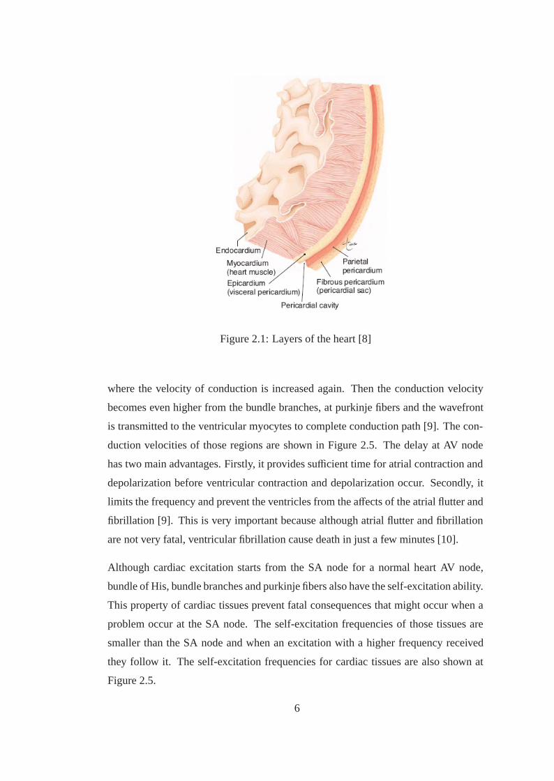
Figure 2.1: Layers of the heart [8]
where the velocity of conduction is increased again. Then the conduction velocity
becomes even higher from the bundle branches, at purkinje fibers and the wavefront
is transmitted to the ventricular myocytes to complete conduction path [9]. The con-
duction velocities of those regions are shown in Figure 2.5. The delay at AV node
has two main advantages. Firstly, it provides sufficient time for atrial contraction and
depolarization before ventricular contraction and depolarization occur. Secondly, it
limits the frequency and prevent the ventricles from the affects of the atrial flutter and
fibrillation [9]. This is very important because although atrial flutter and fibrillation
are not very fatal, ventricular fibrillation cause death in just a few minutes [10].
Although cardiac excitation starts from the SA node for a normal heart AV node,
bundle of His, bundle branches and purkinje fibers also have the self-excitation ability.
This property of cardiac tissues prevent fatal consequences that might occur when a
problem occur at the SA node. The self-excitation frequencies of those tissues are
smaller than the SA node and when an excitation with a higher frequency received
they follow it. The self-excitation frequencies for cardiac tissues are also shown at
Figure 2.5.
6

Figure 2.2: Anatomy of the heart. RA, right atrium; LA, left atrium; RV, right ven-tricle; LV, left ventricle; SVC, superior vena cava; IVC, inferior vena cava; PA, pul-monary artery; PV, pulmonary veins [9].
7

2.3.2 Cardiac Action Potential
Although the action potential wavefront changes for different tissues as seen in Figure
2.3, the generation of the typical cardiac action potential after the stimulus can be
explained with steps below:
1. The quick Na+ channels are opened which causes sodium to flow inward thus
increasing the membrane potential through positive. Then depolarization occur
around +20 mV.
2. Slower K+ channels are opened and the outward flow of K+ stops the rising
potential due to Na+.
3. Na+ channels start closing while K+ channels are still open.
4. Slow Ca++ channels are opened and stay opened for approximately 20 millisec-
ond which causes the plateau in membrane potential potential due to the inward
Ca++ flow.
5. Ca++ channels are closed and repolarization occur with membrane voltage around
-90 mV.
The shape of cardiac action potential differs from the action potential of other ex-
citable tissues in the body. The difference is the plateau present after depolarization
in cardiac action potential. The main reason for this plateau is the 4’th step explained
above so Ca++ channels. This plateau does not occur in other excitable cells because
they do not have Ca++ channels [7]. A typical action potential for a ventricular muscle
cell and the ion permeabilities are shown in Figure 2.4.
2.3.3 Electrocardiography
In electrocardiography (ECG) the summation of cardiac action potentials are mea-
sured. In Figure 2.6 a classical ECG measurement is shown. In this figure [4];
• P represents the atrial depolarization
8

Figure 2.3: The action potential waveforms for different cardiac tissues [11].
• QRS interval represents the ventricular depolarization (also atrial repolarization
occur at this interval but it is surpassed by ventricular depolarization)
• T represents the ventricular repolarization
2.4 Cardiac Diseases
At this section only some of the cardiac diseases will be explained. The focus will be
on diseases that can be diagnosed with inverse electrocardiography.
2.4.1 Myocardial Infarction
Myocardial infarction is one of the major health problems and each year more than
1.5 million people suffer from it only in United States [7]. Heart muscles are in a con-
tinuous cycle and this process requires energy. The oxygen and nutrients required for
energy production are supplied by coronary arteries. Those arteries might suffer from
occlusions which results in reduced blood flow. This phenomenon is called ischemia.
9
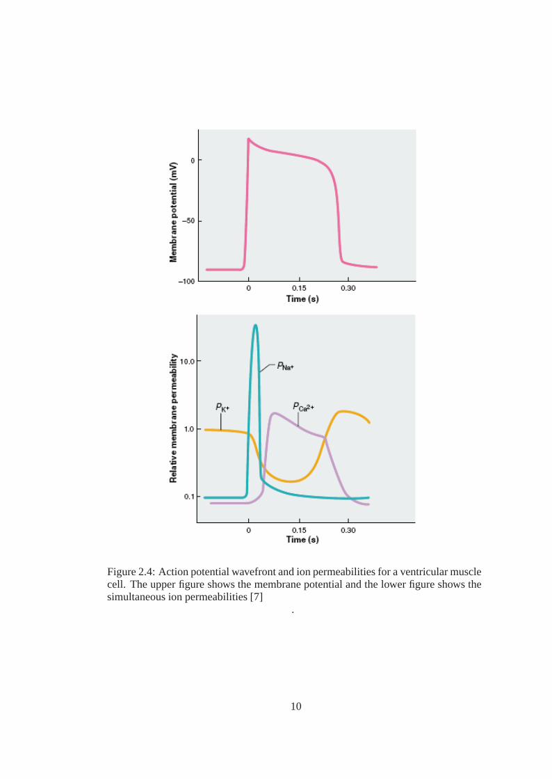
Figure 2.4: Action potential wavefront and ion permeabilities for a ventricular musclecell. The upper figure shows the membrane potential and the lower figure shows thesimultaneous ion permeabilities [7]
.
10

Figure 2.5: The path of cardiac impulse conduction and the corresponding regionsat the electrocardiogram with the conduction velocities, conduction times and self-excitatory (intrinsic) frequencies [11].
11
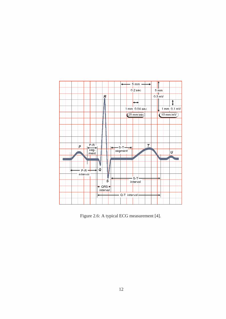
Figure 2.6: A typical ECG measurement [4].
12
If the damage due to ischemia is severe the tissues at that part of the heart might die
and this is called myocardial infarction. Those ischemic regions or infarctions cause
the extracellular conductivity changes which could be detected with investigation of
epicardial potentials [12].
2.4.2 Cardiac Re-entry Phenomenon
In normal circumstances the excitation wavefront follows a predetermined path be-
cause all other paths are obstructed with tissues in refractory period. But sometimes
due to certain problems the wavefront can find other ways to spread and after a period
it comes back and simulates the same tissues again and again unless the conduction
is resynchronized with electroshock.
The causes and mechanism of cardiac re-entry are usually described with cardiac
muscle strips that are cut in a circular shape. Here this convention will be followed
too [10].
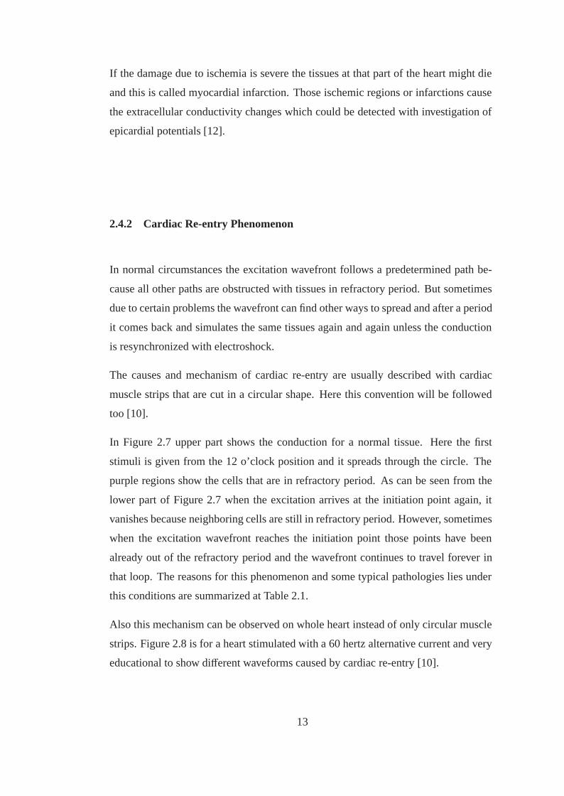
In Figure 2.7 upper part shows the conduction for a normal tissue. Here the first
stimuli is given from the 12 o’clock position and it spreads through the circle. The
purple regions show the cells that are in refractory period. As can be seen from the
lower part of Figure 2.7 when the excitation arrives at the initiation point again, it
vanishes because neighboring cells are still in refractory period. However, sometimes
when the excitation wavefront reaches the initiation point those points have been
already out of the refractory period and the wavefront continues to travel forever in
that loop. The reasons for this phenomenon and some typical pathologies lies under
this conditions are summarized at Table 2.1.
Also this mechanism can be observed on whole heart instead of only circular muscle
strips. Figure 2.8 is for a heart stimulated with a 60 hertz alternative current and very
educational to show different waveforms caused by cardiac re-entry [10].
13

Figure 2.7: The mechanism of cardiac re-entry: At the upper part of the figure con-duction in normal tissue is shown and at at the lower part the re-entry mechanism isshown. [10]
Figure 2.8: The cardiac re-entry model: At the left the initiation of the fibrillation canbe seen with darker pink regions shows the regions in refractory period. The figureon the right hand side shows the propagation paths of those impulses. [10]
14

Table 2.1: The reasons for cardiac re-entry mechanism and possible diseases causingthose.
Cause Possible underlying diseasesThe pathway around the circle is too long Dilated Heart
Blockage of the Purkinje FibersThe velocity of the conduction is too low Ischemia of the muscle
High blood potassium
The refractory period of the muscle Due to some drugs (epinephrine etc.)decreased significantly Repetitive electrical stimulation
2.4.3 Ventricular Fibrillation
Ventricular fibrillation is the most serious cardiac arrythmia and it can cause death if
not treated within 1 to 3 minutes. As explained previously normally the excitation
wavefront follows the same path in every cardiac cycle. But sometimes this path is
distorted and the excitation wavefront follows other paths and returns to itself again
which distorts the synchrony of the heart muscles. Due to this asynchrony sufficient
blood can not be pumped to body which results in unconsciousness in a few seconds
and death in a few minutes [10]. The main reason for ventricular fibrillation is known
as re-entry phenomenon.
2.4.4 Atrial Fibrillation and Flutter
Atrial fibrillation and flutter are problems due to cardiac arrhythmias. The main cause
of those problems is re-entry mechanism. In atrial flutter the depolarization wavefront
spreads in one direction along atria with a much higher frequency than normal (200
to 350 beats per minute). On the other hand in atrial fibrillation there is not a single
depolarization wavefront instead many different wavefronts spread through atria. The
wavefront propagations for those two diseases can be seen at Figure 2.9. Both atrial
flutter and fibrillation cause serious reduction in pumping mechanism of the atria but
those diseases are not as serious as ventricular fibrillation [10].
15

Figure 2.9: The movement of depolarization wavefront for atrial flutter and fibrillation[10].
2.5 Forward Problem of Electrocardiography
The goal in forward problem of ECG is to calculate the body surface potentials from
the cardiac electrical activity. Although it may not seem so meaningful in clinical
sense it has several implementations like [13]:
• Simulation of ECG with computer heart models
• Solution of reciprocal problem of determining currents on heart due to the cur-
rent sources on body surface.
To solve the forward problem of ECG along with the anatomical information also a
numerical solver is required.
2.5.1 Obtaining the Anatomical Information
In order to solve forward or inverse problem of electrocardiography, information
about the geometries (or anatomies) of the organs is a crucial requirement. In the liter-
ature the geometry information is usually obtained by Magnetic Resonance Imaging
(MRI) or Computed Tomography (CT) [2]. The most important criticization about
using those imaging modalities for electrocardiographic imaging is that they are ex-
pensive. Another drawback about those are that they are too heavy and not mobilized
so they can not be used for a system that could overcome the classical 12 lead ECG. In
order to address these problems studies on obtaining necessary geometrical informa-
16

tion for electrocardiographic imaging using other imaging techniques emerge. One
group studies on using electrical impedance tomography (EIT) for this purpose and
try to benefit from its relative cheap price and high mobility [14, 15, 16]. Another
advantage of using EIT is its ability to measure conductivity values of the tissues. By
using these data instead of using predetermined values for each tissue, conductivities
that are specific for each patient could be used to obtain better results. There are also
studies that use three dimensional ultrasound for this purpose [17, 18].
2.5.2 Numerical Solution Techniques
After the geometry information is obtained using imaging modalities described sec-
tion 2.5.1, a numerical approach is needed to calculate the transfer matrix that maps
the parameters of the cardiac sources to body surface potentials. Those numerical
solvers can be categorized as [13]:
• Volume Element Methods:
– Finite Element Method (FEM)
– Finite Difference Method
– Finite Volume Method
• Surface Element Methods:
– Boundary Element Method (BEM)
Here FEM and BEM are compared because the most widely used methods in elec-
trocardiographic imaging are those two. The main advantages and disadvantages of
these methods compared to each other are [13, 19]:
• For FEM solution, whole tissue volume should be discretized, on the other hand
for BEM, only the boundaries of the tissues with different conductivities should
be discretized which reduces the complexity by a great amount.
• FEM could model tissues with anisotropic conductivities such as the the fiber
orientation of the heart. BEM could model only isotropic tissues because only
17
the boundaries of those tissues are discretized. The anisotropies are included
to the BEM model by determining an average of the conductivities that are
longitudinal and transversal to the fiber direction.
• The matrices in FEM method are symmetric, positive definite and sparse but for
BEM those matrices are dense which results in higher memory requirement.
The adaptive methods can be used to refine FEM in order to obtain finer solutions
on the regions where fine solution is needed and coarse solution in regions where the
solutions resolution is not that significant. By this way the extra work to construct
fine meshes everywhere is avoided and this reduces the computation costs [20].
The accuracy of the BEM method is shown to be increased without upsurges in com-
putational complexity using adaptive BEM [21]. For that purpose a coarse initial
mesh is chosen and finer meshes are build using h-adaptive BEM in the literature
[21]. The size of the meshes differ for different locations of the torso model based on
the residual error. This means finer meshes are built for the parts of the torso where
body surface potentials changes more. In that study it is shown that the accuracy can
be increased as much as 10 percent with h-adaptive BEM.
Also there is a study to obtain numerical solution using method of fundamental solu-
tions which eliminates the need to construct meshes [22]. At this technique first an
auxiliary domain which encloses the real domain is constructed with auxiliary bound-
aries. The virtual source points (fundamental solutions) on those auxiliary boundaries
achieves an approximate solution with linear superposition. Then the required epicar-
dial surface potentials are calculated easily because the epicardial boundary is also in
that auxiliary domain. Another advantage of the method of fundamental solutions
over BEM is that the complex singular integrals are avoided [22].
2.6 Inverse Problem of Electrocardiography
The inverse problem of ECG is more meaningful in the clinical sense because from
the measured body surface potentials the unknown cardiac electrical activity is tried to
be calculated. In this section first different types of cardiac sources used to represent
18

the electrical activity are explained. Then a literature survey on the inverse solution
algorithms is given. In the next subsection validation studies and human experiments
are explained. Finally the section is ended with a subsection on geometric errors.
2.6.1 Cardiac Source Models
There are many different cardiac source models that are used in inverse problem of
electrocardiography. The first attempts focus on representing the electrical activity
by one dipole [23]. Then more than one dipole and multipoles are used [24, 13]. The
most frequently used source models today are epicardial or endocardial potential,
transmembrame potential and activation time based models. Thus those techniques
will be explained at this section. All of those techniques have advantages over others
in terms of uniqueness, linearity and the severity of ill-posedness.
• Uniqueness One of the main difficulties about inverse electrocardiography prob-
lem is the non-uniqueness of the problem. Different cardiac source distribu-
tions may result in same body surface potentials which results in physologi-
cally meaningless solutions. In order to overcome this problem physiological
constraints can be used.
• Ill-Posedness Ill-posedness is defined as the phenomenon that even small per-
turbations results in very severe errors in solutions. To overcome this problem
regularization or statistical methods are widely used.
We have used the epicardial based method in our studies due to its advantages that
will be explained shortly.
2.6.1.1 Epicardial and Endocardial Potential Distributions
One widely used model for cardiac sources is in terms of epicardial or endocardial
potentials. Those solutions can be also called as surface potential based models.
Although the cardiac sources are located at myocardium they could also be inter-
preted when potential distribution on surface is obtained. The detailed formulation
19

and information regarding the epicardial potential based model is given at section
3.1. The advantages of formulating the problem in terms of surface potentials are:
[2, 25, 13, 26]:
• In theory because the location of cardiac sources are restricted to the epicardial
or endocardial surface the problem becomes unique.
• The solutions can be verified with either catheter measurements (for endocar-
dial potential map) or sock electrodes (for epicardial potential map). Here we
neglect the effects of surrounding impedances to those potentials which could
change the measurements for example in open heart surgery.
• Another advantage of using epicardial potential based methods is that errors due
to blood masses within the heart are avoided. Those blood masses cause sig-
nificant errors due to the changes in flow and amount. The epicardial potentials
are outside those masses. Thus while the epicardial potentials are calculated
from body surface potentials those blood masses has no effects on solutions.
• The problem can be formulated linearly.
Some groups prefer studying on other formulations due to the disadvantages of sur-
face potential based models such as:
• The problem is highly ill-posed due to the discretization and smoothing effects
on potential signals passing through thorax. To overcome this problem reg-
ularization, statistical methods or filters are used which are explained in the
subsection 2.6.2.1.
• Some studies show that it is affected more from geometric errors compared to
activation time models [27, 28].
2.6.1.2 Transmembrane Potentials
The transmembrane potential (TMP) is the potential difference between inside and
outside of the cell membrane. The calculation of transmembrane potentials at the
myocardium becomes a widely studied model due to advantages such as [29, 30]:
20
• The problem can be formulated as a linear problem.
• Most of the diseases can be diagnosed with studying TMP’s shape and distri-
bution. Epicardial potentials and activation times could easily be obtained from
the TMP distributions.
But it has a very serious limitation, the solution is non-unique so the obtained solution
may not be physiologically meaningful unless additional constraints are used [29].
Also the increase in problem size a major disadvantage.
2.6.1.3 Activation Time Imaging
Although epicardial or endocardial potentials could give significant information re-
garding the myocardium, some groups prefer calculating the myocardial activation
directly from BSP’s. When uniform and isotropic conductivities are assumed along
with zero phase amplitude, the formulation for activation time based model is:
Φ(y, t) =∫
SA(x, y)H(t − τ(x))dS x (2.1)
where H is the Heaviside step function, τ(x) is the activation time of myocardium at
position x, A(x, y) is the uniform double layer transfer function and Φ(y, t) is the body
surface potential at position y. The advantages of this formulation are [2, 25, 13, 26]:
• It deals directly with the phenomenon sought which is the activation times at
myocardium.
• It is better-posed then surface potential methods.
• It deals with only a few parameters eg. the activation time of the tissue at a cer-
tain location whereas the surface potential methods tries to find the potentials
for each time instant which requires a lot more parameters.
• Some studies show that it is affected less from geometric errors comparison
with surface potential based methods [27, 28].
There are also disadvantages of this model:
21

• The solutions cannot be verified directly with measurements as in the case of
surface potential methods.
• The problem is non-linear which results in more complex calculations.
• The model forces the solution of activation times for all tissues based on a
template function that mimics the transmembrane potentials and because this
template function is not valid at ischemic or infarcted regions, the solution fails
[29].
• The isotropy assumption for myocardium limits its results (There are some re-
cent studies that does not require isotropy assumption to overcome this limita-
tion [31]).
2.6.2 Literature Survey on Inverse Solution Approaches
At this subsection first, a literature survey on the solution of inverse problem of ECG
in terms of epicardial potentials and other source models is given then the literature
survey is concluded with some recent works on human studies and validation meth-
ods.
2.6.2.1 Methods in Literature to Deal with Ill-posedness for Epicardial Poten-
tial Based Model
In inverse electrocardiography literature many different techniques were used to solve
inverse problem of electrocardiography. Some of those are:
• Tikhonov Regularization: It is the most widely used method in the literature
and it is explained in detail in section 3.2.1 [32, 33]. Shortly its solution is the
minimization of the sum of the data misfit and a constraint to regularize the
solution.
• Twomey Regularization: It is very similar to Tikhonov regularization but the
constraint is the two-norm of the difference between the a priori and a posteri-
ori estimate instead of the energy of the estimate [34].
22
• Truncated Singular Value Decomposition (TSVD) : The main motivation in
TSVD is the elimination of the small singular values of the transfer matrix to
overcome the ill-posedness [35]. This elimination regularize the solution but
due to the elimination of the high frequency components associated with the
small singular values the solution suffers from serious smoothing.
• Bayes Maximum A Posteriori Estimation (Bayes-MAP): The conditional
a posteriori probability density function (pdf) for epicardial potentials given
the BSP’s is maximized with conditional a priori pdf of epicardial potentials
given. Usually the solution is solved separately for each time instant which
makes it a spatial algorithm [36]. The algorithm could also be modified as a
spatio-temporal approach [37]. The detailed information about both spatial and
spatio-temporal Bayes-MAP is given in chapter 3.
• State-Space Models: Kalman filter (or state space model) is also used to bene-
fit from the spatio-temporal behavior of electrocardiographic imaging problem
[38, 39, 40, 41, 42, 43]. Its optimality in the sense of mean square error with
given a priori information is a major advantage of Kalman filter. The main dif-
ficulty about the usage of Kalman filter for electrocardiographic imaging is the
determination of the state transition matrix (STM). This matrix is critical be-
cause it determines the spatio-temporal relationship of epicardial potentials for
two consecutive time instants. Berrier et al. uses an identity matrix multiplied
by a scalar as STM which means that the epicardial potential at the next time
instant only depends on its present value [38]. Other studies calculate the STM
from epicardial potentials [39, 40, 41].
• Other Approaches: There are a number of other studies that use different
algorithms to solve inverse ECG problem like hybrid methods such that the one
combines the least squares QR with truncated singular value decomposition,
genetic algorithms and Laplacian weighted minimum norm [44, 45, 46].
At this point extra emphasis should be given to spatio-temporal methods. The reason
for this is, they better represent the cardiac electrical activity comparison to spatial
methods due to spatio-temporal nature of the phenomenon itself. Most widely used
spatio-temporal approaches for electrocardiographic imaging are explained shortly
23

below: Although most of the explained studies are for epicardial potentials also a
study for trans-membrane potentials (TMP) is explained because of the close rela-
tionship between TMP and epicardial potentials.
Brooks et al.’s study is important in the sense that they employed a multiple con-
straint approach [32]. In classical Tikhonov regularization as previously described,
the solution is found with the minimization of the data fit error and the constraint. In
their study they added an extra constraint to the optimization problem of Tikhonov
regularization. The regularization parameters are determined by plotting the residual
norm against the norms of the constraints and using the corner of that surface. They
call this method L-surface because it is a method based on L-curve. They have used
two different approaches: 1) They used two spatial constraint. 2) They used one spa-
tial and one temporal constraint which they call joint time/space (JTS) regularization.
Their results show that using two spatial constraint instead of one supply the solution
the robustness to the exact choice of regularization parameter and smaller regulariza-
tion parameter values were enough to obtain satisfactory solutions. In the JTS case
they stated that they obtained more realistic results in temporal sense in comparison
to only spatial constraint. This study is very important in the sense of benefiting from
spatio-temporal information to obtain more accurate solutions to inverse electrocar-
diography problem.
Greensite et al.’s study is very important in the sense that using spatio-temporal in-
formation for inverse problem of electrocardiography [47]. The isotropy assumption
described in this work allow the problem’s spatial and temporal covariance matrices
written separately with a Kronecker product. This property has been used to include
temporal information to Tikhonov regularization and Bayes-MAP approach [37, 43].
The unknown state at Kalman filter algorithm is the surface potentials in most of the
studies for inverse ECG problem [38, 39, 40, 41, 42, 43]. As previously stated the
major problem for Kalman filter based inverse ECG methods, is the determination of
state transition matrix which determines the time evolution of the states. In their study
Joly et al. use two different models as STM [41]. The first STM is identity matrix
multiplied with a scalar (F = αI) and the second one is calculated with a regularized
least squares approach from measured epicardial potentials. El-Jakl et al. calculates
24

the STM and noise covariances with expectation maximization algorithm from body
surface potentials but they define only two parameters for STM such as F = αI + βS
where I is the identity matrix and S represents the spatio-temporal correlation of one
node and its four closest neighbors at the previous time instant [40]. In that study
El-Jakl et al. also calculates the STM from epicardial potentials too. Berrier et al.’s
study also uses an identity matrix multiplied by a scalar as STM. The difference of
their study from others is that instead of epicardial potentials they assume endocardial
potentials as unknown state. Goussard et al. again use the epicardial potentials as the
unknown state and calculates the STM with a linear prediction model from epicardial
potentials [39]. Their model benefits from the locality character of the depolarization
wavefront to reduce the problem dimension. They also used a training set to calculate
STM. More information about the work of Goussard et al. is given in the section
3.2.5.
Ghodrati et al.’s study differs from other Kalman filter approaches because they use
the activation wavefront as the unknown state [48]. In their study Ghodrati et al. use
two approaches which they called wavefront-based curve reconstruction (WBCR) and
wavefront-based potential reconstruction (WBPR). In WBCR the epicardial poten-
tials are found from the activation curve with a basic assumption where the potentials
are modeled as either active, inactive or transition. The wavefront curve is mod-
eled as changing according to a curve evolution function whose shape and speed is
determined by the parameters like angle between curve normal and fiber direction,
fiber effect coefficients and spatial factor. Because this model is non-linear, Extended
Kalman filter is used with wavefront curve as unknown state. The WBPR benefit from
the relationship between wavefront curve and epicardial potentials. But the potential
model is much simpler where the most important parameters are the distance of the
node from the wavefront and whether the node is inside or outside of the curve. The
results show that both WBCR and WBPR produce better results compared to zero’th
order Tikhonov regularization.
Mesnarz et al. consider both spatial and temporal constraints and use these con-
straints to solve the problem [29]. They used TMP’s as the cardiac source. They
add temporal constraint as a side constraint with two assumptions. The first one is
assuming TMP as monotonically nondecreasing function during depolarization and
25
monotonically nonincreasing function during repolarization. The second temporal
constraint is the determination of upper and lower bounds for the TMP value to re-
strict amplitude. They used the amplitude and Laplacian with usage of 0’th and 2’nd
order Tikhonov regularization to benefit from spatial constraint. Then they changed
the Tikhonov regularization scheme to a large-scale convex quadratic optimization
problem with respect to the linear temporal constraint. The main advantages of their
method is the avoidance of temporal regularization parameter (because a side tempo-
ral constraint is used) and the imposition of weak temporal constraints which allow
acceptable solutions not only for healthy tissues but also for ischemic and infarcted
regions.
The interested reader about spatio-temporal approaches should refer to the study of
Zhang et al. which is important in the sense that they compared the three most widely
used spatio-temporal inverse solution approaches for dynamic inverse problems [49].
Those methods are multiple constraints method [32], state-space models (Kalman fil-
ter) [40, 41] and Greensite’s isotropy assumption [50, 47]. More information about
Greensite’s approach and Kalman filter solutions will be given in chapter 3 and mul-
tiple constraint approach is explained above in the work of Brooks et al. [32].
2.6.2.2 Other Approaches to Obtain Cardiac Electrical Activity
He et al. uses Laplacian weighted minimum norm (LWMN) algorithm to determine
the current dipoles at myocardium [46]. They found the location of the arrhythmias
in three dimensional myocardium which distinguishes this study from others which
tries to find the location of arrhythmia with solutions of epicardial or endocardial
potentials. Due to spatial smoothing effects of Laplacian operator they also applied a
recursive weighting algorithm to detect even small arrhythmia sites.
Farina et al. suggested to use the information obtained from the simulations as a pri-
ori information for inverse ECG solution [30]. For that purpose they used cellular
automaton to calculate transmembrane potentials for the patients anatomical data ob-
tained by MRI. Then using FEM the epicardial potentials are calculated from those
transmembrane potentials. They compared three regularization methods which are
0’th order Tikhonov, Twomey and a stochastic regularization method. The a priori
26
information used for Twomey and stochastic regularization are obtained from those
calculated epicardial potentials and only spatial regularization is used. The results
show that the best solutions are obtained with stochastic regularization, but its com-
putational cost is higher than others. Also Twomey regularization helps to avoid
over-smoothing which is a typical problem for 0’th order Tikhonov regularization.
In another study the same group determines the slope of transmembrane potential
and action potential propagation velocity using body surface potentials [51]. The
importance of this study is that they optimize the excitation velocity for different
tissues in the patient specific cellular automaton model such as bundle branches and
Tawara nodes. By this way a model of the patients heart is constructed where the
effects of therapy might be simulated as well as determination of the infarcted tissues.
Another study which tries to fit a model according to the measures BSP’s is studied by
He et al. for 3-D myocardium model [52]. In their study an anisotropic heart model is
used to obtain more realistic results with different excitation velocities for longitudi-
nal and transverse fiber direction and 82 different myocardial segments which results
in 82 current dipoles are assumed. They also used cellular automaton model to sim-
ulate the BSP’s. They first obtain the anatomical information with CT and used this
data to build a thorax model. Then they optimize the parameters in their model with
a comparison of measured and simulated BSP’s. After that using those optimized
parameters they determine the myocardial activation times. They have also published
a similar study where they determine the transmembrane potentials [53].
2.6.3 Validation Studies and Human Experiments
The work by Nash et al. is important in the sense that it is an in vivo study that
measures BSP’s and epicardial potentials simultaneously [54]. Earlier studies uses in
vitro experiments with a dog heart placed in a torso tank [55, 56] or does not have the
needed resolution because of the technological limitations [57, 58]. In order to mea-
sure epicardial and body surface potentials simultaneously they implemented a sock
electrode to the ventricles of a pig heart and the wire for epicardial measurements are
exited near diaphragm. Also a suture snare is inserted to the left anterior descending
(LAD) coronary artery to occlude it whenever necessary during experiment and they
27
closed the chest. They have stated that with that experiment they were able to observe
the slow conduction velocity at the ischemic region and measure the epicardial and
BSP’s simultaneously. As the authors stated this study could serve well to validate
the inverse electrocardiography solutions.
Ramanathan et al. tested the technique they called electrocardiographic imaging
which is same as inverse problem of electrocardiography for human subjects [6].
In their study they tested their imaging system for normal sinus rhythm, right bun-
dle branch block, right and left ventricular pacing and atrial flutter. The first step at
their system is the measurement of body surface potentials from 224 points with a
vest electrode. Then they used CT with an axial resolution of 0.6 to 1 mm to obtain
epicardial surface geometry and the positions of the vest electrodes. In the signal
processing part, first the preprocessing module acquires ECG signals with noise fil-
tration, baseline correction etc, at the second part the segmentation process is carried
on and the CT images are got ready for calculating transfer matrix with BEM at the
third step. Finally at the fourth step Tikhonov regularization and generalized mini-
mum residual error algorithms are applied to the data to overcome ill-posedness of
ECG signals. They obtained epicardial potential maps, epicardial electrograms, acti-
vation time isochrone maps and recovery times. Rudy et. al. also take the patent for
that system in 2006.
2.6.4 Geometric Errors
As previously stated the geometric information regarding the thorax along with the
conductivity values is a must for electrocardiographic imaging. This is because the
transfer matrix that maps the cardiac activity to BSP’s is used in both forward and
inverse problems of elctrocardiography. But different kinds of errors are introduced
to the system while the transfer matrix is calculated from the patient and those errors
are called as geometric errors. The major sources of those errors are:
• Imaging modalities like CT and MRI are not perfect so errors in the locations
and boundaries of the organs occur.
• Extra errors are introduced to the system in the segmentation step of the organ
28

boundaries.
• The numerical solvers also introduce errors due to discretization.
• Usually the movement of the heart is not considered during solution and the
same transfer matrix is used for each phase of cardiac cycle.
• Non-invasive measurement of conductivities are not possible with current imag-
ing modalities so approximate conductivity values are used for tissues.
There are many studies that deal with the effects of geometric errors for inverse prob-
lem of electrocardiography but those studies do not offer any method to reduce those
affects [59, 28, 52, 60, 61, 62, 63]. Also those studies concluded that the errors in the
locations and the size of the organs reduce the accuracy of the solutions more in com-
parison to errors occur due to conductivity values [28, 62]. Thus at this dissertation
we will only study the affects of location and size errors at the organs and when we
use the term geometric errors we will refer to those.
In their study Ramanathan et al. study the effects of torso inhomogeneities for body
surface potential [60]. They used the frozen human torso cross-sections from the
Library of Medicines Visible Human Project for realistic torso. They use actual mea-
sured epicardial potentials. They have studied normal sinus rhythm along with ven-
tricular pacing to simulate ventricular arrhythmias with single and dual pacing. In
their study they conclude that although differences in lung conductivities has some
slight affects on amplitudes of body surface potentials no visible difference could be
observed on potential patterns. The overall conclusion of this study was the torso
inhomogeneities has small affects on amplitudes but does not affect the body surface
potential patterns much. At this study also the need for a specific torso and heart
geometry to obtain decent solutions are stressed along with the effects of smoothing
for both homogeneous and inhomogeneous torso models.
Cheng et al.’s study is one of the most recent studies about geometric errors in in-
verse problem of electrocardiography [28]. At their study they examine the affects
of signal (errors in signal amplitude and electrode locations for both correlated and
uncorrelated cases), material (errors due to wrong conductivity assignments to the
organs) and geometric (errors due to the wrong determination of size and location of
29
the organs) errors. They obtain the solutions for both epicardial potential and acti-
vation based models and compare their performances for the existence of modeling
errors. The inverse algorithms that are used to obtain epicardial potentials in this
study are truncated singular value decomposition (TSVD), Tikhonov regularization
and Greensite’s algorithm. They use a method that benefits from critical point theo-
rem to obtain activation time based solution [25]. Their results show activation based
models are more immune to modeling errors than epicardial potential based methods.
Also results show that geometric error is the most dominant modeling error (it leads
to highest errors at the solution). The material errors have the least significant effect
on solutions and the effects of signal errors are between those two. This study also
shows the need for an inverse solution algorithm for cardiac imaging that could also
address the geometric errors in the formulation.
Another interesting study is published by Jiang et al. [64]. In that study they tested
the effects of heart motion by solving the problem for both static and dynamic models
for epicardial potential based formulation. The motion of the heart is simulated only
in the T period and this movement is simulated with mesh deformation. They use
zero’th order Tikhonov regularization and generalized minimal residual error (GM-
RES) to obtain solutions. Their results show improvements in correlation coefficient
up to 0.1 with dynamic model for Tikhonov regularization but on the other hand no
significant improvement observed for GM-RES. They stated that this shows that GM-
RES is more immune to modeling errors.
30
CHAPTER 3
THEORY
3.1 Problem Definition
The relationship between body surface measurements and the electrical activity of the
heart is usually represented with the equation below [13]:
Y = H(X) + V (3.1)
where X is the matrix of parameters that defines the electrical activity of the heart,
Y is the matrix of body surface measurements, H is the non-linear transfer matrix
that is used to determine the torso measurements from the parameters that defines the
electrical activity of the heart and V is the noise matrix which is usually assumed as
Gaussian. The equation above represents the forward problem of electrocardiography
which is the determination of torso measurements from the electrical activity of the
heart.
The linearity of the relationship given in equation (3.1) changes for different param-
eters used to represent electrical activity at the heart. For example if activation times
are used as X in equation (3.1) then H is a non-linear function. But if epicardial po-
tentials are used as parameters X then the transfer matrix becomes linear. Also the
values given in equation (3.1) can be discretized to be solved in computers. After
those modifications the forward problem equation in terms of epicardial potentials
and torso potentials takes the form given in equation (3.2). Also measurement noise
(due to imperfections in the measurement devices, wrong modeling of transfer matrix
etc.) is inserted to the system to obtain a more accurate formulation.
yk = Hxk + vk (3.2)
31
where xk is the Nx1 vector of epicardial potentials at time instant k, yk is the Mx1 vec-
tor of body surface potentials at time instant k, H is the MxN linear transfer matrix
and vk is Mx1 measurement noise vector. The measurement noise is assumed as inde-
pendent and identically distributed Gaussian noise vector with v ∼ N(0,R). Also the
measurement noise vector is assumed to be uncorrelated with epicardial potentials.
The transfer matrix H shown in equation (3.2) is calculated using the geometry and
conductivities of the organs within the thorax using Boundary Element Method.
The solution strategies for the forward problem of ECG has been widely studied and
its solution with Boundary element method (BEM) and Finite element method (FEM)
can be found in the literature [13, 19]. In this thesis the BEM is used to obtain the
forward transfer matrix. For that purpose the procedure described in the study of Barr
et al. is used [65] using the forward solver that is developed by one of our group
members.
The formulation given in equation (3.2) is also somewhat incomplete because the
change of epicardial potentials with respect to time are not taken into consideration.
To make up this deficiency an extra equation as shown below should be inserted to
the formulation.
xk = Fxk−1 + wk (3.3)
In equation (3.3) the F is the NxN state transition matrix (STM) which determines
the transition between the epicardial potentials of two consecutive time instants (xk−1
and xk) and wk is the Nx1 process noise vector which is assumed as independent and
identically distributed Gaussian noise vector with w ∼ N(0,Q).
The main motivation of this thesis is to solve the inverse problem of ECG, which is
defined as the estimation of electrical activity in the heart from torso measurements.
The motivation behind this problem in terms of diagnostic purposes is more obvi-
ous than forward problem of ECG because normally the electrical activity within the
heart cannot be measured but torso potentials can easily be measured. If the inverse
problem of electrocardiography is formulized in terms of epicardial potentials and
discretized, a linear formulation as shown below is obtained.
32

0 100 200 300 400 50010
−14
10−12
10−10
10−8
10−6
10−4
10−2
100
102
Eigenvalue Number
Eig
enva
lue
Figure 3.1: The plot of eigenvalues of a homogeneous transfer matrix obtained withBEM
xk = H−1yk; (3.4)
Unfortunately the inverse problem of ECG can not be solved that easily because the
condition number of the transfer matrix H is very high that, even a small noise resulted
in very high errors in the solution. The condition number of a matrix is the ratio of the
greatest eigenvalue to the smallest one. The plot of eigenvalues of one of the transfer
matrices used in this study (for a homogeneous thorax model) is shown in Figure 3.1
and this matrix has a condition number 2.88e14.
In the previous paragraph it was mentioned that the solution of inverse ECG prob-
lem can not be obtained just by taking the inverse of the transfer matrix, because
even small perturbations resulted in large errors in the solution. Those kind of prob-
lems are called as ill-posed problems (actually discrete ill-posed problem cause the
formulation used here is discrete). In the literature those kind of inverse problems
are usually solved with regularization methods like truncated singular value decom-
33
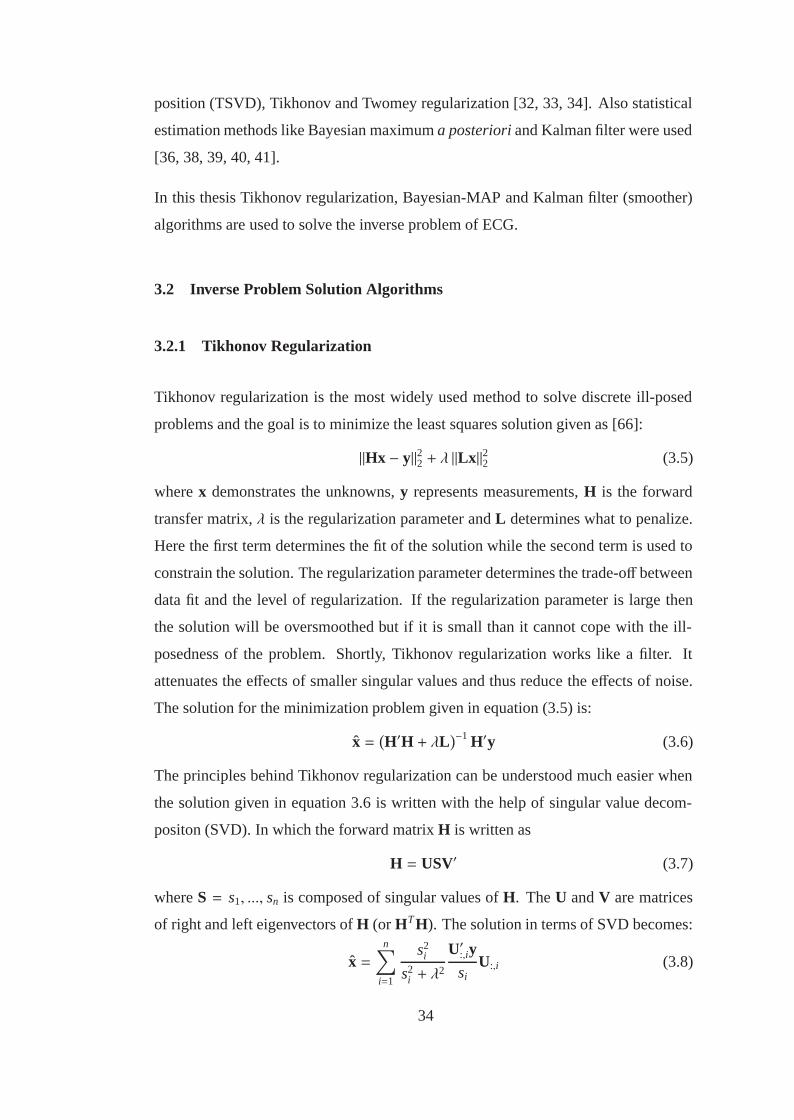
position (TSVD), Tikhonov and Twomey regularization [32, 33, 34]. Also statistical
estimation methods like Bayesian maximum a posteriori and Kalman filter were used
[36, 38, 39, 40, 41].
In this thesis Tikhonov regularization, Bayesian-MAP and Kalman filter (smoother)
algorithms are used to solve the inverse problem of ECG.
3.2 Inverse Problem Solution Algorithms
3.2.1 Tikhonov Regularization
Tikhonov regularization is the most widely used method to solve discrete ill-posed
problems and the goal is to minimize the least squares solution given as [66]:
‖Hx − y‖22 + λ ‖Lx‖22 (3.5)
where x demonstrates the unknowns, y represents measurements, H is the forward
transfer matrix, λ is the regularization parameter and L determines what to penalize.
Here the first term determines the fit of the solution while the second term is used to
constrain the solution. The regularization parameter determines the trade-off between
data fit and the level of regularization. If the regularization parameter is large then
the solution will be oversmoothed but if it is small than it cannot cope with the ill-
posedness of the problem. Shortly, Tikhonov regularization works like a filter. It
attenuates the effects of smaller singular values and thus reduce the effects of noise.
The solution for the minimization problem given in equation (3.5) is:
x =(H′H + λL
)−1 H′y (3.6)
The principles behind Tikhonov regularization can be understood much easier when
the solution given in equation 3.6 is written with the help of singular value decom-
positon (SVD). In which the forward matrix H is written as
H = USV′ (3.7)
where S = s1, ..., sn is composed of singular values of H. The U and V are matrices
of right and left eigenvectors of H (or HT H). The solution in terms of SVD becomes:
x =n∑
i=1
s2i
s2i + λ
2
U′:,iysi
U:,i (3.8)
34
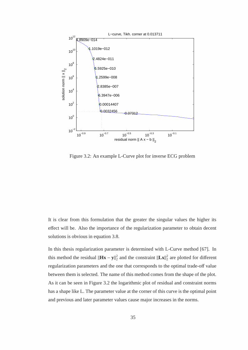
10−0.9
10−0.7
10−0.5
10−0.3
10−0.1
10−2
100
102
104
106
108
1010
1012
0.073120.0032456
0.00014407
6.3947e−006
2.8385e−007
1.2599e−008
5.5925e−010
2.4824e−011
1.1019e−012
4.8909e−014
residual norm || A x − b ||2
solu
tion
norm
|| x
||2
L−curve, Tikh. corner at 0.013711
Figure 3.2: An example L-Curve plot for inverse ECG problem
It is clear from this formulation that the greater the singular values the higher its
effect will be. Also the importance of the regularization parameter to obtain decent
solutions is obvious in equation 3.8.
In this thesis regularization parameter is determined with L-Curve method [67]. In
this method the residual ‖Hx − y‖22 and the constraint ‖Lx‖22 are plotted for different
regularization parameters and the one that corresponds to the optimal trade-off value
between them is selected. The name of this method comes from the shape of the plot.
As it can be seen in Figure 3.2 the logarithmic plot of residual and constraint norms
has a shape like L. The parameter value at the corner of this curve is the optimal point
and previous and later parameter values cause major increases in the norms.
35
3.2.2 Bayesian Maximum A Posteriori Estimation
In section 3.1 it is described that our goal is to find unknown x with given measure-
ments y. The x and y assumed as random variables. It is known from Bayesian phi-
losophy that when the prior probability density function (pdf) of an unknown random
variable p(x) is given along with its conditional pdf y given x (likelihood function),
the posterior conditional pdf x given y can be found from the equation below [68],
p(x\y) =p(y\x)p(x)∫
Xp(y\x)p(x)dx
(3.9)
where X is the parameter space.
In Bayesian-MAP the solution x that maximizes the posterior pdf is tried to be calcu-
lated:
x = argmaxxp(x\y) (3.10)
When the unknown x is assumed as epicardial potentials, the pdf of x can be assumed
as normally distributed with mean x and Covariance matrix with Cx. Also the mea-
surement noise v shown in equation (3.3) is assumed as independent and identically
distributed Gaussian noise, so its pdf is v ∼ N(0,R) where R = σ2vI. Therefore the
joint pdf is represented as [69]:
E
⎧⎪⎪⎪⎨⎪⎪⎪⎩⎛⎜⎜⎜⎜⎜⎜⎜⎝ x
y
⎞⎟⎟⎟⎟⎟⎟⎟⎠⎫⎪⎪⎪⎬⎪⎪⎪⎭ =⎛⎜⎜⎜⎜⎜⎜⎜⎝ x
Hx
⎞⎟⎟⎟⎟⎟⎟⎟⎠ (3.11)
Cx,y =
⎛⎜⎜⎜⎜⎜⎜⎜⎝ Cx CxH′
HCx HCxH′ + R
⎞⎟⎟⎟⎟⎟⎟⎟⎠ (3.12)
Under these conditions the solution to the maximization problem shown in equation
(3.10) can be obtained as:
x =(H′R−1H + C−1
x
)−1 (H′R−1y + C−1
x x)
(3.13)
More detail about the Bayesian-MAP can be found in [68, 69].
36
3.2.3 Temporal Bayesian-MAP
The Bayesian-MAP approach described in 3.2.2 assumes no temporal correlation be-
tween epicardial potentials and thus solve each time instant separately. But electrical
activity in the heart has temporal dependence too [13]. In order to include temporal
information to Bayesian-MAP solution the isotropy assumption is used which is sug-
gested by Greensite et al. [50, 47]. The isotropy is very similar to the separability
condition for random variables. According to separability condition a spatio-temporal
random variable’s cross-covariance matrix Cx depends on temporal covariance matrix
Ct and spatial covariance matrix Cs as shown below [47]:
Cx = Ct ⊗ Cs (3.14)
where ⊗ is the kronecker product and:
E[XX′] = Cs
N∑j=1
tCt( j, j) (3.15)
E[X′X] = Ct
N∑i=1
sCs(i, i) (3.16)
With X represents mean removed random variable.
From equations (3.15) and (3.16) Cx is written as:
Cx =E[X
′X] ⊗ E[XX
′]∑N
i=1 sCs(i, i)∑N
j=1 tCt( j, j)(3.17)
Due to high memory requirement of the direct solution the solution should be modi-
fied to a column by column solvable formulation as in the spatial Bayesian-MAP. For
that purpose the time correlation should be broken somehow. To break the the time
correlation temporal whitening can be used. This method is simply using a transfor-
mation matrix Z such that the new coordinate system supplies the time independency
that is required to solve the problem with spatial Bayesian-MAP. Then instead of
solving the whole system at once, it could be solved column by column. By that way
the memory consumption of the solution algorithm is reduced without ignoring the
time dependency.
37
Choosing an appropriate transformation matrix which supplies the time decorrelation
is very important to have minimum error using this assumption. For that purpose the
transformation matrix should be chosen as orthogonal and also it should diagonalize
E[Y′Y]. In previous studies that matrix (Z) is chosen as eigenvectors of E[Y′Y] and
at that study it is chosen the same [37].
This process is called temporal whitening and the modified model for this system
becomes [49]:
YZ = HXZ + VZ (3.18)
where V is the noise matrix with independent and identically distributed Gaussian
assumption. Also equation (3.17) for Cxz becomes:
Cxz =E[(XZ)′(XZ)] ⊗ E[(XZ)(XZ)′]
E[∥∥∥∥X∥∥∥∥2
F]
(3.19)
where ‖.‖2F is the Frobenius norm.
When the system given in equation (3.18) is solved column by column with Bayesian-
MAP formulation 3.13, the new unknown XZ is calculated. Finally using orthogo-
nality of the transformation matrix Z the estimate for X is determined from:
X = XZZ′ (3.20)
More information about these derivations could be found in papers [50, 47, 49].
3.2.4 Kalman Filter and Smoother
The first implementation of the Kalman filter was a part of the space program directed
by NASA (National Aeronautics and Space Administration) [70]. Since then the
Kalman filter is used for a variety of problems from economy to biology [71, 72].
The main reason is its optimality in the mean square error sense with given a priori
information and its ability to include uncertainties easily.
38

Using Kalman filter, processes that are represented with state space models can be
solved and the inverse ECG problem can be represented with a state space model as
shown in equations (3.2) and (3.3). Those equations are repeated below:
xk = Fxk−1 + wk (3.21)
yk = Hxk + vk (3.22)
The derivations given in this section are modified from the books [73, 74, 75].
The Kalman filter is an estimator used to determine the most probable unknown states
xkk and error covariance Pk
k with given measurements Yk = y1, ..., yk. Mathematically
xkk = E(xk|Yk) (3.23)
Pkk = E{(xk − xk
k)(xk − xkk)′} (3.24)
The Kalman filter is a two stage estimator. At the first stage a priori state estimation
xk−1k and error covariance Pk−1
k are estimated with measurement Yt−1 = y1, ..., yt−1
xk−1k = E(xk|Yk−1) = E(Fxk−1 + wk|Yk−1) = Fxk−1
k−1 (3.25)
Pk−1k = E{(xk − xk−1
k )(xk − xk−1k )′} = FPk−1
k−1F′ +Q (3.26)
At the second stage a priori state and error covariance that are shown in equations
(3.25) and (3.26) are updated with the measurement at the last time instant yk. For
that purpose first the innovations or residuals should be determined which are defined
as
εk = yk − E(yk|Yk−1) (3.27)
The expectation of residuals is zero and its variance is
var(εk) = HkPk−1k H′k + R (3.28)
So,
xkk = E(xk|Yk) = E(xk|Yk−1, εk) = xk−1
k +Kkεk (3.29)
Pkk = [I −KkHk]Pk−1
k (3.30)
39
A posteriori error covariance could also be calculated with a different formulation.
That formulation satisfies the need for Pkk to be positive definite and symmetric which
helps to avoid problems due to ill-conditioning.
Pkk = [I −KkHk]Pk−1
k [I −KkHk]′ +KkRkK′k (3.31)
It is clear that the formulation above satisfies both symmetry and positive definite-
ness requirements. The symmetry is satisfied because the formulation compose of
summation of two symmetric matrices so the result is symmetric too. Also the first
term is a positive definite matrix and the second term is a nonnegative definite matrix
whose sum is obviously a positive definite matrix [73]. In equation (3.31) Kk is the
Kalman gain that decides the amount of correction to a priori estimates using the last
measurement and formulated as:
Kk = Pk−1k H′k(HkPk−1
k H′k + R)−1 (3.32)
Equations (3.25), (3.26), (3.29), (3.31) and (3.32) are called the Kalman filter equa-
tions. This formulation is called Kalman filter because it uses all measurements up to
the time instant that the state is going to be calculated. For example xk is calculated
with Yk. If xk was calculated from Yk−1, it would be called an estimator. Actually
equations (3.25) and (3.26) are estimation. Also if xk is calculated from all measure-
ments such that Yn (where n is bigger than k) then it is called Kalman smoother. It
is called smoother because the results are usually smoother than the filter results. In
this study also Kalman smoother is used to further decrease errors.
The Kalman smoother does the backward recursion and requires the results of Kalman
filter for the last time instant (xnn, Pn
n). Those equations to obtain Kalman smoother
are given as:
Jk−1 = Pk−1k−1F′[Pk−1
k ]−1 (3.33)
xnk−1 = xk−1
k−1 + Jk−1(xnk − xk−1
k ) (3.34)
Pnk−1 = Pk−1
k−1 + Jk−1(Pnk − Pk−1
k )J′k−1 (3.35)
where k = n, ..., 1
40
3.2.5 Determination of STM for Kalman Filter from Epicardial Potentials
For standard Bayesian-MAP and Tikhonov regularization algorithms only equation
(3.2) is used but for Kalman filter approach also the equation (3.3) is used and the ma-
trix F which is called state transition matrix (STM) should be determined. As can be
seen from equation (3.3) STM maps the unknown states (epicardial potentials) at the
previous time instant to the states at the next time instant thus contains the temporal
information regarding the problem. For that reason unlike standard Bayesian-MAP
and Tikhonov regularization techniques Kalman filter is a spatio-temporal method.
To obtain a decent solution with Kalman filter the correctness of the STM is very
important. But the determination of it for inverse ECG problem is not an easy task. In
this subsection the technique that is suggested by Goussard et al. [39] is explained. In
this technique the epicardial potentials are used to determine the STM. For that pur-
pose they changed the formulation and assumed the epicardial potentials are known
and it is STM which should be determined. Then they solved this formulation with a
modified version of Kalman filter.
The new formulation where the unknown states are the elements of the STM is as:
xk = Xk−1f + wk (3.36)
Where,
f =
⎛⎜⎜⎜⎜⎜⎜⎜⎜⎜⎜⎜⎜⎜⎜⎜⎜⎜⎜⎜⎜⎜⎜⎝
f1
f2
...
fN
⎞⎟⎟⎟⎟⎟⎟⎟⎟⎟⎟⎟⎟⎟⎟⎟⎟⎟⎟⎟⎟⎟⎟⎠, X (k) =
⎛⎜⎜⎜⎜⎜⎜⎜⎜⎜⎜⎜⎜⎜⎜⎜⎜⎜⎜⎜⎜⎜⎜⎝
x′(k) 0 · · · 0
0 x′(k) · · · 0
......
. . ....
0 0 · · · x′(k)
⎞⎟⎟⎟⎟⎟⎟⎟⎟⎟⎟⎟⎟⎟⎟⎟⎟⎟⎟⎟⎟⎟⎟⎠(3.37)
In equation 3.37 fN is the transpose of the N’th row of STM matrix and xT(k) is the
transpose of the epicardial potentials at time instant k.
As stated previously a modified version of Kalman Filter is used to solve this problem
which is given as [39]:
Kk = PkX′k (3.38)
fk+1 = fk +KkQ−1 (xk+1 − Xkfk) (3.39)
41

Qk = I + XkPkX′k (3.40)
Pk+1 = Pk −KkQ−1k K′k (3.41)
After rearranging the f as STM matrix, it could be used in Kalman Filter. For more
detail on these one may refer to [39].
In this equation 3.41 K is the Kalman gain, Q is the covariance matrix of noise and P
is the error covariance matrix.
This technique’s high memory requirement is a major drawback. For an array of
sensors that have measurements from 490 sensors the size of the error covariance
matrix P becomes a matrix with size 4902x4902 that requires approximately 429 GB
of memory. In their work Goussard et. al. use the locality property to reduce the
dimension of the problem by assuming a node is associated to only its neighbors.
To avoid high memory problem we use the activation times of the nodes along with
locality properties.
For that purpose first the activation time of each node is calculated using the second
order differentials. Then the epicardial potential value at node (i) in time instant (k)
is assumed as dependent to only the nodes at time instant (k-1) whose activation
times are closed to the i’th. Only the elements of STM and so f that corresponds to
those nodes are calculated and others are forced to zero. The rows of X in equation
3.37 corresponding to the elements that will be forced to zero at f has no effects on
the calculated STM. For that reason those rows are deleted from the matrix which
also reduces size of error covariance matrix at modified Kalman filter form N2xN2
to NDxND where N is the number of nodes on epicardium and D is the number of
nodes that are assumed as associated to each other for each node. By benefiting from
this property the memory consumption could be significantly reduced.
Usage of activation times also allow us to include physiological information to our
problem solution. For example the nodes with close activation times probably cor-
responds to the fiber directions on the heart and so if the fiber directions are known
the nodes that will be associated to each other could have chosen according to this
information. This might save us from the obligation to calculate activation times for
each node while introducing physiological constraints.
42
3.3 Enhanced Noise Model for Geometric Error Compensation
Modeling errors are very often in inverse problems. For inverse ECG problem those
modeling errors may be due to discretization, wrong interpretation of electrode lo-
cations, wrong determination of heart’s size and location and wrong conductivity
assignments in the mathematical torso model. In the literature it can be seen that ge-
ometric errors have very significant effects in solutions [28]. As a part of this thesis
geometric errors occur due to wrong size and location assignments to the heart are
investigated. The effects of those geometric errors are also tried to be minimized with
the modification of a method suggested by Kaipio et. al. for inverse problem solu-
tions [76]. This model was implemented to optical tomography before [77] but to the
best of our knowledge this is the first study that modifies this method to the inverse
problem of electrocardiography.
In order to consider geometric errors the formulation of the system is changed as:
y = H(x, z) + v (3.42)
The difference in this formulation from others is that the transfer matrix is assumed as
dependent on parameter vector z. For inverse electrocardiography problem those pa-
rameters are the size and locations of each tissue that are present in the mathematical
torso model.
If the true parameter vector is assumed as z* and the parameter vector that are used
in the inverse model are represented by z, then it is clear that extra errors enter the
system. For that case the formulation becomes [77]:
y = H(x, z*) + (H(x, z) −H(x, z*)) + v (3.43)
In the formulation above (H(x, z) − H(x, z*)) term represents the error due to uncer-
tainties in the parameters of the transfer matrix. Those uncertainties may be due to
wrong interpretations of the heart’s size and location and thus this error represents
the geometric errors in the problem. If that noise is assumed as ε(x, z) then equation
(3.43) becomes [77]:
43
y = H(x, z*) + ε(x, z) + v (3.44)
For simplicity H is assumed as linearly dependent to parameters z and using Gaussian
approximation geometric error is written as [77]:
ε(x, z) = DzH(x, z*)δz (3.45)
With,
δz = z − z∗ (3.46)
In the formulation above Dz is the Jacobian matrix with respect to z. If the expectation
of the geometric error is assumed as zero then the covariance of the geometric error
is [77]:
E(ε(x, z)ε(x, z)′
)= Γε = DzH(x, z*)ΓzDzH(x, z*)′ (3.47)
where,
Γz = E(δzδ′z)
(3.48)
Finally, benefiting from the independence assumption between geometric errors and
measurement noise equation (3.43) is written as:
y = H(x, z∗) + e (3.49)
With the covariance matrix of e is Γe = Γε + Γv.
More detail on the proofs given in this part can be found in Kaipio et. al.’s book and
journal so interested reader is encouraged to read those [77, 76].
To summarize, ENM allows the usage of Γe instead of measurement noise covariance
R to reduce the effects of geometric errors in the inverse ECG problem.
44
3.4 System Identification Problem
The usage correct values of measurement and process noise covariances is critical to
obtain decent solutions with inverse solution algorithms. In this section two different
methods are described to determine the noise covariances for inverse ECG problem.
The first method benefits from residuals and the other one uses expectation maximiza-
tion. Those methods do not only used to calculate noise covariance matrices under
normal conditions but also in the case of geometric errors. In that sense those methods
are used to determine the noise covariances employed in enhanced noise model.
3.4.1 Determination of Measurement and Process Noise Covariance Matrices
Using Residuals
As stated in 3.2.4 the values of measurement (R) and process (Q) covariance matrices
should be known to use Kalman filter. As a part of this thesis those covariances are
calculated from the residuals for inverse ECG problem such as Bailie and Jazwinski
propose for orbit determination problem [78].
To calculate the noise covariances, first the residual should be calculated as:
rk = y(i)k −H(i)xk−1k (3.50)
R(i)k = r2k −H(i)Pk
kH(i)′ (3.51)
where i represents the row number and k is used to show time instant. So H(i) repre-
sents the i’th row of the forward transfer matrix. On the equations above if the value
of R(i)k is not positive then its value should be assigned as 0 [78]. Then xkk, Pk
k and
xk+1k are calculated with Kalman filter equations as [78]:
xkk = xk−1
k + Pk−1k H(i)′(H(i)Pk−1
k H(i)′ + R(i)k)−1(y(i)k −H(i)xk−1
k ) (3.52)
Pkk = Pk−1
k − Pk−1k H(i)′(H(i)Pk−1
k H(i)′ + R(i)k)−1H(i)Pk−1
k (3.53)
xkk+1 = Fxk
k (3.54)
After the residual for k+1’th time instant is calculated from the formula given in
equation (3.50), the process noise covariance elements are calculated as [78]:
45

Q(i)k =rk+1 −H(i)FPk
kH(i)′ + R(i)k
H(i)H(i)′(3.55)
Again non-positive elements of covariance matrix are forced to zero. Finally error
covariance matrix Pkk+1 is calculated with formulation below and the process contin-
ues.
Pkk+1 = FPk
kF′ +Q(i)k (3.56)
More detail regarding the general formulations in this section can be found in [78].
3.4.2 Determination of Measurement and Process Noise Covariances Using Ex-
pectation Maximization
In this technique the likelihood is tried to be maximized for parameters Θ = [Q,R]
[75, 79]. In expectation maximization (EM) algorithm the complete data likelihood
with Gaussian assumption is written as [75, 79]:
−2lnLX,Y(Θ) = ln |Σ0| + (x0 − μ)′Σ−10 (x0 − μ)
+ ln |Q| +n∑
k=1
(xk − Fxk−1)′Q−1(xk − Fxk−1)
+ ln |R| +n∑
k=1
(yk −Hxk)′R−1(yk −Hxk) (3.57)
where Σ and μ are the covariance and mean of the initial state vector x0. In EM
algorithm maximizing the conditional expectation of the complete data likelihood
with iterations is same as maximizing complete data likelihood. So at the j-th iteration
[75, 79]:
Q(Θ|Θ( j−1)) = E{−2lnLX,Y(Θ)|Yn,Θ
( j−1)}
(3.58)
The procedure have 4 steps and the iterations are j = 1, 2, ...
1. Initial parameter values Θ(0) = [Q,R] are selected along with μ and Σ
2. The expectation step is performed. In this step the Kalman smoother estima-
tions are used to calculate S11, S10 and S00 which forms the conditional expec-
46

tation of the complete data likelihood as below:
Q(Θ|Θ( j−1)) = ln |Σ0| + tr{Σ−1
0 [Pn0(xn
0 − μ0)(xn0 − μ0)′]
}+ ln |Q| + tr
{Q−1[S11 − S10F′ − FS′10 + FS00F′]
}+ ln |R| + tr
⎧⎪⎪⎨⎪⎪⎩R−1n∑
k=1
(yk −Hxnk)′ +HPn
kH′⎫⎪⎪⎬⎪⎪⎭ (3.59)
With S11, S10 and S00 are as
S11 =
n∑k=1
(xnkxn
k′ + Pn
k) (3.60)
S10 =
n∑k=1
(xnkxn
k−1′ + Pn
k,k−1) (3.61)
S00 =
n∑k=1
(xnk−1xn
k−1′ + Pn
k−1) (3.62)
The Pnk,k−1 is found using the lag-one covariance smoother whose formulation
is as for k = n, n − 1, ..., 2 [75, 79]:
Pnk−1,k−2 = Pk−1
k−1J′k−2 + Jk−1(Pnk,k−1 − FPk−1
k−1)J′k−2 (3.63)
With initial value as
Pnn,n−1 = (I −KnH)FPk−1
k−1 (3.64)
3. In this step as the name expectation maximization implies the expectation is
tried to be maximized for parameters. SoΘ( j) is calculated with equations given
below [75, 79]:
Q( j) = n−1(S11 − S10S−100 S′10) (3.65)
R( j) = n−1n∑
k=1
[(yk −Hxnk)′ +HPn
kH′] (3.66)
4. Next iteration starts from the second step with new parameter values.
More information about derivations can be found in [75, 79].
47

CHAPTER 4
RESULTS AND DISCUSSION
In this chapter first the data used for simulations are explained and then the recon-
struction results for inverse problem of electrocardiography are given.
4.1 Simulated Data
The body surface potential measurements used in this study are simulated using the
QRS intervals of measured epicardial potentials and an appropriate noise and forward
model which is explained in detail later.
The epicardial potentials used for this study are measured at University of Utah Nora
Eccles Harrison Cardiovascular Research and Training Institute (CVRTI) [56]. The
measurements are taken from a dog heart which is perfused from another dog’s cir-
culatory system and suspended in an electrolytic filled (500Ωcm) adolescence human
thorax shaped fiberglass tank. To measure the epicardial potentials a nylon sock elec-
trode with silver wires is slipped over the ventricles. During measurements the heart
is stimulated from the ventricles to simulate ventricular arrhythmias. The epicardial
measurements are taken from 64 or 490 points with sampling rate 1000 sample per
second.
The forward transfer matrix that maps epicardial potentials to body surface potentials
is calculated with boundary element method from MRI images 1. The thorax model
consists of heart, torso and lungs. The conductivity values for thorax volume and
lungs are taken from literature as 0.0002 S/mm and 0.00005 S/mm respectively [60].
1 The forward solver is developed by Dr. Ozlem Birgul
48

Figure 4.1: Schematic representation of the forward problem.
The forward transfer matrix is used to obtain 658 or 771 body surface potentials form
epicardial potential measurements from 64 or 490 points respectively.
The body surface potentials are obtained from the epicardial potential measurements
by a multiplication with the transfer matrix and addition of 30 dB SNR independent
and identically distributed Gaussian noise. By doing so the forward problem of elec-
trocardiography is solved. This process is shown in Figure 4.1.
4.2 Validation Methods
The quantitative comparisons of the solutions are made using correlation coefficients
(CC) and relative difference measurement star (RDMS):
CC =N(∑T
i=1 XiXi
)−(∑T
i=1 Xi
) (∑Ti=1 Xi
)√
N(∑T
i=1 X2i
) (∑Ti=1 Xi
)2√N(∑T
i=1 X2
i
) (∑Ti=1 Xi
)2 (4.1)
49
RDMS =
√√√√∑⎛⎜⎜⎜⎜⎜⎜⎝ Xi∑Ti=1 X
2
i
− Xi∑Ti=1 X2
i
⎞⎟⎟⎟⎟⎟⎟⎠2
(4.2)
As it is clear from their formulations that higher CC and lower RDMS correspond
to better solutions. Although RDMS and CC give us information about the perfor-
mances of the methods used for inverse electrocardiography problem, it is also im-
portant to compare original and reconstructed epicardial distributions visually. One
of the reasons for this visual comparison is that the error measures used in this study
cannot put necessary emphasis on true reconstruction of activation wavefront which is
one of the most important features for inverse electrocardiography problem. For that
purpose map3d software has been used which is a scientific visualization application
written in Utah Nora Eccles Harrison Cardiovascular Research and Training Institute
for the purpose of displaying and editing three-dimensional geometric models and
time-based data associated with those models [80].
In Figure 4.2 the epicardial potential distribution and body surface potential map for
a certain time instant which are plotted by map3d software are shown. In this fig-
ure red represents the regions that have not activated yet and the blue regions show
the cells that have already been activated, the transition region between those two is
the activation wavefront. While the results are compared with map3d two important
characteristics are considered:
1. The solution’s ability to follow the wavefront without dispersing it much. The
dispersion in the wavefront is due to the regularization.
2. The solution’s ability to correctly reconstruct the activated or inactivated re-
gions.
50

Figure 4.2: Sample epicardial and body surface potential potential maps plotted withmap3d [80] for a certain time instant.
4.3 Reduction of the Problem Size for Inverse ECG Solution Using Kalman
Filter
4.3.1 Comparison of the Reduced Formulation for STM Calculation with the
Original One for 64 Node Data
In this subsection the algorithm suggested by Goussard et al. is implemented with
some modifications to improve its performance. As explained in 3.2.5 they calcu-
lated the state transition matrix (STM) from epicardial potential (EP) measurements.
The drawback of this approach is the high dimension of the problem when all nodes
are assumed as related to each other. For example for N EP nodes the size of the error
covariance matrix for full STM calculation algorithm is N2xN2. Although it could be
calculated for 64 nodes (the memory requirement for error covariance matrix is 128
MB) for a model with higher resolution such as 490 epicardial nodes the memory re-
quirement is approximately 430 GB. For that purpose Goussard et al. tries to benefit
from the locality property of the problem and construct the STM as the EP at one
time instant is related to only its 4 closest neighbors at the previous time instant. This
assumption reduce the problem dimension significantly but introduce extra errors. In
this part of the thesis we benefit from other characteristics of the propagating activa-
tion wavefront to achieve the reduction in the problem dimension without introducing
extra errors. For that purpose strategies explained below are tested and a sample illus-
tration of the nodes that corresponds to the scenarios explained are shown at Figure
4.3.
51

1. All nodes are assumed as related to each other which is called here as the full
STM approach.
2. Only the first order neighbors are assumed as related to each other (approxi-
mately 7 node for each node).
3. Only the second order neighbors are assumed as related to each other (approx-
imately 18 node for each node).
4. Only the nodes with close activation times are related to each other (within 11
ms threshold approximately 18 node).
5. The union set of the nodes that are found from both 1’st and 3’rd approaches
are related to each other (within 4 ms threshold).
At this point extra information for the 3’rd and 4’th strategies might be needed. The
motivation behind using those two strategies is to benefit from the relation between
the signals that are along the same wavefront. In order to use those strategies at first
the activation times for each node are determined by using the second derivative’s of
the EP’s. The goal here is to relate those leads that are located on the same wavefront;
i.e., those that are depolarized at the same time. For that purpose the activation time
difference for each node is calculated and the nodes whose activation time difference
are within a predetermined threshold are related to each other. The STM is calculated
only for the entries that corresponds to those predetermined related nodes and other
entries are forced to zero.
In this part of the study the STM is calculated from the test data itself. After the
STM’s are calculated according to the 5 scenarios, the inverse solutions are obtained
by processing the data first with Kalman filter and then with Kalman smoother. The
schematic representation of the simulation procedure is shown at Figure 4.4.
At the first step the simulations are conducted with EP measurements from 64 nodes
to test the performances of the strategies 2 to 5 compared to the calculation in which
full STM is used (strategy 1).
52
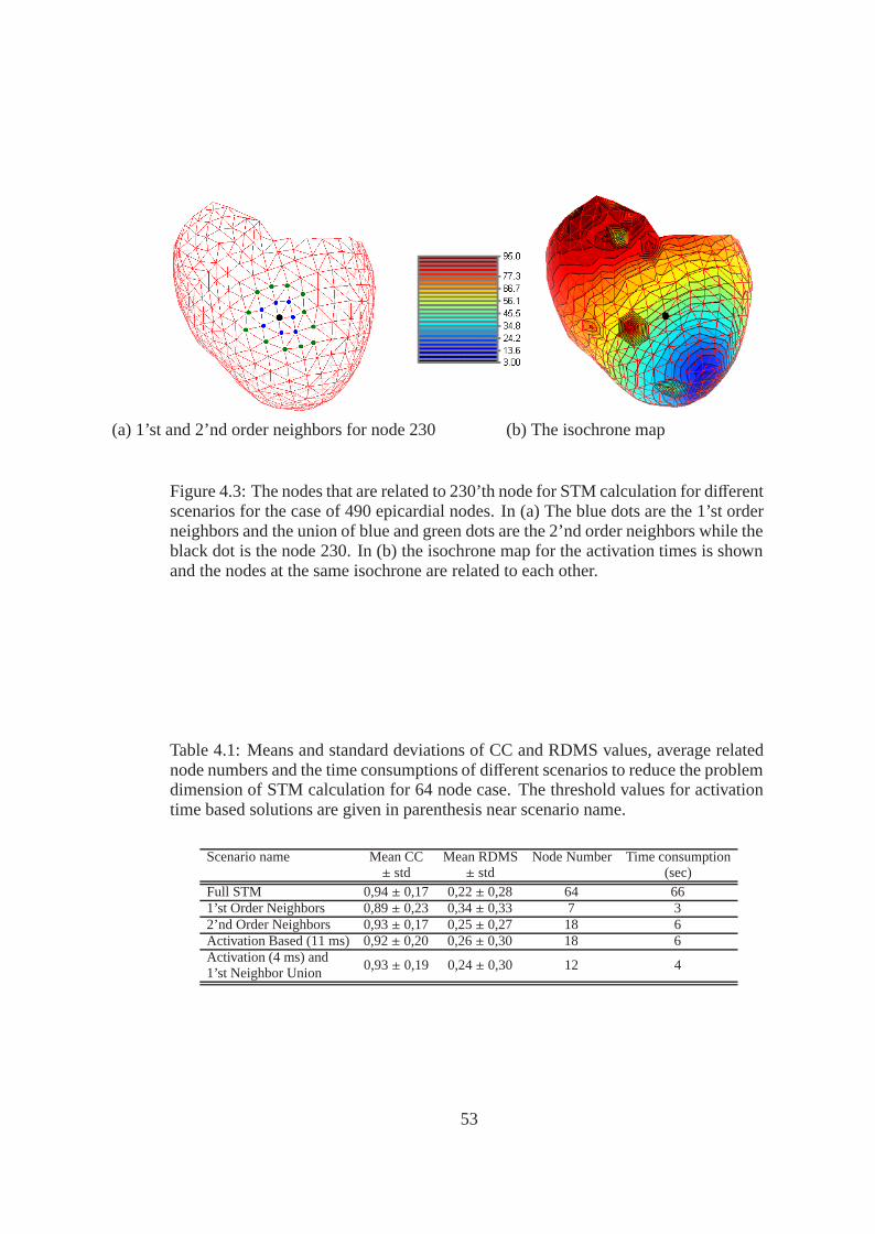
(a) 1’st and 2’nd order neighbors for node 230 (b) The isochrone map
Figure 4.3: The nodes that are related to 230’th node for STM calculation for differentscenarios for the case of 490 epicardial nodes. In (a) The blue dots are the 1’st orderneighbors and the union of blue and green dots are the 2’nd order neighbors while theblack dot is the node 230. In (b) the isochrone map for the activation times is shownand the nodes at the same isochrone are related to each other.
Table 4.1: Means and standard deviations of CC and RDMS values, average relatednode numbers and the time consumptions of different scenarios to reduce the problemdimension of STM calculation for 64 node case. The threshold values for activationtime based solutions are given in parenthesis near scenario name.
Scenario name Mean CC Mean RDMS Node Number Time consumption± std ± std (sec)
Full STM 0,94 ± 0,17 0,22 ± 0,28 64 661’st Order Neighbors 0,89 ± 0,23 0,34 ± 0,33 7 32’nd Order Neighbors 0,93 ± 0,17 0,25 ± 0,27 18 6Activation Based (11 ms) 0,92 ± 0,20 0,26 ± 0,30 18 6Activation (4 ms) and
0,93 ± 0,19 0,24 ± 0,30 12 41’st Neighbor Union
53
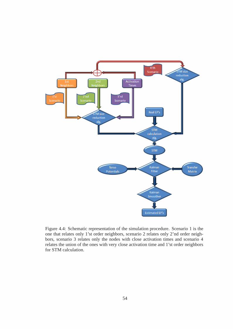
Figure 4.4: Schematic representation of the simulation procedure. Scenario 1 is theone that relates only 1’st order neighbors, scenario 2 relates only 2’nd order neigh-bors, scenario 3 relates only the nodes with close activation times and scenario 4relates the union of the ones with very close activation time and 1’st order neighborsfor STM calculation.
54

−1 −0.8 −0.6 −0.4 −0.2 0 0.2 0.4 0.6 0.8 1−1
−0.8
−0.6
−0.4
−0.2
0
0.2
0.4
0.6
0.8
1
Full STM1st Neigh2nd NeighActivationAct−Neigh
RDMS
CC
Time Cons.
Figure 4.5: Starchart representation of time consumption, CC and RDMS.
In Table 4.1 the averages of CC and RDMS for the previously described strategies are
given. The node number shows the average number of nodes that are related to one
node. This number also corresponds to the average number of non-zero entries of the
STM for one row. It can be seen that full STM approach has the best error perfor-
mance. But other approaches except the one that uses 1’st order neighbors, have very
similar performances to full STM approach, although the problem dimension and
computation time are significantly decreased. The reason for this result can be under-
stood when the entries of the full STM is studied. In full STM most of the entries are
so close to zero which means that they have no significant relation for the correspond-
ing nodes. Also if the entries with the highest values are checked it can be seen that
the nodes that correspond to those entries are not only the neighbors. Sometimes the
entry corresponding to two nodes with far locations is very high which contradicts to
the assumption of using only the locality property of the activation wavefront propa-
gation. When those related nodes are studied further, a pattern appears and it can be
seen that those nodes are the ones that are along the same activation wavefront. This
result also demonstrates the logic behind using not only local neighbors but also the
55

ones with close activation times. The same results could be observed from Figure 4.5
too. At that chart CC, RDMS and time consumption of the algorithms are plotted on
three dashed lines with 120 degree between them. In this plot the algorithm which
crosses the dashed line at the outer most point has the best performance in the criteria
that dashed line represents.
The interpretations made for Table 4.1 are also verified by Figure 4.6. This figure
shows the epicardial distributions calculated at 37 ms after the stimulation with the
scenarios described previously. Those results also indicate that there is no obvious
difference between using the full STM, 2’nd order neighbor, activation based and
activation union 1’st neighbor scenarios. Close correspondence of those solutions to
the real epicardial potential distribution is also observed.
The results presented here show that the inverse problem of ECG could be solved
without using the full STM because most of the entries of that STM is very close to
zero. Also the nodes that should be related to each other can be determined bene-
fiting from not only the locality property but also the shape of the wavefront. One
possible question is how to determine those nodes along the same wavefront for real
case. There are two possible answers to this question. The first one is, the approxi-
mate activation times could be determined from the pre-solutions obtained with other
methods like Bayes-MAP or Tikhonov regularization and and the second one is, if
the fiber directions are known the nodes along those fiber directions could be used as
those along the same activation wavefront.
4.3.2 Comparison of the Proposed Problem Dimension Reduction Techniques
for STM Calculation with 490 Node Data
The reason for using the data with 64 epicardial nodes previously was to assess the
performance when problem dimension is reduced and the results show no significant
reduction in the performance. Here those scenarios except the full STM scenario (due
to its very high computational cost) ,for a problem with higher resolution which tries
to find the EP’s from 490 nodes using BSP’s from 771 nodes, are tested.
The simulation procedure is same as in subsection 4.3.1 and only the threshold values
56
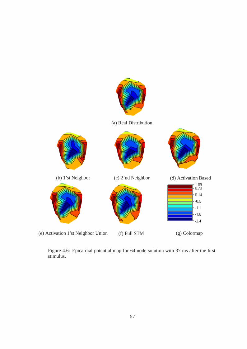
(a) Real Distribution
(b) 1’st Neighbor (c) 2’nd Neighbor (d) Activation Based
(e) Activation 1’st Neighbor Union (f) Full STM (g) Colormap
Figure 4.6: Epicardial potential map for 64 node solution with 37 ms after the firststimulus.
57
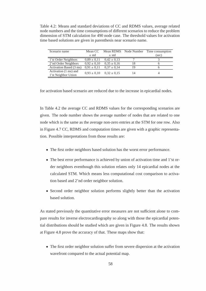
Table 4.2: Means and standard deviations of CC and RDMS values, average relatednode numbers and the time consumptions of different scenarios to reduce the problemdimension of STM calculation for 490 node case. The threshold values for activationtime based solutions are given in parenthesis near scenario name.
Scenario name Mean CC Mean RDMS Node Number Time consumption± std ± std (sec)
1’st Order Neighbors 0,89 ± 0,11 0,42 ± 0,13 7 32’nd Order Neighbors 0,92 ± 0,10 0,35 ± 0,16 18 6Activation Based (3 ms) 0,91 ± 0,11 0,37 ± 0,14 19 6Activation (1 ms) and
0,93 ± 0,10 0,32 ± 0,15 14 41’st Neighbor Union
for activation based scenario are reduced due to the increase in epicardial nodes.
In Table 4.2 the average CC and RDMS values for the corresponding scenarios are
given. The node number shows the average number of nodes that are related to one
node which is the same as the average non-zero entries at the STM for one row. Also
in Figure 4.7 CC, RDMS and computation times are given with a graphic representa-
tion. Possible interpretations from those results are:
• The first order neighbors based solution has the worst error performance.
• The best error performance is achieved by union of activation time and 1’st or-
der neighbors eventhough this solution relates only 14 epicardial nodes at the
calculated STM. Which means less computational cost comparison to activa-
tion based and 2’nd order neighbor solution.
• Second order neighbor solution performs slightly better than the activation
based solution.
As stated previously the quantitative error measures are not sufficient alone to com-
pare results for inverse electrocardiography so along with those the epicardial poten-
tial distributions should be studied which are given in Figure 4.8. The results shown
at Figure 4.8 prove the accuracy of that. These maps show that:
• The first order neighbor solution suffer from severe dispersion at the activation
wavefront compared to the actual potential map.
58
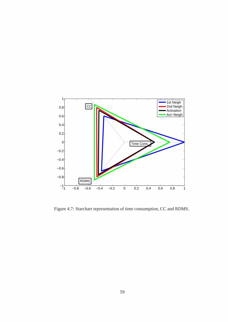
−1 −0.8 −0.6 −0.4 −0.2 0 0.2 0.4 0.6 0.8 1−1
−0.8
−0.6
−0.4
−0.2
0
0.2
0.4
0.6
0.8
1
1st Neigh2nd NeighActivationAct−Neigh
RDMS
CC
Time Cons.
Figure 4.7: Starchart representation of time consumption, CC and RDMS.
59

• The second order neighbor solution reduce the dispersion at the activation wave-
front but still the smoothing affect is obvious.
• The activation based solution does not have the activation wavefront dispersion
problem from which both first and second order neighbor solutions suffer. But
this approach suffers from another problem which is the false activated regions
that do not exist neither in the actual map nor in the neighborhood based mod-
els.
• The union of activation and first neighbor solution seems to benefit from the
advantages of both neighborhood and activation based methods. It follows the
wavefront much better than neighborhood based methods and does not have the
false activated areas reconstructed in the activation based method.
From Table 4.2 the second order neighbor method seems to perform better in error
metrics compared to the activation based method but from Figure 4.8 it is seen that
the activation time based method constructs the wavefront better. The reason for this
is quite simple. The neighborhood based methods result in spatial smoothing due
to the locality they benefit from so the activation wavefront is also smoothed along
with the inactivated and activated regions. The activation time based method is not
affected from this smoothing because it relates only those nodes that are on the same
activation wavefront. But due to the lack of the spatial smoothing the false regions
are not corrected in the activated and inactivated regions. On the other hand the union
of activation and first order neighbor avoids the smoothing at the wavefront due to
the related activation nodes and it avoids the false regions at activated or inactivated
regions with benefiting from the spatial smoothing of first order neighbors.
The conclusion of this part of the study is neither neighborhood nor activation based
methods are the best choices alone to determine nodes that should be related to each
other for STM determination. The best choice is using both of them which results in
better solutions with very significant reduction at the computational cost.
60
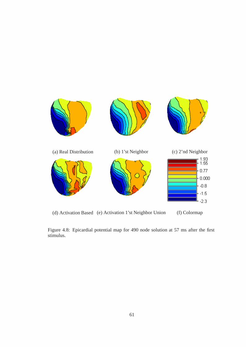
(a) Real Distribution (b) 1’st Neighbor (c) 2’nd Neighbor
(d) Activation Based (e) Activation 1’st Neighbor Union (f) Colormap
Figure 4.8: Epicardial potential map for 490 node solution at 57 ms after the firststimulus.
61

4.4 Studies on the Calculation of State Transition Matrix without Using Real
Epicardial Potentials
In the previous section the emphasis was on the reduction of the problem dimension
to calculate the STM. The STM’s calculated in the previous section requires the epi-
cardial potential distributions of the test data itself which is obviously not possible
in a realistic application. Those studies are helpful to show us that if appropriate
a priori information can be acquired the STM calculation described at the previous
section could be used to solve inverse electrocardiography problem with very high
correlations.
In this section our objective is to present ways to obtain the a priori information
needed to calculate the STM and compare those results with other spatial and spatio-
temporal techniques. For that purpose we have used the following techniques:
1. Bayes-Train: The spatial Bayes-MAP solution obtained using the mean and
covariance from the training set
2. Tikhonov: The zero’th order Tikhonov regularization solution
3. Temp-Bayes: The spatio-temporal Bayes-MAP solution with a priori informa-
tion from the training set
4. Kalman-Bayes: The training set is used to obtain the solution using the spatial
Bayes-MAP (Bayes-Train) and then this solution is used to calculate STM.
5. Kalman-Tikh: The solution of zero’th order Tikhonov regularization is used
to calculate STM.
6. Kalman-Direct: A training set is used to calculate the STM directly which is
suggested by Goussard et al. [39]
The BSP’s that are used for inverse solutions are produced same as previous section.
So epicardial potentials from 490 nodes are multiplied with the transfer matrix cal-
culated with BEM and finally 30 dB white Gaussian noise is added to obtain noisy
BSP’s.
62
The training set used at this study is constructed from 8 different epicardial potential
distributions which contains only the QRS intervals, with duration of 97 ms. The
epicardial potential maps used in training set are all stimulated from the ventricles
of the same dog heart but the location of the first stimulus site is different for each
of them so the epicardial potential distributions are different. The test data is not
included to the training set. The construction of training set for Bayes-Train and
Kalman Direct differs from the temporal training set used for Temp-Bayes.
The 490x776 training set Xs for Bayes-Train is constructed by adding the epicardial
potential distribution for each data column by column as shown below.
Xs = [X1 X2 · · · X8] (4.3)
Where 490x97 matrix Xi is the matrix that contains epicardial potential maps at 97
different time instants of the QRS interval for the i’th beat in the training set. The
number of columns at Xi represents the number of time instants at which the epicardial
potentials are measured and the number of rows are equal to the number of nodes on
the epicardium. The priori mean for each node is found by averaging the rows of the
training set over time and covariance matrix is found from equation given below.
Cs =XsXT
s
NT(4.4)
Where NT is the total number of time instants, which is 8x97 = 776. In this study it
is clear that the resulting 490x490 covariance matrix Cs contains only spatial infor-
mation.
For the Temp-Bayes algorithm the temporal covariance matrix Ct is also needed along
with the spatial covariance matrix Cs. In order to construct the 3920x97 training set Xt
for temporal information, the 490x97 Xi epicardial potential map matrices are added
row by row so:
Xt =
⎡⎢⎢⎢⎢⎢⎢⎢⎢⎢⎢⎢⎢⎢⎢⎢⎢⎢⎢⎢⎢⎢⎢⎣
X1
X2
...
X8
⎤⎥⎥⎥⎥⎥⎥⎥⎥⎥⎥⎥⎥⎥⎥⎥⎥⎥⎥⎥⎥⎥⎥⎦(4.5)
63
Then the temporal training set Ct is calculated with the formulation below:
Ct =XtXT
t
NS(4.6)
where NS is the row number of Xt and corresponds to the number of epicardial nodes.
The regularization parameter for zero’th order Tikhonov regularization is calculated
using the L-Curve method [67] and a different regularization parameter is used for
each time instant.
For Kalman-Bayes solution first the Bayes-Train solution is obtained. Then the epi-
cardial potential map obtained from those are assumed as the real epicardial potential
map and the activation time for each node is calculated from those. Finally the STM
is calculated with using the problem dimension reduction technique described in 4.3.
The procedure for Kalman-Tikh is the same as Kalman-Bayes only this time the so-
lution of Tikhonov is used to find the STM instead of Bayes-Train.
The Bayes-Train and Tikhonov algorithms benefit from only spatial information to
constrain the solution so these are called as spatial methods. On the other hand
Kalman-Direct, Kalman-Bayes, Kalman-Tikh and Temp-Bayes benefit from both tem-
poral and spatial constraints so those are spatio-temporal constraints. In this section
also spatial and spatio-temporal methods are compared for the solution of inverse
electrocardiography problem.
The schematic representation of the simulation procedure for methods Bayes-Train,
Tikhonov, Kalman-Bayes, Kalman Tikh and Kalman-Direct is given at Figure 4.9
In Table 4.3 the average CC and RDMS values obtained for the algorithms explained
above are given. In Figure 4.10 the performances of the algorithms in terms of CC,
RDMS and computation time are shown. At this plot the algorithm which crosses the
dashed line at the outer most point has the best performance in the criteria that dashed
line represents. The interpretations from this table and plot are:
• Tikhonov solution has the worst performance in terms of error metrics.
64

Figure 4.9: Schematic representation of the simulation procedure for Bayes-Train,Tikhonov, Kalman-Bayes, Kalman-Tikh and Kalman-Direct approaches
65
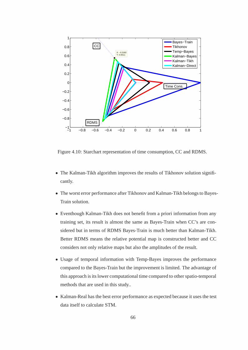
−1 −0.8 −0.6 −0.4 −0.2 0 0.2 0.4 0.6 0.8 1−1
−0.8
−0.6
−0.4
−0.2
0
0.2
0.4
0.6
0.8
1
X: −0.3182Y: 0.5511
Bayes−TrainTikhonovTemp−BayesKalman−BayesKalman−TikhKalman−Direct
Time Cons.
RDMS
CC
Figure 4.10: Starchart representation of time consumption, CC and RDMS.
• The Kalman-Tikh algorithm improves the results of Tikhonov solution signifi-
cantly.
• The worst error performance after Tikhonov and Kalman-Tikh belongs to Bayes-
Train solution.
• Eventhough Kalman-Tikh does not benefit from a priori information from any
training set, its result is almost the same as Bayes-Train when CC’s are con-
sidered but in terms of RDMS Bayes-Train is much better than Kalman-Tikh.
Better RDMS means the relative potential map is constructed better and CC
considers not only relative maps but also the amplitudes of the result.
• Usage of temporal information with Temp-Bayes improves the performance
compared to the Bayes-Train but the improvement is limited. The advantage of
this approach is its lower computational time compared to other spatio-temporal
methods that are used in this study..
• Kalman-Real has the best error performance as expected because it uses the test
data itself to calculate STM.
66

Table 4.3: Means and standard deviations of CC and RDMS values for spatial andspatio-temporal methods.
Scenario name Mean CC ± std Mean RDMS ± std Time consumptionBayes-Train 0,84 ± 0,19 0,48 ± 0,26 5 secTikhonov 0,77 ± 0,20 0,60 ± 0,20 12 secTemp-Bayes 0,86 ± 0,17 0,45 ± 0,24 23 secKalman-Bayes 0,89 ± 0,13 0,42 ± 0,21 695 secKalman-Tikh 0,83 ± 0,11 0,53 ± 0,16 702 secKalman-Direct 0,87 ± 0,12 0,45 ± 0,21 158 minKalman-Real 0,97 ± 0,08 0,20 ± 0,10 690 sec
• Kalman-Bayes has the best error performance if Kalman-Real is omitted. Kalman
Direct is only slightly better than Temp-Bayes but its computational cost is very
high. Also the computational cost increases as the number of beats included in
the training set are increased because the number of recursions increase. On
the other hand for Kalman-Bayes the computational time does not increase as
in Kalman-Direct when the number of beats included to the training set in-
creases, because in any case the number of recursions needed will be the same
as the time instants of the test data itself.
• The usage of Kalman filter with a priori information from Bayes-Train im-
proves the results of Bayes-Train.
• Overall it could be stated that spatio-temporal algorithms have better perfor-
mance than spatial methods and the best performance among the spatio-temporal
methods in terms of error metrics is belong to the Kalman-Bayes.
The epicardial potential map for 45 ms after the first stimulus are shown in Figure
4.11 respectively. The interpretations from those models are:
• The Kalman-Tikh improves the Tikhonov solutions significantly.
• Temp-Bayes and Kalman-Bayes solutions show some improvements compari-
son to Bayes-Train in terms of wavefront dispersion and false activated regions.
• Kalman-Direct and Kalman-Real solutions have the best performances in con-
structing the wavefront truly.
67
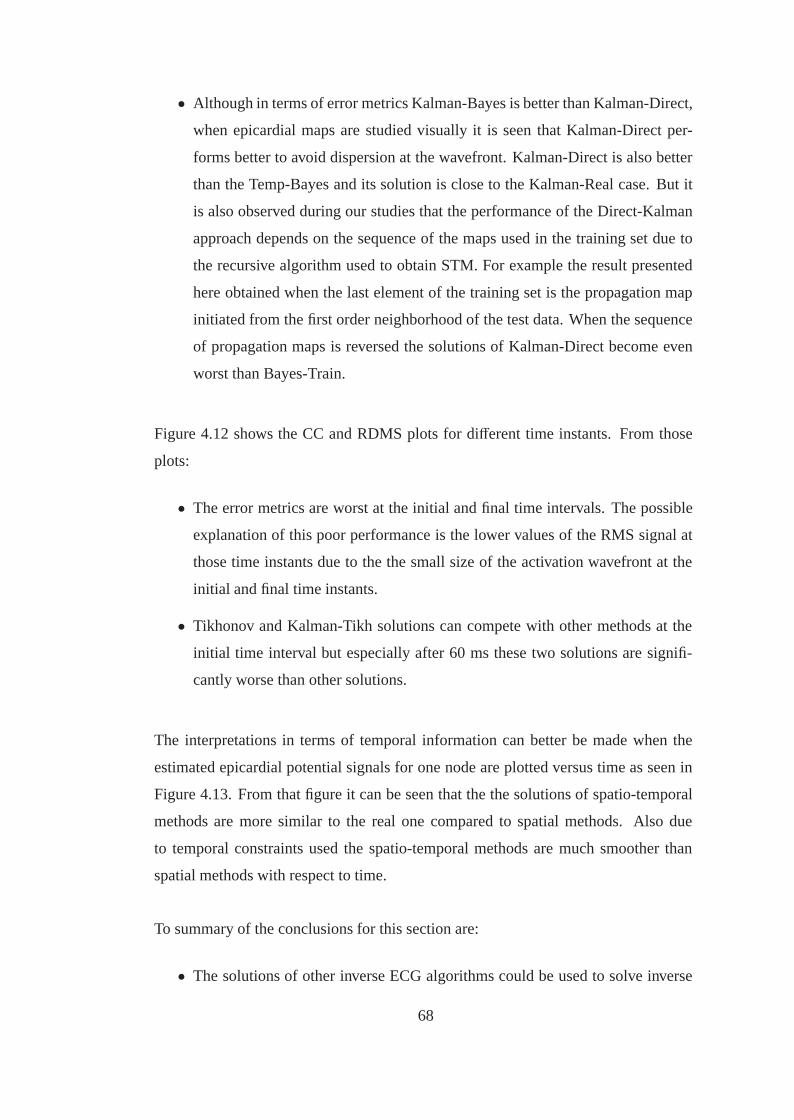
• Although in terms of error metrics Kalman-Bayes is better than Kalman-Direct,
when epicardial maps are studied visually it is seen that Kalman-Direct per-
forms better to avoid dispersion at the wavefront. Kalman-Direct is also better
than the Temp-Bayes and its solution is close to the Kalman-Real case. But it
is also observed during our studies that the performance of the Direct-Kalman
approach depends on the sequence of the maps used in the training set due to
the recursive algorithm used to obtain STM. For example the result presented
here obtained when the last element of the training set is the propagation map
initiated from the first order neighborhood of the test data. When the sequence
of propagation maps is reversed the solutions of Kalman-Direct become even
worst than Bayes-Train.
Figure 4.12 shows the CC and RDMS plots for different time instants. From those
plots:
• The error metrics are worst at the initial and final time intervals. The possible
explanation of this poor performance is the lower values of the RMS signal at
those time instants due to the the small size of the activation wavefront at the
initial and final time instants.
• Tikhonov and Kalman-Tikh solutions can compete with other methods at the
initial time interval but especially after 60 ms these two solutions are signifi-
cantly worse than other solutions.
The interpretations in terms of temporal information can better be made when the
estimated epicardial potential signals for one node are plotted versus time as seen in
Figure 4.13. From that figure it can be seen that the the solutions of spatio-temporal
methods are more similar to the real one compared to spatial methods. Also due
to temporal constraints used the spatio-temporal methods are much smoother than
spatial methods with respect to time.
To summary of the conclusions for this section are:
• The solutions of other inverse ECG algorithms could be used to solve inverse
68
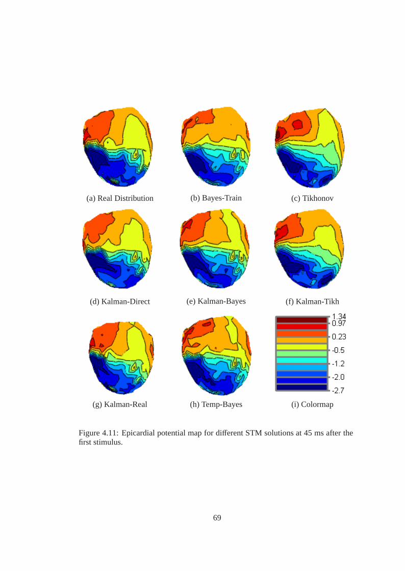
(a) Real Distribution (b) Bayes-Train (c) Tikhonov
(d) Kalman-Direct (e) Kalman-Bayes (f) Kalman-Tikh
(g) Kalman-Real (h) Temp-Bayes (i) Colormap
Figure 4.11: Epicardial potential map for different STM solutions at 45 ms after thefirst stimulus.
69

0 20 40 60 80 1000
0.1
0.2
0.3
0.4
0.5
0.6
0.7
0.8
0.9
1
time (ms)
CC
Correlation Coefficient vs Time
Bayes−TrainTikhonovTemp−BayesKalman−BayesKalman−TikhKalman−DirectKalman−Real
(a) The CC plot
0 20 40 60 80 1000
0.2
0.4
0.6
0.8
1
1.2
1.4
time (ms)
RD
MS
RDMS vs Time Plot
Bayes−TrainTikhonovTemp−BayesKalman−BayesKalman−TikhKalman−DirectKalman−Real
(b) The RDMS plot
Figure 4.12: The CC and RDMS values of different STM solutions with respect totime.
70
0 10 20 30 40 50 60 70 80 90 100−0.6
−0.4
−0.2
0
0.2
0.4
0.6
0.8
1
1.2
time (ms)
sign
al a
mpl
itude
(m
V)
The Electrogram for Epicardial Node 365
Real SignalBayes−TrainTikhonovTemp−BayesKalman−BayesKalman−TikhKalman−Direct
Figure 4.13: The real and estimated potential signal plot for the 365’th node on epi-cardium
71

problem of ECG with Kalman filter algorithm.
• This study is important in the sense that it shows the possible improvements
with the usage of spatio-temporal algorithms instead of spatial ones. Especially
the improvements obtained using Kalman-Bayes and Kalman-Tikh is important
because all a priori information used in those two techniques are obtained from
the spatial algorithm solutions.
• Kalman-Direct and Kalman-Bayes solutions performances are close to Kalman-
Real solution.
• Although Kalman-Direct seems to follow the wavefront very good its much
higher computational cost should also be considered. Also its dependence
on the sequence of elements in the training set considerably limits its usage.
Also the Kalman Direct performs worse than Kalman-Bayes, Kalman-Tikh and
Kalman-Real.
• Kalman-Bayes performs slightly better than Temp-Bayes but its computational
cost is higher. So if one can tolerate the extra computational time Kalman-
Bayes could be preferred instead of Temp-Bayes or Bayes-Train.
• The results of Kalman-Tikh are worse than Bayes-Train and its computational
time is higher but the advantage of Kalman-Tikh is that the necessity of using
training set could be avoided with that approach.
4.5 The Effects of Geometric Error in Cardiac Electrical Imaging and A Sta-
tistical Model to Overcome Those Errors: Enhanced Noise Model
In this section first the affects of geometric errors in cardiac electrical imaging for
the solutions obtained by Kalman Filter and Bayes-MAP will be studied. Then the
improvements obtained by modeling those geometric errors in a statistical sense will
be shown. According to this model geometric errors could be added to the inverse
solutions algorithms as independent and identically distributed Gaussian noise. The
new noise model is called the Enhanced noise model. The enhanced noise model is
firstly proposed by Kaipio et. al. and then used in optical tomography [76, 77]. To
72
the best of our knowledge this is the first application of this model to inverse ECG
problem.
4.5.1 Effects of Geometric Errors
The effects of the geometric errors were investigated by several studies [28, 62]. In
those studies the effects of geometric errors are shown to be more important (cause
more error in the constructed inverse solution) than errors in the conductivity values
within the thorax. For that reason the errors due to wrong conductivity assignments
are not covered in this thesis.
The forward calculations are same as in 4.4. But the inverse calculations differ in or-
der to simulate geometric errors. During the inverse calculations, position or the size
of heart mesh is changed in the model and a new transfer matrix is calculated with
this faulty mesh (F-mesh). Using this F-mesh in the inverse solution the geometric
errors that could occur in noninvasive ECG imaging applications are simulated. Two
kinds of geometric errors are investigated in this study. These are the wrong determi-
nation of heart’s position and size. These two problems could often occur due to the
movement of the heart. First, the consequences of the faulty determination of heart’s
location are examined. The error is created by shifting the heart from its original posi-
tion by 2 to 25 mm in the positive–x direction and using the transfer matrix calculated
from these F-meshes in the inverse solution. Next, wrong estimation of heart’s size is
examined. The error is created by multiplying the heart’s surface by a scalar varying
from 0.90 to 1.10 to adjust its size. For example if the heart’s surface is multiplied
by 0.95, 5 percent reduction in the heart’s size is achieved. These error margins are
enough because the modern techniques used today for geometry determination usu-
ally have smaller errors than those. The training set used here is same as in 4.4. The
simulation procedure for geometric errors is shown at Figure 4.14.
The inverse problem solution algorithms used here are:
1. Tikhonov: It is same as the one used at the previous section.
2. Kalman-Real: It uses the epicardial potential maps of the test data itself to
calculate STM.
73
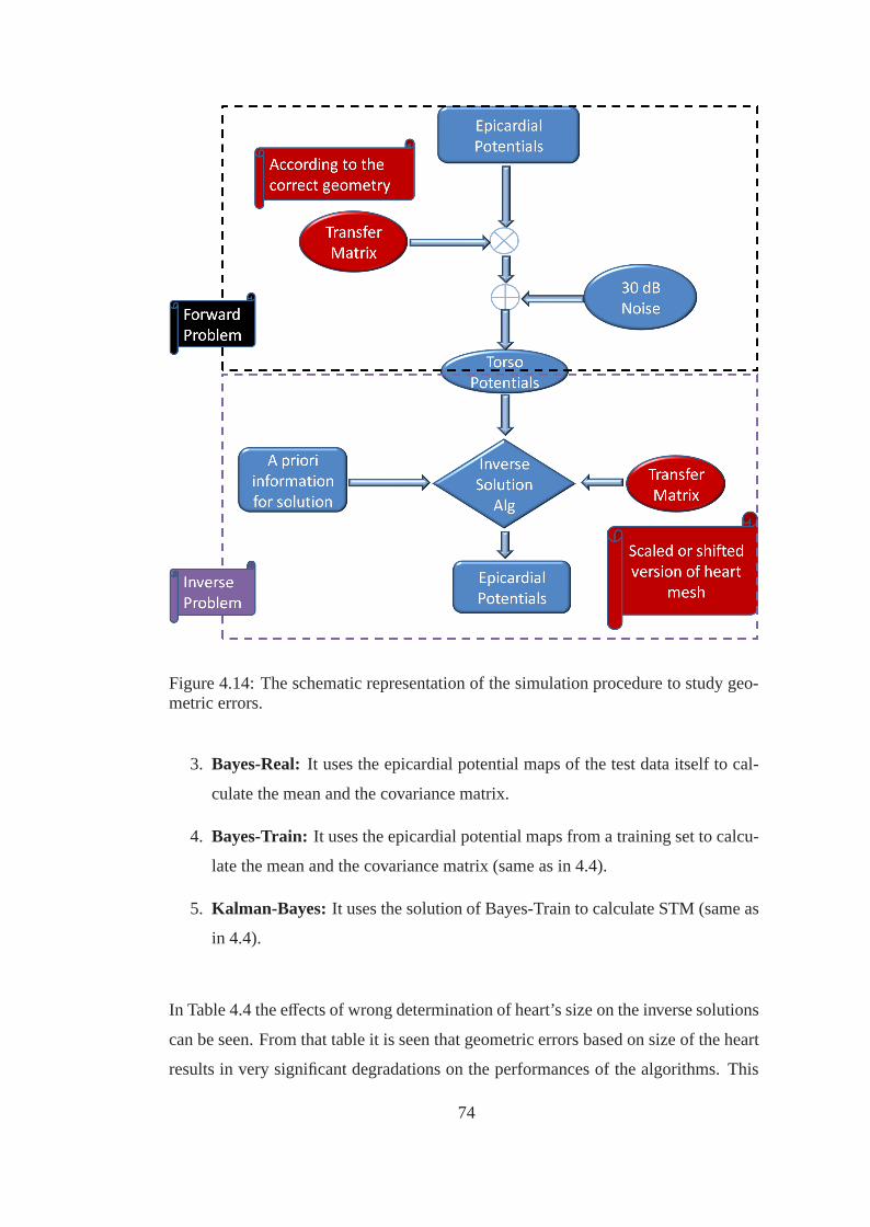
Figure 4.14: The schematic representation of the simulation procedure to study geo-metric errors.
3. Bayes-Real: It uses the epicardial potential maps of the test data itself to cal-
culate the mean and the covariance matrix.
4. Bayes-Train: It uses the epicardial potential maps from a training set to calcu-
late the mean and the covariance matrix (same as in 4.4).
5. Kalman-Bayes: It uses the solution of Bayes-Train to calculate STM (same as
in 4.4).
In Table 4.4 the effects of wrong determination of heart’s size on the inverse solutions
can be seen. From that table it is seen that geometric errors based on size of the heart
results in very significant degradations on the performances of the algorithms. This
74
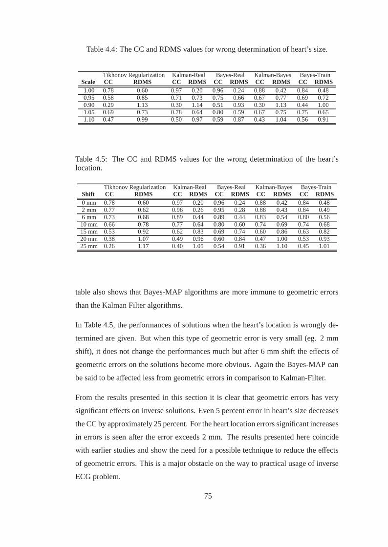
Table 4.4: The CC and RDMS values for wrong determination of heart’s size.
Tikhonov Regularization Kalman-Real Bayes-Real Kalman-Bayes Bayes-TrainScale CC RDMS CC RDMS CC RDMS CC RDMS CC RDMS1.00 0.78 0.60 0.97 0.20 0.96 0.24 0.88 0.42 0.84 0.480.95 0.58 0.85 0.71 0.73 0.75 0.66 0.67 0.77 0.69 0.720.90 0.29 1.13 0.30 1.14 0.51 0.93 0.30 1.13 0.44 1.001.05 0.69 0.73 0.78 0.64 0.80 0.59 0.67 0.75 0.75 0.651.10 0.47 0.99 0.50 0.97 0.59 0.87 0.43 1.04 0.56 0.91
Table 4.5: The CC and RDMS values for the wrong determination of the heart’slocation.
Tikhonov Regularization Kalman-Real Bayes-Real Kalman-Bayes Bayes-TrainShift CC RDMS CC RDMS CC RDMS CC RDMS CC RDMS0 mm 0.78 0.60 0.97 0.20 0.96 0.24 0.88 0.42 0.84 0.482 mm 0.77 0.62 0.96 0.26 0.95 0.28 0.88 0.43 0.84 0.496 mm 0.73 0.68 0.89 0.44 0.89 0.44 0.83 0.54 0.80 0.56
10 mm 0.66 0.78 0.77 0.64 0.80 0.60 0.74 0.69 0.74 0.6815 mm 0.53 0.92 0.62 0.83 0.69 0.74 0.60 0.86 0.63 0.8220 mm 0.38 1.07 0.49 0.96 0.60 0.84 0.47 1.00 0.53 0.9325 mm 0.26 1.17 0.40 1.05 0.54 0.91 0.36 1.10 0.45 1.01
table also shows that Bayes-MAP algorithms are more immune to geometric errors
than the Kalman Filter algorithms.
In Table 4.5, the performances of solutions when the heart’s location is wrongly de-
termined are given. But when this type of geometric error is very small (eg. 2 mm
shift), it does not change the performances much but after 6 mm shift the effects of
geometric errors on the solutions become more obvious. Again the Bayes-MAP can
be said to be affected less from geometric errors in comparison to Kalman-Filter.
From the results presented in this section it is clear that geometric errors has very
significant effects on inverse solutions. Even 5 percent error in heart’s size decreases
the CC by approximately 25 percent. For the heart location errors significant increases
in errors is seen after the error exceeds 2 mm. The results presented here coincide
with earlier studies and show the need for a possible technique to reduce the effects
of geometric errors. This is a major obstacle on the way to practical usage of inverse
ECG problem.
75
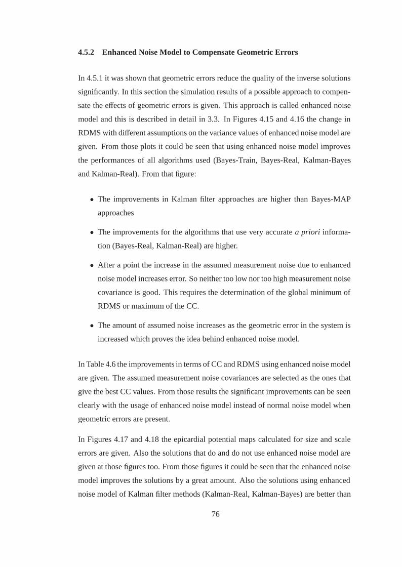
4.5.2 Enhanced Noise Model to Compensate Geometric Errors
In 4.5.1 it was shown that geometric errors reduce the quality of the inverse solutions
significantly. In this section the simulation results of a possible approach to compen-
sate the effects of geometric errors is given. This approach is called enhanced noise
model and this is described in detail in 3.3. In Figures 4.15 and 4.16 the change in
RDMS with different assumptions on the variance values of enhanced noise model are
given. From those plots it could be seen that using enhanced noise model improves
the performances of all algorithms used (Bayes-Train, Bayes-Real, Kalman-Bayes
and Kalman-Real). From that figure:
• The improvements in Kalman filter approaches are higher than Bayes-MAP
approaches
• The improvements for the algorithms that use very accurate a priori informa-
tion (Bayes-Real, Kalman-Real) are higher.
• After a point the increase in the assumed measurement noise due to enhanced
noise model increases error. So neither too low nor too high measurement noise
covariance is good. This requires the determination of the global minimum of
RDMS or maximum of the CC.
• The amount of assumed noise increases as the geometric error in the system is
increased which proves the idea behind enhanced noise model.
In Table 4.6 the improvements in terms of CC and RDMS using enhanced noise model
are given. The assumed measurement noise covariances are selected as the ones that
give the best CC values. From those results the significant improvements can be seen
clearly with the usage of enhanced noise model instead of normal noise model when
geometric errors are present.
In Figures 4.17 and 4.18 the epicardial potential maps calculated for size and scale
errors are given. Also the solutions that do and do not use enhanced noise model are
given at those figures too. From those figures it could be seen that the enhanced noise
model improves the solutions by a great amount. Also the solutions using enhanced
noise model of Kalman filter methods (Kalman-Real, Kalman-Bayes) are better than
76
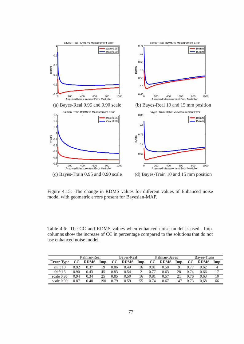
0 200 400 600 800 10000.5
0.6
0.7
0.8
0.9
1
Assumed Measurement Error Multiplier
RD
MS
Bayes−Real RDMS vs Mesaurement Error
scale 0.95scale 0.90
(a) Bayes-Real 0.95 and 0.90 scale
0 200 400 600 800 10000.45
0.5
0.55
0.6
0.65
0.7
0.75
Assumed Measurement Error Multiplier
RD
MS
Bayes−Real RDMS vs Mesaurement Error
10 mm15 mm
(b) Bayes-Real 10 and 15 mm position
0 200 400 600 800 10000.5
0.6
0.7
0.8
0.9
1
1.1
1.2
1.3
Assumed Measurement Error Multiplier
RD
MS
Kalman−Train RDMS vs Mesaurement Error
scale 0.95scale 0.90
(c) Bayes-Train 0.95 and 0.90 scale
0 200 400 600 800 1000
0.65
0.7
0.75
0.8
0.85
Assumed Measurement Error Multiplier
RD
MS
Bayes−Train RDMS vs Mesaurement Error
10 mm15 mm
(d) Bayes-Train 10 and 15 mm position
Figure 4.15: The change in RDMS values for different values of Enhanced noisemodel with geometric errors present for Bayesian-MAP.
Table 4.6: The CC and RDMS values when enhanced noise model is used. Imp.columns show the increase of CC in percentage compared to the solutions that do notuse enhanced noise model.
Kalman-Real Bayes-Real Kalman-Bayes Bayes-TrainError Type CC RDMS Imp. CC RDMS Imp. CC RDMS Imp. CC RDMS Imp.
shift 10 0.92 0.37 19 0.86 0.49 16 0.81 0.58 9 0.77 0.62 4shift 15 0.90 0.43 45 0.83 0.54 2 0.77 0.63 28 0.74 0.66 17
scale 0.95 0.94 0.34 25 0.85 0.50 16 0.81 0.57 21 0.76 0.63 10scale 0.90 0.87 0.48 190 0.79 0.59 55 0.74 0.67 147 0.73 0,68 66
77
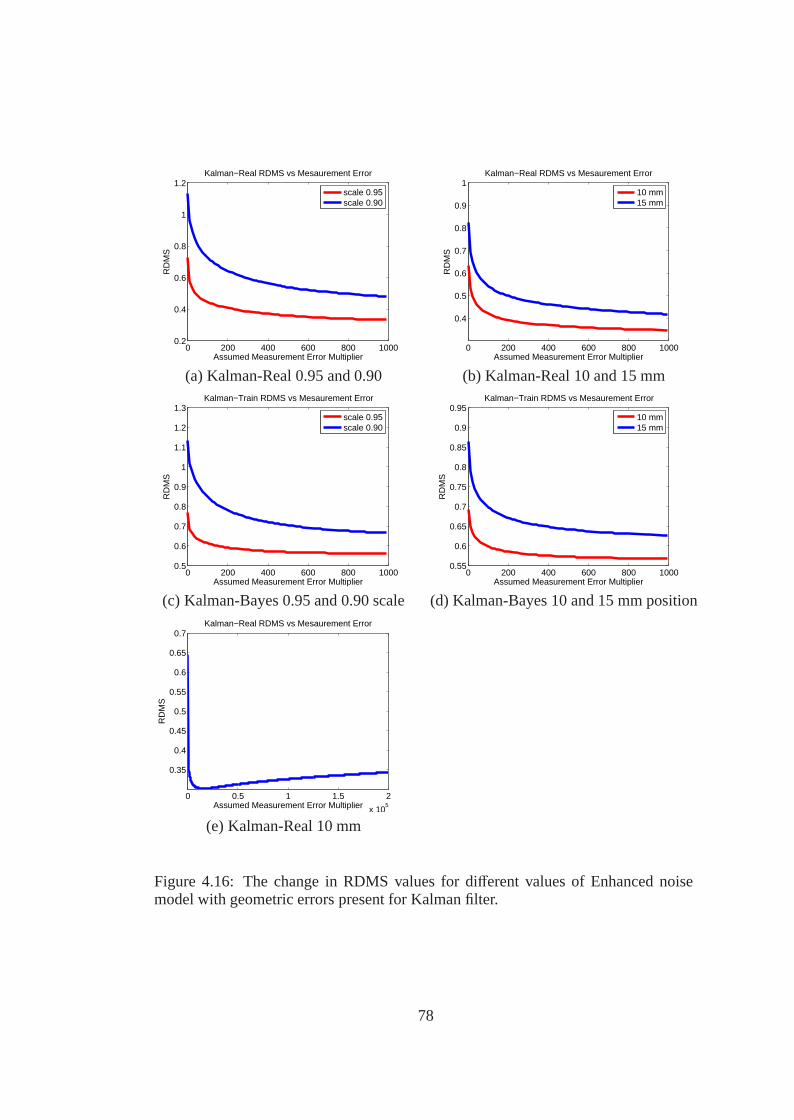
0 200 400 600 800 10000.2
0.4
0.6
0.8
1
1.2
Assumed Measurement Error Multiplier
RD
MS
Kalman−Real RDMS vs Mesaurement Error
scale 0.95scale 0.90
(a) Kalman-Real 0.95 and 0.90
0 200 400 600 800 1000
0.4
0.5
0.6
0.7
0.8
0.9
1
Assumed Measurement Error Multiplier
RD
MS
Kalman−Real RDMS vs Mesaurement Error
10 mm15 mm
(b) Kalman-Real 10 and 15 mm
0 200 400 600 800 10000.5
0.6
0.7
0.8
0.9
1
1.1
1.2
1.3
Assumed Measurement Error Multiplier
RD
MS
Kalman−Train RDMS vs Mesaurement Error
scale 0.95scale 0.90
(c) Kalman-Bayes 0.95 and 0.90 scale
0 200 400 600 800 10000.55
0.6
0.65
0.7
0.75
0.8
0.85
0.9
0.95
Assumed Measurement Error Multiplier
RD
MS
Kalman−Train RDMS vs Mesaurement Error
10 mm15 mm
(d) Kalman-Bayes 10 and 15 mm position
0 0.5 1 1.5 2
x 105
0.35
0.4
0.45
0.5
0.55
0.6
0.65
0.7
Assumed Measurement Error Multiplier
RD
MS
Kalman−Real RDMS vs Mesaurement Error
(e) Kalman-Real 10 mm
Figure 4.16: The change in RDMS values for different values of Enhanced noisemodel with geometric errors present for Kalman filter.
78
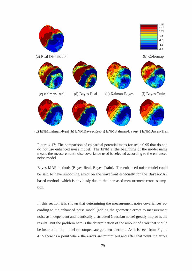
(a) Real Distribution (b) Colormap
(c) Kalman-Real (d) Bayes-Real (e) Kalman-Bayes (f) Bayes-Train
(g) ENMKalman-Real (h) ENMBayes-Real(i) ENMKalman-Bayes(j) ENMBayes-Train
Figure 4.17: The comparison of epicardial potential maps for scale 0.95 that do anddo not use enhanced noise model. The ENM at the beginning of the model namemeans the measurement noise covariance used is selected according to the enhancednoise model.
Bayes-MAP methods (Bayes-Real, Bayes-Train). The enhanced noise model could
be said to have smoothing affect on the wavefront especially for the Bayes-MAP
based methods which is obviously due to the increased measurement error assump-
tion.
In this section it is shown that determining the measurement noise covariances ac-
cording to the enhanced noise model (adding the geometric errors to measurement
noise as independent and identically distributed Gaussian noise) greatly improves the
results. But the problem here is the determination of the amount of error that should
be inserted to the model to compensate geometric errors. As it is seen from Figure
4.15 there is a point where the errors are minimized and after that point the errors
79
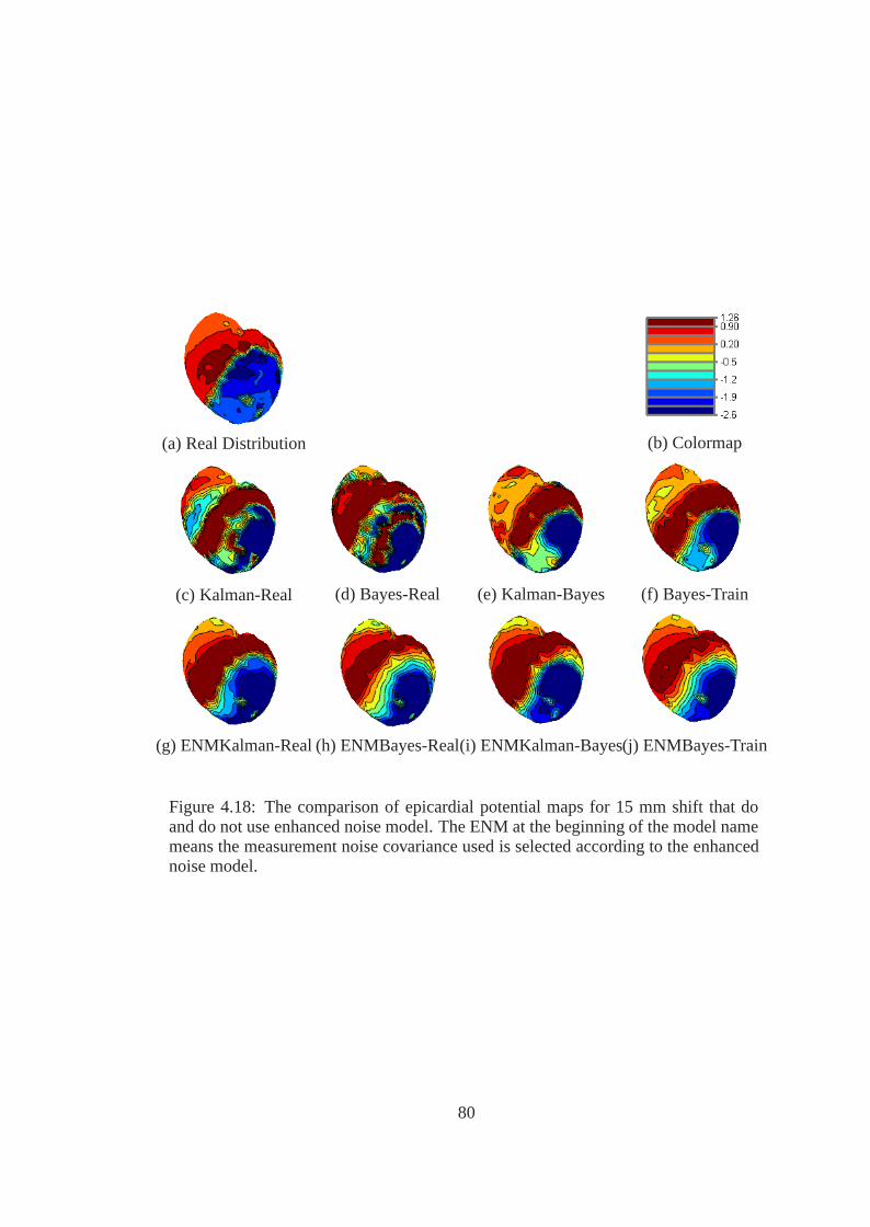
(a) Real Distribution (b) Colormap
(c) Kalman-Real (d) Bayes-Real (e) Kalman-Bayes (f) Bayes-Train
(g) ENMKalman-Real (h) ENMBayes-Real(i) ENMKalman-Bayes(j) ENMBayes-Train
Figure 4.18: The comparison of epicardial potential maps for 15 mm shift that doand do not use enhanced noise model. The ENM at the beginning of the model namemeans the measurement noise covariance used is selected according to the enhancednoise model.
80

starts to increase again. Another important observation is the error decline at the
Kalman filter algorithms are a lot more comparison to Bayes-MAP algorithms when
enhanced noise model is used.
4.6 Determination of the Measurement and Process Noise Covariance Matrices
Using Residuals
In this section the measurement and process noise covariance matrices are estimated
using a method based on residuals. In order to test the performance of the methods
different scenarios are employed. In the first scenario both measurement and process
noise covariance matrices are calculated for the case that no geometric error exists
and only independent and identically distributed (iid) 15 or 30 dB noise is present.
By doing so the algorithm’s ability to compensate additive errors is tested. In the
second scenario again both process and measurement noise covariance matrices are
calculated but this time along with 30dB iid noise also geometric errors are present
at the system. This scenario is implemented to find out if residual based algorithm
is able to compensate the geometric errors. In the third and fourth scenarios only
measurement noise covariance matrix is calculated and the value that gives highest
CC value for 30 dB noise case is used as process noise covariance. The difference
between third and fourth scenarios is that the third scenario is simulated for 15 and 30
dB iid noise cases and the fourth scenario is tested for the case when both geometric
errors and 30 dB noise are present. As stated in 4.5.2 the determination of correct
values for the process noise covariance without using CC and RDMS is the most
important problem that needs to be solved before the usage of ENM in practical cases.
The fourth scenario at this section refers to that problem and tries to determine the
measurement noise covariance matrix that should be used in the system to compensate
geometric errors by using body surface potentials
At the first scenario the process and measurement noise covariances are estimated
for the cases where 30 dB or 15 dB independent and identically distributed Gaussian
noise is added to the system. The results for this scenario are given in Table 4.7. From
that table:
81
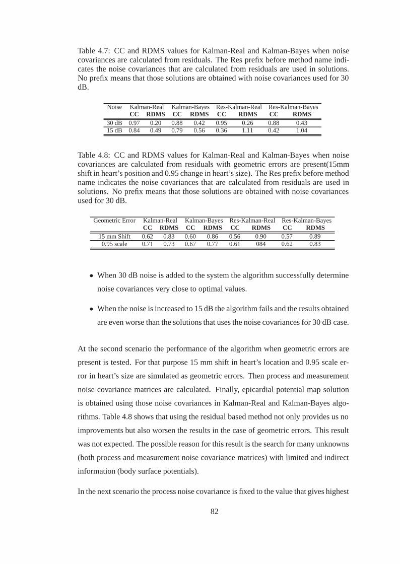
Table 4.7: CC and RDMS values for Kalman-Real and Kalman-Bayes when noisecovariances are calculated from residuals. The Res prefix before method name indi-cates the noise covariances that are calculated from residuals are used in solutions.No prefix means that those solutions are obtained with noise covariances used for 30dB.
Noise Kalman-Real Kalman-Bayes Res-Kalman-Real Res-Kalman-BayesCC RDMS CC RDMS CC RDMS CC RDMS
30 dB 0.97 0.20 0.88 0.42 0.95 0.26 0.88 0.4315 dB 0.84 0.49 0.79 0.56 0.36 1.11 0.42 1.04
Table 4.8: CC and RDMS values for Kalman-Real and Kalman-Bayes when noisecovariances are calculated from residuals with geometric errors are present(15mmshift in heart’s position and 0.95 change in heart’s size). The Res prefix before methodname indicates the noise covariances that are calculated from residuals are used insolutions. No prefix means that those solutions are obtained with noise covariancesused for 30 dB.
Geometric Error Kalman-Real Kalman-Bayes Res-Kalman-Real Res-Kalman-BayesCC RDMS CC RDMS CC RDMS CC RDMS
15 mm Shift 0.62 0.83 0.60 0.86 0.56 0.90 0.57 0.890.95 scale 0.71 0.73 0.67 0.77 0.61 084 0.62 0.83
• When 30 dB noise is added to the system the algorithm successfully determine
noise covariances very close to optimal values.
• When the noise is increased to 15 dB the algorithm fails and the results obtained
are even worse than the solutions that uses the noise covariances for 30 dB case.
At the second scenario the performance of the algorithm when geometric errors are
present is tested. For that purpose 15 mm shift in heart’s location and 0.95 scale er-
ror in heart’s size are simulated as geometric errors. Then process and measurement
noise covariance matrices are calculated. Finally, epicardial potential map solution
is obtained using those noise covariances in Kalman-Real and Kalman-Bayes algo-
rithms. Table 4.8 shows that using the residual based method not only provides us no
improvements but also worsen the results in the case of geometric errors. This result
was not expected. The possible reason for this result is the search for many unknowns
(both process and measurement noise covariance matrices) with limited and indirect
information (body surface potentials).
In the next scenario the process noise covariance is fixed to the value that gives highest
82
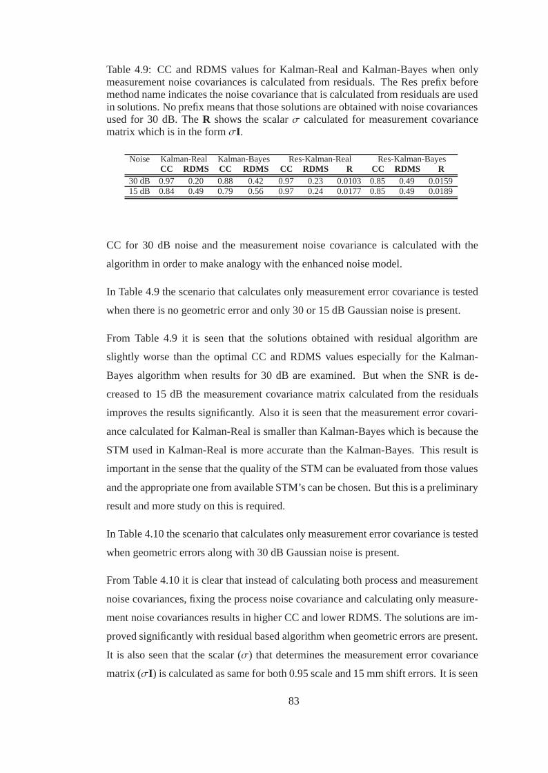
Table 4.9: CC and RDMS values for Kalman-Real and Kalman-Bayes when onlymeasurement noise covariances is calculated from residuals. The Res prefix beforemethod name indicates the noise covariance that is calculated from residuals are usedin solutions. No prefix means that those solutions are obtained with noise covariancesused for 30 dB. The R shows the scalar σ calculated for measurement covariancematrix which is in the form σI.
Noise Kalman-Real Kalman-Bayes Res-Kalman-Real Res-Kalman-BayesCC RDMS CC RDMS CC RDMS R CC RDMS R
30 dB 0.97 0.20 0.88 0.42 0.97 0.23 0.0103 0.85 0.49 0.015915 dB 0.84 0.49 0.79 0.56 0.97 0.24 0.0177 0.85 0.49 0.0189
CC for 30 dB noise and the measurement noise covariance is calculated with the
algorithm in order to make analogy with the enhanced noise model.
In Table 4.9 the scenario that calculates only measurement error covariance is tested
when there is no geometric error and only 30 or 15 dB Gaussian noise is present.
From Table 4.9 it is seen that the solutions obtained with residual algorithm are
slightly worse than the optimal CC and RDMS values especially for the Kalman-
Bayes algorithm when results for 30 dB are examined. But when the SNR is de-
creased to 15 dB the measurement covariance matrix calculated from the residuals
improves the results significantly. Also it is seen that the measurement error covari-
ance calculated for Kalman-Real is smaller than Kalman-Bayes which is because the
STM used in Kalman-Real is more accurate than the Kalman-Bayes. This result is
important in the sense that the quality of the STM can be evaluated from those values
and the appropriate one from available STM’s can be chosen. But this is a preliminary
result and more study on this is required.
In Table 4.10 the scenario that calculates only measurement error covariance is tested
when geometric errors along with 30 dB Gaussian noise is present.
From Table 4.10 it is clear that instead of calculating both process and measurement
noise covariances, fixing the process noise covariance and calculating only measure-
ment noise covariances results in higher CC and lower RDMS. The solutions are im-
proved significantly with residual based algorithm when geometric errors are present.
It is also seen that the scalar (σ) that determines the measurement error covariance
matrix (σI) is calculated as same for both 0.95 scale and 15 mm shift errors. It is seen
83
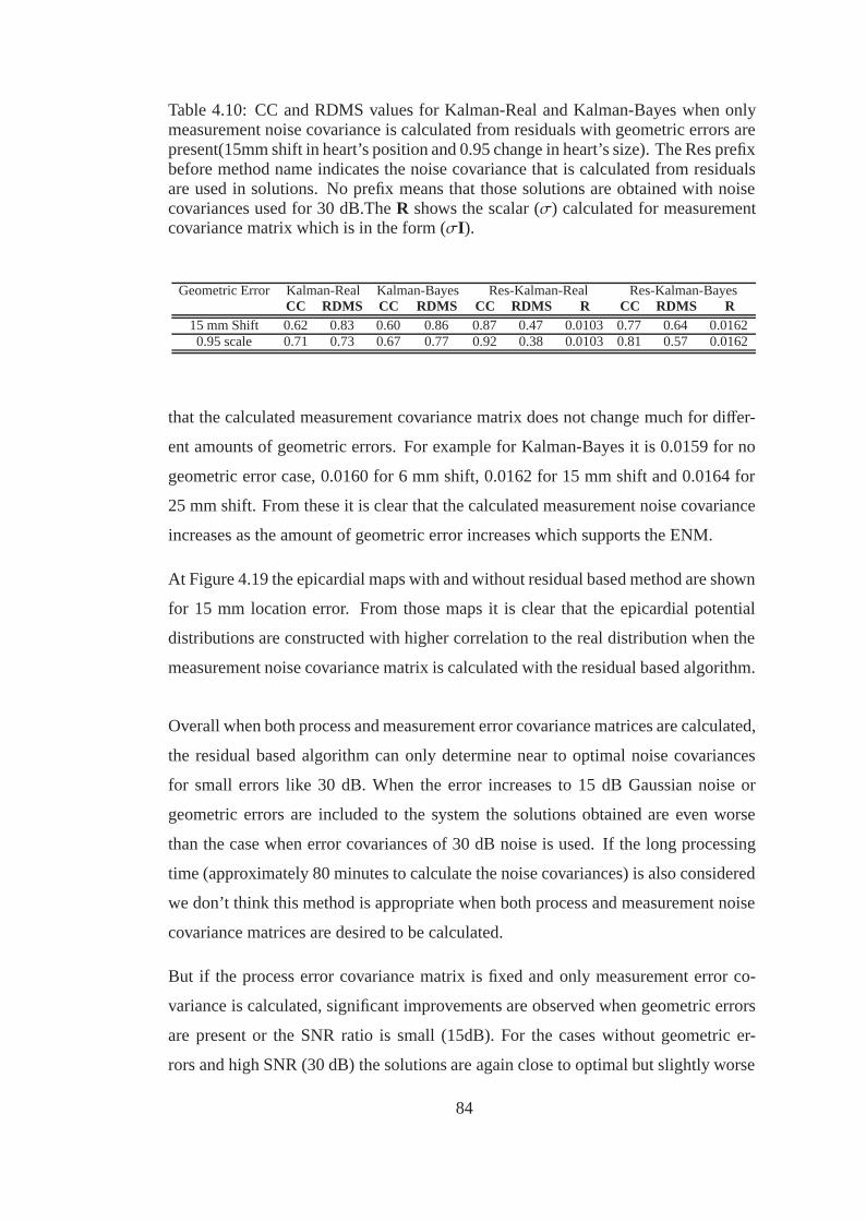
Table 4.10: CC and RDMS values for Kalman-Real and Kalman-Bayes when onlymeasurement noise covariance is calculated from residuals with geometric errors arepresent(15mm shift in heart’s position and 0.95 change in heart’s size). The Res prefixbefore method name indicates the noise covariance that is calculated from residualsare used in solutions. No prefix means that those solutions are obtained with noisecovariances used for 30 dB.The R shows the scalar (σ) calculated for measurementcovariance matrix which is in the form (σI).
Geometric Error Kalman-Real Kalman-Bayes Res-Kalman-Real Res-Kalman-BayesCC RDMS CC RDMS CC RDMS R CC RDMS R
15 mm Shift 0.62 0.83 0.60 0.86 0.87 0.47 0.0103 0.77 0.64 0.01620.95 scale 0.71 0.73 0.67 0.77 0.92 0.38 0.0103 0.81 0.57 0.0162
that the calculated measurement covariance matrix does not change much for differ-
ent amounts of geometric errors. For example for Kalman-Bayes it is 0.0159 for no
geometric error case, 0.0160 for 6 mm shift, 0.0162 for 15 mm shift and 0.0164 for
25 mm shift. From these it is clear that the calculated measurement noise covariance
increases as the amount of geometric error increases which supports the ENM.
At Figure 4.19 the epicardial maps with and without residual based method are shown
for 15 mm location error. From those maps it is clear that the epicardial potential
distributions are constructed with higher correlation to the real distribution when the
measurement noise covariance matrix is calculated with the residual based algorithm.
Overall when both process and measurement error covariance matrices are calculated,
the residual based algorithm can only determine near to optimal noise covariances
for small errors like 30 dB. When the error increases to 15 dB Gaussian noise or
geometric errors are included to the system the solutions obtained are even worse
than the case when error covariances of 30 dB noise is used. If the long processing
time (approximately 80 minutes to calculate the noise covariances) is also considered
we don’t think this method is appropriate when both process and measurement noise
covariance matrices are desired to be calculated.
But if the process error covariance matrix is fixed and only measurement error co-
variance is calculated, significant improvements are observed when geometric errors
are present or the SNR ratio is small (15dB). For the cases without geometric er-
rors and high SNR (30 dB) the solutions are again close to optimal but slightly worse
84

(a) Real Distribution (b) Kalman-Real (c) Kalman-Bayes
(d) Colormap (e) Res-Kalman-Real (f) Res-Kalman-Bayes
Figure 4.19: Epicardial potential maps for 54 ms after the first stimulus. The mapsolutions of both Kalman-Real and Kalman-Bayes are given when 15 mm shift geo-metric error is present. The Res prefix before the name of the method stands for themeasurement noise covariance is calculated with the residual based algorithm. Whenthere is no prefix it means that the same noise covariance matrices as the case in 30dB Gaussian noise are used.
especially for Kalman-Bayes algorithm. We think the significant improvements in ge-
ometric error cases are more important than the slight decreases in error performance
for the cases without geometric errors and this algorithm can be used for inverse ECG
problem. But here again a major disadvantage should be noted which is the long
processing time which is approximately 60 minutes. Another promising result is that
the measurement noise covariance calculated for Kalman-Bayes is higher than the
Kalman-Real. The reason for this increase is due to the quality of the STM used in
algorithms. This result should be further studied and it could be used as an indicator
of the quality of the STM used in Kalman filter.
4.7 Expectation Maximization Algorithm to Determine Measurement and Pro-
cess Noise Covariance Matrices
As described before the values of measurement and process noise covariances are also
critical in order to obtain good solutions. At this section expectation maximization
85

algorithm is used to determine those covariances.
The first scenario used is for the case of additive white Gaussian noise. For that
purpose body surface potentials are simulated from the epicardial potentials, at 15
or 30 dB SNR. Then from those BSP’s the epicardial potentials are estimated using
Kalman-Real and Kalman-Bayes approaches. The initial error covariances needed
for EM algorithm are chosen randomly as 0.01xIN for process and 0.16xIM for mea-
surement noise where IN is the NxN and IM is the MxM identity matrices. Here N is
the number of epicardial nodes and M is the number of BSP measurement electrodes.
In Figure 4.20 the RDMS versus iteration number plots are shown. From those plots
it is seen that the EM algorithm is able to determine the correct values for noise co-
variances for both 15dB and 30 dB Gaussian noise cases. Also the algorithm achieves
to find the covariances not only for Kalman-Real case both also for Kalman-Bayes
which is important because the usage of Kalman-Real is not possible for practical
cases. Another important fact is no significant improvement is observed in terms of
RDMS values after the first five iterations which means that epicardial potential esti-
mations could be obtained just after five iterations. Because each iteration takes about
65 seconds it is wise to avoid unnecessary iterations.
In the second scenario only the measurement error covariance matrix is calculated
to compensate the effects of geometric errors. For that purpose the process noise
covariance is fixed and only the measurement noise covariance is updated with EM.
The initial process and measurement noise covariance matrices are the ones that give
the best CC values when no geometric error is present. Only the measurement noise
covariance is updated at this scenario to make an analogy with the enhanced noise
model described before where the geometric errors are compensated with the increase
in the measurement error covariance. In Figure 4.21 RDMS versus iteration plots for
the geometric errors 15 mm shift and 0.95 scale are given for the Kalman-Real and
Kalman Bayes algorithms. The inferences from those plots are:
• Very significant improvements are obtained in terms of error metrics.
• The convergence is completed usually at five iterations.
• The global minimum point sought for ENM is found with EM algorithm from
86
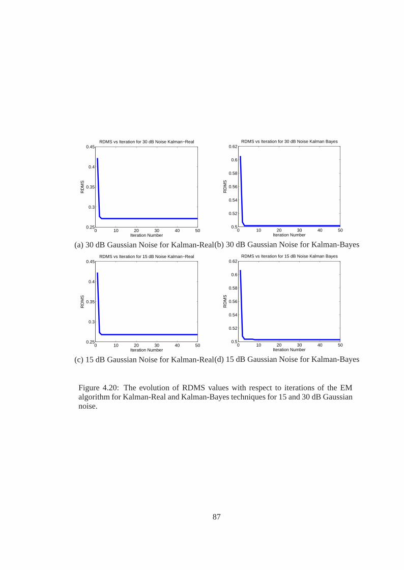
0 10 20 30 40 500.25
0.3
0.35
0.4
0.45RDMS vs Iteration for 30 dB Noise Kalman−Real
Iteration Number
RD
MS
(a) 30 dB Gaussian Noise for Kalman-Real
0 10 20 30 40 500.5
0.52
0.54
0.56
0.58
0.6
0.62RDMS vs Iteration for 30 dB Noise Kalman Bayes
Iteration Number
RD
MS
(b) 30 dB Gaussian Noise for Kalman-Bayes
0 10 20 30 40 500.25
0.3
0.35
0.4
0.45RDMS vs Iteration for 15 dB Noise Kalman−Real
Iteration Number
RD
MS
(c) 15 dB Gaussian Noise for Kalman-Real
0 10 20 30 40 500.5
0.52
0.54
0.56
0.58
0.6
0.62RDMS vs Iteration for 15 dB Noise Kalman Bayes
Iteration Number
RD
MS
(d) 15 dB Gaussian Noise for Kalman-Bayes
Figure 4.20: The evolution of RDMS values with respect to iterations of the EMalgorithm for Kalman-Real and Kalman-Bayes techniques for 15 and 30 dB Gaussiannoise.
87

the body surface potentials and this is a very important result to compensate
geometric errors.
In the last scenario both the measurement and process noise covariances are updated
with EM algorithm for the case where the geometric errors are present. As in the
second scenario the initial process and measurement noise covariance matrices are
selected as the ones that give the best CC values when no geometric error is present
and the geometric errors simulated are the 15 mm shift and 0.95 scale. This time
as seen from Figure 4.22 again improvements are obtained but unlike the first and
second scenarios the RDMS values decrease slowly which requires more iterations.
Another observation from those plots is that the improvements in the Kalman-Real
algorithm is higher than those in Kalman-Bayes algorithm, which is due to the quality
of the a priori information. This result was also observed with the ENM.
The epicardial potential maps for the cases explained in scenario one are given in
Figures 4.23. For the second and third scenarios the results are shown in Figure
4.24 and 4.25. The epicardial potentials maps also support our earlier inferences and
improvements using EM algorithm are obvious.
In this section the EM algorithm is used to calculate the process and measurement
noise covariances. The overall results obtained with EM studies are:
• For 15 and 30 dB Gaussian noise cases only five iterations with the EM algo-
rithm is enough to calculate the optimal noise covariances.
• For the case of geometric errors when only measurement noise covariance is
updated with EM, the results are improved significantly with EM algorithm.
This result also supports the assumption made at the enhanced noise model.
• For the case of geometric errors when both measurement and process noise co-
variances are updated by EM, the improvements are smaller than those obtained
when only the measurement noise covariance matrix is updated by EM. Also
the convergence rate is much slower than first and second scenarios (it still
converges after 500 iterations). The possible reason for smaller convergence
88
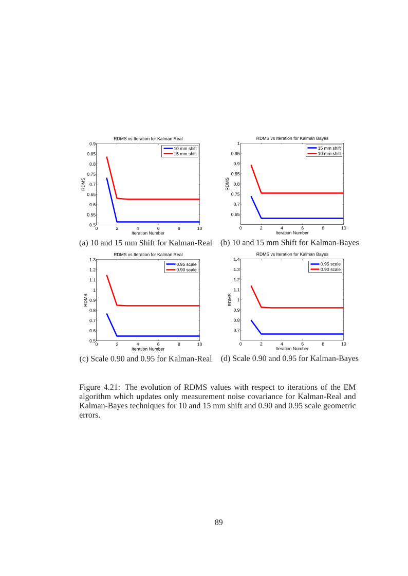
0 2 4 6 8 100.5
0.55
0.6
0.65
0.7
0.75
0.8
0.85
0.9RDMS vs Iteration for Kalman Real
Iteration Number
RD
MS
10 mm shift15 mm shift
(a) 10 and 15 mm Shift for Kalman-Real
0 2 4 6 8 10
0.65
0.7
0.75
0.8
0.85
0.9
0.95
1RDMS vs Iteration for Kalman Bayes
Iteration NumberR
DM
S
15 mm shift10 mm shift
(b) 10 and 15 mm Shift for Kalman-Bayes
0 2 4 6 8 100.5
0.6
0.7
0.8
0.9
1
1.1
1.2
1.3RDMS vs Iteration for Kalman Real
Iteration Number
RD
MS
0.95 scale0.90 scale
(c) Scale 0.90 and 0.95 for Kalman-Real
0 2 4 6 8 10
0.7
0.8
0.9
1
1.1
1.2
1.3
1.4RDMS vs Iteration for Kalman Bayes
Iteration Number
RD
MS
0.95 scale0.90 scale
(d) Scale 0.90 and 0.95 for Kalman-Bayes
Figure 4.21: The evolution of RDMS values with respect to iterations of the EMalgorithm which updates only measurement noise covariance for Kalman-Real andKalman-Bayes techniques for 10 and 15 mm shift and 0.90 and 0.95 scale geometricerrors.
89

0 100 200 300 400 5000.7
0.72
0.74
0.76
0.78
0.8
0.82RDMS vs Iteration for 15 mm Shift Noise Kalman−Real
Iteration Number
RD
MS
(a) 15 mm Shift for Kalman-Real
0 100 200 300 400 5000.82
0.83
0.84
0.85
0.86
0.87
0.88
0.89
0.9RDMS vs Iteration for 15 mm Shift Noise Kalman Bayes
Iteration Number
RD
MS
(b) 15 mm Shift for Kalman-Bayes
0 100 200 300 400 5000.6
0.62
0.64
0.66
0.68
0.7
0.72RDMS vs Iteration for Scale:095 Noise Kalman−Real
Iteration Number
RD
MS
(c) Scale 0.95 for Kalman-Real
0 100 200 300 400 5000.72
0.73
0.74
0.75
0.76
0.77
0.78
0.79
0.8RDMS vs Iteration for Scale:095 Noise Kalman Bayes
Iteration Number
RD
MS
(d) Scale 0.95 for Kalman-Bayes
Figure 4.22: The evolution of RDMS values with respect to iterations of the EMalgorithm for Kalman-Real and Kalman-Bayes techniques for 15 mm shift and 0.95scale geometric errors.
90

is because determining the optimal values for both measurement and process
noise covariances is a lot more complex than determining only the measure-
ment noise covariance.
91
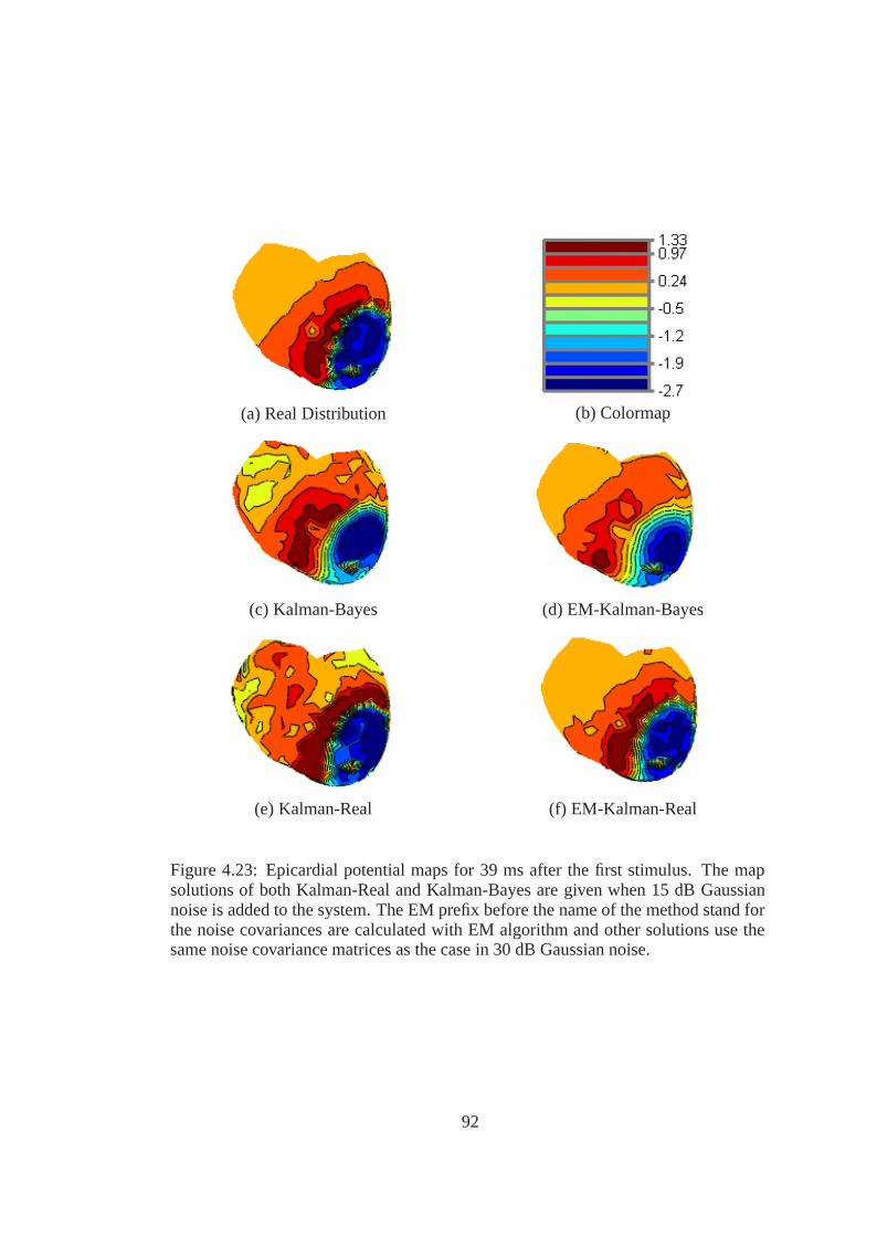
(a) Real Distribution (b) Colormap
(c) Kalman-Bayes (d) EM-Kalman-Bayes
(e) Kalman-Real (f) EM-Kalman-Real
Figure 4.23: Epicardial potential maps for 39 ms after the first stimulus. The mapsolutions of both Kalman-Real and Kalman-Bayes are given when 15 dB Gaussiannoise is added to the system. The EM prefix before the name of the method stand forthe noise covariances are calculated with EM algorithm and other solutions use thesame noise covariance matrices as the case in 30 dB Gaussian noise.
92

(a) Real Distribution (b) Colormap
(c) Kalman-Bayes (d) EM-Kalman-Bayes (e) EM-Kalman-Bayes only R
(f) Kalman-Real (g) EM-Kalman-Real (h) EM-Kalman-Real only R
Figure 4.24: Epicardial potential maps for 39 ms after the first stimulus. The mapsolutions of both Kalman-Real and Kalman-Bayes are given when 15 mm shift geo-metric error is present. The EM prefix before the name of the method stands for bothmeasurement and process noise covariances are calculated with EM algorithm. ’onlyR’ means only the measurement error is updated and when there is no prefix it meansthat the same noise covariance matrices as the case in 30 dB Gaussian noise are used.
93
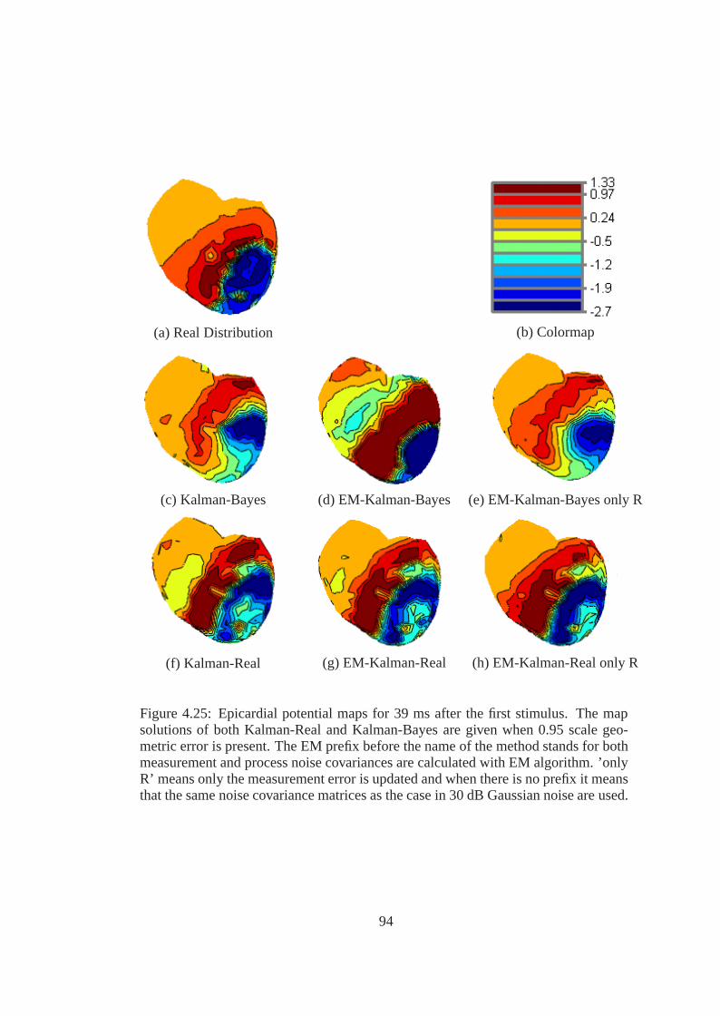
(a) Real Distribution (b) Colormap
(c) Kalman-Bayes (d) EM-Kalman-Bayes (e) EM-Kalman-Bayes only R
(f) Kalman-Real (g) EM-Kalman-Real (h) EM-Kalman-Real only R
Figure 4.25: Epicardial potential maps for 39 ms after the first stimulus. The mapsolutions of both Kalman-Real and Kalman-Bayes are given when 0.95 scale geo-metric error is present. The EM prefix before the name of the method stands for bothmeasurement and process noise covariances are calculated with EM algorithm. ’onlyR’ means only the measurement error is updated and when there is no prefix it meansthat the same noise covariance matrices as the case in 30 dB Gaussian noise are used.
94
CHAPTER 5
CONCLUSIONS
This thesis focuses on three major problems. The first one is the solution of inverse
problem of ECG using spatio-temporal methods especially with Kalman filter. The
second study is on the effects of geometric errors and a noise model to include geo-
metric noise to the general formulation. The last study focuses on the determination
of process and measurement noise covariances using body surface potentials with and
without geometric errors. The inverse solution scenarios used in those three studies
are
1. Tikhonov: The zero’th order Tikhonov regularization solution in which a dif-
ferent regularization parameter was calculated using the L-Curve approach for
each time instant.
2. Kalman-Tikh: The solution of the zero’th order Tikhonov regularization was
used to calculate the STM.
3. Bayes-Real: The epicardial potential maps of the test data itself are used to
calculate the mean and the covariance matrix in the spatial Bayesian MAP es-
timation.
4. Kalman-Real: The epicardial potential maps of the test data itself were used
to calculate the STM.
5. Bayes-Train: The epicardial potential maps from a training set were used to
calculate the mean and the covariance matrix in the spatial Bayesian MAP es-
timation.
95
6. Temp-Bayes: The spatio-temporal Bayesian MAP solution with a priori infor-
mation from the training set.
7. Kalman-Bayes: A training set was used to obtain the solution using the spatial
Bayesian MAP (Bayes-Train) and then this solution was used to calculate the
STM.
8. Kalman-Direct: A training set was used to calculate the STM directly.
5.1 Spatio-temporal Methods for Inverse Problem of ECG
In this work, Tikhonov, Kalman-Tikh, Bayes-Train, Kalman-Bayes, Temp-Bayes and
Kalman-Direct approaches were compared. But before the comparisons could be
made, one of the major difficulties for the solution of inverse problem of ECG us-
ing the Kalman filter approach had to be solved. This difficulty was the determi-
nation of the state transition matrix (STM) which models the temporal evolution of
the epicardial potentials for the state-space model. Kalman-Tikh, Kalman-Bayes and
Kalman-Direct are possible solutions to this difficulty.
Also in order to decrease the computational cost while the STM is calculated from
epicardial potentials, one node was assumed to be related only a few nodes at the
previous time instant, rather than all nodes so STM matrix was constructed as a sparse
matrix. It was shown that this simplification has no significant effects on the solution
provided that the related nodes are selected carefully. We also showed that the best
choice is to take advantage of both the locality property (1’st order neighbors) and the
shape of the activation wavefront (the nodes that are activated at the same time).
From the solutions the following inferences were made:
• Kalman-Tikh and Kalman-Bayes algorithms could be used to solve the inverse
ECG problem with Kalman filter without the need for the true epicardial poten-
tial distribution.
• Improvements are obtained by using spatio-temporal methods instead of only
spatial methods.
96
• The quality of Kalman-Direct solution is highly dependent on the sequence
of the elements in the training set and its computational cost is very high, es-
pecially when the number of epicardial potential recordings included in the
training set increases.
• Kalman-Bayes performs slightly better than Temp-Bayes but its computational
cost is higher. So if one can tolerate the extra computational time, Kalman-
Bayes could be preferred instead of Temp-Bayes or spatial Bayes.
• The results of Kalman-Tikh are worse than Bayes-Train and its computational
time is higher but the advantage of Kalman-Tikh is that the necessity of using
a training set could be avoided with that approach.
5.2 The Effects of Geometrics Errors to the Solution of Inverse ECG Problem
Two different kinds of geometric errors were studied in this work; wrong determi-
nation of the heart’s size and location. The effects of geometric errors were studied
for five inverse problem algorithms which are Tikhonov, Kalman-Real, Bayes-Real,
Bayes-Train and Kalman-Bayes.
The inferences were:
• The geometric errors significantly reduce the performances of the inverse prob-
lem algorithms.
• The Bayesian MAP estimation methods are more immune to geometric errors
in comparison to Kalman filter methods.
To overcome the performance decrease that occurs due to the geometric errors, these
errors were modeled as additive Gaussian noise in the inverse ECG problem defini-
tion. This approach was called the enhanced noise model (ENM). In the ENM, the
overall noise covariance matrix was obtained by adding the measurement noise and
geometric noise covariance matrices. The conclusions are:
• ENM achieved very significant improvements in the solutions of Kalman-Real,
97

Kalman-Bayes, Bayes-Train and Bayes-Real methods when geometric errors
are present.
• The amount of increment at the measurement covariance matrix is critical be-
cause there is a global minimum point where the ENM performs best and then
the errors started to increase.
• Kalman-Real and Bayes-Real showed more improvements than Kalman-Train
and Bayes-Train due to the high quality of the a priori information used in
those algorithms .
5.3 Estimation of the Measurement and Process Noise Covariance Matrices
from Body Surface Potentials
The estimation of the correct noise covariances is critical for both Bayesian MAP
and Kalman filter methods. As a part of this thesis, two different approaches to de-
termine noise covariances were modified to be used for inverse ECG problem. The
performances of those methods were tested for the Kalman-Bayes and Kalman-Real
algorithms. Also both of these approaches were tested for two different cases.
Case 1 Both process and measurement covariance matrices were calculated.
Case 2 The process noise covariance matrix was fixed to a value that is calculated
previously for the simulation study at 30 dB SNR when there are no geometric
errors, and only measurement noise covariance was calculated.
The first method is based on residuals. The conclusions for Case 1 are:
• Algorithm determined the near optimal noise covariances for high SNR ratios
(30 dB).
• It failed when the SNR is low (15dB) or geometric errors are present.
• The computation time was high (80 minutes).
For the Case 2:
98

• The algorithm calculated near optimal values not only for high SNR (30dB) but
also for lower SNRs (15dB). Significant improvements were obtained for the
low SNR case when the covariance calculated with the residual algorithm was
used instead of fixed measurement noise covariance.
• When geometric errors were present, the calculated measurement covariance
matrix resulted in major improvements in the solutions.
• Computation time was lower than the previous case (60 minutes).
The second method is based on expectation maximization (EM) and it is tested to de-
termine the noise covariance matrices with and without geometric errors. The results
showed that:
• The EM algorithm could calculate the optimal process and measurement noise
covariances for both 15dB and 30 dB SNR cases when there are no geometric
errors. Also the convergence rate was very high and near optimal results were
obtained just after five iterations (both for Case 1 and Case 2).
• When only the measurement noise covariance was updated with EM (Case 2)
to make an analogy with the assumption made in the ENM, the convergence
rate of the algorithm was again very fast, usually five iterations were enough
to converge. The improvements were very significant and coincide with the
results of the ENM.
• The EM algorithm (Case 1) also achieved to enhance the solutions when both
process and measurement noise covariances were updated, when the geometric
errors along with 30 dB Gaussian noise were present. But this time the iteration
number should be higher (although the improvements obtained per iteration de-
creases as the iteration number increases the algorithm still showed improve-
ments after 500 iterations). The improvements obtained there were smaller than
when only measurement noise covariance was updated. A possible reason for
this is, so many parameters were tried to be determined with little information.
• The improvements obtained with EM algorithm were higher for the Kalman-
Real comparison to the Kalman-Bayes. That result coincides with the results
99

obtained with ENM and it was probably due to the high quality of the a priori
information used in Kalman-Real.
• Overall it was determined that using EM one could calculate not only the noise
covariance matrices for Gaussian noise cases but also reduce the affects of geo-
metric errors with the information obtained only from body surface potentials.
5.4 Future Works
• Studies on the estimation of the STM directly from the body surface potentials
could be studied.
• Here we have assumed geometric errors as white Gaussian noise and even this
wrong assumption improves the solutions significantly. Actually geometric er-
rors are not Gaussian so adding the effects of the geometric errors to the formu-
lation with a more convenient distribution could further improve results.
100
REFERENCES
[1] Eriksson H. Heart failure: a growing public health problem. J Intern Med,
237:135–141, 1995.
[2] Pullan A. J., Paterson D., and Greensite F. Noninvasive imaging of cardiac
electrophysiology. Phil. Trans. R. Soc. Lond. A, 359:1277–1286, 2001.
[3] Menown I. B., Mackenzie G., and Adgey A. A. Optimizing the initial 12-lead
electrocardiographic diagnosis of acute myocardial infarction. Eur. Heart J.,
21:275–283, 2000.
[4] Malmivuo J. and Plonsey R. Bioelectromagnetism - Principles and Applications
of Bioelectric and Biomagnetic Fields. Oxford University Press, 1995.
[5] Zrenner B., Ndrepepa G., and Schmitt C. Use of multielectrode basket catheters
for mapping of cardiac arrhythmias. Herzschrittmachertherapie und Elektro-
physiologie, 11-1:4–10, 2000.
[6] Ramanathan C., Ghanem R. N., Jia P., Ryu K., and Rudy Y. Noninvasive elec-
trocardiographic imaging for cardiac electrophysiology and arrhythmia. Nature
Medicine, 2004.
[7] Vander A. J., Sherman J. H., and Luciano D. S. Human Physiology. McGraw-
Hill Education, 2000.
[8] Jones S. A. ECG Success: Exercises in ECG Interpretation. F. A. Davis, 2008.
[9] Klabunde R. E. Cardiovascular Physiology Concepts. Lippincott Williams and
Wilkins, 2004.
[10] Guyton A. C. and Hall J. E. Textbook of Medical Physiology. Elsevier Saunders,
2006.
[11] Despopoulos A. and Silbernagl S. Color Atlas of Physiology. Georg Thieme
Verlag, 2003.
101

[12] Fallert M. A., Mirotznik M. S., Downing S. W., Savage E. B., Foster K. R.,
Josephson M. E., and Bogen D. K. Myocardial electrical impedance mapping of
ischemic sheep hearts and healing aneurysms. Circulation, 87:199–207, 1993.
[13] Gulrajani R. M. The forward and inverse problems of electrocardiography. IEEE
Eng Med Biol Mag., 17:84–101,122, 1998.
[14] Babaeizadeh S. and Brooks D. H. Boundary element methods for electrocardio-
graphy. CDSP, NEU, Boston, MA, USA, 2003.
[15] Babaeizadeh S. and Brooks D. H. Using electrical impedance tomography for
inverse electrocardiography. CDSP, NEU, Boston, MA, USA, 2004.
[16] Babaeizadeh S., Brooks D. H., Isaacson D., Newell J. C., and Macleod R. S.
The 3d boundary element method for forward and inverse electrical impedance
tomography,. NCRR Site Visit, Salt Lake City, Utah, USA, 2005.
[17] Sands G. B., French R. A., Withy S. J., Pullan A. J., and Legget M. E. Validation
of human electrocardiographic inverse studies using ventricular pacing. Cardiac
Society of Australia New Zealand: 49th Annual Scientific Meeting, Auckland,
NZ,, page 120, 2001.
[18] Cheng L. K., Buist M. L., Sands G. B., and Pullan A. J. Interpretation of ecg
signals through forward and inverse modeling. Proc. EMBS/BMES Conference,
Houston, TX, USA, page 120, 2002.
[19] Seger M., Fischer G., Modre R., Messnarz B., Hanser F., and Tilg B. Lead field
computation for the electrocardiographic inverse problem-finite element versus
boundary elements. Computer Methods and Programs in Biomedicine, 77:241–
252, 2005.
[20] Johnson C. R. and MacLeod R. S. Nonuniform spatial mesh adaptation using a
posteriori error estimates: applications to forward and inverse problems. Applied
Numerical Mathematics, 14:311–326, 1994.
[21] Shou C., Xia L., Jiang M., Liu F., and Crozier S. Forward and inverse solutions
of electrocardiography problem using an adaptive bem method. Springer-Verlag
Berlin Heidelberg FIMH, pages 290–299, 2007.
102
[22] Wang Y. and Rudy Y. Application of the method of fundamental solutions to
potential-based inverse electrocardiography. Annals of Biomedical Engineering,
34-8:1272–1288, 2006.
[23] Arthur R. M., Geselowitz D. B., Briller S. A., and Trost R. F. The path of
the electrical center of the human heart determined from surface electrocardio-
grams. J. Electrocardiol., 4(1):29–33, 1971.
[24] Gulrajani R. M. and Mailloux G. M. A simulation study of the effects of torso in-
homogeneities on electrocardiographic potentials, using realistic heart and torso
models. Circ. Res., 52:45–56, 1983.
[25] Pullan A. J., Cheng L. K., Nash M. P., Bradley C. P., and Paterson D. J. Nonin-
vasive electrical imaging of the heart: Theory and model development. Annals
of Biomedical Engineering, 29:817836, 2001.
[26] Nash M. P. and Pullan A. J. Challenges facing validation of noninvasive electri-
cal imaging of the heart. A. N. E, 10-1:73–82, 2005.
[27] Bradley C.P., Pullan A.J., and Hunter P.J. Effects of material properties and
geometry on electrocardiographic forward simulations. Annals of Biomedical
Engineering, 28:721–741, 2000.
[28] Cheng L. K., Bradley C.P., and Pullan A.J. Effects of experimental and modeling
errors on electrocardiographic inverse formulations. IEEE Trans. Biomed. Eng.,
50:23–32, 2003.
[29] Mesnarz B., Tilg B., Modre R., Fischer G., and Hanser F. A new spatio-temporal
regularization approach for reconstruction of cardiac transmembrane potential
patterns. IEEE Trans. Biomed. Eng., 51-2:273–281, 2004.
[30] Farina D., Jiang Y., Skipa O., Dossel O., Kaltwasser C., and Bauer W. R. The
use of the simulation results as a priori information to solve inverse problem of
ecg for a patient. Computers in Cardiology, 32:571–574, 2005.
[31] Calderero F., Ghodrati A., Brooks D. H., Tadmor G., and MacLeod R. S. A
method to reconstruct activation wavefronts without isotropy assumptions using
a level sets approach. FIMH 2005, LNCS 3504, pages 195–204, 2005.
103
[32] Brooks D. H., Ahmad G. F., Macleod R. S., and Maratos G. M. Inverse electro-
cardiography by simultaneous imposition of multiple constraints. IEEE Trans.
Biomed. Eng., 46-1:3–18, 1999.
[33] Rudy Y. and Messinger-Rapport B. J. The inverse problem in electrocardiog-
raphy: Solutions in terms of epicardial potentials. CRC Crit. Rev. in Biomed.
Eng., 16:215–268, 1988.
[34] Oster H. S. and Rudy Y. The use of temporal information in the regularization of
the inverse problem in electrocardiography. IEEE Trans. Biomed. Eng., 39:66–
75, 1992.
[35] Hansen P. C. Rank-deficient and discrete ill-posed problems: Numerical aspects
of linear inversion. 1998.
[36] Serinagaoglu Y., Brooks D.H., and MacLeod R.S. Bayesian solutions and per-
formance analysis in bioelectric inverse problems. IEEE Trans. Biomed. Eng.,
52-6:1009–1020, 2005.
[37] Onal M. and Serinagaoglu Y. Spatio-temporal solutions in inverse electrocar-
diography. IFMBE Proceedings, 22:180–183, 2008.
[38] Berrier K.L., Sorensen D.C., and Khoury D.S. Solving the inverse problem of
electrocardiography using a duncan and horn formulation of the kalman filter.
IEEE Trans. Biomed. Eng., 51:507–515, 2004.
[39] Goussard Y., Joly D., and Savard P. Time-recursive solution to the inverse prob-
lem of electrocardiography. http://citeseer.ist.psu.edu/357941.html.
[40] El-Jakl J., Champagnat F., and Goussard Y. Time-space regularization of the
inverse problem of electrocardiography. IEEE EMBC and CMBEC, pages 213–
214, 1995.
[41] Joly D., Goussard Y., and Savard P. Time-recursive solution to the inverse prob-
lem of electrocardiography a model-based approach. Proc. IEEE-EMBS, pages
767–768, 1993.
[42] Aydin U. and Serinagaoglu Y. Use of activation time based kalman filtering in
104
inverse problem of electrocardiography. IFMBE Proceedings, 22:1200–1203,
2008.
[43] Aydin U. and Serinagaoglu Y. Comparison of bayesian map estimation and
kalman filter methods in the solution of spatio-temporal inverse ecg problem.
Proc. WC 2009, 2009.
[44] Jiang M., Xia L., Shou G., and Tang M. Combination of the lsqr method and
a genetic algorithm for solving the electrocardiography inverse problem. Phys.
Med. Biol., 52:1277–1294, 2007.
[45] Jiang M., Xia L., and Shou G. Noninvasive electrocardiographic imaging: Ap-
plication of hybrid methods for solving the electrocardiography inverse prob-
lem. FIMH 2007, LNCS 4466, 4466:269–279, 2007.
[46] He B. and Wu D. Imaging and visualization of 3-d cardiac electrical activity.
IEEE Trans. Inf. Tech. in Biomedicine, 5-3:181–186, 2001.
[47] Greensite F. The temporal prior in bioelectromagnetic source imaging problems.
IEEE Trans. Biomed. Eng., 50-10:1152–1159, 2003.
[48] Ghodrati A., Brooks D. H., Tadmor G., and MacLeod R. S. Wavefront-based
models for inverse electrocardiography. IEEE Trans. Biomed. Eng., 53-9:1821–
1831, 2006.
[49] Zhang Y., Ghodrati A., and Brooks D. H. An analytical comparison of three
spatio-temporal regularization methods for dynamic linear inverse problems in
a common statistical framework. Inverse Problems, 21:357–382, 2005.
[50] Greensite F. A new treatment of the inverse problem of multivariate analysis.
Inverse Problems, 18:363–379, 2002.
[51] Doessel O., Bauer W. R., Farina D., Kaltwasser C., and Skipa O. Imaging of
bioelectric sources in the heart using a cellular automaton model. Proc. IEEE
EMBS, pages 1067–1070, 2005.
[52] He B., Li G., and Zhang X. Noninvasive imaging of cardiac transmembrane po-
tentials within three-dimensional myocardium by means of a realistic geometry
anisotropic heart model. Phys. Med. Biol., 47:4063–4078, 2002.
105
[53] He B., Li G., and Zhang X. Noninvasive three-dimensional activation time
imaging of ventricular excitation by means of a heart-excitation model. IEEE
Trans. Biomed. Eng., 50-10:1190–1202, 2003.
[54] Nash M.P., Bradley C.P., Kardos A., Pullan A.J., and Paterson D.J. n experimen-
tal model to correlate simultaneous body surface and epicardial electropotential
recordings in vivo. Chaos, Solitons and Fractals, 13:1735–1742, 2002.
[55] Oster H. and Tacardi B. Electrocardiographic imaging: Noninvasive characteri-
zation of intramural myocardial activation from inverse reconstructed epicardial
potentials and electrograms. Circulation, 97:1496–1507, 1998.
[56] Macleod R. S., Lux R. L., and Tacardi B. A possible mechanism for electro-
cardiographically silent changes in cardiac repolarization. J. Electrocardiol.,
30:114–121, 1997.
[57] Barr R. C. and Spach M. S. Inverse calculation of qrs-t epicardial potentials
from body surface potential distributions for normal and ectopic beats in the
intact dog. Circ. Res., 42:661–675, 1978.
[58] Spach M. S., Barr R. C., Lanning C. F., and Tucek P. C. Origin of body surface
qrs and t wave potentials from epicardial potential distributions in the intact
chimpanzee. Circulation, 55:268–278, 1977.
[59] Aydin U. and Serinagaoglu Y. Statistical modeling of the geometric error in
cardiac electrical imaging. Proc. ISBI 2009, pages 442–445, 2009.
[60] Ramanathan C. and Rudy Y. Electrocardiographic imaging: I. effect of torso
inhomogeneities on body surface electrocardiographic potentials. Journal of
Cardiovascular Electrophysiology, 12:229–240, 2001.
[61] Ramanathan C. and Rudy Y. Electrocardiographic imaging: Ii. effect of torso
inhomogeneities on noninvasive reconstruction of epicardial potentials, electro-
grams, and isochrones. Journal of Cardiovascular Electrophysiology, 12:241–
252, 2001.
[62] Messinger-Rapport B. J. and Y. Rudy. The inverse problem in electrocardiog-
raphy: A model study of the effects of geometry and conductivity parameters
106

on the reconstruction of epicardial potentials. IEEE Trans. Biomed. Eng., 33-
7:667–676, 1986.
[63] Huiskamp G. and Oosterom A. V. Tailored versus realistic geometry in the
inverse problem of electrocardiography. IEEE Trans. Biomed. Eng., 36-8:827–
835, 1989.
[64] Jiang Y., Farina D., and Doessel O. Effect of heart motion on the solutions of
forward and inverse electrocardiographic problem - a simulation study. Com-
puters in Cardiology, 35:365–368, 2008.
[65] Barr R. C., Ramsey M., and Spach M. S. Relating epicardial to body surface
potential distributions by means of transfer coefficients based on geometry mea-
surements. IEEE Trans. Biomed. Eng., 24-1:1–11, 1977.
[66] Tikhonov A. N. and Arsenin V.Y. Solution of Ill-Posed Problems. Winston and
Sons Washington., 1977.
[67] Hansen P. C. and OLeary D. P. The use of the l-curve in the regularization of
discrete ill-posed problems. SIAM J. Sci. Comput., 14:1487–1503, 1993.
[68] Kay S. M. Fundamentals of Statistical Signal Processing: Estimation Theory.
Englewood Cliffs, NJ: Prentice-Hall, 1993.
[69] Aster R., Borchers B., and Thurber T. Parameter Estimation and Inverse Prob-
lems. Academic Press, 2004.
[70] McGee L. A. and Schmidt S. F. Discovery of the kalman filter as a practical tool
for aerospace and industry, 1985.
[71] Xiaoyun L., Xiaoling Z., and Xian X. Application of kalman filter in agricultural
economic forecasting. IEEE Int. Conf. on Sys., Man, and Cybernetics, 3:2185–
2189, 1996.
[72] Ennola K., Sarvala J., and Devai G. Modelling zooplankton population dynam-
ics with the extended kalman filtering technique. Ecological Modelling 110, pp.
135-149, 1998, 110:135–149, 1998.
[73] Grewal M. S. and Andrews A. P. Kalman filtering : theory and practice using
MATLAB. New York: John Wiley, 2 edition, 2001.
107
[74] Jazwinski A. H. Stochastic processes and filtering theory. Mineola, N.Y. :
Dover Publications, 2007.
[75] Shumway R. H. and Stoffer D. S. Time Series Analysis and Its Applications :
With R Examples. New York: Springer, 2 edition, 2006.
[76] Kaipio J. P. and Somersalo E. Computational and Statistical Methods for Inverse
Problems Applied Mathematical Sciences. New York: Springer-Verlag, 2004.
[77] Heino J., Somersalo E., and Kaipio J. P. Compensation for geometric mismod-
elling by anisotropies in optical tomography. Optics Express, 13-1:296–308,
2005.
[78] Bailie A. E. and Jazwinski A. H. Adaptive filtering interim report, 1967.
[79] Shumway R. H. and Stoffer D. S. An approach to time series smoothing and
forecasting using the em algorithm. Journal of Time Series Analysis, 3-4:253–
264, 1982.
[80] MacLeod R.S. and Johnson C.R. Map3d: Interactive scientific visualization for
bioengineering data. IEEE EMBS 1993, pages 30–31, 1993.
108