inverse probleme jj ii einleitung algoritms for · direct problem, while the latter is called the...

Einleitung

Algoritms for . . .

Regularization . . .

Spectral theory

Convergence . . .

Nonlinear . . .

Nonlinear . . .

JJ II

J I

of 110

Go Back

Full Screen

Close

Quit

Inverse Probleme

Wintersemester 2006/07

Einleitung

Algoritms for . . .


Spectral theory

Convergence . . .

Nonlinear . . .

Nonlinear . . .

JJ II

J I

of 110

Go Back

Full Screen

Close

Quit

Inhalt

Einleitung (Begriffsbildung, Beispiele)

Algoritmen zur Losung linearere inverser Probleme

Regularisierungsverfahren

Spektraltheorie

Konvergenzanalyse linearer Regularisierungsverfahren

Interpretation der Quellbedingungen

Nichlineare Operatoren

Nichtlineare Tikonov Regularisierung

(Iterative Regularisierungsverfahren)

JJ II

J I

of 110

Go Back

Full Screen

Close

Quit

Contents

Einleitung

Algoritms for . . .


Spectral theory

Convergence . . .

Nonlinear . . .

Nonlinear . . .

JJ II

J I

of 110

Go Back

Full Screen

Close

Quit

1. Einleitung

1.1. Begriffsbildung

“Invers wozu??”

Definition gemaß Keller 1976:

“We call two problems inverses of one another if the formulationof each involves all or part of the solution of the other. Often,for historical reasons, one of the two problems has been studiedextensively for some time, while the other is newer and not sowell understood. In such cases, the former problem is called thedirect problem, while the latter is called the inverse problem.”

Eine andere oft verwendete Definition:

“Inverse Probleme beschaftigen sich mit der Bestimmung vonUrsachen fur gewunschte oder beobachtete Effekte.”

Also: Optimierung bzw. Identifikation

JJ II

J I

of 110

Go Back

Full Screen

Close

Quit

Inverse Probleme sind oft inkorrekt gestellt (fruher auch ”schlecht gestellt”),also nicht korrekt gestellt (”gut gestellt”) in folgendem Sinn:

Definition 1. (Hadamard) Ein Problem ist korrekt gestellt wenn

1. Existenz: eine Losung des Problems existiert;

2. Eindeutigkeit: nicht mehr als eine Losung des Problems existiert;

3. Stabilitat: die Losung stetig von den Daten abhangt

Existenz durch Wahl des Datenraums als Menge der Losungen des di-rekten Problems — bei (mess)fehlerbehafteten Daten kann es trotzdem zuNicht-Existenz einer Losung kommen.

Eindeutigkeit ist wichtig (Identifizierberkeit) aber oft schwierig zu zeigen;manchmal erreichbar durch Einschrankung des Losungsbregiffs oder Er-weiterung der Daten.

Stabilitat ist das Kriterium das bei Nichterfulltsein die großten Schwierigkeitenbei der (numerischen) Losungsberechnung macht.

JJ II

J I

of 110

Go Back

Full Screen

Close

Quit

1.2. Beispiele

Example 1. (Numerische Differentiation)Differentiation und Integration sind invers zueinander.Wir bezeichnen Integration als das direkte und Differentiation als dasinverse Problem, da letzteres inkorrekt gestellt ist.Direktes Problem: Gegeben ϕ ∈ C([0, 1]), berechne

(TDϕ)(x) :=

∫ x

0ϕ(t) dt for x ∈ [0, 1] .

Inverses Problem: Gegeben g ∈ C([0, 1]) mit g(0) = 0, lose dieIntegralgleichung

TDϕ = g

oder aquivalent dazu: berechne ϕ = g′.Existenz und Stabilitat einer Losung ϕ in C([0, 1]) nur wenng ∈ C1([0, 1]) und im Datenraum die Norm C1([0, 1]) gewahlt wird.Das ist aber in Anbetracht von Mess-und Rundungsfehlernunrealistisch!

JJ II

J I

of 110

Go Back

Full Screen

Close

Quit

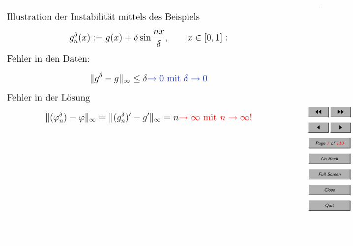
Illustration der Instabilitat mittels des Beispiels

gδn(x) := g(x) + δ sin

nx

δ, x ∈ [0, 1] :

Fehler in den Daten:

‖gδ − g‖∞ ≤ δ→ 0 mit δ → 0

Fehler in der Losung

‖(ϕδn)− ϕ‖∞ = ‖(gδ

n)′ − g′‖∞ = n→∞ mit n→∞!

JJ II

J I

of 110

Go Back

Full Screen

Close

Quit

Losung des inversen Problems mittels Differenzenquotienten:

(Rhg)(x) :=g(x+ h)− g(x− h)

2h, x ∈ [0, 1]

Approximationsfehler:

‖g′ −Rhg‖∞ ≤ h

2‖g′′‖∞, falls g ∈ C2([0, 1])

‖g′ −Rhg‖∞ ≤ h2

6‖g′′′‖∞ falls g ∈ C3([0, 1])

Fortpflanzung des Datenfehlers ‖gδ − g‖∞ ≤ δ:

‖Rhg −Rhgδ‖∞ ≤ δ

hGesamtfehler:

‖g′ −Rhgδ‖∞ ≤ 1

2h‖g′′‖∞ + h−1δ falls g ∈ C2([0, 1]) ,

‖g′ −Rhgδ‖∞ ≤ 1

6h2‖g′′′‖∞︸︷︷︸

→0 fur h→0

+ h−1δ︸︷︷︸→∞ fur h→0

falls g ∈ C3([0, 1]) .

Zwei Terme mit unterschiedlichem Verhalten→ geeignete Wahl von h ist wesentlich!

JJ II

J I

of 110

Go Back

Full Screen

Close

Quit

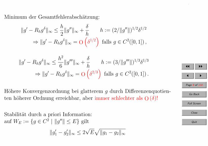
Minimum der Gesamtfehlerabschatzung:

‖g′ −Rhgδ‖∞ ≤ h

2‖g′′‖∞ +

δ

hh := (2/‖g′′‖)1/2δ1/2

⇒ ‖g′ −Rhgδ‖∞ = O

(δ1/2

)falls g ∈ C2([0, 1]) ,

‖g′ −Rhgδ‖∞ ≤ h2

6‖g′′′‖∞ +

δ

hh := (3/‖g′′′‖)1/3δ1/3

⇒ ‖g′ −Rhgδ‖∞ = O

(δ2/3

)falls g ∈ C2([0, 1]) .

Hohere Konvergenzordnung bei glatterem g durch Differenzenquotien-ten hoherer Ordnung erreichbar, aber immer schlechter als O (δ)!

Stabilitat durch a priori Information:auf WE := g ∈ C2 | ‖g′′‖ ≤ E gilt

‖g′1 − g′2‖∞ ≤ 2√E

√‖g1 − g2‖∞

JJ II

J I

of 110

Go Back

Full Screen

Close

Quit

Typische Eigenschaften inverser Probleme anhand dieses Beispiels:

• Formulierung als Intergralgleichung erster Art moglich (muss abernicht sein)

• Verstarkung hochfrequenter Datenfehler

• Instabilitat aufgrund der durch die naturlichen Gegebenheiten vorgegebeneWahl der Normen

• Zuruckgewinnen von Stabilitat durch a-priori Information

• Kompromiss zwischen Genauigkeit und Stabilitat bei der Wahl desDiskretisierungsparameters h

• Abhangigkeit der optimalen Wahl von h und der Konvergenzratevon der Glattheit der Losung

• Ideale Konvergenzrate O (δ) nicht erreichbar

JJ II

J I

of 110

Go Back

Full Screen

Close

Quit

Example 2. (Ruckwarts Warmeleitungsgleichung)Rand-Anfangswertproblem fur die Warmeleitungsgleichung WLG

∂

∂tu(x, t) = ∆u(x, t), x ∈ (0, 1), t ∈ (0, T ),

u(0, t) = u(1, t) = 0, t ∈ (0, T ],

u(x, 0) = ϕ(x), x ∈ [0, 1].

Direktes Problem: Gegeben die Anfangstemperatur ϕ ∈ L2([0, 1]),bestimme die Endtemperatur g = u(·, T ), wobei u : [0, 1] ×[0, T ] → R die WLG mit RB lost.

Inverses Problem: Gegeben die Endtemperatur g = u(·, T ) ∈L2([0, 1]), bestimme die Anfangstemperatur ϕ ∈ L2([0, 1]),wobei u : [0, 1]× [0, T ] → R die WLG mit RB lost.

Losungsansatz mittels Fourierreihenentwicklung:VONS

√2 sin(πn·) : n = 1, 2, . . . von L2([0, 1]),

ϕ(x) =√

2∞∑

n=1

ϕn sin(πnx)

JJ II

J I

of 110

Go Back

Full Screen

Close

Quit

mit ϕn :=√

2∫ 1

0 sin(πnx)ϕ(x) dx,

u(x, t) =√

2∞∑

n=1

un(t) sin(πnx)

Einsetzen in die WLG liefert

u(x, t) =√

2∞∑

n=1

ϕne−π2n2t sin(nπx)

Wie man leicht zeigen kann (Ubung!) ist u ∈ C∞([0, 1] × (0, T ]), lostdie WLG mit RB und erfullt die AB im L2-Sinn u(·, t) → ϕ fur t → 0in L2([0, 1]).Mit dem direkten Losungsoperator (“Vorwartsoperator”) TBH : L2([0, 1]) →L2([0, 1]) definiert durch

(TBHϕ)(x) := 2

∫ 1

0

∞∑n=1

(e−π2n2T sin(nπx) sin(nπy)

)ϕ(y) dy,

Formulierung des Inversen Problems als Integralgleichung erster Art

TBHϕ = g.

JJ II

J I

of 110

Go Back

Full Screen

Close

Quit

Vorwartsoperator wirkt stark glattend (Glattungseigenschaft der WLG!):Dampfung hoher Frequenzen mit Faktor e−π2n2T

→ Nicht-Existenz einer Losung falls die Daten nicht C∞ sind→ Datenfehler in der nten Fourierkomponente von g wird mit Faktoreπ2n2T verstarkt!

⇒ Extrem instabiles inverses Problem!

JJ II

J I

of 110

Go Back

Full Screen

Close

Quit

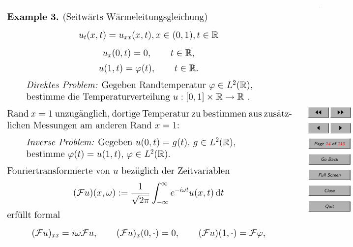
Example 3. (Seitwarts Warmeleitungsgleichung)

ut(x, t) = uxx(x, t), x ∈ (0, 1), t ∈ R

ux(0, t) = 0, t ∈ R,u(1, t) = ϕ(t), t ∈ R.

Direktes Problem: Gegeben Randtemperatur ϕ ∈ L2(R),bestimme die Temperaturverteilung u : [0, 1]× R → R .

Rand x = 1 unzuganglich, dortige Temperatur zu bestimmen aus zusatz-lichen Messungen am anderen Rand x = 1:

Inverse Problem: Gegeben u(0, t) = g(t), g ∈ L2(R),bestimme ϕ(t) = u(1, t), ϕ ∈ L2(R).

Fouriertransformierte von u bezuglich der Zeitvariablen

(Fu)(x, ω) :=1√2π

∫ ∞

−∞e−iωtu(x, t) dt

erfullt formal

(Fu)xx = iωFu, (Fu)x(0, ·) = 0, (Fu)(1, ·) = Fϕ,

JJ II

J I

of 110

Go Back

Full Screen

Close

Quit

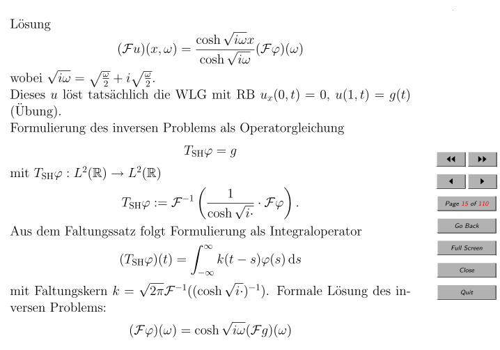
Losung

(Fu)(x, ω) =cosh

√iωx

cosh√iω

(Fϕ)(ω)

wobei√iω =

√ω2 + i

√ω2 .

Dieses u lost tatsachlich die WLG mit RB ux(0, t) = 0, u(1, t) = g(t)(Ubung).Formulierung des inversen Problems als Operatorgleichung

TSHϕ = g

mit TSHϕ : L2(R) → L2(R)

TSHϕ := F−1(

1

cosh√i·· Fϕ

).

Aus dem Faltungssatz folgt Formulierung als Integraloperator

(TSHϕ)(t) =

∫ ∞

−∞k(t− s)ϕ(s) ds

mit Faltungskern k =√

2πF−1((cosh√i·)−1). Formale Losung des in-

versen Problems:

(Fϕ)(ω) = cosh√iω(Fg)(ω)

JJ II

J I

of 110

Go Back

Full Screen

Close

Quit

Die invers Fouriertransformierte der rechten Seite existiert aber nur furDaten g, fur die (Fg)(ω) mit ω → ∞ schneller als 1

cosh√

iωfallt, d.h.,

nur fur sehr glatte Daten!Datenfehler der Frequenz ω wird mit Faktor cosh

√iω verstarkt!

⇒ Extrem instabiles inverses Problem!

JJ II

J I

of 110

Go Back

Full Screen

Close

Quit

Example 4. (Deblurring of images; Hubble space telescope)true image ϕ, blurred image g; integral equation of the first kind∫ ∞

−∞

∫ ∞

−∞k(x, y;x′, y′)ϕ(x′, y′) dx′ dy′ = g(x, y)

k. . . blurring function.usual assumption: k(x, y;x′, y′) spatially invariant, i.e., depends onlyon the distance between the two pixels (x, y), (x′, y′)

k(x, y;x′, y′) = h(x− x′, y − y′), x, x′, y, y′ ∈ R.

h . . . point spread function.convolution integral operator

(TDBϕ)(x, y) :=

∫ ∞

−∞

∫ ∞

−∞h(x− x′, y − y′)ϕ(x′, y′) dx′ dy′.

direct problem: given ϕ, evaluate TDBϕ

inverse problem: given g solve

TDBϕ = g

JJ II

J I

of 110

Go Back

Full Screen

Close

Quit

in principle solvable by Fourier transformation (analogously to sidewaysheat equation)

ϕ = (2π)−1F−1(Fg/Fh)instability due to Fh(ω) → 0 as ω →∞.

JJ II

J I

of 110

Go Back

Full Screen

Close

Quit

Example 5. (Computerized tomography)application: medical imaging and nondestructive testing.X-ray tomography: Determine density ϕ of a two dimensional cross sec-tion of a body from measurements of the attenuation of X-rays goingthrough the body.I(t) = Iϑ,s(t). . . Intensity of an X-ray travelling in direction ϑ⊥ alongthe line t 7→ sϑ + tϑ⊥ where ϑ ∈ S1 := x ∈ R2 : ‖x‖ = 1 and

ϑ⊥ :=

(0 1−1 0

)ϑ.

relative decrease of intensity proportional to density and travelling dis-tance:

−dII

= ϕ dt

with dt→ 0: differential equation

I ′(t) = −ϕ(sϑ+ tϑ⊥)I(t)

explicit solution

I(t) = I(−∞) exp

(−

∫ t

−∞ϕ(sϑ+ tϑ⊥) dt

).

JJ II

J I

of 110

Go Back

Full Screen

Close

Quit

I(±∞)= measured intensity at emitter/detector.ϕ assumed to have compact support K (density in air =0).

− lnIϑ,s(∞)

Iϑ,s(−∞)= (Rϕ)(ϑ, s)

R. . .Radon transform

(Rϕ)(ϑ, s) :=

∫ ∞

−∞ϕ(sϑ+ tϑ⊥) dt.

direct problem: given density distribution ϕ, evaluate Radontransform (Rϕ)(ϑ, s), in all points given by ϑ ∈ S1 and s ∈ R.

inverse problem: determine ϕ ∈ L2(R2), supp(ϕ) ⊆ K frommeasurements of g = Rϕ ∈ L2(S1 × R).

JJ II

J I

of 110

Go Back

Full Screen

Close

Quit

special case: K = B2 := x ∈ R2 : ‖x‖ ≤ 1 and ϕ radially symmetr.:(Rϕ)(ϑ, s) constant in ϑ.⇒ X-rays from one direction uniquely determine ϕ.Set ϕ(x) = Φ(‖x‖2),

(Rϕ)(ϑ, s) =

∫ √1−s2

−√

1−s2

ϕ(sϑ+ tϑ⊥) dt = 2

∫ √1−s2

0Φ(t2 + s2) dt

(Substitution τ := t2 + s2 , σ := s2)

=

∫ 1

σ

Φ(τ)√τ − σ

dτ

→ Abel’s integral equation

(TCTΦ)(σ) = g(σ), σ ∈ [0, 1]

with the Volterra integral operator

(TCTΦ)(σ) :=

∫ 1

σ

Φ(τ)√τ − σ

dτ.

Abel’s integral equation “half as unstable” as differentiation.extreme instability in general case due to lack of full data (limited angleproblems).

JJ II

J I

of 110

Go Back

Full Screen

Close

Quit

Example 6. (Electrical impedance tomography, EIT)D ⊂ Rd, d = 2, 3 electrically conditive material with spatially varyingconductivity σ(x). Due to a voltage impressed at electrodes attachedto the surface, an electric field ~E is generated which is irrotational andtherewith has a potential u such that E = − gradu.We consider the steady state case ∂tE = 0.Ohm’s law: electric current density j

j = σE = −σ gradu .

Gauss’ law (j source free):

div σ gradu = 0, in D.

voltage at the boundary prescribed

u = uimp auf ∂D

electric potential unique only up to a constant: normalization∫∂D

u ds = 0.

JJ II

J I

of 110

Go Back

Full Screen

Close

Quit

measured surface charge

σ∂u

∂ν= q, on ∂D ,

from Gauss’ law (conservation of charges) it follows that∫∂D

q ds = 0.

direct problem: given σ, determine all possible voltage-chargecombinations according to the PDE by solving the ellipticboundary value problem. (Neumann-to-Dirichlet map Λσ :H−1/2(∂D) → H1/2(∂D) defined by Λσq = u|∂D.)

inverse problem: given measurements of the charge distribu-tion for all possible voltages, u|∂D, i.e., given the Neumann-to-Dirichlet map Λσ, reconstruct σ.

Identifiability: Is σ uniquely determined by Λσ?Nonlinear inverse problem, although PDE is linear.Parameter identification problem.

JJ II

J I

of 110

Go Back

Full Screen

Close

Quit

Example 7. (Groundwater modelling)simplified model of goundwater flow: parabolic PDE

S∂u

∂t− div(a gradu) = f in Ω× (0, T ) ,

in a two-dimensional domain Ω ⊆ R2.a. . . transmissivity, S . . . storage coefficient,u. . . piezometric head, f . . . sinks and sources.Steady state case ∂f

∂t = 0, ∂u∂t = 0 → elliptic PDE

− div(a gradu) = f in Ω .

direct problem: given a, f and boundary values of u,determine u by solving the elliptic boundary value problem.

inverse problem: given f and measurements of u in Ω, deter-mine the transmissivity distribution a.

difference to EIT: interior instead of boundary measurements.

JJ II

J I

of 110

Go Back

Full Screen

Close

Quit

1-d case with known a(0)u′(0): explicit solution of the inverse problem:

a(x) =−

∫ x

0 f(ξ) dξ + a(0)u′(0)

u′(x)

provided u′(x) vanishes nowhere.Instability by differentiation of the data; addititional instability by pos-sible smallness of u′(x) and in the 2-d case, by anisotropy: a solves thehyperbolic PDE

div(a gradu) + a∆u = −f

JJ II

J I

of 110

Go Back

Full Screen

Close

Quit

Example 8. (Inverse scattering problems)Important class of inverse problems, applications in acoustics, electro-magnetics, elasticity, quantum theory.Aim: Identification of properties of inacessible objects by measuringwaves scattered by them.Acoustic case: wave equation for velocity potential U

1

c2∂2

∂t2U −∆U = 0

time harmonic case, frequency ω, U(x, t) = Re(u(x)e−iωt),space dependent part u solves Helmholtz equation

∆u+ k2u = 0 in Rd\K.k = ω/c . . . wave number, K . . . impenetrable bounded smooth obstacle.Boundary conditions on ∂K depend on surface properties, e.g. soundsoft obstacle Dirichlet conditions

u = 0 on ∂K.

total field u is superposition u = ui + us

ui . . . known incident field ui(x) = eik〈x,d〉, d ∈ x ∈ R2 : ‖x‖ = 1:us. . . unknown scattered field

JJ II

J I

of 110

Go Back

Full Screen

Close

Quit

Sommerfeld’s radiation condition

limr→∞

r(d−1)/2(∂us

∂r− ikus

)= 0 r = ‖x‖, uniformly for all x = x/r,

(asymptotically energy is transported away from the origin)⇒ scattered field asymptotically behaves like an outgoing wave:

us(x) =eikr

r(d−1)/2

(u∞(x) + O

(1

‖x‖

)), ‖x‖ → ∞

u∞. . . far field pattern or scattering amplitude of us

u∞ : Sd−1 → C definined on Sd−1 := x ∈ Rd : ‖x‖ = 1.

direct problem: given a bounded smooth obstacleK and an in-coming wave ui, determine the far field pattern u∞ ∈ L2(Sd−1)of the scattered field.

inverse problem: given the far field pattern u∞ ∈ L2(Sd−1)and the incident wave ui, determine the obstacle K (e.g., aparametrization of its boundary ∂K).

JJ II

J I

of 110

Go Back

Full Screen

Close

Quit

usually the far field operator F : K 7→ u∞ is infinitely smoothing andtherewith the inverse problem extremely ill-posed.Inverse scattering problems are nonlinear.

JJ II

J I

of 110

Go Back

Full Screen

Close

Quit

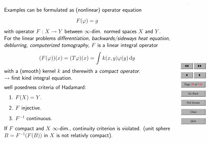
Examples can be formulated as (nonlinear) operator equation

F (ϕ) = g

with operator F : X → Y between ∞-dim. normed spaces X and Y .For the linear problems differentiation, backwards/sideways heat equation,deblurring, computerized tomography, F is a linear integral operator

(F (ϕ))(x) = (Tϕ)(x) =

∫k(x, y)ϕ(y) dy

with a (smooth) kernel k and therewith a compact operator.→ first kind integral equation.

well posedness criteria of Hadamard:

1. F (X) = Y .

2. F injective.

3. F−1 continuous.

If F compact and X ∞-dim., continuity criterion is violated. (unit sphereB = F−1(F (B)) in X is not relativly compact).

JJ II

J I

of 110

Go Back

Full Screen

Close

Quit

We will only consider inverse problems in the sense of identification (deter-mining caused for observed effects).Inverse problems in the sense of determining causes for desired effects willbe treated in the optimization lecture.

Analogies to optimization:formulation of F (ϕ) = g as optimization problem

‖F (ϕ)− g‖ = min! ϕ ∈ X.

Differences to optimization:

Identification: convergence in preimage space,Instability,Identifiability importantExistence natural for exact data

Optimization: convergence in image space (decrease of objective value),Non-uniqueness not problematic,

JJ II

J I

of 110

Go Back

Full Screen

Close

Quit

2. Algoritms for the solution of linear ill-posed prob-lems

Linear ill-posed operator equation

Tϕ = g,

with T : X → Y linear bounded injective operator between Hilbert spacesX and Y and g ∈ R(T ).noisy data gδ given with noise level δ

‖gδ − g‖ ≤ δ.

T not boundedly invertible⇒ Regularization necessary.

JJ II

J I

of 110

Go Back

Full Screen

Close

Quit

2.1. Tikhonov regularization

Equivalent formulation

‖Tϕ− gδ‖2 = minφ∈X

!

regularization by adding a regularization term that penalzes large distancefrom ϕ0:

Jα(ϕ) := ‖Tϕ− gδ‖2 + α‖ϕ− ϕ0‖2 = minφ∈X

!

Jα. . . Tikhonov functionalα > 0. . . regularization parameterif no initial guess available: ϕ0 := 0.

Theorem 1. For any α > 0, gδ ∈ Y and ϕ0 ∈ X there holds:The Tikhonov functional Jα has a unique global minimizer ϕδ

α in X. Itis given by

ϕδα = (T ∗T + αI)−1(T ∗gδ + αϕ0).

The operator T ∗T + αI is boundedly invertible,so ϕδ

α stably depends on gδ.

JJ II

J I

of 110

Go Back

Full Screen

Close

Quit

Definition 2. Let X, Y be normed spaces U an open subset of X. Amapping F : U → Y is called Frechet differentiable in ϕ ∈ U if abounded linear operator T : X → Y exists such that

limh→0

1

‖h‖(F (ϕ+ h)− F (ϕ)− Th) = 0.

T = F ′[ϕ] is called Frechet derivative of F in ϕ. F is called Frechetdifferentiable in U if it is Frechet differentiable in each point ϕ ∈ U .

Lemma 1. Let U be an open subset of a normed space X. If J : U → Ris Frechet differentiable in ϕ and ϕ ∈ U is a local minimizer of J , thenJ ′[ϕ] = 0.

Lemma 2. For all α ≥ 0 the Tikhonov functional is Frechet differen-tiable in X and the Frechet derivative is given by

J ′α[ϕ]h = 2⟨T ∗(Tϕ− gδ) + α(ϕ− ϕ0), h

⟩.

JJ II

J I

of 110

Go Back

Full Screen

Close

Quit

2.2. Landweber Iteration

Minimization of the functional

J0(ϕ) = ‖Tϕ− gδ‖2

by the method of steepest decent; negative gradient:

h = −T ∗(Tϕ− gδ)

ϕ0 = initial guess or 0

ϕn+1 = ϕn − µT ∗(Tϕn − gδ), n ≥ 0,

Landweber iteration.steplength parameter µ such that

µ‖T ∗T‖ ≤ 1.

JJ II

J I

of 110

Go Back

Full Screen

Close

Quit

Expression for nth Landweber iterate

ϕn = (I − µT ∗T )nϕ0 +n−1∑j=0

(I − µT ∗T )jµT ∗gδ.

stopping index n = N plays the role of a regularization parameter: α→ 0for Tikhonov regularization corresponds to n→∞ for Landweber iteration.

µ‖T ∗T‖ ≤ 1 with µ := 1 in principle possible by scaling in Y .

For convergence speed it is important that µ‖T ∗T‖ is close to 1. Estimateof ‖T ∗T‖ analytically or by power method

ψk+1 := T ∗Tψk/‖T ∗Tψk‖.

ψ0 chosen randomly, k ≈ 5 steps.

JJ II

J I

of 110

Go Back

Full Screen

Close

Quit

2.3. Regularization parameter choice: Discrepancy principle

wlog ϕ0 = 0, ϕ ∈ N(T )⊥.decomposition of total error ϕ− ϕδ

α in Tikhonov regularization

ϕ− ϕδα = ϕ− (αI + T ∗T )−1T ∗Tϕ+ (T ∗T + αI)−1T ∗(g − gδ)

= α(αI + T ∗T )−1ϕ︸︷︷︸→0 fur α→0

+ (T ∗T + αI)−1T ∗︸︷︷︸→∞ fur α→0

(g − gδ)

approximation error α(αI + T ∗T )−1ϕpropagated data noise (T ∗T + αI)−1T ∗(g − gδ).

choice of α: balance between accuracy and stability.

optimal choice of α depends on δ and ϕ (via gδ).well-known parameter choice strategy: Morozov’s discrepancy principle:

on one hand: residual ≈ noise level δ.on the other hand: maximal stability.

α(δ, gδ) := supα > 0 : ‖Tϕδα − gδ‖ ≤ τδ

τ ≥ 1 fixed constant.

JJ II

J I

of 110

Go Back

Full Screen

Close

Quit

Usually it suffices to determine α such that

τ1δ ≤ ‖Tϕδα − gδ‖ ≤ τ2δ

with constants 1 ≤ τ1 < τ2.Computation of α by bisection or Newton’s method forf( 1

α) = ‖Tϕδα − gδ‖2 − (τ1−τ2

2 )2δ2.discrepancy principle for iterative methods (e.g. Landweber)stop iteration as soon as the residual drops below the noise level (times τ)

‖TϕδN − gδ‖ ≤ τδ < ‖Tϕδ

n − gδ‖ ∀n ≤ N − 1.

Existence of α or N according to discrepancy principle: see later.

JJ II

J I

of 110

Go Back

Full Screen

Close

Quit

2.4. Other implicit methods

Repeated application of Tikhonov regularization:Iterated Tikhonov regularization:

ϕδα,0 := ϕ0

ϕδα,n+1 := (T ∗T + αI)−1(T ∗gδ + αϕδ

α,n), n ≥ 0

Operator T ∗T + αI must be inverted (LLT factorized) only once. Repre-sentation of ϕδ

α,n (wlog ϕ0 = 0)

ϕδα,n := (αI + T ∗T )−n(T ∗T )−1 ((αI + T ∗T )n − αnI)T ∗gδ

n fixed, α as regularization parameter: iterated Tikhonov regularization.α fixed, n as regularization parameter: iterative method: Lardy’s method.

JJ II

J I

of 110

Go Back

Full Screen

Close

Quit

Other regularization terms:

differential operator L

‖Tϕ− gδ‖2 + α‖L(ϕ− ϕ0)‖2 = min!

damping of nonsmooth parts in the solution.If N(L) = 0: analogously to original Tikhonov regularization withXL := D(L) ⊂ X and the norm ‖ϕ‖XL

:= ‖Lϕ‖X .(spectral theory: XL complete if L selfadjoint and ‖Lϕ‖ ≥ γ‖ϕ‖ for aγ > 0 and all ϕ ∈ D(L).)

If 0 < dimN(L) < ∞ and ‖Tϕ‖2 + ‖Lϕ‖2 ≥ γ‖ϕ‖2 for a γ > 0 andall ϕ ∈ D(L) convergence can still be shown.

JJ II

J I

of 110

Go Back

Full Screen

Close

Quit

BV Regularization

‖Tϕ− gδ‖2 + α‖ϕ− ϕ0)‖2BV = min!

for smooth ϕ: ‖ϕ‖BV = ‖ϕ‖L1 + ‖ gradϕ‖L1.generally: weak formulation

‖ϕ‖BV := ‖ϕ‖L1 + sup

∫Ωϕ div f dx : f ∈ C1

0(Ω), ‖f‖∞ ≤ 1

(f ∈ C1

0(Ω) ⇔ f ∈ C1(Ω) ∧ supp(f) compact subset of interior of Ω)reconstruction of jumps in the solution (e.g. in image processing).

regularization term nondifferentiable!⇒ difficult analysis and numerics.

Maximum entropy regularization

‖Tϕ− gδ‖2 + α

∫ b

a

ϕ(x) logϕ(x)

ϕ0(x)dx = min!

ϕ0 ≥ 0 (white noise) and ϕ ≥ 0 with∫ϕ dx =

∫ϕ0 dx = 1

(probability density).nonlinear regularization term!

JJ II

J I

of 110

Go Back

Full Screen

Close

Quit

2.5. Other explicit methods

drawback of implicit methods: evaluation and inversion of a matrix repre-senting T (discretization).In many applications it is much easier to evaluate Tv or T ∗w even formany elements v, w than to invert or factorize (T ∗T + αI) (e.g. by FFTfor convolution integral operators or fast solvers for PDEs in parameteridentification).→ explicit methods (e.g. Landweber)

Krylov subspace methods, CG:

nth Landweber iterate (with ϕ0 = 0) lies in the nth Krylov subspace

Kn(T∗T, T ∗gδ) := span(T ∗T )jT ∗gδ : j = 1, . . . , n

Improvement of Landweber: define n-the iterate as best approximation inthe nth Krylov subspace.Conjugate gradient method for normal equations

T ∗Tϕ = T ∗y

JJ II

J I

of 110

Go Back

Full Screen

Close

Quit

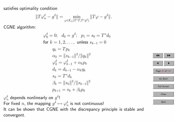
satisfies optimality condition

‖Tϕδn − gδ‖ = min

ϕ∈Kn(T ∗T,T ∗gδ)‖Tϕ− gδ‖.

CGNE algorithm:

ϕδ0 = 0; d0 = gδ; p1 = s0 = T ∗d0

for k = 1, 2, . . . , unless sk−1 = 0

qk = Tpk

αk = ‖sk−1‖2/‖qk‖2

ϕδk = ϕδ

k−1 + αkpk

dk = dk−1 − αkqk

sk = T ∗dk

βk = ‖sk‖2/‖sk−1‖2

pk+1 = sk + βkpk

ϕδn depends nonlinearly on gδ!

For fixed n, the mapping gδ 7→ ϕδn is not continuous!

It can be shown that CGNE with the discrepancy principle is stable andconvergent.

JJ II

J I

of 110

Go Back

Full Screen

Close

Quit

2.6. Quasi solutions

Theorem 2. Let K be a compact topologigal space, and Y a topologicalspace satisfying the Haussdorff separation axiom, let f : K → Y becontinuous and injective.Then f−1 : f(K) → K is continuous with respect to the topology inducedon f(K) by Y .

This immediately implies

Theorem 3. (Tikhonov’s Lemma)Let X, Y be metric spaces, X compakt, f : X → Y continuous andbijective.Then f−1 : Y → X is continuous.

Therewith, the restriction of a continuous injective operator to a compactsubset of the pre-image space is continuously invertible.

JJ II

J I

of 110

Go Back

Full Screen

Close

Quit

Definition 3. Let F : X → Y be a continuous (not necessarily linear)operator and K ⊂ X.ϕδ

K ∈ K is called quasi solution of F (ϕ) = gδ under the constraint K,if

‖F (ϕδK)− gδ‖ = inf

‖F (ϕ)− gδ‖ : ϕ ∈ K

. (∗)

quasi solution exists ⇔ best approximation QF (K)gδ of gδ exists in F (K).

If F (K) closed and convex, QF (K)gδ exists for all gδ ∈ Y , and QF (K) is

continuous.(Note: F linear and K convex ⇒ F (K) convex.)If additionally K ⊂ X compakt:ϕδ

K = (F |K)−1QF (X)gδ continuously depends on gδ.

compact embedding theorems (e.g. Arzela-Ascoli, or Rellich-Kondrachov)→ convex and compact subspaces of X by imposing bounds in strongernorms .e.g. X = L2([0, 1]), K = ϕ ∈ H1

0([0, 1]) : ‖ϕ′‖L2 ≤ R:Tikhonov regularization with differential operator L = d/dx≡ penalty formulation for the constrained optimization problem (*) definingthe quasi solution.

JJ II

J I

of 110

Go Back

Full Screen

Close

Quit

2.7. Regularization by Discretization

Regularization methods for the ∞-dim. operator equation F (ϕ) = g orTϕ = g habe to be discretized for numerical computations.(Discretization error in image space ∼ data noise level)

finite dimensional problems are well-posed in the sense of stability (existenceand uniqueness can be achieved by an appropriate solution concept at leastin the linear case, see the following chapter).

→ Regularization by discretization.

use information on different levels of discretization refinement→ multilevel methods.

JJ II

J I

of 110

Go Back

Full Screen

Close

Quit

3. Regularization Methods

X, Y Hilbert spacesL(X, Y ) space of bounded linear operators X → Y , L(X) := L(X,X)T ∈ L(X, Y ): nullspace N(T ) := ϕ ∈ X : Tϕ = 0, range R(T ) := T (X).

3.1. Orthogonal projections

Theorem 4. Let U be a closed linear subspace of X. Then for anyϕ ∈ X there exists a unique ψ ∈ U such that

‖ψ − ϕ‖ = infu∈U

‖u− ϕ‖.

ψ is called best approximation of ϕ in U .ψ is the unique element in U satisfying

〈ϕ− ψ, u〉 = 0 for all u ∈ U. (∗)The assertion of the theorem remains valid if U is a closed convex subsetof X instead of a linear subspace.Characterization of best approximation ψ (instead of (*))

〈ϕ− ψ, u− ψ〉 ≤ 0 for all u ∈ U.

JJ II

J I

of 110

Go Back

Full Screen

Close

Quit

Definition 4. Let U be a linear subspace of X

U⊥ := v ∈ X : 〈v, u〉 = 0 for all u ∈ U.

Lemma 3. For any linear subspace U of X, U⊥ is a closed linear sub-

space of X and U⊥ = U⊥.

Theorem 5. Let U 6= 0 be a closed linear subspace of X and letP : X → U denote the operator, which maps a vector ϕ ∈ X to itsbest approximation in U . Then P is a linear operator with ‖P‖ = 1satisfying

P 2 = P and P ∗ = P.

P is called orthogonal projection onto U .I − P is the orthogonal projection onto U⊥. Moreover,

X = U ⊕ U⊥ and U⊥⊥ = U.

Theorem 6. If T ∈ L(X, Y ) then

N(T ) = R(T ∗)⊥ and R(T ) = N(T ∗)⊥.

JJ II

J I

of 110

Go Back

Full Screen

Close

Quit

3.2. The Moore-Penrose generalized inverse

Tϕ = g

T ∈ L(X, Y ), T not necessarily injective, g may not lie in R(T ).→ generalized solution concept → generalized notion of inverse

Definition 5. ϕ is called a least-squares solution of Tφ = g if

‖Tϕ− g‖ = inf‖Tψ − g‖ : ψ ∈ X.

ϕ ∈ X is called a best approximate solution of Tφ = dg if ϕ is a least-squares solution of Tφ = g and if

‖ϕ‖ = inf‖ψ‖ : ψ is least-squares solution of Tψ = g.

Theorem 7. Let Q : Y → R(T ) denote the orthogonal projection ontoR(T ). Then the following three statements are equivalent:

ϕ is a least-squares solution to Tϕ = g.

Tϕ = Qg

T ∗Tϕ = T ∗g

JJ II

J I

of 110

Go Back

Full Screen

Close

Quit

Equation T ∗Tϕ = T ∗g is called the normal equation of Tϕ = g.

A least-squares solution of Tφ = g exists if and only if g ∈ R(T )+R(T )⊥.

P : X → N(T ) . . . orthogonal projection onto N(T ) of T ,ϕ0 a least-squares solution to Tϕ = y (if it exists!)⇒ set of all least-squares solutions = ϕ0 + u : u ∈ N(T ),⇒ best approximate solution (I − P )ϕ0.A best-approximate solution of Tϕ = g is unique if it exists.

Definition 6. The Moore-Penrose (generalized) inverseT † : D(T †) → X of T defined on D(T †) := R(T ) + R(T )⊥ maps g ∈D(T †) to the best-approximate solution of Tϕ = g.

T † = T−1 if R(T )⊥ = 0 and N(T ) = 0.

T †g is not defined for all g ∈ Y if R(T ) is not closed!

with T : N(T )⊥ → R(T ), Tϕ := Tϕ . . . restriction of T to N(T )⊥:

T †g = T−1Qg for all g ∈ D(T †).

JJ II

J I

of 110

Go Back

Full Screen

Close

Quit

The Moore-Penrose inverse T † is equivalently characterized by the Moore-Penrose equations:

TT †T = T

T †TT † = T †

T †T = I − P

TT † = Q

where P,Q are the orthogonal projections onto N(T ) and R(T ), respec-tively.

JJ II

J I

of 110

Go Back

Full Screen

Close

Quit

3.3. Definition and properties of regularization methods

Definition 7. .(Rα : Y → X)α∈A . . . family of continuous (nonlinear) operators

α : (0,∞)× Y → A, (δ, gδ) 7→ α(δ, gδ) . . . parameter choice rule.

T †g ≈ Rα(δ,gδ)gδ.

The pair (R,α) is called a regularization method for Tϕ = g if

limδ→0

sup∥∥Rα(δ,gδ)g

δ − T †g∥∥ : gδ ∈ Y, ‖gδ − g‖ ≤ δ

= 0 for all g ∈ D(T †)

α is called a-priori parameter choice rule if α(δ, gδ) depends only on δ.Otherwise α is called a-posteriori parameter choice rule.

Tikhonov regularization: A = (0,∞) and Rα = (αI + T ∗T )−1T ∗.

Landweber iteration: A = 1n : n ∈ N, andRα =

∑1/αj=0(I−µT ∗T )jµT ∗gδ.

Discrepancy principle . . . a-posteriori parameter choice rule.

α(δ, gδ) = δ . . . a priori parameter choice rule for Tikhonov.


δ − T †g∥∥ : gδ ∈ Y, ‖gδ − g‖ ≤ δ

. . . worst case error

JJ II

J I

of 110

Go Back

Full Screen

Close

Quit

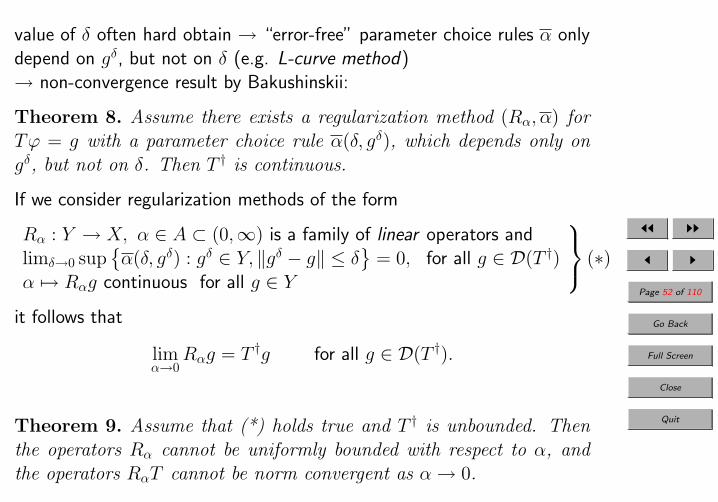
value of δ often hard obtain → “error-free” parameter choice rules α onlydepend on gδ, but not on δ (e.g. L-curve method)→ non-convergence result by Bakushinskii:

Theorem 8. Assume there exists a regularization method (Rα, α) forTϕ = g with a parameter choice rule α(δ, gδ), which depends only ongδ, but not on δ. Then T † is continuous.

If we consider regularization methods of the form

Rα : Y → X, α ∈ A ⊂ (0,∞) is a family of linear operators andlimδ→0 sup

α(δ, gδ) : gδ ∈ Y, ‖gδ − g‖ ≤ δ

= 0, for all g ∈ D(T †)

α 7→ Rαg continuous for all g ∈ Y

(∗)

it follows that

limα→0

Rαg = T †g for all g ∈ D(T †).

Theorem 9. Assume that (*) holds true and T † is unbounded. Thenthe operators Rα cannot be uniformly bounded with respect to α, andthe operators RαT cannot be norm convergent as α→ 0.

JJ II

J I

of 110

Go Back

Full Screen

Close

Quit

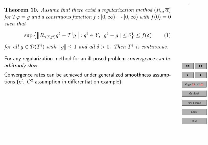
Theorem 10. Assume that there exist a regularization method (Rα, α)for Tϕ = g and a continuous function f : [0,∞) → [0,∞) with f(0) = 0such that


δ − T †g∥∥ : gδ ∈ Y, ‖gδ − g‖ ≤ δ

≤ f(δ) (1)

for all g ∈ D(T †) with ‖g‖ ≤ 1 and all δ > 0. Then T † is continuous.

For any regularization method for an ill-posed problem convergence can bearbitrarily slow.

Convergence rates can be achieved under generalized smoothness assump-tions (cf. C2-assumption in differentiation example).

JJ II

J I

of 110

Go Back

Full Screen

Close

Quit

4. Spectral theory

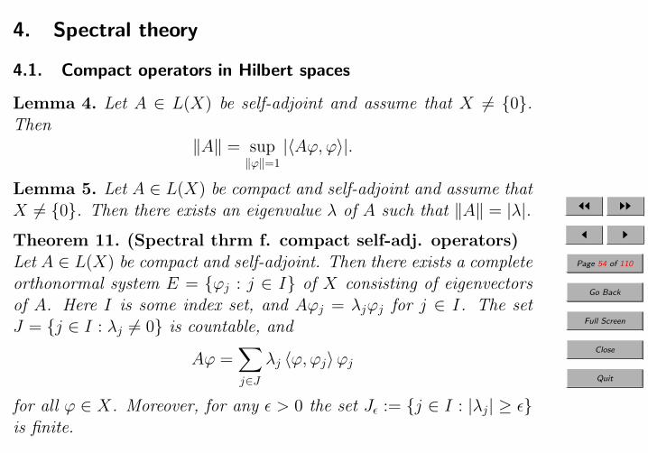
4.1. Compact operators in Hilbert spaces

Lemma 4. Let A ∈ L(X) be self-adjoint and assume that X 6= 0.Then

‖A‖ = sup‖ϕ‖=1

|〈Aϕ,ϕ〉|.

Lemma 5. Let A ∈ L(X) be compact and self-adjoint and assume thatX 6= 0. Then there exists an eigenvalue λ of A such that ‖A‖ = |λ|.

Theorem 11. (Spectral thrm f. compact self-adj. operators)Let A ∈ L(X) be compact and self-adjoint. Then there exists a completeorthonormal system E = ϕj : j ∈ I of X consisting of eigenvectorsof A. Here I is some index set, and Aϕj = λjϕj for j ∈ I. The setJ = j ∈ I : λj 6= 0 is countable, and

Aϕ =∑j∈J

λj 〈ϕ, ϕj〉ϕj

for all ϕ ∈ X. Moreover, for any ε > 0 the set Jε := j ∈ I : |λj| ≥ εis finite.

JJ II

J I

of 110

Go Back

Full Screen

Close

Quit

Theorem 12. and Definition (Singular value decomposition)Let T ∈ L(X, Y ) be compact, and let P ∈ L(X) denote the orthogonalprojection onto N(T ). Then there exist singular values σ0 ≥ σ1 ≥ . . . >0 and orthonormal systems ϕ0, ϕ1, . . . ⊂ X and g0, g1, . . . ⊂ Y suchthat for all

ϕ =∞∑

n=0

〈ϕ, ϕn〉ϕn + Pϕ and Tϕ =∞∑

n=0

σn 〈ϕ, ϕn〉 gn.

A system (σn, ϕn, gn) with these properties is called a singular systemof T . It is uniquely characterized by

Tϕn = σngn and T ∗gn = σnϕn ∀n ∈ N

If dimR(T ) < ∞, the series degenerate to finite sums. The singularvalues σn = σn(T ) are uniquely determined by T and satisfy

σn(T ) → 0 as n→∞.

If dimR(T ) <∞ and n ≥ dimR(T ), we set σn(T ) := 0.

JJ II

J I

of 110

Go Back

Full Screen

Close

Quit

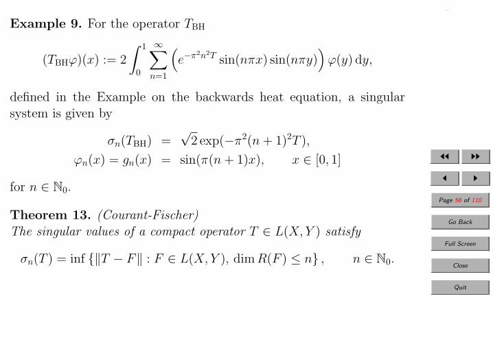
Example 9. For the operator TBH

(TBHϕ)(x) := 2

∫ 1

0

∞∑n=1

(e−π2n2T sin(nπx) sin(nπy)

)ϕ(y) dy,

defined in the Example on the backwards heat equation, a singularsystem is given by

σn(TBH) =√

2 exp(−π2(n+ 1)2T ),

ϕn(x) = gn(x) = sin(π(n+ 1)x), x ∈ [0, 1]

for n ∈ N0.

Theorem 13. (Courant-Fischer)The singular values of a compact operator T ∈ L(X, Y ) satisfy

σn(T ) = inf ‖T − F‖ : F ∈ L(X, Y ), dimR(F ) ≤ n , n ∈ N0.

JJ II

J I

of 110

Go Back

Full Screen

Close

Quit

Theorem 14. (Picard) Let T ∈ L(X, Y ) be compact, and let (σn, ϕn, gn)be a singular system of T . Then the equation Tϕ = g is solvable if andonly if g ∈ N(T ∗)⊥ and if the Picard criterion

∞∑n=0

1

σ2n

| 〈g, gn〉 |2 <∞

is satisfied. Then the solution is given by

ϕ =∞∑

n=0

1

σn〈g, gn〉ϕn.

Picard criterion illustrates ill-posedness of linear operator equations witha compact operator: since 1/σn → ∞ large Fourier modes are amplifiedwithout bound. Typically, large Fourier modes correspond to high frequen-cies. The faster the σn decay of, the more severe is the ill-posedness.

Tϕ = g. . . mildly ill-posed ⇔ ∃C, p > 0 : σn ≥ Cn−p for all n ∈ N.Otherwise Tϕ = g. . . severely ill-posed.Tϕ = g. . . exponentially ill-posed ⇔ ∃C, p > 0 :σn ≤ C exp(−np).

JJ II

J I

of 110

Go Back

Full Screen

Close

Quit

Restore stability by truncating the series:

Rαg :=∑

n:σn≥α

1

σn〈g, gn〉ϕn.

for some α > 0: truncated singular value decomposition. Modified version

Rαg :=∑

n:σn≥α

1

σn〈g, gn〉ϕn.+

∑n:σn<α

1

α〈g, gn〉ϕn.

Numerical computation of singular system too costly.For certain problems analytical expressions for singular system known.

Truncated SVD can be seen as special case of regularization by discretiza-tion:

Projspangj : j∈Iα(TProjspanϕj : j∈Iαϕ− gδ) = 0

with Iα = n ∈ N0 : σn ≥ α.

JJ II

J I

of 110

Go Back

Full Screen

Close

Quit

4.2. The spectral theorem for bounded self-adjoint operators

Generalization of SVD to bounded (not necessarily compact) operators.

Reformulate spectral theorem for compact self-adjoint operators:Hilbert space l2(I) of functions f : I → C with norm ‖f‖2 :=

∑j∈J |f(j)|2.

Define operator W : l2(I) → X by W (f) :=∑

j∈I f(j)ϕj.Parseval’s equality ⇒ W unitary.(W−1ϕ)(j) = 〈ϕ, ϕj〉 for j ∈ I.

Aϕ =∑j∈I

λj 〈ϕ, ϕj〉ϕj

is equivalent to

A = WMλW−1 ⇔ W−1AW = Mλ

where Mλ ∈ L(l2(I)) is defined by (Mλf)(j) = λjf(j), j ∈ I.There exists a unitary map W such that A is transformed to themultiplication operator Mλ on l2(I).

JJ II

J I

of 110

Go Back

Full Screen

Close

Quit

Class of examples of inverse problems with noncompact forward operators:convolution integral equations.k : Rd → C, k ∈ L1(Rd), k(−x) = k(x) for x ∈ Rd.

(Aϕ)(x) :=

∫Rd

k(x− y)ϕ(y) dy

A is self-adjoint, A ∈ L(X) with X = L2(Rd).Fourier transform

(Fϕ)(ω) := (2π)−d/2∫

Rd

e−i〈ω,x〉ϕ(x) dx, ω ∈ Rd

is unitary on L2(Rd) (Plancherel) and inverse operator is given by

(F−1f)(x) := (2π)−d/2∫

Rd

ei〈ω,x〉f(ω) dω, x ∈ Rd.

k(−x) = k(x) ⇒ Fk real-valuedk ∈ L1(Rd) ⇒ Fk ∈ L∞(Rd).

with λ := (2π)d/2Fk,Mλ ∈ L(L2(Rd)), defined by (Mλf)(ω) := λ(ω)f(ω)we get

FAF−1 = Mλ.

JJ II

J I

of 110

Go Back

Full Screen

Close

Quit

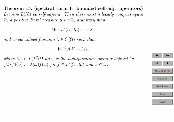
Theorem 15. (spectral thrm f. bounded self-adj. operators)Let A ∈ L(X) be self-adjoint. Then there exist a locally compact spaceΩ, a positive Borel measure µ on Ω, a unitary map

W : L2(Ω, dµ) −→ X,

and a real-valued function λ ∈ C(Ω) such that

W−1AW = Mλ,

where Mλ ∈ L(L2(Ω, dµ)) is the multiplication operator defined by(Mλf)(ω) := λ(ω)f(ω) for f ∈ L2(Ω, dµ) and ω ∈ Ω.

JJ II

J I

of 110

Go Back

Full Screen

Close

Quit

Lemma 6. Let A ∈ L(X) be self-adjoint. Then the initial value prob-lem

d

dtU(t) = iAU(t), U(0) = I

has a unique solution U ∈ C1(R, L(X)) given by

U(t) =∞∑

n=0

1

n!(itA)n.

U(t) : t ∈ R is a group of unitary operators with

(∗) U(s+ t) = U(s)U(t), U(0) = I

For ϕ ∈ X we call

Xϕ := spanU(t)ϕ : t ∈ R

the cyclic subspace generated by ϕ. We say that ϕ ∈ X is a cyclic vectorof X if Xϕ = X.

Lemma 7. If U(t) is a unitary group on a Hilbert space with (*), thenX is an orthogonal direct sum of cyclic subspaces.

JJ II

J I

of 110

Go Back

Full Screen

Close

Quit

Theorem 16. (Riesz) Let Ω be a locally compact space, and let C0(Ω)denote the space of continuous, compactly supported functions on Ω.Let L : C0(Ω) → R be a positive linear functional, i.e. L(f) ≥ 0 for allf ≥ 0. Then there exists a positive Borel measure µ on Ω such that forall f ∈ C0(Ω)

L(f) =

∫f dµ.

Lemma 8. If U(t) : t ∈ R is a continuous unitary group of operatorson a Hilbert space X, having a cyclic vector ϕ, then there exist a positiveBorel measure µ on R and a unitary map W : L2(R, dµ) → X such that

W−1U(t)Wf(ω) = eitωf(ω), ω ∈ Rfor all f ∈ L2(R, dµ) and t ∈ R.

Lemma 9. Let µ be a Borel measure on a locally compact space Ω,and let a ∈ C(Ω). Then the norm of Ma ∈ L(L2(Ω, dµ)) defined by(Mag)(ω) := a(ω)g(ω) for g ∈ L2(Ω, dµ) and ω ∈ Ω is given by

‖Ma‖ = ‖a‖∞, suppµ

where suppµ = Ω \⋃

S open, µ(S)=0 S.

JJ II

J I

of 110

Go Back

Full Screen

Close

Quit

Definition 8. Let X be a Banach space and A ∈ L(X). The resolventset ρ(A) of A is the set of all λ ∈ C for which N(λI − A) = 0,R(λI − A) = X, and (λI − A) is boundedly invertible. The spectrumof A is defined as σ(A) := C \ ρ(A).

Lemma 10. Let X be a Hilbert space and A ∈ L(X) selfadjoint, let thelocally compact space Ω, the Borel measure µ and λ ∈ C(Ω) be definedaccording to the spectral theorem. Then

σ(A) = λ(suppµ).

σ(A) is closed and bounded and hence compact.

JJ II

J I

of 110

Go Back

Full Screen

Close

Quit

For a polynomial p(λ) =∑n

j=0 pjλj define

p(A) :=n∑

j=0

pjAj. (∗)

Theorem 17. (functional calculus) With the notation of the spectraltheorem for selfadjoint bounded operators define

f(A) := WMfλW−1

for a real-valued function f ∈ C(σ(A)). Here (f λ)(ω) := f(λ(ω)).Then f(A) ∈ L(X) is self-adjoint and satisfies (*) if f is a polynomial.The mapping f 7→ f(A), which is called the functional calculus at A,is an isometric algebra homomorphism from C(σ(A)) to L(X), i.e. forf, g ∈ C(σ(A)) and α, β ∈ R we have

(αf + βg)(A) = αf(A) + βg(A),

(fg)(A) = f(A)g(A), (∗∗)‖f(A)‖ = ‖f‖∞.

The functional calculus is uniquely determined by (*) and (**).

JJ II

J I

of 110

Go Back

Full Screen

Close

Quit

Lemma 11. If T ∈ L(X, Y ) and f ∈ C([0, ‖T ∗T‖]), then

Tf(T ∗T ) = f(TT ∗)T.

M(σ(A)) . . . algebra of bounded, Borel-measureable functions on σ(A)with the norm ‖f‖∞ := supt∈σ(A) |f(t)|.

Theorem 18. For f ∈M(σ(A)), the mapping f 7→ f(A) := WMfλW−1

is a norm-decreasing algebra homomorphism from M(σ(A)) to L(X),i.e. for f, g ∈M(σ(A)) and α, β ∈ R we have

(αf + βg)(A) = αf(A) + βg(A),

(fg)(A) = f(A)g(A),

‖f(A)‖ ≤ ‖f‖∞.

If (fn) is a sequence in M(σ(A)) converging pointwise to a functionf ∈M(σ(A)) such that supn∈N ‖fn‖ <∞, then

‖fn(A)ϕ− f(A)ϕ‖ → 0 as n→∞

for all ϕ ∈ X.

JJ II

J I

of 110

Go Back

Full Screen

Close

Quit

5. Convergence of linear regularization methods

Tϕ = g

T ∈ L(X, Y ) where X, Y are Hilbert spaces.g ∈ D(T †) data gδ ∈ Y satisfy

‖g − gδ‖ ≤ δ.

Regularization methods of the form

Rαgδ := qα(T ∗T )T ∗gδ

with qα ∈ C([0, ‖T ∗T‖])).ϕ† := T †g . . . exact solutionϕα := Rαg. . . reconstructions for exact dataϕδ

α := Rαgδ. . . reconstructions for exact data

Reconstruction error for exact data:

ϕ† − ϕα = (I − qα(T ∗T )T ∗T )ϕ† = rα(T ∗T )ϕ†

withrα(λ) := 1− λqα(λ), λ ∈ [0, ‖T ∗T‖].

JJ II

J I

of 110

Go Back

Full Screen

Close

Quit

Tikhonov qα(λ) =1

λ+ αrα(λ) =

α

λ+ α

iter. Tikh. qα(λ) =(λ+ α)n − αn

λ(λ+ α)nrα(λ) =

(α

λ+ α

)n

trunc. SVD qα(λ) =

1

λ, λ ≥ α

0, λ < αrα(λ) =

0, λ ≥ α1, λ < α

mod. TSVD qα(λ) =

1

λ, λ ≥ α

1

α, λ < α

rα(λ) =

0, λ ≥ α

1− λ

α, λ < α

Landweber

with µ = 1 qn(λ) =∑n−1

j=0 (1− λ)j rn(λ) = (1− λ)n

JJ II

J I

of 110

Go Back

Full Screen

Close

Quit

(∗) limα→0

rα(λ) =

0, λ > 01, λ = 0

=: r0(λ)

(∗∗) |rα(λ)| ≤ Cr for λ ∈ [0, ‖T ∗T‖]

(∗ ∗ ∗) |qα(λ)| ≤ Cq

αfor λ ∈ [0, ‖T ∗T‖]

Condition (*) is equivalent to limα→0 qα(λ) = 1/λ for all λ > 0.

Theorem 19. If (*) and (**) hold true, then the operators Rα definedby Rαy := qα(T ∗T )T ∗y, y ∈ Y converge pointwise to T † on D(T †) asα→ 0. With the additional assumption (***) the norm of the regular-ization operators can be estimated by

‖Rα‖ ≤√

(Cr + 1)Cq

α.

If α(δ, gδ) is a parameter choice rule satisfying

α(δ, gδ) → 0, and δ/√α(δ, gδ) → 0 as δ → 0,

then (Rα, α) is a regularization method.

JJ II

J I

of 110

Go Back

Full Screen

Close

Quit

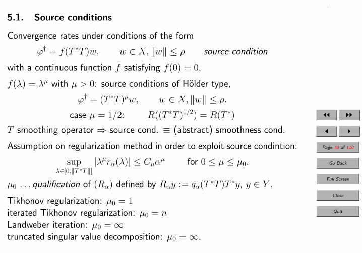
5.1. Source conditions

Convergence rates under conditions of the form

ϕ† = f(T ∗T )w, w ∈ X, ‖w‖ ≤ ρ source condition

with a continuous function f satisfying f(0) = 0.

f(λ) = λµ with µ > 0: source conditions of Holder type,

ϕ† = (T ∗T )µw, w ∈ X, ‖w‖ ≤ ρ.

case µ = 1/2: R((T ∗T )1/2) = R(T ∗)

T smoothing operator ⇒ source cond. ≡ (abstract) smoothness cond.

Assumption on regularization method in order to exploit source condintion:

supλ∈[0,‖T ∗T‖]

|λµrα(λ)| ≤ Cµαµ for 0 ≤ µ ≤ µ0.

µ0 . . . qualification of (Rα) defined by Rαy := qα(T ∗T )T ∗y, y ∈ Y .

Tikhonov regularization: µ0 = 1iterated Tikhonov regularization: µ0 = nLandweber iteration: µ0 = ∞truncated singular value decomposition: µ0 = ∞.

JJ II

J I

of 110

Go Back

Full Screen

Close

Quit

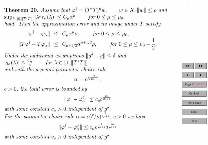
Theorem 20. Assume that ϕ† = (T ∗T )µw, w ∈ X, ‖w‖ ≤ ρ andsupλ∈[0,‖T ∗T‖] |λµrα(λ)| ≤ Cµα

µ for 0 ≤ µ ≤ µ0.hold. Then the approximation error and its image under T satisfy

‖ϕ† − ϕα‖ ≤ Cµαµρ, for 0 ≤ µ ≤ µ0,

‖Tϕ† − Tϕα‖ ≤ Cµ+1/2αµ+1/2ρ, for 0 ≤ µ ≤ µ0 −

1

2.

Under the additional assumptions ‖gδ − g‖ ≤ δ and|qα(λ)| ≤ Cq

α for λ ∈ [0, ‖T ∗T‖]and with the a-priori parameter choice rule

α = cδ2

2µ+1 ,

c > 0, the total error is bounded by

‖ϕ† − ϕδα‖ ≤ cµδ

2µ2µ+1

with some constant cµ > 0 independent of gδ.

For the parameter choice rule α = c(δ/ρ)2

2µ+1 , c > 0 we have

‖ϕ† − ϕδα‖ ≤ cµρ

12µ+1δ

2µ2µ+1

with some constant cµ > 0 independent of gδ.

JJ II

J I

of 110

Go Back

Full Screen

Close

Quit

Holder-type source conditions are far too restrictive for most exponentiallyill-posed problems (implies that ϕ† is an analytic function)

fp(λ) :=

(− lnλ)−p, 0 < λ ≤ exp(−1)0, λ = 0

with p > 0, i.e.ϕ† = fp(T

∗T )w, ‖w‖ ≤ ρ.

logarithmic source condition. avoid the singularity of fp(λ) at λ = 1:assume that ‖T ∗T‖ = ‖T‖2 ≤ exp(−1). (scaling)

JJ II

J I

of 110

Go Back

Full Screen

Close

Quit

Theorem 21. Assume that ϕ† = fp(T∗T )w, ‖w‖ ≤ ρ.

with fp(λ) :=

(− lnλ)−p, 0 < λ ≤ exp(−1)0, λ = 0

, with p > 0 and

supλ∈[0,‖T ∗T‖] |λµrα(λ)| ≤ Cµαµ for 0 ≤ µ ≤ µ0. with µ0 > 0

hold true. Then there exist constants γp > 0 such that the approxima-tion error is bounded by

‖ϕ† − ϕα‖ ≤ γpfp(α)ρ

for all α ∈ [0, exp(−1)]. Under the additional assumptions ‖gδ−g‖ ≤ δand|qα(λ)| ≤ Cq

α for λ ∈ [0, ‖T ∗T‖]and with the a-priori parameter choice rule

α = δ

the total error is bounded by

‖ϕ† − ϕδα‖ ≤ cpfp(δ) for δ ≤ exp(−1)

with some constant cp > 0 independent of gδ. If α = δ/ρ, then

‖ϕ† − ϕδα‖ ≤ cpρfp(δ/ρ), for δ/ρ ≤ exp(−1)

with some constant cp > 0 independent of gδ and ρ.

JJ II

J I

of 110

Go Back

Full Screen

Close

Quit

5.2. Optimality and an abstract stability result

Mf,ρ := ϕ† ∈ X : ϕ† satisfies ϕ† = f(T ∗T )w, ‖w‖ ≤ ρ,

For R : Y → X define worst case error of the method R

∆R(δ,Mf,ρ, T ) := sup‖Rgδ−ϕ†‖ : ϕ† ∈Mf,ρ, gδ ∈ Y, ‖Tϕ†−Qgδ‖ ≤ δ.

Best possible error bound:

∆(δ,Mf,ρ, T ) := infR:Y→X

∆R(δ,Mf,ρ, T )

Theorem 22. Let

ω(δ,Mf,ρ, T ) := sup‖ϕ†‖ : ϕ† ∈Mf,ρ, ‖Tϕ†‖ ≤ δ

denote the modulus of continuity of (T |Mf,ρ)−1. Then

∆(δ,Mf,ρ, T ) ≥ ω(δ,Mf,ρ, T ).

It can be shown that

∆(δ,Mf,ρ, T ) = ω(δ,Mf,ρ, T ).

JJ II

J I

of 110

Go Back

Full Screen

Close

Quit

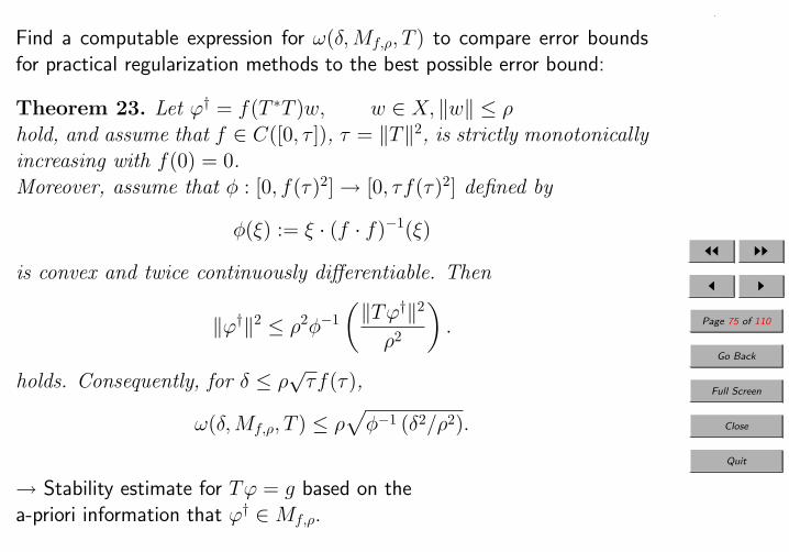
Find a computable expression for ω(δ,Mf,ρ, T ) to compare error boundsfor practical regularization methods to the best possible error bound:

Theorem 23. Let ϕ† = f(T ∗T )w, w ∈ X, ‖w‖ ≤ ρhold, and assume that f ∈ C([0, τ ]), τ = ‖T‖2, is strictly monotonicallyincreasing with f(0) = 0.Moreover, assume that φ : [0, f(τ)2] → [0, τf(τ)2] defined by

φ(ξ) := ξ · (f · f)−1(ξ)

is convex and twice continuously differentiable. Then

‖ϕ†‖2 ≤ ρ2φ−1(‖Tϕ†‖2

ρ2

).

holds. Consequently, for δ ≤ ρ√τf(τ),

ω(δ,Mf,ρ, T ) ≤ ρ√φ−1 (δ2/ρ2).

→ Stability estimate for Tϕ = g based on thea-priori information that ϕ† ∈Mf,ρ.

JJ II

J I

of 110

Go Back

Full Screen

Close

Quit

Lemma 12. (Jensen’s inequality) Assume that φ ∈ C2([α, β]) withα, β ∈ R ∪ ±∞ is convex, and let µ be a finite measure on somemeasure space Ω. Then

φ

(∫χdµ∫dµ

)≤

∫φ χdµ∫dµ

holds for all χ ∈ L1(Ω, dµ) satisfying α ≤ χ ≤ β almost everywhere dµ.The right hand side may be infinite if α = −∞ or β = ∞.

For the special case φ(t) = tp, p > 1, Jensen’s inequality becomes∫χdµ ≤

(∫χpdµ

) 1p(∫

dµ

) 1q

with q = pp−1 , i.e., Holder’s inequality∫

|a||b|dµ ≤(∫

|a|pdµ) 1

p(∫

|b|qdµ) 1

q

for positive measures µ on Ω, a ∈ Lp(µ), and b ∈ Lq(µ)

by setting µ = |b|qµ and χ = |a||b|−1

p−1 .

JJ II

J I

of 110

Go Back

Full Screen

Close

Quit

Definition 9. Let (Rα, α) be a regularization method for Tϕ = g, andlet the assumptions of Theorem 23 be satisfied. Convergence on thesource sets Mf,ρ is said to be

• optimal if∆Rα

(δ,Mf,ρ, T ) ≤ ρ√φ−1 (δ2/ρ2)

• asymptotically optimal if

∆Rα(δ,Mf,ρ, T ) = ρ

√φ−1 (δ2/ρ2) (1 + o (1)), δ → 0

• of optimal order if there is a constant C ≥ 1 such that

∆Rα(δ,Mf,ρ, T ) ≤ Cρ

√φ−1 (δ2/ρ2)

for δ/ρ sufficiently small.

JJ II

J I

of 110

Go Back

Full Screen

Close

Quit

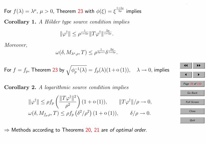
For f(λ) = λµ, µ > 0, Theorem 23 with φ(ξ) = ξ1+2µ2µ implies

Corollary 1. A Holder type source condition implies

‖ϕ†‖ ≤ ρ1

1+2µ‖Tϕ†‖2µ

1+2µ .

Moreover,

ω(δ,Mλµ,ρ, T ) ≤ ρ1

2µ+1δ2µ

1+2µ .

For f = fp, Theorem 23 by√φ−1

p (λ) = fp(λ)(1+o (1)), λ→ 0, implies

Corollary 2. A logarithmic source condition implies

‖ϕ†‖ ≤ ρfp

(‖Tϕ†‖2

ρ2

)(1 + o (1)), ‖Tϕ†‖/ρ→ 0,

ω(δ,Mfp,ρ, T ) ≤ ρfp

(δ2/ρ2) (1 + o (1)), δ/ρ→ 0.

⇒ Methods according to Theorems 20, 21 are of optimal order.

JJ II

J I

of 110

Go Back

Full Screen

Close

Quit

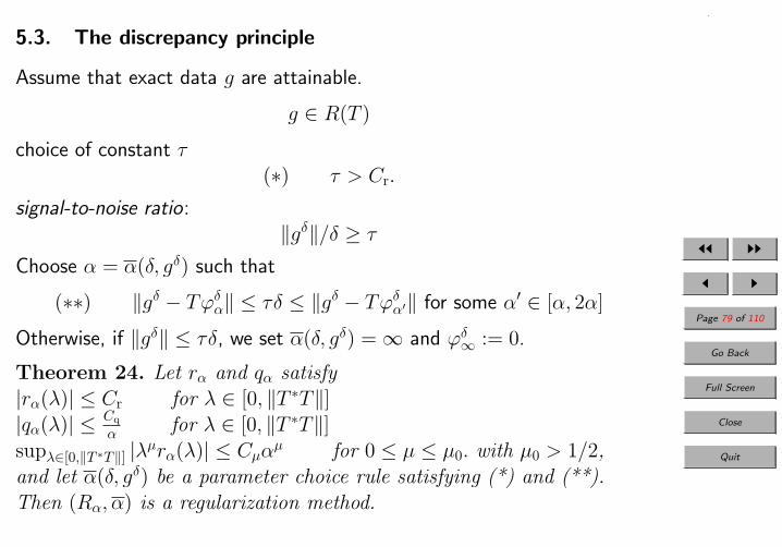
5.3. The discrepancy principle

Assume that exact data g are attainable.

g ∈ R(T )

choice of constant τ(∗) τ > Cr.

signal-to-noise ratio:‖gδ‖/δ ≥ τ

Choose α = α(δ, gδ) such that

(∗∗) ‖gδ − Tϕδα‖ ≤ τδ ≤ ‖gδ − Tϕδ

α′‖ for some α′ ∈ [α, 2α]

Otherwise, if ‖gδ‖ ≤ τδ, we set α(δ, gδ) = ∞ and ϕδ∞ := 0.

Theorem 24. Let rα and qα satisfy|rα(λ)| ≤ Cr for λ ∈ [0, ‖T ∗T‖]|qα(λ)| ≤ Cq

α for λ ∈ [0, ‖T ∗T‖]supλ∈[0,‖T ∗T‖] |λµrα(λ)| ≤ Cµα

µ for 0 ≤ µ ≤ µ0. with µ0 > 1/2,and let α(δ, gδ) be a parameter choice rule satisfying (*) and (**).Then (Rα, α) is a regularization method.

JJ II

J I

of 110

Go Back

Full Screen

Close

Quit

Order optimality :

Holder source conditions:

Theorem 25. Under the assumptions of Theorem 24 let ϕ† satisfy aHolder source condition with 0 < µ ≤ µ0 − 1/2. Then there exists aconstant cµ > 0 independent of ρ, δ, and ϕ† such that

‖ϕ† − ϕα(δ,gδ)‖ ≤ cµρ1

2µ+1δ2µ

2µ+1 .

Logarithmic source conditions: order optimality with discrepancy principle.Modified discrepancy principle: even asymptotically optimal convergence.

JJ II

J I

of 110

Go Back

Full Screen

Close

Quit

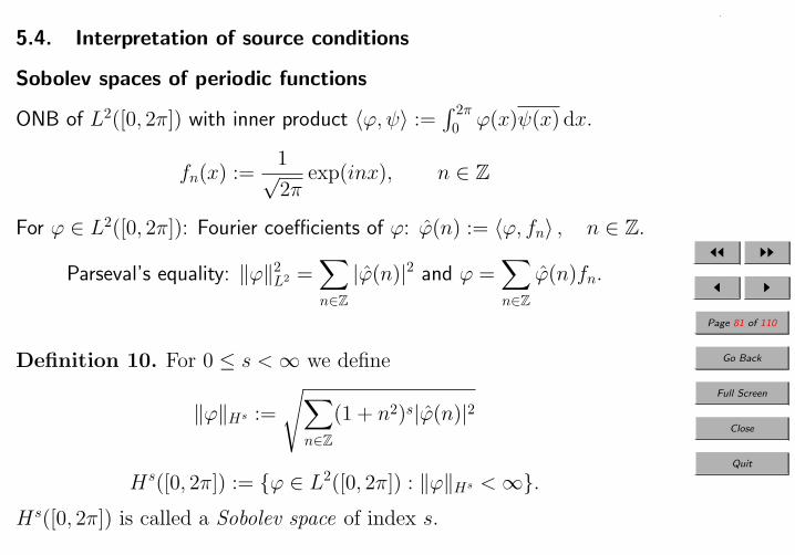
5.4. Interpretation of source conditions

Sobolev spaces of periodic functions

ONB of L2([0, 2π]) with inner product 〈ϕ, ψ〉 :=∫ 2π

0 ϕ(x)ψ(x) dx.

fn(x) :=1√2π

exp(inx), n ∈ Z

For ϕ ∈ L2([0, 2π]): Fourier coefficients of ϕ: ϕ(n) := 〈ϕ, fn〉 , n ∈ Z.

Parseval’s equality: ‖ϕ‖2L2 =

∑n∈Z

|ϕ(n)|2 and ϕ =∑n∈Z

ϕ(n)fn.

Definition 10. For 0 ≤ s <∞ we define

‖ϕ‖Hs :=

√∑n∈Z

(1 + n2)s|ϕ(n)|2

Hs([0, 2π]) := ϕ ∈ L2([0, 2π]) : ‖ϕ‖Hs <∞.Hs([0, 2π]) is called a Sobolev space of index s.

JJ II

J I

of 110

Go Back

Full Screen

Close

Quit

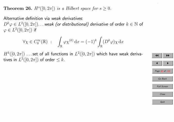
Theorem 26. Hs([0, 2π]) is a Hilbert space for s ≥ 0.

Alternative definition via weak derivatives:Dkϕ ∈ L2([0, 2π]). . . weak (or distributional) derivative of order k ∈ N ofϕ ∈ L2([0, 2π]) if

∀χ ∈ C∞0 (R) :

∫Rϕχ(k) dx = (−1)k

∫R(Dkϕ)χ dx

Hk([0, 2π]) . . . set of all functions in L2([0, 2π]) which have weak deriva-tives in L2([0, 2π]) of order ≤ k.

JJ II

J I

of 110

Go Back

Full Screen

Close

Quit

Holder-type source conditions

Example 10. Numerical differention:Solve TDϕ = g with

(TDϕ)(x) :=

∫ x

0ϕ(t) dt+ c(ϕ), x ∈ [0, 2π]

c(ϕ) := − 12π

∫ 2π

0

∫ x

0 ϕ(t) dt dx

L20([0, 2π]) :=

ϕ ∈ L2([0, 2π]) :

∫ 2π

0ϕ(x) dx = 0

TD ∈ L(L2

0([0, 2π])).

Theorem 27. R((T ∗DTD)µ) = H2µ([0, 2π]) ∩ L20([0, 2π]) for all µ ≥ 0.

Moreover,‖(T ∗DTD)µw‖H2µ ∼ ‖w‖L2

⇒ If ϕ† ∈ H2µ([0, 2π]) and under assumptions of Theorem 20 or 25

‖ϕ† − ϕα(δ,gδ)‖L2 ≤ cµρ1

2µ+1δ2µ

2µ+1 .

with ρ = ‖ϕ†‖H2µ.

JJ II

J I

of 110

Go Back

Full Screen

Close

Quit

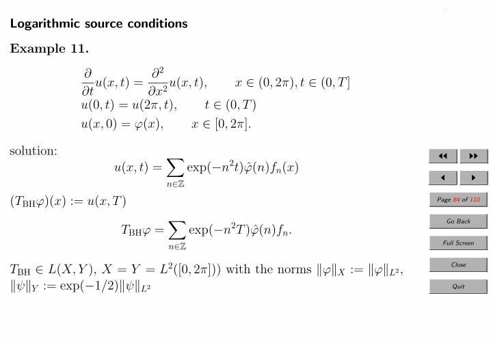
Logarithmic source conditions

Example 11.

∂

∂tu(x, t) =

∂2

∂x2u(x, t), x ∈ (0, 2π), t ∈ (0, T ]

u(0, t) = u(2π, t), t ∈ (0, T )

u(x, 0) = ϕ(x), x ∈ [0, 2π].

solution:u(x, t) =

∑n∈Z

exp(−n2t)ϕ(n)fn(x)

(TBHϕ)(x) := u(x, T )

TBHϕ =∑n∈Z

exp(−n2T )ϕ(n)fn.

TBH ∈ L(X, Y ), X = Y = L2([0, 2π])) with the norms ‖ϕ‖X := ‖ϕ‖L2,‖ψ‖Y := exp(−1/2)‖ψ‖L2

JJ II

J I

of 110

Go Back

Full Screen

Close

Quit

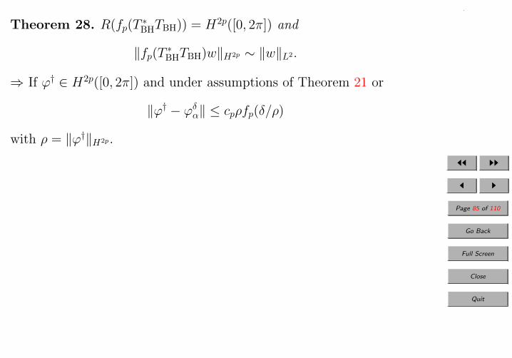
Theorem 28. R(fp(T∗BHTBH)) = H2p([0, 2π]) and

‖fp(T∗BHTBH)w‖H2p ∼ ‖w‖L2.

⇒ If ϕ† ∈ H2p([0, 2π]) and under assumptions of Theorem 21 or

‖ϕ† − ϕδα‖ ≤ cpρfp(δ/ρ)

with ρ = ‖ϕ†‖H2p.

JJ II

J I

of 110

Go Back

Full Screen

Close

Quit

6. Nonlinear operators

6.1. Frechet derivative

Definition 11. Let X, Y be normed spaces, and let U be an opensubset of X. A mapping F : U → Y is called Frechet differentiable atϕ ∈ U if there exists a bounded linear operator F ′[ϕ] : X → Y suchthat

‖F (ϕ+ h)− F (ϕ)− F ′[ϕ]h‖ = o (‖h‖) (2)

uniformly as ‖h‖ → 0. F ′[ϕ] is called the Frechet derivative of F at ϕ.F is called Frechet differentiable if it is Frechet differentiable at everypoint ϕ ∈ U . F is called continuously differentiable if F is differentiableand if F ′ : U → L(X, Y ) is continuous.

JJ II

J I

of 110

Go Back

Full Screen

Close

Quit

Theorem 29. Let F : U ⊂ X → Y be Frechet differentiable, and letZ be a normed space.

1. The Frechet derivative of F is uniquely determined.

2. If G : U → Y is Frechet differentiable, then αF + βG is differen-tiable for all α, β ∈ R (or C) and

(αF + βG)′[ϕ] = αF ′[ϕ] + βG′[ϕ], ϕ ∈ U.

3. (Chain rule) If G : Y → Z is Frechet differentiable, the G F :U → Z if Frechet differentiable, and

(G F )′[ϕ] = G′[F (ϕ)]F ′, ϕ ∈ U.

4. (Product rule) A bounded bilinear mapping b : X × Y → Z isFrechet differentiable, and

b′[(ϕ1, ϕ2)](h1, h2) = b(ϕ1, h2) + b(h1, ϕ2)

for all ϕ1, h1 ∈ X and ϕ2, h2 ∈ Y .

JJ II

J I

of 110

Go Back

Full Screen

Close

Quit

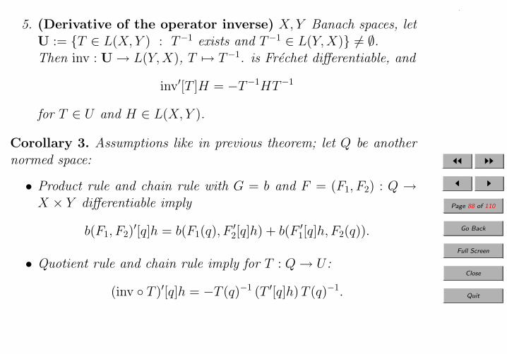
5. (Derivative of the operator inverse) X, Y Banach spaces, letU := T ∈ L(X, Y ) : T−1 exists and T−1 ∈ L(Y,X) 6= ∅.Then inv : U → L(Y,X), T 7→ T−1. is Frechet differentiable, and

inv′[T ]H = −T−1HT−1

for T ∈ U and H ∈ L(X, Y ).

Corollary 3. Assumptions like in previous theorem; let Q be anothernormed space:

• Product rule and chain rule with G = b and F = (F1, F2) : Q →X × Y differentiable imply

b(F1, F2)′[q]h = b(F1(q), F

′2[q]h) + b(F ′

1[q]h, F2(q)).

• Quotient rule and chain rule imply for T : Q→ U :

(inv T )′[q]h = −T (q)−1 (T ′[q]h)T (q)−1.

JJ II

J I

of 110

Go Back

Full Screen

Close

Quit

Definition 12. X Hilbert space, [a, b] ⊂ R bounded interval,G : [a, b] → X continuous.L : X → R (or L : X → C if X complex Hilbert space)

L(ψ) :=

∫ b

a

〈G(t), ψ〉 dt .

L ∈ L(X,R); Riesz representation theorem⇒ exitence of unique l ∈ X:

〈l, ψ〉 = L(ψ)

for all ψ ∈ X. Set ∫ b

a

G(t) dt := l .

It immediately follows that

‖∫ b

a

G(t) dt‖ ≤∫ b

a

‖G(t)‖ dt.

JJ II

J I

of 110

Go Back

Full Screen

Close

Quit

Lemma 13. Let X, Y be Hilbert spaces and U ⊂ X open. Moreover,let ϕ ∈ U and h ∈ X such that ϕ + th ∈ U for all 0 ≤ t ≤ 1. IfF : U → Y is Frechet differentiable, then

F (ϕ+ h)− F (ϕ) =

∫ 1

0F ′[ϕ+ th]h dt.

Lemma 14. Let X, Y be Hilbert spaces and U ⊂ X open. Let F : U →Y be Frechet differentiable and assume that there exists a Lipschitzconstant L such that

‖F ′[ϕ]− F ′[ψ]‖ ≤ L‖ϕ− ψ‖

for all ϕ, ψ ∈ U . If ϕ + th ∈ U for all t ∈ [0, 1], then (2) can beimproved to

‖F (ϕ+ h)− F (ϕ)− F ′[ϕ]h‖ ≤ L

2‖h‖2.

JJ II

J I

of 110

Go Back

Full Screen

Close

Quit

Compactness

Definition 13. Let X, Y be normed spaces, and let U be a subset ofX. An operator F : U → Y is called compact if it maps bounded setsto relatively compact sets. It is called completely continuous if it iscontinuous and compact.

nonlinear case: compactness 6⇒ continuity!

Z another normed space, G : U → Z and H : Z → Y , F = H G:

G compact and H continuous ⇒ F compact

G maps bounded sets to bounded sets and H compact ⇒ F compact

Theorem 30. Let X, Y be normed spaces, and let U ⊂ X be open. IfF : U → Y is compact and X is infinite dimensional, then F−1 cannotbe continuous, i.e. the equation F (ϕ) = g is ill-posed.

Theorem 31. Let X be a normed space, Y a Banach space, and letU ⊂ X be open. If F : U → Y is completely continuous and Frechetdiffentiable, then F ′[ϕ] is compact for all ϕ ∈ U .

JJ II

J I

of 110

Go Back

Full Screen

Close

Quit

6.2. The inhomogeneous medium scattering problem

Determine refractive index of a medium from measurements of far fieldpatterns of scattered time-harmonic acoustic waves in this medium.ui. . . incident field satisfying Helmholtz equation ∆ui + k2ui = 0,e.g. ui(x) = exp(−ikx · θ) with θ ∈ Sd−1 := x ∈ Rd : |x| = 1.Total field

u = ui + us

satisfies inhomogeneous Helmholtz equation

∆u+ k2nu = 0, x ∈ Rd,

and Sommerfeld radiation condition

limr→∞

r(d−1)/2(∂us

∂r− ikus

)= 0, uniformly for all x =

x

|x|.

k > 0. . . wave number, us. . . the scattered field.n = n(x). . . refractive index, Ren ≥ 0, Imn ≥ 0 (absorbing media)n = 1− a with supp a ⊂ Bρ := x ∈ R3 : |x| ≤ ρ for some ρ > 0.

JJ II

J I

of 110

Go Back

Full Screen

Close

Quit

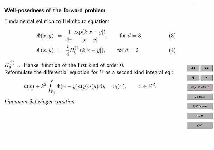
Well-posedness of the forward problem

Fundamental solution to Helmholtz equation:

Φ(x, y) =1

4π

exp(k|x− y|)|x− y|

, for d = 3, (3)

Φ(x, y) =i

4H

(1)0 (k|x− y|), for d = 2 (4)

H(1)0 . . . Hankel function of the first kind of order 0.

Reformulate the differential equation for U as a second kind integral eq.:

u(x) + k2∫

Bρ

Φ(x− y)a(y)u(y) dy = ui(x), x ∈ Rd.

Lippmann-Schwinger equation.

JJ II

J I

of 110

Go Back

Full Screen

Close

Quit

Theorem 32. Assume that a ∈ C1(Rd) satisfies supp a ⊂ Bρ. Thenany solution u ∈ C2(Rd) to(*) the inhomogeneous Helmholtz eq. with Sommerfeld rad. cond.satisfies(**) the Lippmann Schwinger equation.

Vice versa, let u ∈ C(Bρ) be a solution to (**). Then

us(x) := −k2∫

Bρ

Φ(x− y)a(y)u(y) dy, x ∈ Rd

belongs to C2(Rd) and satisfies (*).

Green’s representation formula: for all v ∈ C2(Bρ) ∩ C1(Bρ):

v(x) =

∫∂Bρ

∂v

∂ν(y)Φ(x, y)− v(y)

∂Φ(x, y)

∂ν(y)

ds(y)

−∫

Bρ

∆v(y) + k2v(y)

Φ(x, y) dy, x ∈ Bρ

ν. . . outer normal vector on ∂Bρ

JJ II

J I

of 110

Go Back

Full Screen

Close

Quit

Volume potential V :

(V ϕ)(x) :=

∫Rd

Φ(x, y)ϕ(y) dy, x ∈ Rd.

Theorem 33. Let suppϕ ⊂ Bρ. If ϕ ∈ C(Rd), then V ϕ ∈ C1(Rd),and if ϕ ∈ C1(Rd), then V ϕ ∈ C2(Rd). In the latter case

(∆ + k2)(V ϕ) = −ϕ .

Proof of Theorem 32. Let u ∈ C2(Rd) solve the PDE (*), and let x ∈ Bρ.Green’s formula with v = u and ∆u+ k2u = k2au ⇒

u(x) =

∫∂Bρ

∂u

∂ν(y)Φ(x, y)− u(y)

∂Φ(x, y)

∂ν(y)

ds(y)−k2

∫Bρ

Φ(x, y)a(y)u(y) dy

(5)Green’s formula with v = ui ⇒

ui(x) =

∫Bρ

∂ui

∂νΦ(x, y)− ui(y)

∂Φ(x, y)

∂ν(y)

ds(y). (6)

JJ II

J I

of 110

Go Back

Full Screen

Close

Quit

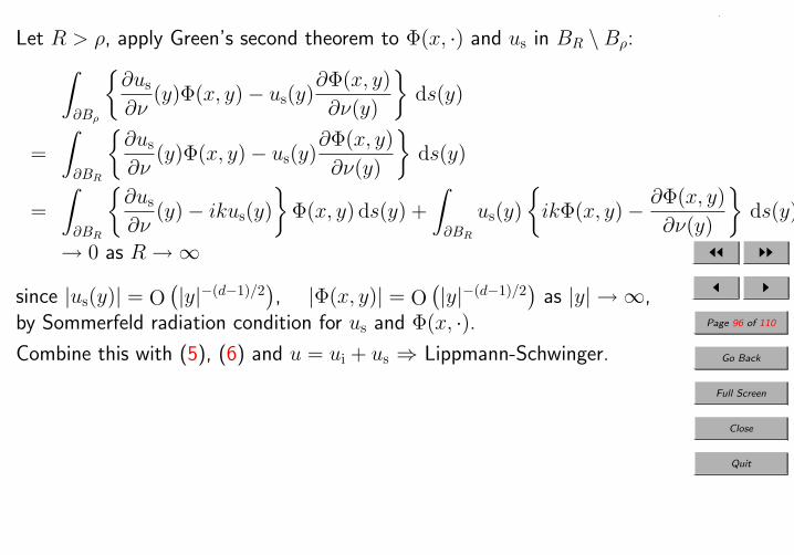
Let R > ρ, apply Green’s second theorem to Φ(x, ·) and us in BR \Bρ:∫∂Bρ

∂us

∂ν(y)Φ(x, y)− us(y)

∂Φ(x, y)

∂ν(y)

ds(y)

=

∫∂BR

∂us

∂ν(y)Φ(x, y)− us(y)

∂Φ(x, y)

∂ν(y)

ds(y)

=

∫∂BR

∂us

∂ν(y)− ikus(y)

Φ(x, y) ds(y) +

∫∂BR

us(y)

ikΦ(x, y)− ∂Φ(x, y)

∂ν(y)

ds(y)

→ 0 as R→∞

since |us(y)| = O(|y|−(d−1)/2

), |Φ(x, y)| = O

(|y|−(d−1)/2

)as |y| → ∞,

by Sommerfeld radiation condition for us and Φ(x, ·).Combine this with (5), (6) and u = ui + us ⇒ Lippmann-Schwinger.

JJ II

J I

of 110

Go Back

Full Screen

Close

Quit

Let u ∈ C(Bρ) solve (**).Φ(·, y) satisfies Sommerfeld radiation condition uniformly for y ∈ Bρ

⇒ us(x) := −k2∫

BρΦ(x− y)a(y)u(y) dy, satisfies Sommerfeld rad.

Theorem 33 ⇒ us ∈ C1(Rd) and

∆us + k2us − k2au = 0 ,

hence even us ∈ C2(Rd).Since ∆ui + k2ui = 0, u = us + ui satisfies inhom. Helmholtz eq.(*)

Theorem 34. The Lippmann-Schwinger equation has a unique solu-tion u ∈ C(Bρ) if ‖a‖∞ < (k2‖V ‖∞)−1.

Proof. Multiplication operator Ma : C(Bρ) → C(Bρ), Mav := av.Smallness assumption on a ⇒ ‖k2VMa‖∞ < 1⇒ I + k2VMa boundedly invertible (Neumann series). Existence possible also without smallness of a by Riesz theory.Uniqueness nontrivial.

JJ II

J I

of 110

Go Back

Full Screen

Close

Quit

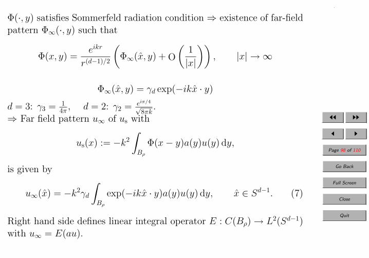
Φ(·, y) satisfies Sommerfeld radiation condition ⇒ existence of far-fieldpattern Φ∞(·, y) such that

Φ(x, y) =eikr

r(d−1)/2

(Φ∞(x, y) + O

(1

|x|

)), |x| → ∞

Φ∞(x, y) = γd exp(−ikx · y)

d = 3: γ3 = 14π , d = 2: γ2 = eiπ/4

√8πk

.⇒ Far field pattern u∞ of us with

us(x) := −k2∫

Bρ

Φ(x− y)a(y)u(y) dy,

is given by

u∞(x) = −k2γd

∫Bρ

exp(−ikx · y)a(y)u(y) dy, x ∈ Sd−1. (7)

Right hand side defines linear integral operator E : C(Bρ) → L2(Sd−1)with u∞ = E(au).

JJ II

J I

of 110

Go Back

Full Screen

Close

Quit

The inverse Problem

Recover a from measurements of u∞.

To uniquely determine function a of d variablesfrom function u∞ of d− 1 variables,consider incident fields ui(x) = ui(x, θ) = exp(ikθ · x) for all θ ∈ Sd−1

→ u(x, θ), us(x, θ), u∞(x, θ).

Forward operator FIM : D(FIM) ⊂ C1c (Bρ) → L2(Sd−1 × Sd−1)

(FIM(a))(x, θ) := u∞(x, θ), x, θ ∈ Sd−1 (8)

C1c (Bρ). . . space of all continuously differentiable functions on Bρ with

supp a ⊂ Bρ

D(FIM) := a ∈ C1c (Bρ) : Re(1− a) ≥ 0, Im(a) ≤ 0.

Identifiability: FIM is one-to-one (Colton, Kress, Kirsch, Hahner)

JJ II

J I

of 110

Go Back

Full Screen

Close

Quit

Frechet diffrentiability of FIM:

Theorem 35. 1. The operator G : D(FIM) → C(Rd×Sd−1), G(a) :=u, is Frechet differentiable with respect to the supremum norm onD(FIM), and u′ := G′[a]h satisfies the integral equation

u′ + k2V (au′) = −k2V (hu) (9)

for all a ∈ D(FIM) and h ∈ C1c (Bρ).

2. FIM is Frechet differentiable with respect to the maximum norm onD(FIM).

Proof. 1) D(FIM) → L(C(Bρ × Sd−1)), a 7→ Ma where (Mav)(x, θ) :=a(x)v(x, θ) is linear and bounded wrt supremum norm, hence Frechetdifferentiable.Chain rule and quotient rule ⇒ D(FIM) → L(C(Bρ × Sd−1)), a 7→(I + k2VMa)

−1 Frechet-differentiable.Chain rule ⇒ G(a) = (I + k2VMa)

−1ui Frechet-differentiable.Differentiate both sides of Lippmann-Schwinger equation wrt a, use theproduct rule ⇒ (9).

JJ II

J I

of 110

Go Back

Full Screen

Close

Quit

2) follows from 1) by F (a) = E(MaG(a)), with product and the chainrule.

JJ II

J I

of 110

Go Back

Full Screen

Close

Quit

7. Nonlinear Tikhonov regularization

X, Y be Hilbert spaces, F : D(F ) ⊂ X → Y continuous operator.

F (ϕ) = g (10)

‖gδ − g‖ ≤ δ, ϕ† . . . exact solution, ϕ0. . . initial guess.

Nonlinear Tikhonov regularization:

‖F (ϕ)− gδ‖2 + α‖ϕ− ϕ0‖2 = minϕ∈D(F )

!

Tikhonov functional: Jα(ϕ) = (‖F (ϕ)− gδ‖2 + α‖ϕ− ϕ0‖2

Variants:

• different regularization term

• minimization over closed convex subset of D(F ) (constraints).

JJ II

J I

of 110

Go Back

Full Screen

Close

Quit

7.1. Preliminaries on weak convergence in Hilbert spaces

Definition 14. X Hilbert space (ϕn) ⊂ X, converges weakly to ϕ ∈ X

ϕn ϕ as n→∞

if∀ψ ∈ X : 〈ϕn, ψ〉 → 〈ϕ, ψ〉 , n→∞

A weak limit of a sequence is uniquely determined.

Strong convergence implies weak convergence.

Weak convergence does not imply strong convergence.(counterexample: ONS in X)

Lemma 15. If T ∈ L(X, Y ), then T is weakly continuous, i.e. ϕn ϕimplies Tϕn Tϕ as n→∞.

Lemma 16. If ϕn ϕ, then lim supn→∞ ‖ϕn‖ ≥ ‖ϕ‖, i.e. the norm isweakly lower semicontinuous.

Theorem 36. Every bounded sequence has a weakly convergent subse-quence.

JJ II

J I

of 110

Go Back

Full Screen

Close

Quit

Definition 15. .A subset K of a Hilbert space X is called weakly closed if it containsthe weak limits of all weakly convergent sequences contained in K, i.e.

∀(ϕn)n∈N ⊆ K : (ϕn ϕ) ⇒ (ϕ ∈ X)

An operator F : D(F ) ⊂ X → Y is called weakly closed if its graphgrF := (ϕ, F (ϕ)) : ϕ ∈ D(F ) is weakly closed in X × Y , i.e. if

∀(ϕn)n∈N ⊆ D(F ) :

(ϕn ϕ and F (ϕn) g) ⇒ (ϕ ∈ D(F ) and F (ϕ) = g)

F weakly continuous and D(F ) weakly closed ⇒ F weakly closed.

Theorem 37. If K ⊂ X is convex and closed, then K is weakly closed.

JJ II

J I

of 110

Go Back

Full Screen

Close

Quit

7.2. Convergence analysis of Tikhonov reguarization

Theorem 38. (Existence of global minimizer)Assume that F is weakly closed. Then for all α > 0, the Tikhonovfunctional has a global minimizer ϕδ

α.

This minimizer is not necessarily unique!

Theorem 39. (Stability)Assume that F is weakly closed. Let α > 0, and denote for a sequencegk, by ϕk the sequence of minimizers of ‖F (ϕ) − gk‖2 + α‖ϕ − ϕ0‖2.Then for any sequence gk → gδ, there exists a convergent subsequenceof ϕk and the limit of each convergent subsequence of ϕk is a minimizerof ‖F (ϕ)− gδ‖2 + α‖ϕ− ϕ0‖2. (“ϕk converges subsequentially”).

JJ II

J I

of 110

Go Back

Full Screen

Close

Quit

Theorem 40. (Convergence) Assume that F is weakly closed and letα = α(δ) be chosen such that

α(δ) → 0 andδ2

α(δ)→ 0 as δ → 0.

Let gδk be some sequence in Y such that ‖gδk − g‖ ≤ δk and δkk→∞→ 0.

Then ϕδkαk

converges subsequentially to a solution to F (ϕ) = g. If, inaddition, a solution ϕ† to F (ϕ) = g is unique, then

‖ϕδkαk− ϕ†‖ → 0 as k →∞.

JJ II

J I

of 110

Go Back

Full Screen

Close

Quit

Convergence rates under source conditions

ϕ† − ϕ0 = (F ′[ϕ†]∗F ′[ϕ†])µw, L‖w‖ < 1

for some w ∈ X with ‖w‖ sufficiently small.

Case µ = 12 :

Theorem 41. (Convergence rates)Assume that F is weakly closed and Frechet differentiable, that D(F )is convex, and that F ′ is Lipschitz with constant L.Moreover, assume that the source condition

ϕ† − ϕ0 = F ′[ϕ†]∗w,

L‖w‖ < 1

is satisfied for some w ∈ Y and that a parameter choice rule

α = cδ

with some c > 0 is used. Then there exists a constant C > 0 indepen-dent of δ such that

‖ϕδα − ϕ†‖ ≤ C

√δ,

‖F (ϕδα)− g‖ ≤ Cδ.

JJ II

J I

of 110

Go Back

Full Screen

Close

Quit

Problem: Find a global minimizer of the Tikhonov functional:

Definition 16. Let C ba a closed convex subset of the Hilbert spaceX.

(minα

) Jα(ϕ) = minφ∈C

!

is called quadratically well posed if there exists an open neighborhoodV of F (C) such that for every gδ ∈ V

• (minα) has a unique solution φδα;

• (minα) has no additional local minima;

• any minimizing sequence converges to φδα;

• the mapping gδ 7→ φδα is locally Lipschitz continuous from V ⊆ X

to C ⊆ Y .

JJ II

J I

of 110

Go Back

Full Screen

Close

Quit

Theorem 42. Let for any path

P : t ∈ [0, 1] 7→ F ((1− t)ϕ0 + tϕ1)

with ϕ0, ϕ1 ∈ C with velocity V and acceleration A according to

V (t) = P ′(t), A(t) = P ′′(t)

the following assumptions hold:

P ∈ W 2,∞([0, 1]) for all pairs ϕ0, ϕ1 ∈ C ,

∃M > 0, R > 0 ∀ϕ0, ϕ1 ∈ C, t ∈ [0, 1] :

‖V (t)‖ ≤M‖ϕ0 − ϕ1‖ ‖A(t)‖ ≤ 1

R‖V (t)‖2 (F weakly nonlinear)

Mdiam(C) < πR (size × curvature condition.)

Then there exists an α > 0 such that for all α ≤ α,

(minα

) is quadratically well posed.

JJ II

J I

of 110

Go Back

Full Screen

Close

Quit

Literature on nonlinear Tikhonov regularization:

Seidman, Vogel, 1989: ConvergenceEngl, Kunisch, Neubauer, 1989: Convergence rates for µ = 1

2Neubauer, 1989, Hofmann, Scherzer 1996: Conv. rates for µ ∈ [0, 1]Scherzer, Engl, Kunisch, 1993: a posteriori parameter choice rulesChavent, Kunisch 1996: quadratic well posedness if weakly nonlinear.

inverse probleme jj ii einleitung algoritms for · direct problem, while the latter is called the...

Documents