DIPLOMARBEIT

Titel der Diplomarbeit

„Solution Methods for Lot-Sizing Problems – Multi-Level Models with and without Linked Lots“

Verfasser

Wolfgang Summerauer

angestrebter akademischer Grad

Magister der Sozial- und Wirtschaftswissenschaften (Mag. rer. soc. oec.)

Wien, im November 2008 Studienkennzahl lt. Studienblatt: A 157

Studienrichtung lt. Studienblatt: Internationale Betriebswirtschaft

Erster Betreuer: O. Univ.-Prof. Dipl.-Ing. Dr. Richard F. Hartl

Zweiter Betreuer: Univ.Ass. Dipl.-Ing. Dr. Christian Almeder

Contents

1 Introduction 3

2 The Lot-Sizing Problem 52.1 Uncapacitated Lot-Sizing Problem . . . . . . . . . . . . . . . . . . . . . . 52.2 Capacitated Lot-Sizing Problem . . . . . . . . . . . . . . . . . . . . . . . 62.3 Multi-Level Problems . . . . . . . . . . . . . . . . . . . . . . . . . . . . . 62.4 Small- and Big-Bucket Models . . . . . . . . . . . . . . . . . . . . . . . . 62.5 Solution Approaches . . . . . . . . . . . . . . . . . . . . . . . . . . . . . 8

3 Mathematical Formulation 103.1 Standard Formulation . . . . . . . . . . . . . . . . . . . . . . . . . . . . 103.2 Simple Plant Location Formulation . . . . . . . . . . . . . . . . . . . . . 12

4 Decomposition 144.1 Standard Formulation . . . . . . . . . . . . . . . . . . . . . . . . . . . . 144.2 Simple Plant Location Formulation . . . . . . . . . . . . . . . . . . . . . 20

5 Ant Colony Algorithm 215.1 General Description . . . . . . . . . . . . . . . . . . . . . . . . . . . . . . 215.2 MAX-MIN Ant System for the MLCLS problem . . . . . . . . . . . . . . 22

6 Results for the MLCLS Problem 266.1 Computational Results . . . . . . . . . . . . . . . . . . . . . . . . . . . . 266.2 Criticism . . . . . . . . . . . . . . . . . . . . . . . . . . . . . . . . . . . . 28

7 Solution Approach for the Linkage Property 307.1 Model Formulation . . . . . . . . . . . . . . . . . . . . . . . . . . . . . . 307.2 Decomposition . . . . . . . . . . . . . . . . . . . . . . . . . . . . . . . . 32

8 Results for the CLSPL 35

9 Conclusion 37

Bibliography 38

A Detailed Results 42

1 Introduction

In this thesis we center our attention on the lot sizing problem, which is part of thematerial requirements planning (MRP). In many production processes it costs moneyand takes time to setup a machine for a certain product. A lot-sizing problem there-fore identifies the optimal timing and batch size of production. More precisely, it triesto minimize the inventory, setup, and production costs while meeting the required de-mand. Since production decisions and costs directly affect a company’s efficiency andcompetitiveness in the market, the lot sizing problem is of utmost importance for everyproducing firm.

There are many different models and methods for solving various lot sizing problems.This thesis mainly deals with the multi-level capacitated lot-sizing problem (MLCLS),and then expands the model by adding the possibility of linking a setup state fromone period to the next. The MLCLS problem is NP-complete (see Maes and McClain,1991, for a proof). The solution approach used for the MLCLS problems is a hybridalgorithm from Pitakaso et al. (2006) which decomposes the given problem into multiplesmaller subproblems. These subproblems are then solved by CPLEX, a commercialLP/MIP-Solver developed by ILOG. An Ant Colony Optimization (ACO) algorithm, aprobabilistic metaheuristic that mimics the behavior of ants, is then applied to determinethe lot-sizing sequence and to improve the decomposition. The ACO algorithm used inthis thesis is a MAX-MIN ant system (MMAS) developed by Stützle and Hoos (1997).Our approach works very well with medium-sized problems, but is not able to competewith the other approaches when solving large-sized test instances.

As stated before, the capacitated lot-sizing problem is then expanded by adding alinkage property to the model. We use the same ant-based approach to solve the capac-itated lot-sizing problem with linked lot sizes (CLSPL) which combines the characteris-tics of big- and small-bucket models. The CLSPL is a big-bucket model that allows thepreservation of a setup state from one period to the next. We implement the CLSPLformulation suggested by Stadtler and Suerie (2003). Since this CLSPL model exchangesthe common production variable by a simple plant location (SPL) formulation, we alsotest these two formulations for effectiveness. Our approach to solve the CLSPL problemis then tested with single-level and multi-level test instances.

The remainder of this thesis is organized as follows. Section 2 provides a detailedliterature review of the different lot-sizing problems. Furthermore, an overview of thesolution approaches for the lot-sizing problem is given. In the third Section the math-

3

ematical formulation is defined while the fourth Section explains the decomposition.Section 5 describes the MMAS algorithm and is followed by computational results forthe MLCLS problem in Section 6. The solution approach for the linkage property isgiven in Section 7. Results for the CLPSL problem are presented in Section 8. Finally,the thesis finishes with a summary and further possible research in Section 9.

4

2 The Lot-Sizing Problem

2.1 Uncapacitated Lot-Sizing Problem

The first formulation of a dynamic lot-sizing problem dates back to Wagner and Whitin(1958) who introduced a single-item uncapacitated lot-sizing problem (ULS). In order tooptimally solve the underlying problem a linear programming (LP) model is required. ALP model tries to optimize a certain objective function subject to some linear constraints.More precisely, the problem below is a mixed integer programming (MIP) model, whichmeans that not all the variables have to be integer. The MIP model is as follows:

minT∑t=1

(styt + htIt + cxt xt), (1)

subject to

It = It−1 + xt − Et, ∀t, (2a)

xt ≤( T∑

τ=t

Et

)yt ∀t, (2b)

It ≥ 0, xt ≥ 0, yt ∈ {0, 1}, ∀t. (2c)

The model contains the following variables: xt stands for the production quantityin period t, yt is the setup variable, and It represents the inventory level in periodt. Therefore, the objective function (1) tries to minimize the overall production(cxt ),inventory(ht), and setup (st) costs. The first constraints (2a) make sure that the externaldemand Et is satisfied by either production in period t or by inventory from previousperiods. Moreover, the constraints determine how much inventory is stored for futuredemands. The second constraints (2b) state that whenever production occurs a setuphas to be made. Finally, the last constraints (2c) are the usual non-negativity and binaryconstraints.

Concerning the multi-item uncapacitated lot-sizing model, Wolsey (1989) for exampleanalyzed the problem with start-up costs, while Pochet and Wolsey (1987) examinedthe problem with backlogging. Other authors for example developed simple heuristicsto minimize the average setup cost and inventory cost over several periods (see Silverand Meal, 1973). Zangwill (1969) showed that the ULS is in effect a fixed charge networkproblem.

5

2.2 Capacitated Lot-Sizing Problem

A classical extension to the basic formulation is the multi-item capacitated lot-sizingproblem (CLSP) (see Figure 1 in Section 2.4) where several items can be produced onone machine within one period over a given planning horizon. Production is thereforelimited by the capacity constraint. The CLSP is NP-hard (see Bitran and Yanasse, 1982,for a proof). Trigeiro et al. (1989) extended the CLSP by adding setup times to themodel.

2.3 Multi-Level Problems

The multi-level lot-sizing (MLLS) model deals with production processes that use varioussubassemblies and components to build a certain end item. Therefore, two kind ofdemands have to be considered in the inventory constraint: the primal (external) demandfrom the market place, and the secondary (internal) demand which is triggered whenthe production process starts to lot-size the ordered end item. Zangwill (1966) startedwith an uncapacitated multi-facility problem while Lambrecht and Vander Eecken (1978)extended the approach by adding capacity constraints at the last level. Further researchfor example was made by McClain and Thomas (1989), Tempelmeier and Helber (1994)and Harrison and Lewis (1996). Authors like e.g. Stadtler (2003) and Tempelmeier andDerstroff (1996) added set up times to the problem.

2.4 Small- and Big-Bucket Models

Another distinction in the literature is between small- and big-bucket models. Big-bucket models have the assumption that several products can be produced on the samemachine in one period, while small-bucket models only allow a setup for one product onthe same machine. However, in a small-bucket model it is possible to carry over a setupstate for a certain item from one period to the next. Fleischmann (1990) proposed thediscrete lot-sizing and scheduling problem (DLSP) where the linking of a setup statefor one item is only possible if production uses the full capacity in the next period. Incontrast, Karmarkar and Schrage (1985) and Salomon (1986) analyzed the continuoussetup lot-sizing problem (CSLP) where production has not to use up the full capacity.The following LP model represents the CSLP formulation:

minP∑i=1

T∑t=1

(sizit + hiIit + cxi xit), (3)

6

subject to

Iit = Iit−1 + xit − Eit, ∀i, t, (4a)P∑i=1

yit ≤ 1 ∀t, (4b)

aixit ≤ Ltyit ∀i, t, (4c)

zit ≥ yit − yit−1 ∀i, t, (4d)

Iit ≥ 0, xit ≥ 0, yit, zit ∈ {0, 1}, ∀i, t. (4e)

The objective function (3) includes a new variable called start up variable zit. Everytime a machine is set up for which it was not set up in the previous period start up costssi occur. There is no change to the inventory constraints (4a). Constraints (4b) limitthe setup per item and period to one. The next constraints (4c) restrain the productionquantity by the available capacity Lt if a setup is made in that period. Constraints (4d)state that an item can only start up if the setup for that item in the current period isnot equal to the setup in the previous period. The last constraints (4e) are again theusual binary and non-negativity constraints.

Note that the only difference between the DLSP and the CSLP is that in the DLSPconstraints (3c) are formulated as an equality. Furthermore, the proportional lot sizingand scheduling problem (PLSP, see Figure 1) allows two items per period to use the samecapacity, whereas there is no restriction concerning the consumption of the capacity (cf.Drexl and Haase, 1995.

Although the small-bucket model represents a more realistic scenario and allows formore accurate planning, it is certainly undesirable to divide the planning horizon into ahuge number of small periods since it increases the complexity for the solution approach.To avoid the mentioned weakness of the small-bucket model and the possibly unrealisticsimplifications of the big-bucket model, new model formulations are presented in theliterature to combine both models. Fleischmann and Meyr (1997) introduced the generallot-sizing and scheduling problem (GLSP) where large time periods can be divided intoseveral smaller time buckets of variable length, and the production in these periods isrestricted to a single item. The model formulation we use in this thesis is the capacitatedlot-sizing problem with linked lot sizes (CLSPL)(see e.g. Gopalakrishnan et al., 1995,2001; Haase, 1994; Sox and Gao, 1999; Stadtler and Suerie, 2003) which is a big-bucketmodel that allows to carry-over setup states (see Figure 1).

7

Figure 1: Three different formulations of the lot-sizing problem with linked lot sizes.The Figure is taken from Stadtler and Suerie (2003).

2.5 Solution Approaches

The lot-sizing problem is well known for being hard to solve, since even the single-itemcapacitated problem is NP-hard (see Florian et al., 1980, for a proof). For that reason alot of research has been published on how to solve the problem efficiently in an alternativeway. Since some formulations for the (mixed) integer programming problem yield totighter bounds, various authors proposed strong valid inequalities and/or different modelformulations. Tempelmeier and Helber (1994) analyzed a network or shortest pathformulation, while Stadtler (1996) proposed a simple plant location formulation. Othercontributions include heuristic algorithms with or without decomposition (e.g. Almada-Lobo et al., 2007; Stadtler and Suerie, 2003; Tempelmeier and Derstroff, 1996).

More recently, the use of metaheuristic became a well-established way of solving theunderlying lot-sizing problem, such as the genetic algorithm (GA), simulated annealing(SA), tabu search (TS), and ant colony optimization (ACO). Xie and Dong (2002) useda GA, which belongs to the evolutionary algorithms and is based on the ideas of naturalselection and genetics, to solve the CLSP. Furthermore, Dellaert and Jeunet (2000) solvedthe uncapacitated MLLS problem with a GA. Berretta and Rodrigues (2004) proposeda memetic algorithm, which is a less constrainted method of the GA, to solve multi-levelcapacitated lot-sizing problems. Their reported results for the small-sized instances couldimprove the solutions obtained by Tempelmeier and Derstroff (1996). Oezdamar and

8

Barbarosoglu (2000) proposed a Lagrangean relaxation-simulated annealing approachfor the multi-level capacitated lot-sizing problem. SA is a metaheuristic which comesfrom annealing in metallurgy, and it is based on the heating and cooling of some material.The controlled slow cooling of the material allows the molecules to have enough timeto restructure and build stabilized crystals with lower internal energy. Oezdamar andBarbarosoglu (2000) could improve the results for the small-sized instances obtained byTempelmeier and Derstroff (1996) but not reach the results from Berretta and Rodrigues(2004). TS is a technique which uses memory structures to set potential solution ’taboo’so that this solution can not be visited again. Kimms (1996) for example used the TSto solve multi-level lot-sizing and scheduling problems. The ACO algorithm is basedon the behavior of ants, which when searching for nourishment, walk randomly untilthey find some food, leaving pheromone trails behind. Authors like Pitakaso et al.(2006) and Almeder (2007) proposed ant-based algorithms to solve multi-item multi-level capacitated lot-sizing problems. Their approaches were tested with the instancesprovided by Tempelmeier and Derstroff (1996). Almeder (2007) delivers by far the bestresults for the medium-ranged instances, while the approach of Pitakaso et al. (2006) issuperior to all the other approaches for the large-sized test instances. The time-orienteddecomposition heuristic from Stadtler (2003) also provides very good results for thelarge-sized instances.

9

3 Mathematical Formulation

3.1 Standard Formulation

This Section provides a mathematical formulation for the MLCLS problem which orig-inates from Stadtler (1996) and was used by Pitakaso et al. (2006). The indices, pa-rameters and decision variables as well as the model itself are taken from Pitakaso et al.(2006).

Dimensions and indices:

P number of products in the bill of materialT planning horizonM number of resourcesi item index in the bill of materialt period indexm resource index

Parameters:

Γ(i) set of immediate successors of item i

Γ−1(i) set of immediate predecessors of item i

si setup cost for item i

cij quantity of item i required to produce unit of item j

hi holding cost for item i

ami capacity needed on resource m for one unit of item i

bmi setup time for item i on resource mLmt available capacity for resource m in period tcom overtime cost of resource mG sufficiently large numberhi holding cost for item i

Eit external demand for product i in period tIi0 initial inventory of item i

10

Decision variables:

xit delivered quantity of item i at the beginning of period tIit inventory level of item i at the end of period tOmt overtime hours used on resource m in period tyit binary variable indicating whether item i is produced in period t (yit = 1)

or not (yit = 0)

minP∑i=1

T∑t=1

(siyit + hiIit) +T∑t=1

M∑m=1

comOmt, (5)

subject to

Iit = Iit−1 + xit −∑j∈Γ(i)

cijxjt − Eit, ∀i, t, (6a)

P∑i=1

(amixit + bmiyit) ≤ Lmt +Omt, ∀m, t (6b)

xit −Gyit ≤ 0, ∀i, t, (6c)

Iit ≥ 0, Omt ≥ 0, xit ≥ 0, yit ∈ {0, 1}, ∀i, t. (6d)

The objective function (5) intends to minimize the total setup costs, holding costsand overtime costs. So whenever the available capacity is not sufficient, overtime maybe used to meet the dynamic demand. The first equation (6a) in the model is theinventory balance equation, which assures that the inventory level of item i in period tis equal to the sum of the inventory level of the previous period, the amount produced inperiod t minus the internal demand needed to produce item i and the external demand.Constraints (6b) ensure that the available capacity and the overtime hours used are notexceeded by the capacity used for production and setup. Whereas constraints (6c) statethat production in any period t for a certain item i is only possible if a setup is made inthat period, with G representing the sum of the remaining demand. Due to performancereasons it is recommended to use a small value of G. The last constraints (6d) are thecommon non-negativity and binary constraints.

11

3.2 Simple Plant Location Formulation

The SPL formulation has been used by several authors to solve various lot-sizing prob-lems. It was first introduced by Krarup and Bilde (1977) and then e.g. used by Rosling(1986) for assembly product structures and then considered by Maes and McClain (1991)for serial product structures. Here, we utilize the formulation proposed by Stadtler(1996) and Stadtler and Suerie (2003).

To properly implement the SPL formulation a few changes have to be considered inthe LP model. First, the production variables xit are exchanged by zist respective to

xit :=T∑s=t

Dniszits, ∀i, t. (7)

The three-index production variable zits can be seen as the portion of demand of itemi produced for period s in period t. So basically a certain item i can only be produced ifa ’plant location’ has been made in period t for the present period or for any followingperiod s. Dn

is represents the net demand of product i in period t and it is calculatedaccording to Stadtler (1996):

1, . . . , P : δ = Ii0[1, . . . , T : Dn

it = max

{0, Eit +

i−1∑j=1

cijDnjt − δ

},

δ = max

{0, δ − Eit −

i−1∑j=1

cijDnjt

}.

] (8)

So Dnit is either zero or the sum of the external and internal demand of item i in period

t minus δ, which represents the remaining inventory at the beginning of period t.

The revised mixed-integer model formulation is identical to the model from Stadtlerand Suerie (2003), except for the fact that the model below allows for overtime.

minP∑i=1

T−1∑s=1

T∑t=s

hi(t− s)zistDnit +

P∑i=1

T∑t=1

siyit +T∑t=1

M∑m=1

comOmt (9)

12

subject to

Iit = Iit−1 +T∑s=t

zitsDnis −

∑j∈Γ(i)

T∑s=t

cijzjtsDnjs − Eit, ∀i, t, (10a)

P∑i=1

T∑s=t

amizitsDnis +

P∑i=1

bmiyit ≤ Lmt +Omt, ∀m, t, (10b)

zits ≤ yit, ∀i, t, s = t, . . . , T, (10c)t∑

s=1

zist = 1, ∀i, t,Dnit > 0, (10d)

Iit ≥ 0, Omt ≥ 0, yit ∈ {0, 1}, zist ≥ 0, ∀i, t, s = t, . . . , T. (10e)

The first change applies to the objective function (9), which now calculates the inven-tory costs by multiplying the holding costs of product i and the portion of demand ofitem i produced in t for s with the time difference between the period indices t and s. Forconstraints (10c), it is now possible to omit the parameter G since production variableszist will never take value above one. A new equation (10d) is needed to ensure that therequired demand in each period is satisfied. As before, constraints (10e) are the typicalnon-negativity and binary constraints which in this case also assure that the variableszist never take values below zero. Concerning the other constraints, the variables xit arereplaced by zist according to (7).

13

4 Decomposition

4.1 Standard Formulation

Since obtaining an optimal solution for a MLCLS problem with real world instances israther time consuming, the problem is divided into various subproblems, which are thensolved exactly. In the absence of a realistic scenario this can be done by constructingsubproblems for either items or periods. But with sizes ranging between 40-100 items inthe bill of materials and 20-40 periods, it can be easily seen that the problem size wouldstill be too big to be solved within a reasonable time. To avoid this flaw, the underlyingapproach combines both variants and splits the bill of material as well as the number ofperiods into several subproblems.

Prior to the decomposition, the items in the bill of material are sorted so that thesuccessors of a certain item are always positioned somewhere before that item in thelist. So if we number the items in the list from 1 to P and item i is a direct successorof item j, then i < j. This lot-sizing sequence allows us to schedule the products oneafter another, which can lead to numerous variations in the presence of a general system.Furthermore, it is advisable to introduce an overlap region for items and periods in asubproblem to consider the interdependencies between periods and items in differentsubproblems. Thus, only a certain number of items and periods are fixed after thecomputation of one subproblem.

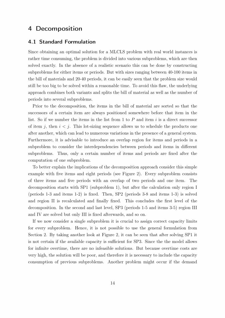
To better explain the implications of the decomposition approach consider this simpleexample with five items and eight periods (see Figure 2). Every subproblem consistsof three items and five periods with an overlap of two periods and one item. Thedecomposition starts with SP1 (subproblem 1), but after the calculation only region I(periods 1-3 and items 1-2) is fixed. Then, SP2 (periods 3-8 and items 1-3) is solvedand region II is recalculated and finally fixed. This concludes the first level of thedecomposition. In the second and last level, SP3 (periods 1-5 and items 3-5) region IIIand IV are solved but only III is fixed afterwards, and so on.

If we now consider a single subproblem it is crucial to assign correct capacity limitsfor every subproblem. Hence, it is not possible to use the general formulation fromSection 2. By taking another look at Figure 2, it can be seen that after solving SP1 itis not certain if the available capacity is sufficient for SP3. Since the the model allowsfor infinite overtime, there are no infeasible solutions. But because overtime costs arevery high, the solution will be poor, and therefore it is necessary to include the capacityconsumption of previous subproblems. Another problem might occur if the demand

14

0 1 2 3 4 5 6 7 80

1

2

3

4

5

SP2

SP3

Periods

Lot

-Siz

ing

Sequ

ence

I

SP1

II

III IV

Figure 2: Every subproblem consists of three items and five periods with an overlap oftwo periods and one item. So after e.g. solving SP1 only region I (periods 1-3and items 1-2) is fixed.

in one subproblem exceeds the available capacity in that time interval while it wouldbe sufficient in previous periods. As a result, the capacity consumption for setup andproduction of an item have to be modified to take the capacity needs of its predecessorsinto account.

This adaption of the problem will lead to additional variables and parameters whichare described below. The notation and the model with its description are again takenfrom Pitakaso et al. (2006).

k index of the subproblemT ks starting time period of subproblem k

T ke last time period of subproblem k

P ks number of first item of subproblem k

P ke number of last item of subproblem k

Akmi modified capacity needed for production of one unit of item i on resource mBkmit modified capacity needed for setup of production of item i in period t on resource m

Skit modified setup cost for item i in period t of subproblem k

Xit lot size for product i in period t (already determined in previous subproblems)Zist lot size for product i in period t produced in period s

(already determined in previous subproblems)Yit binary variable indicating whether item i is scheduled to be produced in period t

15

(already determined in previous subproblems)avCk

mt available regular capacity of resource m in period t for subproblem k

The mixed-integer problem for subproblem k is then

min

Pke∑

i=Pks

Tke∑

t=Tks

(Skityit + hiIit) +

Tke∑

t=Tks

M∑m=1

comOmt, (11)

subject to (each constraint must hold for all i = P ks , . . . , P

ke , t = T ks , . . . , T

ke , and m =

1, . . . ,M)

Iit = Iit−1 + xit −∑j∈Γ(i)j<Pk

s

cijXjt −∑j∈Γ(i)j≥Pk

s

cijxjt − Eit, (12a)

Pke∑

i=Pks

(amixit + bmiyit) ≤ Lmt +Omt −Pk

s −1∑i=1

(amiXit + bmiYit), (12b)

t∑τ=Tk

s

Pke∑

i=Pks

(Akmixiτ +Bkmiτyiτ ) ≤

t∑τ=Tk

s

(avCkmτ +Omτ ), (12c)

xit −Gyit ≤ 0, (12d)

Iit ≥ 0, xit ≥ 0, Omt ≥ 0, yit ∈ {0, 1}. (12e)

Various authors have proposed numerous methods to deal with setup costs whensolving a multi-level lot-sizing problem by a series of single level lot-sizing problems (e.g.Dellaert and Jeunet, 2003; McLaren, 1977). The method used here is a randomizedcumulative Wagner-Whitin (RCWW) method from Pitakaso et al. (2007) which is anextension of Dellaert and Jeunet (2003). The difference between these methods is thatPitakaso et al. (2007) use sequence-dependent time-varying setup costs (STVS), so themodified setup costs for every product depend on the actual position in the productionsequence.

The reason for using modified setup costs in the objective function (11) is due to thefact that lot-sizing an item in a current period results in additional lot-sizes for somepredecessors in previous periods. So the setup costs of an item are adapted by a fractionof the setup costs of all its predecessors. This leads to two cases: (i) the predecessor ofan item already has a positive demand, which results in no additional costs; (ii) there isno positive demand for a predecessor and therefore we have to add the modified setupcosts. To calculate the modified setup cost we introduce a new variable

16

Tijt is a binary variable which equals to 1 if a lot size of item i in period t leads toa positive demand for predecessor j (j ∈ Γ−1(i)) in period t; Tijt equals to 0 if there isalready a planned lot-size for item j in period t (resulting from a different successorof item j).

and calculate the modified setup costs as following:

Skit = si + ri∑

j∈Γ−1(i)j>Pk

e

T (i, j, t)Sj|Γ(j)|

, (13a)

where Sj is calculated recursively by

Si = si +∑

j∈Γ−1(i)

Sj|Γ(j)|

, (13b)

and ri by

ri = R ·(

1 +P − 2Φi + 1

P − 1· u), (13c)

Hence, the value of variable Tijt depends on how the products are scheduled in thelot-sizing sequence. To avoid adding the setup costs for a single item multiple times, themodified setup costs are divided by the immediate successors in the present subprob-lem. This is due to the fact that not every new lot for an item also creates a positivedemand for a certain predecessor if some item with the same predecessor has alreadybeen scheduled. The random variable ri decides how much the setup costs of the prede-cessors influence the modified setup costs. The parameters R ∈ {0, 0.5} and u ∈ {−1, 1}are uniformly distributed random variables, whereas Φi ∈ {1, . . . , P} is the position ofitem i in the lot-sizing sequence. Thus, for the first item (= end item) scheduled inthe lot-sizing sequence we obtain ri = R(1 + u), whereas for the last item we obtainri = R(1− u). Therefore R determines the average value of r over all items and u is theslope.

The inventory balance equation (12a) is slightly modified to consider the productionquantity fixed in some previous subproblems. To ensure that the available capacity issufficient in the current subproblem the right-hand side of capacity constraint (12b) is

17

now reduced by the amount of resources already used in previous subproblems.A cumulative capacity constraint (12c) is introduced to the model which should guar-

antee that the global solution will only use overtime if it is inevitable. The summationterm on the left-hand side contains the accumulated capacity needs for every item in thesubproblem. The idea behind the modified capacity needs Akmi and Bk

mit is that if someitem is scheduled, we also have to consider the resources needed for its predecessors insome previous period. They are calculated recursively as follows:

Akmi = ami +∑

j∈Γ−1(i)j>Pk

e

Akmj, (14)

Bkmit = bmi +

∑j∈Γ−1(i)j>Pk

e

T (i, j, t)B̃mj

|Γ(j) ∩∆(i)|, (15a)

where B̃mj is the accumulated capacity needed for setup of product i on resource m

B̃mi = bmi +∑

j∈Γ−1(i)

B̃mj. (15b)

Note that the concept of equation (15a) is quite similar to the calculation of the time-varying modified setup costs in (13a). The accumulated capacity needed for setup ofproduct i on resource m is divided by the number of immediate successors which arelocated in the same group as item i. There are three groups: (i) already lot-sized items;(ii) items in the present subproblem k; and (iii) items which are not yet scheduled.

∆(i) =

{i, . . . , P k

s − 1}, if i < P ks ,

{P ks , . . . , P

ke }, if P k

s ≤ i ≤ P ke ,

{P ke + 1, . . . , P}, if i > P k

e .

(15c)

The available capacity avCkmt is calculated by subtracting the already used resources

18

and the yet to schedule resource consumption from the total available capacity Lmt.

avCkmt = Lmt −

Pks −1∑i=1

(AkmiXit +BkmitYit)−

P∑i=Pk

e +1

Γ(i)=∅

(AkmiEit +BkmitY

Eit ), (16a)

where

Y Eit =

1, Eit > 0,

0, otherwise.(16b)

Due to the fact that a single subproblem does not necessarily contain all availableperiods, a demand backward shifting from Pitakaso et al. (2006) is introduced to balancethe demand in different subproblems. See also Berretta and Rodrigues (2004), Francaet al. (1994), Trigeiro et al. (1989), and Xie and Dong (2002) for various methods forproduction backward shifting. The demand shifting used here only operates betweensubproblems of the same level.

/* Decomposition */Choose the number of items Is and periods Ts included in the subproblemsSet the present level of subproblems p to 1while p is not the last level do

Perform the capacity modifications (13a)-(16b) for every subproblemStart the demand shifting procedure and adjust the demands for each subproblemfor each subproblem in level p do

Calculate the subproblem with the one containing the first periodFix solution in the non-overlapping regionUtilize the solution (inventory levels) to calculate the next subproblem

endFix solution for each non-overlapping itemUpdate new demand for the next level p+ 1p = p+ 1

end

Figure 3: Pseudo-code of the decomposition.

The procedure always starts with the last subproblem of the present level contain-ing the last period. In order to quantify the demand for every subproblem, capacityconstraint (12c) is modified so that the external demands Eit and the internal demands

19

∑j∈Γ(i) cijXjt replace the production quantities and setups Yit. Whenever there is a

external or internal demand for item i in period t the demand shifting assumes a posi-tive value for Yit. Starting with the first period in the subproblem, the procedure shiftsany excess demand to the closest period outside the current subproblem. The demandshifting then continues with the previous subproblem and stops when it reaches the firstsubproblem. The pseudo-code in Figure 3 summarizes the decomposition approach.

4.2 Simple Plant Location Formulation

As for the basic model in Section 3.2, the variables xit are replaced by zist accordingto (7). Furthermore, the calculation of the inventory costs in the objective function isreplaced by the standard calculation taken from the model in Section 3.1.

min

Pke∑

i=Pks

Tke∑

t=Tks

(Skityit + hiIit) +

Tke∑

t=Tks

M∑m=1

comOmt, (17)

subject to (each constraint must hold for all i = P ks , . . . , P

ke , t = T ks , . . . , T

ke , and m =

1, . . . ,M)

Iit = Iit−1 +

Tke∑

s=t

zitsDnis −

∑j∈Γ(i)j<Pk

s

Tke∑

s=t

cijZjtsDnjs −

∑j∈Γ(i)j≥Pk

s

Tke∑

s=t

cijzjtsDnjs − Eit, (18a)

Pke∑

i=Pks

Tke∑

s=t

(amizitsDnis + bmiyit) ≤ Lmt +Omt −

Pks −1∑i=1

Tke∑

s=t

(amiZitsDnis + bmiYit), (18b)

t∑τ=Tk

s

Pke∑

i=Pks

Tke∑

s=τ

(AkmiziτsDnis +Bk

miτyiτ ) ≤t∑

τ=Tks

(avCkmτ +Omτ ), (18c)

t∑s=Tk

s

zist = 1, if Dnit ≥ 0, (18d)

zist ≤ yit ∀s = t, . . . , T ke , (18e)

Iit ≥ 0, Omt ≥ 0, yit ∈ {0, 1}, zist ≥ 0 ∀s = 1, . . . , T ke . (18f)

The next steps of the decomposition are equal to those of the standard formulationin the previous Subsection. In addition, tests have shown that the standard formulationyields to better results than the SPL formulation (see Section 6 for details).

20

5 Ant Colony Algorithm

5.1 General Description

The Ant Colony Optimization (ACO) algorithm was introduced by Dorigo (1992) inhis PhD thesis to solve discrete optimization problems. It is a probabilistic techniquethat was originally applied to the traveling salesman problem and the quadratic as-signment problem. The idea is based on the behavior of ants, which when searchingfor nourishment, walk randomly until they find some food. Then, on the way back totheir colony, the ants leave trails of pheromone behind. If the food is far away fromthe colony, the pheromone trail evaporates quickly, while a shorter path has a higherpheromone concentration since more ants follow this way. The concept of evaporationprevents the algorithm to converge towards a locally optimal solution. In other words, alack of evaporation would attach too much importance to the first ants and bias the nextgeneration of ants, therefore limiting the search space. Following this real life concept,the ACO algorithm creates a population of artificial ants which generate and improvea solution to a certain instance of a combinatorial optimization problem. For the nextgeneration of ants a global memory is updated. After the initialization of the pheromoneinformation the framework of the ACO algorithm can be typically summarized in thefollowing three steps:

• Step 1: Ants construct solutions according to pheromone and heuristic information.

• Step 2: Application of local search methods to the solution of the ants.

• Step 3: Update of the pheromone information.

A detailed explanation of the ACO algorithm is now given with the example of thetraveling salesman problem (TSP). Given a number of cities (nodes) and the associatedcosts of traveling from one city to another, the goal of the TSP is to minimize the totalcosts under the assumption of visiting every city once and of returning to the startingcity. The TSP can therefore be represented as a complete graph. In the ACO algorithmthe desirability of visiting city j after city i in iteration m is given by the pheromoneinformation τij(m). This information is used in the construction phase (Step 1) andupdated in Step 3. The algorithm starts with randomly placing a number of artificialants on cities. In every construction step the selection of the next feasible city is bi-ased towards a probabilistic decision. This decision includes the pheromone informationτij(m) and the visibility in the ant system framework ηij (or heuristic information). The

21

inverse arc length of visiting city j after city i is a prudent choice for the visibility. Sothe ant will therefore favor an arc which has a high pheromone value and where city jis close to city i. The probability of visiting city j after city i can be mathematicallyformulated by:

pkij(m) =

τij(m)ηij∑l∈Ni

τil(m)ηil, if j ∈ Nk

i ,

0, otherwise.(19)

The set Nki includes the feasible cities that can be visited by ant k and has not yet

been visited. After the solution has been created a local search is applied to verify thelocal optimality.

In the update phase (Step 3) the before mentioned evaporation decreases the pheromonevalue by the constant factor ρ, and a number of ants with the best solution quality up-date the pheromone information. The MAX-MIN Ant System (MMAS) by Stützle andHoos (1997) only allows the global best solution to update the pheromone information.The pheromone update rule is as follows:

τij(m+ 1) = ρτij(m) + ∆τ ∗ij (20)

Note that ∆τ ∗ij = 1/f(s∗), where f(s∗) represents the cost value, if city j is visitedafter i for the best ant, and 0 otherwise. The MMAS bounds the pheromone value by themaximum and minimum limits [τmin, τmax] to avoid extreme differences in the pheromoneamounts. For a convergence proof of the ACO algorithm see Stützle and Dorigo (2002)and Gutjahr (2003).

5.2 MAX-MIN Ant System for the MLCLS problem

In order to determine and subsequently improve the lot-sizing sequence described in theprevious Section, a MMAS algorithm is applied.

The algorithm of Pitakaso et al. (2006) uses the ideas of Evolutionary Algorithmsto find appropriate values for R and u which are used to calculate the modified setupcosts in formula (9a). This concept is now used for the number of items Is and numberof periods Ps included in one subproblem (see Pitakaso et al., 2007). The visibility inthe ant system framework ηj (or heuristic information) is based on the original setup

22

costs sj (see equation (21)). As Pitakaso et al. (2006) state in their paper, they testedvarious values for the heuristic information (combination of holding costs and setupcosts or no heuristic information), but the use of the original setup costs turned outto deliver the best results. Normally, a local search would be applied to the solutionsof the ants, but since the decomposition takes a lot of time, it is not included in thealgorithm. The adapted MMAS to solve the MLCLS (called ASMLCLS) is illustratedby the pseudo-code (taken from Pitakaso et al., 2006) in Figure 2.

Procedure ASMLCLS/* Initialization Phase */Generate initial Rb, ub, T bs , and Ibs(select best solution out of 20 randomly constructed ones)Initialize pheromone informationwhile (termination condition not met) do

for each ant do/* Construction Phase (Step 1) */Construct the production sequence according to decision rule (21)/* Adaptation of R and u values for each ant */Choose R randomly out of the set {Rb(1− ϑ), Rb, Rb(1 + ϑ)}Choose u randomly from {max{−1, ub(1− ϑ)}, ub,min{1, ub(1 + ϑ)}}Calculate ri according to (9c)Choose Is randomly out of the set {Ibs − 1, Ibs , I

bs + 1}

Choose Ts randomly out of the set {T bs − 1, T bs , Tbs + 1}

(within the boundaries of Table 1)Perform the decomposition method from Section 3 to evaluate the sequence

end/* Pheromone update phase */ (Step 2)Update the pheromone matrix according to (22a), update Rb, ub, T bs , Ibs

end

Figure 4: Pseudo-code of ASMLCS taken from Pitakaso et al. (2006).

The algorithm starts by randomly constructing twenty solutions and thereafter savesthe values of Rb, ub, T bs , and Ibs from the best solution. Then, the pheromone value isinitialized with the maximum pheromone value (see details below). In the next phase,every ant generates a product sequence on which the decomposition is applied afterwards.The pheromone encoding scheme is taken from Pitakaso et al. (2006) which originates

from Stützle (1998). In this scheme the intensity of pheromone trail (= τpj(`)) representsthe desirability of lot sizing item j on the p-th position. So the desirability of choosingitem j as the p-th item depends on how preferable it was in the previous iteration.The probability that ant k selects product j on position p in iteration ` is calculated

23

according to the decision rule (21). The descriptions about the indices, parameters andformulas in this Section are again taken from Pitakaso et al. (2006).

pkpj(`) probability that ant k selects product j on position p in iteration `

τpj(`) intensity of pheromone trail of product j in position p at iteration `

α parameter to regulate the influence of τpj(`)

β parameter to regulate the influence of sj

Nkp set of selectable products in position p of ant k based on the bill of materials

pkpj(`) =

[∑p

o=1 τoj(`)]α

[sj]β∑

l∈Nkp

[∑p

o=1 τol(`)]α

[sl]β, if j ∈ Nk

p ,

0, otherwise.

(21)

Note that the decision rule (21) not only considers the present pheromone value oflot sizing item j on the p-th position but also all the pheromone values for placing itemj in all the predecessors positions of p. This so called summation decision rule wasintroduced by Merkle and Middendorf (1999).

ρ ∈ [0, 1] trail persistence parameter to regulate the evaporation of τpj

∆τpj(`) total increase of trail level on edge (p, j ) which is controlled by the maximum

and minimum value along with the concept of MMAS

f(sopt) global best solution value

τpj(`+ 1) = max(τmin,min(τmax, ρτpj(`) + ∆τpj(`))), (22a)

∆τpj(`) =

1

f(sopt), if item j is on position p for the best ant,

0, otherwise.(22b)

24

Only the overall best ant updates the pheromone value (Step 2 in the pseudo code), butit is bounded by [τmin = 0.01, τmax = 0.99]. The evaporation rate ρ is set to 0.95.

As already stated before the values of R, u, Ts, and Is are chosen by taking the ideas ofEvolutionary Algorithms into account. After the initialization phase the correspondingvalues (Rb, ub, T bs Ibs) of the best objective are fixed. For every following iteration thebest values from the initial phase or slightly changed ones (see pseduo-code) are taken.According to Pitakaso et al. (2007) this leads to better results than just taking theunperturbed values of the initialization phase. In addition, tests from Pitakaso et al.(2007) suggest a perturbation rate ϑ of 0.05.

25

6 Results for the MLCLS Problem

6.1 Computational Results

The ASMLCLS algorithm is implemented in C++ using CPLEX 11.0 to calculate thesubproblems. All the instances were tested on a Pentium D 3.2GHz with 4 GB RAMand SUSE Linux 10.1.

The limits for the subproblem sizes are set so that a solution can be found within2 seconds (see Table 1). Due to the improvement of computer speed these limits arehigher than the bounds of Pitakaso et al. (2006). The overlapping for the items is setto 20% and the overlapping for periods is set to 60%. Tests from Pitakaso et al. (2006)have shown that this combination proved to be the best.

Table 1: The maximal subproblem size is set so that a solution can be found within 2seconds. Is denotes the number of items included in the subproblem while Tsrepresents the amount of period in that subproblem.

Is 1 2 3 4 5 6 7 8 9 10 11 12Ts 20 18 15 14 13 11 10 10 9 8 8 7

Two sets of test instances from Tempelmeier and Derstroff (1996) were taken to testthe algorithm. The first group consists of 600 instances with 16 periods, 10 items and 4resources. These instances are composed of assembly systems (A) and general systems(G). There is a distinction between cyclic cases (C) and non-cyclic cases (NC). Cyclicmeans that more than one resource is needed within the same production level. Inaddition, the demand patterns vary among the instances. All the test instances fromthe second group have a general system with 100 items, 16 periods, and 10 resources.Again, there are cyclic and non-cyclic cases, and five different capacity utilizations.

An open question is which mathematical formulation leads to better results for theASMLCLS. For that purpose we randomly picked 200 instances from of the first groupevenly distributed between G-C, G-NC, A-C, and A-NC. This version of the ASMLCLSdoes not include the demand shifting procedure. The results in Table 2 show that thestandard formulation (X-Formulation) significantly outperforms the SPL formulation (Z-Formulation) for the ASMLCLS algorithm. A possible reason why the SPL formulationfails to work for the ASMLCLS could be the effects of the computational overhead.

Results for the first group (see Table 3) from Tempelmeier and Derstroff (1996) showthat our ASMLCLS algorithm can beat the results from Tempelmeier and Derstroff(1996) and Pitakaso et al. (2006), but fails to reach the results from Almeder (2007). In

26

Table 2: 200 randomly chosen test instances from the first group of Tempelmeier andDerstroff (1996) to compare the standard formulation(X-Formulation) and theSPL representation (Z-Formulation). The number next to the name representsthe run time (in minutes) of the algorithm.

X-Formulation-10 Z-Formulation-10

Problem Mean Cost Mean Cost

G-NC 400 633 422 475G-C 387 570 395 534A-NC 48 370 49 871A-C 274 923 339 972

fact, the hybrid approach of Almeder (2007) outperforms the other approaches by 86%(17.8% for the ALMLCS algorithm). Note that the lagrangean-based heuristic fromTempelmeier and Derstroff (1996) is very fast, but as they state in their paper, it was notpossible to improve the solutions significantly if they had added more iterations to theheuristic. In addition, Tempelmeier and Derstroff (1996) used a computer that was 1000times slower than the computer used here. The ASMLCLS algorithm and the approachof Almeder (2007) were tested on the same computer. Pitakaso et al. (2006) used aPentium 4 2.4GHz personal computer with 1GB RAM and Microsoft Windows 2000 totest the instances. The rather big difference between our ASMLCLS algorithm and theone from Pitakaso et al. (2006) could be due to one of these reasons: (i) computer speedimprovement, (ii) the increase of the maximal subproblem size, or (iii) a combination ofboth.

The results for the second group of instances (see Table 4) from Tempelmeier andDerstroff (1996) provide a different picture. Since not all the results are available indetail, only the basic results are provided in the Table 4. Our ASMLCLS algorithmyields to very poor results and is outperformed by every other approach. Again, theapproach of Tempelmeier and Derstroff (1996) delivers fast results, but the solutionquality is poor. In contrast, the algorithms from Pitakaso et al. (2006) and Stadtler(2003) are complex and time-consuming but the solution quality is superior to all theother approaches. The hybrid approach of Almeder (2007) is nearly as good as theapproach of Stadtler (2003), but is unable to reach the results reported by Pitakasoet al. (2006). Due to the problems of our approach (described in detail in the nextSubsection), it was also tested how the average of ten seeds changes the solution quality.The results are significantly better and can almost reach the results of Tempelmeier and

27

Table 3: Results for the first group of instances from Tempelmeier and Derstroff (1996).We compare our results (ASMLCLS) with the ones of Tempelmeier and Der-stroff (1996), Pitakaso et al. (2006) and Almeder (2007). MAPD is the meanabsolute percent deviation from the best solution and % represents the percent-age number of best solutions found. The number next to the name representsthe run time (in minutes) of the algorithm.

T&D-0.02 Pitakaso-10

Problem MAPD % Cost MAPD % Cost Best Solution

G-NC 0.070 9.3 382 706 0.061 7.3 380 666 353 791G-C 0.073 7.3 395 075 0.064 10.0 393 329 365 829A-NC 0.064 6.0 47 134 0.041 10.7 46 081 44 066A-C 0.057 4.0 45 700 0.036 11.3 44 650 43 052

Total 0.066 6.7 217 654 0.051 9.8 216 181 201 684

Almeder-9 ASMLCLS-10

Problem MAPD % Cost MAPD % Cost Best Solution

G-NC 0.001 89.3 354 185 0.021 22.0 367 204 353 791G-C 0.002 87.3 366 289 0.024 20.6 377 891 365 829A-NC 0.004 87.3 44 234 0.045 12.6 46 705 44 066A-C 0.003 82.7 43 201 0.020 16.0 44 021 43 052

Total 0.003 86.7 201 977 0.027 17.8 208 955 201 684

Derstroff (1996), which is still poor. The run time equals to 300 minutes.

6.2 Criticism

A main problem of the ASMLCLS algorithm is that the solution quality is very sensitivetowards the starting solution. By randomly creating twenty solutions (see Section 5) it isnot guaranteed that the initial best solution provides a good starting point for the MAX-MIN Ant System. An aggravating factor is the slowness of the whole approach (due to thetime-consuming decomposition). For the large-scale instances our ASMLCLS algorithmcould on average only reach ten iterations, which is very little for an ant-based algorithm.Therefore a bad starting solution makes it next to impossible for the ant algorithm toreact and then to improve the solution considerably. Future improvements could involvea change of the decomposition by e.g. simplifying the process of modifying the setupcosts to speed up the whole method. Furthermore, a revised method for searching astarting solution seems necessary to avert the above mentioned weakness.

28

Table4:

Results

forthesecond

grou

pof

instan

cesfrom

Tempe

lmeier

andDerstroff(199

6).Wecompa

reou

rresults(A

SML-

CLS

)withtheon

esof

Tempe

lmeier

andDerstroff(199

6),P

itakasoet

al.(20

06),Alm

eder

(200

7)an

dStad

tler

(200

3).

The

numbe

rnext

tothena

merepresents

theruntime(inminutes)of

thealgo

rithm.

Problem

T&D-2

Alm

eder-28

Pitakaso-30

Stad

tler-20

ASM

LCLS

-30(1

seed)

ASM

LCLS

-300

(10seeds)

NC-1

36418

635

5335

35340

135

470

936

735

636

001

1NC-2

186

440

7179

941

8174

571

0175

631

4203

962

8187

622

5NC-3

403

523

9382

361

0373

152

5375

021

1451

528

8414

418

2NC-4

256

505

4248

703

4243

161

7244

636

6297

657

2264

379

8NC-5

183

886

0167

632

1164

202

1164

829

5179

090

0173

639

1C-1

38811

236

006

335

944

135

972

339

977

636

851

8C-2

205

618

3195

444

4189

253

4192

045

5214

128

1208695

2C-3

455

005

6430

090

1421

102

2426

538

7533

487

2478439

9C-4

283

090

0268

398

8257

345

9264

312

3323

733

8302270

4C-5

191

416

8179

476

4173

659

7177

876

8200

360

4192040

7

Tot

al2

240

717

212

358

82

067

733

209

233

52

480

662

2,29

4,35

9

29

7 Solution Approach for the Linkage Property

7.1 Model Formulation

The formulation used in this thesis to solve the CLSPL was suggested by Stadtler andSuerie (2003), and it is based on the following assumptions:

• The fixed planning horizon T is divided into periods (1 . . . T ).

• The resource usage for any item i on a certain resource m and the assignment ofitems to resources is fixed.

• Setups are causing setup times and setup costs and therefore reducing the availablecapacity. Both are sequence independent.

• Only one setup state per resource can be linked from one period to the next.

• Single-item production is possible, which means that a setup state for an item canbe preserved over two consecutive bucket boundaries.

• A setup state is preserved if there is no production in the following period.

Hence, the CLSPL is a big-bucket model with the characteristic of a small-bucketmodel to carry over setup states (see Section 2 for details). To implement the linkageproperty into our model we introduce two new variables:

wit is a binary variable (linkage variable) which equals to 1 if the setup state ofitem i is preserved from period t− 1 to period t; 0 otherwise.

qqit is a product-dependent variable which equals to 1 if item i is only producedin period t and the setup state is linked to the preceding and the subsequentperiod, so wit = wit+1 = 1; 0 otherwise.

The following constraints are added to the formulation described in Section 3:

xit −G(yit + wit) ≤ 0 ∀i, t, (23)

This alteration of the setup constraints is necessary since production is now possibleby either producing item i in period t, or carrying over the setup state of item i fromperiod t− 1 to period t.

30

∑i∈Rm

wit ≤ 1 ∀m, t = 2, . . . , T, (24)

Constraints (24) guarantee that only one setup state is carried over on each resource.Rm is the set of item i produced on resource m. The next constraints (25) ensure thatthere can only be a setup for item i in period t (yit = 1), a carry-over from period t− 1

to period t (wit = 1), single-item production for any item k 6= j in period t (qqkt = 1),or neither of them.

yit + wit +∑j∈Rm

j 6=i

qqjt ≤ 1 ∀m, i ∈ Rm, t, (25)

Linking the setup state for item i is only possible if either a setup activity is set in theprevious period t− 1, or the setup state is already preserved from period t− 2 to t− 1,which means single-item production of product i in period t− 1. This is guaranteed byadding constraints (26) to the model.

wit ≤ yit−1 + qqit−1 ∀i, t = 2, . . . , T, (26)

Constraints (27) limit the range of variables qqit and constraints (28) are the usualnon-negativity and binary constraints.

qqit ≤ wis ∀i, t = 2, . . . , T − 1, s = t, . . . , t+ 1, (27)

qqit ≥ 0 (qqi1 = 0, qqiT = 0), wit ∈ {0, 1} (wi1 = 0) ∀i, t. (28)

The complete MIP-formulation for the CLSPL is as follows:

minP∑i=1

T∑t=1

(siyit + hiIit) +T∑t=1

M∑m=1

comOmt,

subject to

31

Iit = Iit−1 + xit −∑j∈Γ(i)

cijxjt − Eit, ∀i, t,

P∑i=1

(amixit + bmiyit) ≤ Lmt +Omt, ∀m, t

xit −G(yit + wit) ≤ 0 ∀i, t,∑i∈Rm

wit ≤ 1 ∀m, t = 2, . . . , T,

yit + wit +∑j∈Rm

j 6=i

qqjt ≤ 1 ∀m, i ∈ Rm, t,

wit ≤ yit−1 + qqit−1 ∀i, t = 2, . . . , T,

qqit ≤ wis ∀i, t = 2, . . . , T − 1, s = t, . . . , t+ 1,

Iit ≥ 0, Omt ≥ 0, xit ≥ 0, yit ∈ {0, 1}, ∀i, t,

qqit ≥ 0 (qqi1 = 0, qqiT = 0), wit ∈ {0, 1} (wi1 = 0) ∀i, t.

7.2 Decomposition

This Subsection deals with the changes that have to be made if we solve the CLSPL withour decomposition approach. First, the constraints (29), (30) and (31) are adjusted sothat they only hold for the items (i = P k

s , . . . , Pke ) and periods (t = T ks , . . . , T

ke ) included

in the current subproblem. Since it is only possible to perform a setup in the first periodof the planning horizon, the starting time period T ks of constraints (31) is restricted tovalues above 1.

xit −G(yit + wit) ≤ 0, (29)

yit + wit +

Pke∑

j=Pks

j 6=i

qqjt ≤ 1 ∀m, i ∈ Rm, t, (30)

32

wit ≤ yit−1 + qqit−1 if T ks 6= 1, (31)

In constraints (32) the original indices are exchanged by the indices of the currentsubproblem.

qqit ≤ wis ∀i = P ks , . . . , P

ke , t = T ks , . . . , T

ke − 1, s = t, . . . , t+ 1, (32)

Constraints (33) now have to consider linked setups that are made in previous sub-problems. Therefore, the variable Wit stands for already determined linking decisions.

Pke∑

i=Pks

i∈Rm

wit +

Pks −1∑i=1i∈Rm

Wit ≤ 1 ∀m, t = T ks , . . . , Tke , if T

ks 6= 1. (33)

Now, when calculating a subproblem, it is not possible to forecast if a linking deci-sion in any following subproblem might be more preferable than the current one. Tocircumvent this weakness we introduce a simple ’punishing scheme’ to our model. Moreprecisely, the objective function of a single subproblem is altered in the following way:

min

Pke∑

i=Pks

Tke∑

t=Tks

(Skityit + hiIit) +

Tke∑

t=Tks

M∑m=1

comOmt +

Pke∑

i=Pks

i∈Rm

Tke∑

t=Tks

M∑m=1

witcwit (34)

The new parameter cwit represents the maximum setup costs of any item that is locatedinside a subsequent subproblem. Thus, this extension to our objective function punishesevery potential linking decision in the current subproblem. It has to make the decisionif a linkage is more preferable in the present or in any following subproblem.

The complete mixed-integer problem for a single subproblem is as follows:

min

Pke∑

i=Pks

Tke∑

t=Tks

(Skityit + hiIit) +

Tke∑

t=Tks

M∑m=1

comOmt +

Pke∑

i=Pks

i∈Rm

Tke∑

t=Tks

M∑m=1

witcwit,

subject to (if not stated otherwise each constraint must hold for all i = P ks , . . . , P

ke ,

33

t = T ks , . . . , Tke , and m = 1, . . . ,M)

Iit = Iit−1 + xit −∑j∈Γ(i)j<Pk

s

cijXjt −∑j∈Γ(i)j≥Pk

s

cijxjt − Eit,

Pke∑

i=Pks

(amixit + bmiyit) ≤ Lmt +Omt −Pk

s −1∑i=1

(amiXit + bmiYit),

t∑τ=Tk

s

Pke∑

i=Pks

(Akmixiτ +Bkmiτyiτ ) ≤

t∑τ=Tk

s

(avCkmτ +Omτ ),

xit −G(yit + wit) ≤ 0,

Pke∑

i=Pks

i∈Rm

wit +

Pks −1∑i=1i∈Rm

Wit ≤ 1 if T ks 6= 1,

yit + wit +

Pke∑

j=Pks

j 6=i

qqjt ≤ 1,∀i ∈ Rm,

wit ≤ yit−1 + qqit−1 if T ks 6= 1,

qqit ≤ wis ∀t = T ks , . . . , Tke − 1, s = t, . . . , t+ 1,

Iit ≥ 0, xit ≥ 0, Omt ≥ 0, yit ∈ {0, 1},

qqit ≥ 0 (qqi1 = 0, qqiT = 0), wit ∈ {0, 1} (wi1 = 0).

34

8 Results for the CLSPL

As for the MLCLS problem, the CLSPL is implemented in C++ using CPLEX 11.0 tocalculate the subproblems. All the instances were tested on a Pentium D 3.2GHz with4 GB RAM and SUSE Linux 10.1. No changes were made concerning the subproblemsizes.

In total, the ant system for the capacitated lot-sizing problem with linked lot sizes(ASCLPL) was tested with two groups of instances. Note that it is not necessary tomake any modifications to the ant system of Section 5 when solving the CLSPL. Thefirst group of single-level instances from Trigeiro et al. (1989) was modified by Stadtlerand Suerie (2003) by aggregating some of the items. The reason behind this modificationis that the original instances proved not to be appropriate for the CLSPL. Tests fromStadtler and Suerie (2003) for example showed that the possibility of linking a setup stateover two consecutive bucket boundaries was never used. The modified set is divided intothree different classes:

Table 5: Classification of the first group of instances from Trigeiro et al. (1989) whichwas modified by Stadtler and Suerie (2003).

Class #Items #Periods #Instances

1 4 20 1802 6 20 1803 8 20 180

Table 6: Results for the first group of instances. We compare our results (ASCLSPL)with the best known solutions (BKS) and the lower bound (LB) of the bestknown solutions. The number next to the class represents the number of in-stances for which the ASCLSPL could only find solutions with an extensive useof overtime. They are excluded from the results.

Class BKS LB ASCLSPL Gap to BKS Gap to LB

1 (-2) 25 236 23 136 27 779 6.13% 12.46%2 (-9) 48 754 44 788 53 151 5.31% 13.90%3 (-10) 76 798 70 406 79 922 2.56% 8.42%

Table 6 shows our results for the single-level instances compared to the best solutionsknown to Stadtler and Suerie (2003). Since we were not able to verify if the lower boundsof the best solutions known are equal to those from Stadtler and Suerie (2003), a direct

35

comparison between our approaches is not possible. For the sake of completeness we willstate the best results from their time-oriented decomposition heuristic and their Branchand Cut (B&C) approach with valid inequalities in Table 8 at the end of the Section.Note that for some instances (Class 1: 1; Class 2: 9; Class 3: 10) the ASCLSPL couldonly find solutions with an extensive use of overtime, and they are therefore excludedfrom the results. The run time for the first and the second class equals to 200 seconds,while the third class runs for 300 seconds. Although the ASCLSPL algorithm can notreach the best known solutions it still provides good results for the first test group.Again, the expressed criticism in Section 6.2 also holds for the ASCLSPL.

Table 7: Results for the second group of instances. We compare our results (ASCLSPL)with the best known solutions (BKS) and the lower bound (LB) of the bestknown solutions.

Class BKS LB ASCLSPL Gap to BKS Gap to LB

B+ 82 220 65 493 87 431 6.23% 33.38%

The second group of instances was taken from Stadtler (2003) and it is called B+.It consists of 60 instances with 10 items on 3 resources over 24 periods. Results areprovided in Table 7. Due to the multilevel case and the bigger problem size the gap tothe lower bound is higher than in the first group. Again, the ASCLSPL with a run timeof 400 seconds delivers good results, but it is unable to reach the best known solutions.

Table 8: Gap to lower bound from Stadtler and Suerie (2003) for the first and secondgroup of instances. The number next to the class represents the number ofinstances for which the heuristic could only find infeasible solutions. They areexcluded from the results. The run time for the heuristic equals to maximal 15seconds for the first group, and to maximal 60 seconds for the second group.The Branch and Cut (B&C) approach has a run time of maximal 60 secondsfor the first group and of maximal 600 seconds for the second group.

Class Heuristic - Gap to LB B&C - Gap to LB

1 (-20) 9.5% 8.7%2 (-32) 10.3% 10.2%3 (-32) 7.1% 7.1%B+ 29.1% 37.5%

36

9 Conclusion

In this thesis, a metaheuristic that uses the ideas of MMAS and Evolutionary Strategiescombined with exact solvers for mixed-integer problems has been applied to solve multi-level and single-level capacitated lot-sizing problems with linked lot sizes.

Two different mathematical formulations have been presented and tested for effective-ness, whereas the standard formulation proved to be significantly better than the SPLformulation. A possible explanation for the large gap between those formulations couldbe the computational overhead when using the SPL formulation. After selecting theformulation, the ASMLCLS algorithm has been tested on middle-sized and large-sizedmulti-level test instances. While the results for the smaller test instances are among thebest, the results for the larger instances are poor.

The results reported in Section 8 for the CLSPL do not outperform the best knownsolutions but nevertheless provide good results. In addition, the results show that thebigger the problem gets, the better is the gap to the best known solutions. Since the de-composition approach is very complex, the computational overhead causes the algorithmto need more time to find good solutions.

As explained in Section 6.2, the algorithm is very slow and furthermore, the solutionquality is very sensitive towards the starting solution. For this reason, further researchwill be necessary to improve or exchange the method of finding a starting solution, andalso reducing the complexity to speed up the algorithm.

37

References

Almada-Lobo, B., Klabjan, D., Carravilla, M., and Oliveira, J. (2007). Single machinemulti-product capacitated lot sizing with sequence-dependent setups. InternationalJournal of Production Research, 45:4873–4894.

Almeder, C. (2007). A hybrid optimization approach for multi-level capacitated lot-sizing problems. Working paper, submitted.

Berretta, R. and Rodrigues, L. (2004). A memetic algorithm for a multistage capacitatedlot-sizing problem. International Journal of Production Economics, 87:67–81.

Bitran, G. and Yanasse, H. (1982). Computational complexity of the capacitated lotsize problem. Management Science, 28(10):1174–1186.

Dellaert, N. and Jeunet, J. (2000). Solving large unconstrained multilevel lot-sizing prob-lems using a hybrid genetic algorithm. International Journal of Production Research,38(5).

Dellaert, N. and Jeunet, J. (2003). Randomized multi-level lot sizing heuristics forgeneral product structures. European Journal of Operational Research, 148:211–228.

Dorigo, M. (1992). Optimization, Learning and Natural Algorithms. PhD thesis, Dipar-timento di Elettronica, Politecnico di Milano, Milan, Italy.

Drexl, A. and Haase, K. (1995). Proportional lotsizing and scheduling. InternationalJournal of Production Economics, 40:73–87.

Fleischmann, B. (1990). The discrete lot-sizing and scheduling problem. EuropeanJournal of Operational Research, 44:337–348.

Fleischmann, B. and Meyr, H. (1997). The general lotsizing and scheduling problem.OR Spektrum, 19:11–21.

Florian, M., Lenstra, J., and Kan, R. (1980). Deterministic production planning: Algo-rithms and complexity. Management Science, 26(7):669–679.

Franca, P., Armentano, V., Berretta, R., and Clark, A. (1994). A heuristic method forlot sizing in multi-stage systems. Computers & Operations Research, 24:861–874.

38

Gopalakrishnan, M., Ding, K., and Bourjolly, J.-M. (2001). A tabu-search heuristicfor the capacitated lot-sizing problem with set-up carryover. Management Science,47:851–863.

Gopalakrishnan, M., Miller, D. M., and Schmidt, C. P. (1995). A framework for mod-elling setup carryover in the capacitated lotsizing problem. Journal of ProductionResearch, 33:1973–1988.

Gutjahr, W. (2003). A generalized convergence result for the graph-based ant systemmetaheuristic. Probability in the Engineering and Informational Sciences, 17:545–569.

Haase, K. (1994). Lotsizing and scheduling for production planning. Springer:Berlin.

Harrison, T. and Lewis, H. (1996). Lot sizing in serial assembly systems with multipleconstrained resources. Management Science, 42(1):19–36.

Karmarkar, U. and Schrage, L. (1985). The deterministic dynamic product cyclingproblem. Operational Research, 33:326–345.

Kimms, A. (1996). Competitive methods for multi-level lot sizing and scheduling:Tabu search and randomized regrets. International Journal of Production Research,34(8):2279–2298.

Krarup, J. and Bilde, . (1977). Plant location, set covering and economic lot sizing: AnO(mn) algorithm for structured problems. Birkhäuser:Basel.

Lambrecht, M. and Vander Eecken, J. (1978). A facilities in series capacity constraineddynamic lot-size model. European Journal of Operational Research, 2:42–49.

Maes, J. and McClain, J. (1991). Multilevel capacitated lot sizing complexity and LP-based heuristics. European Journal of Operation Research, 53:131–148.

McClain, J. and Thomas, L. (1989). A facilities in series capacity constrained dynamiclot-size model. IIE Transactions, 21(2):144–152.

McLaren, B. (1977). A study of multiple level lot sizing procedures for material require-ments planning systems. PhD thesis, Purdue University.

Merkle, D. and Middendorf, M. (1999). An ant algorithm with a new pheromone eval-uation rule for total tardiness problems. In Applications of Evolutionary Computing:EvoWorkshops, pages 287–296. Springer:Berlin.

39

Oezdamar, L. and Barbarosoglu, G. (2000). An integrated langrangean relaxation-simulated annealing approach to the multi-level mulit-item capacitated lot sizing prob-lem. International Journal of Production Research, 68(3):319–331.

Pitakaso, R., Almeder, C., Doerner, K., and Hartl, R. (2006). Combining population-based and exact methods for multi-level capacitated lot-sizing problems. InternationalJournal of Production Research, 44 (22):4755–4771.

Pitakaso, R., Almeder, C., Doerner, K., and Hartl, R. (2007). A MAX-MIN ant sys-tem for the uncapacitated multi-level lot sizing problem. Computers & OperationsResearch, 34:2533–2552.

Pochet, Y. and Wolsey, L. (1987). Lot-size models with backlogging: Strong reformula-tions and cutting planes. Mathematical Programming, 40:317–335.

Rosling, K. (1986). Optimal lot-sizing for dynamic assembly systems. Springer:Berlin.

Salomon, M. (1986). Deterministic lotsizing models for production planning.

Silver, E. and Meal, H. (1973). A heuristic for selecting lot size requirements for the caseof a deterministic time-varying demand rate and discrete opportunities for replenish-ment. Production and Inventory Management, 14:64–74.

Sox, C. and Gao, Y. (1999). The capacitated lot sizing problem with setup carry-over.IIE Transactions, 31:173–181.

Stadtler, H. (1996). Mixed integer programming model formulations for dynamicmulti-item multi-level capacitated lotsizing. European Journal of Operation Research,94:561–581.

Stadtler, H. (2003). Multilevel lot sizing with set up times and multiple constrainedresources: internally rolling schedules with lot-sizing windows. Operations Research,51(3):487–502.

Stadtler, H. and Suerie, C. (2003). The capacitated lot-sizing problem with linked lotsizes. Management Science, 49:1039–1054.

Stützle, T. (1998). An ant approach to the flow shop problem. In Proceedings of EU-FIT’98, pages 1560–1564.

40

Stützle, T. and Dorigo, M. (2002). A short convergence proof for a class of ACO algo-rithms. IEEE Transactions on Evolutionary Computation, 6:358–365.

Stützle, T. and Hoos, H. (1997). The MAX-MIN ant system and local search for thetraveling salesman problem. In Proceedings of ICEC’97 IEEE 4th International Con-ference on Evolutionary Computation, pages 308–313.

Tempelmeier, H. and Derstroff (1996). A lagrangean-based heuristic for dynamic multi-level multi-item constrained lotsizing with setup times. Management Science, 16:738–757.

Tempelmeier, H. and Helber, S. (1994). A heuristic for dynamic multi-item multi-levelcapacitated lotsizing for general product structures. European Journal of OperationalResearch, 75:296–311.

Trigeiro, W., Thomas, L., and McClain, J. (1989). Capacitated lot sizing with set-uptimes. Management Science, 35:738–757.

Wagner, H. and Whitin, T. (1958). Dynamic version of the economic lot size model.Management Science, 5:89–96.

Wolsey, L. (1989). Uncapacitated lot-sizing problems with start-up costs. OperationsResearch, 37(5):741–747.

Xie, J. and Dong, J. (2002). Heuristic genetic algorithms for general capacitated lot-sizing problems. Computers and Mathematics with Applications, 44:263–276.

Zangwill, W. (1966). A deterministic multiproduct, multifacility production and inven-tory model. Operations Research, 14(3):486–507.

Zangwill, W. (1969). A backlogging model and a multi-echelon model of a dynamiceconomic lot size production system - a network approach. Management Science,15(9):506–527.

41

A Detailed Results

Solutions for the medium-sized MLCLS problemsInstance Result Instance Result Instance Resultg0061111 56016 g8065111 75312 k0029111 16492g0061112 56197 g8065112 73752 k0029112 15877g0061121 358345 g8065121 353643 k0029121 49555g0061122 355334 g8065122 355594 k0029122 51316g0061131 929494 g8065131 896371 k0029131 143289g0061132 887565 g8065132 837173 k0029132 139801g0061141 651433 g8065141 651855 k0029141 58367g0061142 675723 g8065142 643590 k0029142 55623g0061151 211240 g8065151 229990 k0029151 51197g0061152 211987 g8065152 218631 k0029152 55996g0061211 56000 g8065211 57040 k0029211 9750g0061212 56000 g8065212 58095 k0029212 8495g0061221 314808 g8065221 335125 k0029221 38470g0061222 317937 g8065222 327465 k0029222 38403g0061231 688459 g8065231 675894 k0029231 77118g0061232 657348 g8065232 737856 k0029232 75106g0061241 497584 g8065241 514437 k0029241 42757g0061242 495777 g8065242 506407 k0029242 40673g0061251 197171 g8065251 204601 k0029251 40826g0061252 197283 g8065252 204897 k0029252 41065g0061311 56000 g8065311 55990 k0029311 6323g0061312 56000 g8065312 55970 k0029312 5782g0061321 308103 g8065321 314409 k0029321 35114g0061322 306028 g8065322 312609 k0029322 33695g0061331 599267 g8065331 612550 k0029331 70537g0061332 600874 g8065332 616927 k0029332 67067g0061341 460938 g8065341 468022 k0029341 37984g0061342 463021 g8065342 469746 k0029342 36175g0061351 185605 g8065351 183596 k0029351 36518g0061352 187611 g8065352 183877 k0029352 34760g0061411 56016 g8065411 64984 k0029411 14188

42

g0061412 56197 g8065412 64358 k0029412 12750g0061421 310608 g8065421 329483 k0029421 41675g0061422 314748 g8065422 329139 k0029422 40081g0061431 616723 g8065431 666012 k0029431 78477g0061432 614033 g8065432 655462 k0029432 81100g0061441 463542 g8065441 494477 k0029441 44831g0061442 465374 g8065442 490651 k0029442 42517g0061451 199812 g8065451 210250 k0029451 45744g0061452 200235 g8065452 211801 k0029452 42941g0061511 56000 g8065511 61826 k0029511 11667g0061512 56000 g8065512 63050 k0029512 11293g0061521 353205 g8065521 349368 k0029521 42107g0061522 344064 g8065522 342316 k0029522 40095g0061531 900403 g8065531 743019 k0029531 86793g0061532 877132 g8065532 815083 k0029532 84232g0061541 637243 g8065541 587267 k0029541 46957g0061542 627959 g8065542 582392 k0029542 43968g0061551 203655 g8065551 209548 k0029551 44328g0061552 202591 g8065552 205802 k0029552 43242g0065111 77990 g8069111 77875 k8021111 7071g0065112 74805 g8069112 102088 k8021112 7076g0065121 361439 g8069121 390217 k8021121 46373g0065122 360856 g8069122 396506 k8021122 46342g0065131 842831 g8069131 884296 k8021131 115497g0065132 826349 g8069132 887234 k8021132 115923g0065141 672087 g8069141 637212 k8021141 51444g0065142 613032 g8069142 663971 k8021142 52088g0065151 227761 g8069151 234307 k8021151 53480g0065152 219121 g8069152 239207 k8021152 51028g0065211 58105 g8069211 58551 k8021211 7040g0065212 57952 g8069212 69655 k8021212 7040g0065221 317390 g8069221 325571 k8021221 40091g0065222 318491 g8069222 331241 k8021222 40401g0065231 642581 g8069231 645728 k8021231 86168g0065232 622065 g8069232 659852 k8021232 85283

43

g0065241 487209 g8069241 504909 k8021241 44065g0065242 483061 g8069242 510375 k8021242 44152g0065251 201099 g8069251 200833 k8021251 42384g0065252 201148 g8069252 210186 k8021252 42209g0065311 55990 g8069311 55635 k8021311 7040g0065312 55970 g8069312 61050 k8021312 7040g0065321 304097 g8069321 301869 k8021321 38358g0065322 303099 g8069322 305351 k8021322 38728g0065331 600543 g8069331 618215 k8021331 76097g0065332 593652 g8069332 625891 k8021332 75979g0065341 461050 g8069341 466052 k8021341 41496g0065342 461286 g8069342 468359 k8021342 41425g0065351 186620 g8069351 183689 k8021351 39779g0065352 181992 g8069352 187979 k8021352 40167g0065411 73170 g8069411 67792 k8021411 7040g0065412 72080 g8069412 80545 k8021412 7065g0065421 327404 g8069421 323571 k8021421 40583g0065422 322753 g8069422 336125 k8021422 40417g0065431 631868 g8069431 642676 k8021431 85295g0065432 628055 g8069432 664044 k8021432 85906g0065441 482488 g8069441 493781 k8021441 42386g0065442 476864 g8069442 506052 k8021442 42855g0065451 214163 g8069451 210655 k8021451 44568g0065452 211270 g8069452 221400 k8021452 45206g0065511 63085 g8069511 63906 k8021511 7071g0065512 64519 g8069512 79429 k8021512 7054g0065521 336254 g8069521 341362 k8021521 42670g0065522 331293 g8069522 334279 k8021522 43413g0065531 700812 g8069531 747324 k8021531 95842g0065532 768917 g8069532 779253 k8021532 99815g0065541 567002 g8069541 578269 k8021541 48522g0065542 572860 g8069542 553197 k8021542 49313g0065551 206286 g8069551 202786 k8021551 45866g0065552 205766 g8069552 213928 k8021552 46512g0069111 82001 k0021111 7107 k8025111 9703

44

g0069112 102936 k0021112 7086 k8025112 9640g0069121 357255 k0021121 46665 k8025121 42696g0069122 377377 k0021122 47262 k8025122 44526g0069131 849953 k0021131 122450 k8025131 103775g0069132 884729 k0021132 123924 k8025132 106798g0069141 620626 k0021141 53876 k8025141 48598g0069142 621865 k0021142 56271 k8025142 51630g0069151 225849 k0021151 53299 k8025151 47120g0069152 240100 k0021152 52425 k8025152 49679g0069211 60272 k0021211 7040 k8025211 7489g0069212 71883 k0021212 7040 k8025212 7054g0069221 313989 k0021221 41156 k8025221 39648g0069222 322235 k0021222 41799 k8025222 39358g0069231 627630 k0021231 86652 k8025231 81008g0069232 632527 k0021232 87716 k8025232 81647g0069241 483477 k0021241 44705 k8025241 42536g0069242 512781 k0021242 44814 k8025242 43007g0069251 200361 k0021251 44251 k8025251 36582g0069252 209687 k0021252 44278 k8025252 40955g0069311 55635 k0021311 7040 k8025311 6520g0069312 60634 k0021312 7040 k8025312 6377g0069321 298726 k0021321 38888 k8025321 36720g0069322 300177 k0021322 39114 k8025322 36146g0069331 588030 k0021331 75960 k8025331 72315g0069332 588152 k0021332 75779 k8025332 73830g0069341 455962 k0021341 41646 k8025341 40329g0069342 463137 k0021342 42164 k8025342 39357g0069351 183041 k0021351 40585 k8025351 37278g0069352 189122 k0021352 41071 k8025352 36585g0069411 78081 k0021411 7040 k8025411 8869g0069412 93272 k0021412 7059 k8025412 8695g0069421 326564 k0021421 40831 k8025421 39063g0069422 343274 k0021422 41409 k8025422 40033g0069431 625100 k0021431 86746 k8025431 80507g0069432 633381 k0021432 87515 k8025432 87325

45

g0069441 487314 k0021441 42389 k8025441 42700g0069442 500051 k0021442 42765 k8025442 42979g0069451 218009 k0021451 45331 k8025451 42725g0069452 233051 k0021452 46236 k8025452 43133g0069511 66166 k0021511 7079 k8025511 7866g0069512 83135 k0021512 7058 k8025512 7609g0069521 330792 k0021521 44977 k8025521 40691g0069522 329270 k0021522 45081 k8025522 40769g0069531 744915 k0021531 106075 k8025531 86967g0069532 736678 k0021532 108836 k8025532 86917g0069541 541660 k0021541 51316 k8025541 44523g0069542 540127 k0021542 51683 k8025542 44748g0069551 202728 k0021551 47385 k8025551 42768g0069552 209626 k0021552 46796 k8025552 42451g8061111 56000 k0025111 9936 k8029111 15032g8061112 56058 k0025112 10006 k8029112 13858g8061121 377577 k0025121 48700 k8029121 45232g8061122 366866 k0025122 48451 k8029122 45020g8061131 931253 k0025131 104751 k8029131 93003g8061132 924958 k0025132 120663 k8029132 88451g8061141 681869 k0025141 56135 k8029141 48444g8061142 681629 k0025142 51951 k8029142 48900g8061151 222524 k0025151 50786 k8029151 48571g8061152 217949 k0025152 52868 k8029152 47227g8061211 56000 k0025211 7536 k8029211 9310g8061212 56000 k0025212 7120 k8029212 7939g8061221 329324 k0025221 40828 k8029221 37587g8061222 323329 k0025222 39047 k8029222 35679g8061231 727329 k0025231 83185 k8029231 76086g8061232 721501 k0025232 82221 k8029232 72683g8061241 514507 k0025241 43393 k8029241 40791g8061242 550984 k0025242 42197 k8029242 38756g8061251 207422 k0025251 43056 k8029251 40072g8061252 209877 k0025252 42816 k8029252 38298g8061311 56000 k0025311 6557 k8029311 6300

46

g8061312 56000 k0025312 6377 k8029312 5646g8061321 309471 k0025321 37332 k8029321 33833g8061322 309011 k0025322 37028 k8029322 31912g8061331 608922 k0025331 73149 k8029331 67974g8061332 622967 k0025332 74050 k8029332 65552g8061341 469313 k0025341 40832 k8029341 38115g8061342 469756 k0025342 40610 k8029342 35113g8061351 188826 k0025351 38823 k8029351 35183g8061352 187190 k0025352 38177 k8029352 33683g8061411 56000 k0025411 9131 k8029411 12222g8061412 56058 k0025412 8946 k8029412 11096g8061421 320323 k0025421 40809 k8029421 39626g8061422 319293 k0025422 40653 k8029422 38858g8061431 666976 k0025431 84432 k8029431 77625g8061432 662555 k0025432 85067 k8029432 75283g8061441 486222 k0025441 42629 k8029441 42585g8061442 491753 k0025442 43085 k8029442 41384g8061451 207940 k0025451 43455 k8029451 43111g8061452 207255 k0025452 45243 k8029452 41616g8061511 56000 k0025511 8153 k8029511 10742g8061512 56000 k0025512 7774 k8029512 9502g8061521 361358 k0025521 42769 k8029521 39266g8061522 361124 k0025522 41726 k8029522 37283g8061531 859612 k0025531 93363 k8029531 80673g8061532 845562 k0025532 97097 k8029532 74538g8061541 658710 k0025541 48452 k8029541 42508g8061542 642994 k0025542 48513 k8029542 40539g8061551 213995 k0025551 45529 k8029551 42001g8061552 211557 k0025552 44510 k8029552 39522

Solutions for the large-sized MLCLS problemsInstance Result - 1 seed Result - 10 seeds Instance Result - 1 seed Result - 10 seedsg0151111 324640 324640 g8151111 324728 324728g0151121 2412057 2112241 g8151121 2623737 2393311g0151131 6221087 5580657 g8151131 7112950 6853750

47

g0151141 3973785 3426972 g8151141 4288072 3688653g0151151 2198830 1956240 g8151151 2454455 2360971g0151211 324640 324640 g8151211 324640 324640g0151221 1845576 1821422 g8151221 1990441 1988476g0151231 4162749 3915774 g8151231 5094379 4521949g0151241 2587728 2491228 g8151241 2728997 2711466g0151251 1727935 1714571 g8151251 1962508 1826923g0151311 324640 324640 g8151311 324640 324640g0151321 1798430 1757360 g8151321 1815550 1800421g0151331 3498660 3457858 g8151331 3994728 3677158g0151341 2326431 2311537 g8151341 2410700 2348338g0151351 1683282 1636765 g8151351 1703724 1652322g0151411 324640 324640 g8151411 324712 324712g0151421 1905389 1855504 g8151421 2037115 1984026g0151431 4268227 3953455 g8151431 4621724 4295122g0151441 2423131 2357335 g8151441 2746450 2551180g0151451 1833967 1760779 g8151451 1927846 1900818g0151511 324640 324640 g8151511 324640 324640g0151521 2036511 2036511 g8151521 2137330 2137330g0151531 5411441 4910869 g8151531 5870806 5390320g0151541 3534862 3301939 g8151541 3614200 3400968g0151551 1976125 1876230 g8151551 1891916 1891916g0155111 440258 420798 g8155111 578946 460070g0155121 2975168 2056174 g8155121 3163066 2865117g0155131 6439242 5232336 g8155131 8331306 8057254g0155141 4906887 3108412 g8155141 5275715 4643210g0155151 1913182 1860650 g8155151 2760916 2365123g0155211 332847 331467 g8155211 335281 332360g0155221 1810422 1758545 g8155221 1965129 1929176g0155231 3838712 3624095 g8155231 4746236 4418319g0155241 2489065 2382061 g8155241 2653123 2574014g0155251 1670599 1661314 g8155251 1805575 1778032g0155311 322302 322272 g8155311 322308 322272g0155321 1714699 1684618 g8155321 1764061 1755831g0155331 3438410 3416240 g8155331 3654253 3566698

48

g0155341 2270238 2247645 g8155341 2322293 2310437g0155351 1621035 1597776 g8155351 1649381 1645582g0155411 419974 410117 g8155411 453866 414569g0155421 1895421 1823657 g8155421 2033212 1963730g0155431 3984437 3701499 g8155431 4577730 4188083g0155441 2423125 2345143 g8155441 2593739 2535122g0155451 1820397 1767308 g8155451 1933526 1887419g0155511 364480 354425 g8155511 353918 348383g0155521 2003944 1872251 g8155521 2070969 2043104g0155531 4470729 4353071 g8155531 5877676 4912112g0155541 3006449 2801734 g8155541 3306884 3126712g0155551 1756011 1734951 g8155551 2005063 1844747g0159111 498479 460720 g8159111 753720 539627g0159121 2921029 2194042 g8159121 2909327 2909327g0159131 6754113 5061799 g8159131 7139585 7139585g0159141 4641876 3194321 g8159141 5329602 5137444g0159151 1907314 1874292 g8159151 2681703 2679682g0159211 348770 342592 g8159211 362938 349271g0159221 1772907 1753132 g8159221 1958940 1903479g0159231 3769484 3564766 g8159231 5362546 4188755g0159241 2472312 2352394 g8159241 2659635 2605615g0159251 1633130 1624604 g8159251 1791632 1735199g0159311 310726 309869 g8159311 310726 309878g0159321 1702832 1670933 g8159321 1728067 1728067g0159331 3325102 3286648 g8159331 3577401 3482397g0159341 2270055 2210731 g8159341 2338245 2312451g0159351 1572171 1554541 g8159351 1623878 1600777g0159411 461119 447999 g8159411 503131 441539g0159421 1884554 1858711 g8159421 1957757 1938377g0159431 3711604 3678157 g8159431 4010344 4010344g0159441 2456334 2370705 g8159441 3334374 2490987g0159451 1812072 1751374 g8159451 1883744 1846743g0159511 388190 376701 g8159511 398450 386439g0159521 1915484 1888278 g8159521 1964510 1964510g0159531 4435322 4425501 g8159531 6051418 3064139

49

g0159541 2866301 2754809 g8159541 2958048 2903970g0159551 1737448 1674467 g8159551 1978193 1789845

Solutions for the single-level CLSPL problemsClass 1 Result Class 2 Result Class 3 Result401 5553 581 11976 761 19469402 5151 582 11284 762 19465403 5963 583 10585 763 17361404 5410 584 13407 764 16469405 5597 585 10885 765 17911406 5140 586 11842 766 18478407 5550 587 11544 767 17062408 3991 588 11767 768 18104409 6247 589 11739 769 18024410 6568 590 12733 770 20239411 5597 591 12906 771 23638412 8238 592 13332 772 21838413 7557 593 12351 773 25973414 5410 594 14111 774 20506415 5576 595 13034 775 24197416 5462 596 12073 776 16206417 6037 597 11525 777 21970418 6140 598 13012 778 21947419 5413 599 10521 779 19832420 5991 600 10981 780 17350421 5194 601 10851 781 19564422 6377 602 12059 782 19664423 6425 603 11111 783 18747424 5517 604 12208 784 18444425 6841 605 10202 785 20131426 7035 606 11648 786 20870427 3939 607 10453 787 18850428 5525 608 10650 788 18298429 5447 609 14068 789 18868430 5935 610 10387 790 19707

50

431 20246 611 34126 791 55791432 18937 612 38806 792 59000433 19303 613 39398 793 58811434 18720 614 36136 794 56946435 20993 615 33240 795 60074436 19302 616 42007 796 58244437 18190 617 38388 797 68280438 17385 618 40629 798 67601439 17131 619 35338 799 58075440 17505 620 37747 800 62987441 19896 621 49451 801 73725442 25557 622 49104 802 70615443 25904 623 52496 803 73898444 22043 624 51023 804 72340445 23699 625 46403 805 71261446 20427 626 38185 806 54744447 20446 627 40182 807 61489448 21425 628 35281 808 62623449 17758 629 35337 809 68483450 20768 630 38645 810 60475451 20261 631 41670 811 62354452 23423 632 39953 812 61792453 17507 633 35845 813 60468454 20164 634 37794 814 63395455 22513 635 40904 815 64882456 22513 636 49853 816 76940457 21530 637 47355 817 71524458 21530 638 56926 818 64816459 24794 639 46693 819 69725460 24575 640 56043 820 75480461 51739 641 113944 821 143838462 45013 642 100873 822 163709463 48463 643 105876 823 163244464 48463 644 96765 824 141974465 51022 645 95858 825 152048

51

466 52291 646 107274 826 162832467 51208 647 117194 827 167635468 51208 648 105084 828 166340469 51969 649 99244 829 170826470 57221 650 114509 830 169258471 49807 651 134465 831 187127472 49807 652 141187 832 189779473 70701 653 124305 833 207870474 70701 654 122728 834 194353475 55818 655 140315 835 206333476 52725 656 105053 836 168130477 52936 657 105638 837 160634478 60335 658 105675 838 173731479 52751 659 104645 839 158588480 47381 660 110040 840 158415481 58811 661 111651 841 178314482 71463 662 125840 842 192706483 54746 663 108783 843 172891484 69984 664 108816 844 197262485 58626 665 155020 845 192313486 54695 666 6252870 846 176004487 76858 667 8808953 847 21474460488 2225676 668 133360 848 25077588489 80050 669 4278749 849 11236196490 69360 670 8413667 850 10995349491 5145 671 10483 851 19455492 5877 672 10926 852 21115493 5000 673 11004 853 17520494 5337 674 10354 854 18933495 5080 675 10892 855 19591496 6683 676 12564 856 18592497 5867 677 11840 857 18018498 4871 678 10548 858 17613499 6035 679 12422 859 19150500 6062 680 12627 860 19534

52

501 11629 681 16494 861 41629502 14893 682 21785 862 28323503 9654 683 17119 863 24241504 8531 684 17858 864 24346505 7085 685 10516 865 25905506 4955 686 10882 866 18047507 5921 687 11279 867 16774508 6086 688 11437 868 18803509 4793 689 12112 869 18307510 6151 690 9976 870 19201511 5823 691 9493 871 17947512 5007 692 10227 872 19113513 5907 693 11553 873 16387514 5660 694 11817 874 18417515 4774 695 9329 875 17674516 5541 696 12072 876 17889517 6175 697 11875 877 18651518 6133 698 9309 878 17931519 4981 699 15323 879 20813520 5439 700 12274 880 16644521 17862 701 33153 881 52969522 17402 702 35610 882 59666523 21034 703 35254 883 59318524 19662 704 39057 884 60291525 15283 705 34196 885 62682526 20935 706 41282 886 59118527 17747 707 43531 887 62772528 17550 708 38449 888 61995529 20171 709 38045 889 57556530 17715 710 42121 890 59516531 31085 711 45416 891 67861532 22235 712 52200 892 72494533 24209 713 47948 893 70162534 22735 714 49952 894 78976535 22172 715 51270 895 81132

53

536 16449 716 40697 896 57691537 21093 717 38300 897 58837538 20347 718 34593 898 58076539 19839 719 37875 899 59992540 16970 720 33153 900 53334541 21225 721 34846 901 62097542 19731 722 42312 902 60034543 21962 723 38820 903 64989544 17106 724 40614 904 61426545 23218 725 38697 905 58493546 19061 726 55558 906 64688547 23819 727 45144 907 68354548 2749964 728 49822 908 65048549 30541 729 53016 909 74289550 23127 730 51310 910 65485551 51915 731 99038 911 148586552 50309 732 99323 912 136091553 46610 733 102413 913 147606554 45969 734 108151 914 149512555 49227 735 93064 915 165429556 43314 736 99272 916 154602557 51115 737 119997 917 148927558 53042 738 114889 918 167060559 41053 739 109881 919 160428560 40751 740 102789 920 158435561 58434 741 147631 921 4858481562 92947 742 142582 922 223830563 58814 743 139591 923 188493564 58458 744 124326 924 201320565 64145 745 121958 925 180148566 50760 746 97275 926 165107567 54543 747 115533 927 179454568 51247 748 101814 928 145998569 42554 749 94679 929 155435570 49530 750 103136 930 156446

54

571 58697 751 139479 931 180393572 62169 752 118627 932 178010573 64606 753 133150 933 184888574 65292 754 113840 934 174386575 60557 755 106952 935 181496576 63436 756 15290283 936 18051286577 64807 757 5392641 937 7209169578 73927 758 5176258 938 27760829579 68717 759 13104901 939 9706015580 61884 760 4756803 940 23618397

Solutions for the multi-level CLSPL problemsInstance Result Instance Result Instance Result

1 95242 21 77930 41 810502 103729 22 74335 42 890803 95346 23 72282 43 937854 78429 24 73154 44 964975 79024 25 77471 45 1005946 81647 26 81623 46 1008897 74410 27 97198 47 1003568 72748 28 88914 48 1021069 73455 29 95306 49 8462710 79411 30 97984 50 8221911 81480 31 102677 51 8729912 91575 32 103217 52 7636513 90698 33 118521 53 7383414 89535 34 85434 54 7317715 101148 35 84048 55 8191716 92420 36 84135 56 8090217 107240 37 75647 57 8910318 87505 38 74074 58 9570419 77997 39 73904 59 10255820 79428 40 82937 60 100562

55

Abstract

In this thesis I focus my attention on the lot-sizing problem, which is part of the materialrequirements planning (MRP). A lot-sizing problem intends to minimize the inventory,setup, and production costs while meeting the required demand. Since producing firmsin the globalized economy more and more pay attention to production decisions andcosts the lot sizing problem is of prime importance. After a theoretical overview of thelot-sizing problems two different types of the lot-sizing problem are covered in this the-sis: Firstly, the multi-level capacitated lot-sizing problem (MLCLS), and secondly thecapacitated lot-sizing problem with linked lot sizes (CLSPL). The CLSPL is a big-bucketmodel that allows to carry over setup states from one period to the next. Furthermore,I test two different mathematical formulations for effectiveness. The solution approachI use is a hybrid algorithm which decomposes the given problem into multiple smallersubproblems. These subproblems are then solved by CPLEX. An Ant Colony Opti-mization (ACO) algorithm is then applied to determine the lot-sizing sequence and toimprove the decomposition. My approach for the MLCLS problem works very well withmedium-sized instances, but has difficulties with respect to solution quality when solvinglarge-sized test instances. Good results are obtained for the CLSPL problem.

Zusammenfassung

In dieser Diplomarbeit lege ich meinen Fokus auf das Losgrößenproblem, das ein Teilder Materialbedarfsplanung ist. Das Losgrößenproblem versucht die Lagerhaltungs-,Rüst-, und Produktionskosten zu minimieren und dabei die notwendige Nachfrage zubedienen. Da jede produzierende Firma in einer globalisierten Welt immer mehr aufProduktionsentscheidungen und Kosten achtet, ist das Losgrößenproblem von größt-möglicher Bedeutung. Nach einem theoretischen Überblick über das Losgrößenprob-lem werden zwei verschiedene Varianten des Losgrößenproblems abgedeckt: Erstensdas sogenannte Multi-Level Capacitated Lot-Sizing (MLCLS) Problem und zweitensdas sogennante Capacitated Lot-Sizing Problem with Linked Lot Sizes (CLSPL). DasCLSPL ist ein Big-Bucket-Modell, das es erlaubt Rüstzustände in die nächste Periodemitzunehmen. Desweiteren werden zwei mathematische Formulierungen auf ihre Effek-tivität getestet. Der von mir benutzte Lösungsansatz ist ein hybrider Algorithmus derdas gegebene Problem in mehrere kleinere Subprobleme zerlegt. Dies Subprobleme wer-den dann mit CPLEX gelöst. Eine Ant Colony Optimization(ACO)-Metaheuristik wirddann angewendet um die Reihung der Losgrößen zu bestimmen und die Zerlegung inSubprobleme zu verbessern. Mein Lösungsansatz funktioniert sehr gut mit mittelgroßenInstanzen, hat aber Schwierigkeiten bezüglich der Lösungsgüte bei großen Instanzen.Gute Resultate werden für das CLSPL erreicht.

Lebenslauf

Zur Person Wolfgang Summerauer

geboren am 23. Jänner 1983 in Gmunden, OÖ

Nationalität: Österreich

Religion: o.r.B.

Familienstand: Ledig

Ausbildung

2002-2008 Studium der Internationalen Betriebswirtschaftslehre, Universität Wien

2001 -2002 Studium der Ethnologie und Afrikanistik, Universität Wien

1993-2001 Realgymnasium Höhere Internatsschule des Bundes Schloss Traunsee

1989-1993 Volksschule Laakirchen

Anstellungen

Juli 2005 - Sept. 2005 Praktikum bei der EA Generali, Abteilung für Controlling

Wissenschaftliche Anstellungen

-

Wissenschaftliche Arbeiten

-

Sprachen

Deutsch (Muttersprache), Englisch (fließend), Französisch (sehr gut),

Spanisch/Italienisch (Grundkenntnisse)