solution guide for theory and applications of digital speech processing · speech processing by...

Solution Guide

for

Theory and Applications of DigitalSpeech Processing

by

Lawrence R. Rabiner

Rutgers Universityand

University of California at Santa Barbara

and

Ronald W. Schafer

Hewlett-Packard Laboratories

© 2011 Pearson Education, Inc., Upper Saddle River, NJ. All rights reserved. This publication is protected by Copyright and written permission should be obtainedfrom the publisher prior to any prohibited reproduction, storage in a retrieval system, or transmission in any form or by any means, electronic, mechanical, photocopying,recording, or likewise. For information regarding permission(s), write to: Rights and Permissions Department, Pearson Education, Inc., Upper Saddle River, NJ 07458.

INTRODUCTION

This Solution Guide contains solutions to all of the problems in Theory and Applications of Digital SpeechProcessing that do not have the label “(MATLAB Exercise)”. The problems so designated are project typeexercises that are designed to give students hands-on experience in programming digital speech processingalgorithms and systems. We chose not to include solutions to these projects, reasoning that in most cases, itwill be obvious to both the student and the instructor whether the student’s program works. Furthermore,in such problems, which are closer to real applications, there will be no single best solution. In a few cases,a problem simply requires that a plot be constructed using MATLAB. In these cases, a solution is given.

Most of the problems have been assigned in class or given on exams in courses taught by the authors.While we have made every effort to provide correct and accurate solutions, this does not mean that moreelegant solutions cannot be found. Furthermore, while we have proofread the solutions very carefully, it isinevitable that we have missed some errors. We welcome suggestions for improving the solutions.

It is our firm belief that students learn a subject best if they work problems without having a solution torefer to. This is why we have made the solution guide available only to instructors in classes using Theoryand Applications of Digital Speech Processing as the course text. We request that instructors use discretionwhen posting answers to class assignments on the Web.


Contents

2 Review of Fundamentals of Digital Signal Processing 3

3 Fundamentals of Human Speech Production 33

4 Hearing, Auditory Models, and Speech Perception 43

5 Sound Propagation in the Human Vocal Tract 45

6 Time-Domain Methods for Speech Processing 65

7 Frequency-Domain Representations 83

8 The Cepstrum and Homomorphic Speech Processing 111

9 Linear Predictive Analysis of Speech Signals 121

10 Algorithms for Estimating Speech Parameters 141

11 Digital Coding of Speech Signals 145

12 Frequency-Domain Coding of Speech and Audio 167

13 Text-to-Speech Synthesis Methods 183

14 Automatic Speech Recognition and Natural Language Understanding 185

1


2 CONTENTS


Chapter 2

Review of Fundamentals of DigitalSignal Processing

2.1 (a) This system is not linear (the constant term makes it non linear) but is shift-invariant

(b) This system is linear but not shift-invariant (since the modulation term is not shift-invariant)

(c) This system is not linear (because of the cubic power) but is shift-invariant

(d) This system is linear and shift invariant (in fact the digital system is the convolution of theinput with a rectangular window of length N samples.

***********************************************************

2.2 (a) The system y[n] = x[n]+2x[n+1]+3 is not linear, as seen by the following counter example.Consider inputs x1[n] and x2[n] with outputs:

y1[n] = T [x1[n]] = x1[n] + 2x1[n+ 1] + 3

y2[n] = T [x2[n]] = x2[n] + 2x2[n+ 1] + 3

If we apply the system to the input x3[n] = ax1[n] + bx2[n] we get an output, y3[n] of theform:

y3[n] = T [ax1[n] + bx2[n]] = [ax1[n] + bx2[n]] + [2ax1[n+ 1] + 2bx2[n+ 1]] + 3

which is not equal to the linear sum ay1[n] + by2[n] thereby showing that the system is notlinear.

(b) The system y[n] = x[n]+2x[n+1]+3 is time-invariant (shift-invariant) as seen by consideringthe responses to x[n] and to x[n− n0], i.e.,

y[n] = T [x[n]] = x[n] + 2x[n+ 1] + 3

y[n− no] = T (x[n− n0]) = x[n− n0] + 2x[n− n0 + 1] + 3

(c) The system y[n] = x[n] + 2x[n+ 1] + 3 is not causal since the output at time n depends onthe output at a future time n+ 1.

***********************************************************

2.3 (a) The input sequence an is an eigen-function of LTI systems. Therefore if this system is LTI,the output must be of the form A· input or y[n] = Aan where A is a complex constant.Since bn 6= Aan for any complex constant A, the system cannot be LTI.

3


4 CHAPTER 2. REVIEW OF FUNDAMENTALS OF DIGITAL SIGNAL PROCESSING

(b) The system is not LTI.

(c) In this case, the input excites the system at all frequencies (since it exists only for n ≥ 0).Therefore the system transfer function describes how the system transforms all inputs. Thusthis system could be LTI and there is only one LTI system with the given transfer function,i.e.,

H(z) =1− az−1

1− bz−1, |z| > b

***********************************************************

2.4 (a) x[n] can be written in the form:x[n] = anu[n− n0]

where

u[n− n0] =

1 n ≥ n0

0 n < n0.

We can now solve for X(z) by the following steps:

x[n] = an−n0+n0u[n− n0]

= an0an−n0u[n− n0]

X(z) = an0

∞∑n=n0

a(n−n0)z−n

We can now make a change of variables to the form: n′ = n− n0 giving:

X(z) = an0

∞∑n′=0

an′z−n

′−n0

= an0z−n0

∞∑n′=0

an′z−n

′

=an0z−n0

1− az−1; |az−1| < 1

where we have used the relation:

∞∑n=0

rn =1

1− r; |r| < 1

(b) X(ejω) = X(z) evaluated on the unit circle (i.e., for z = ejω). Thus we get:

X(ejω) =an0e−jωn0

1− ae−jω; |ae−jω| < 1,

or equivalently, |a| < 1. The Fourier transform exists when the z-transform converges in aregion including the unit circle; in this case when |a| < 1.

***********************************************************

2.5 (a) x[n] can be written in the form:

x[n] = x1[n] + x2[n]


5

where

x1[n] = u[n]

and

x2[n] = −u[n−N ] = −x1[n−N ]

Using this form for x[n], we can solve for the convolution output as the output due to u[n]for the region 0 ≤ n ≤ N−1, and as the output due to u[n]−u[n−N ] for the region N ≤ n.

We call the output of the convolution of x1[n] with h[n] as y1[n] and we solve for its valuein the region 0 ≤ n ≤ N − 1 using the convolution formula:

y1[n] = u1[n] ∗ h[n]

=∞∑

m=−∞x1[m]h[n−m]

=

n∑m=0

an−m(1)

= ann∑

m=0

a−m

= an1− a−n−1

1− a−1

=1− an+1

1− a0 ≤ n ≤ N − 1

We trivially solve for y2[n] = −y1[n−N ] as

y2[n] = − (1− an+1)

(1− a)N ≤ n

giving, for y[n], the value (for the region N ≤ n)

y[n] = y1[n] + y2[n] =1− an+1

1− a− 1− an−N+1

1− a

or, equivalently,

y[n] = an(a−N+1 − a)

(1− a)N ≤ n

(b) Using z−transforms we solve for Y (z) again as a sum in the form:

Y (z) = X(z) ·H(z)

= X1(z) ·H(z) +X2(z) ·H(z)

where X1(z) and X2(z) are the z−transforms, respectively, of x1[n] and x2[n] of part (a) ofthis problem. The resulting set of z− transforms is:

X1(z) =1

1− z−1

X2(z) = − z−N

1− z−1

H(z) =1

1− az−1



We can now solve for Y1(z) = X1(z) ·H(z) giving the form:

Y1(z) =1

(1− z−1)(1− az−1)

Using the method of partial fraction expansion we factor Y1(z) into

Y1(z) =A

1− z−1+

B

1− az−1

We can now solve for A and B using the fact that the combined numerator is 1, giving:

A =1

1− a, B =

a

1− aNow we can invert the partial fraction expansion, giving

y1[n] =1

1− au[n]− a

1− aanu[n] =

1− an+1

1− au[n]

which is valid for all n but applies to the region 0 ≤ n ≤ N − 1. Similarly we can triviallysolve for y2[n] = −y1[n−N ]u[n−N ] again giving the same total result for the region N ≤ n.

***********************************************************

2.6 (1) The z−transform of the exponential window is of the form:

W1(z) =N−1∑n=0

anz−n =(1− aNz−N )

(1− az−1)

Note that zeros occur at zk = aej2πk/N , k = 1, 2, . . . , N − 1.

The Fourier transform for the exponential window is just:

W1(ejω) =(1− aNe−jωN )

1− ae−jω)

(2) The rectangular window is a special case of the exponential window with a = 1. The zerosare now all on the unit circle at zk = ej2πk/N , k = 1, 2, . . . , N − 1. The Fourier transform ofthe rectangular window is of the form:

W2(ejω) =(1− ejωN )

(1− ejω)= e−jω(N−1)/2 sin(ωN/2)

sin(ω/2)

(3) The Hamming window can be expressed in terms of shifted sums of rectangular windows, i.e.,

w3[n] = 0.54w2[n]− 0.23w2[n]ej2πn/(N−1) − 0.23w2[n]e−j2πn/(N−1)

The Fourier tranform of the Hamming window is thus of the form:

W3(ejω) = 0.54W2(ejω)

−0.23W2(ej(ω−2π/(N−1))− 0.23W2(ej(ω+2π/(N−1))

which can be put into the form

W3(ejω) = e−jω(N−1)/2[−0.54sin(ωN/2)

sin(ω/2)

+0.23sin[(ω − 2π/(N − 1))(N/2)]

sin[(ω − 2π/(N − 1))(1/2)]

+0.23sin[(ω + 2π/(N − 1))(N/2)]

sin[(ω + 2π/(N − 1))(1/2)]]


7

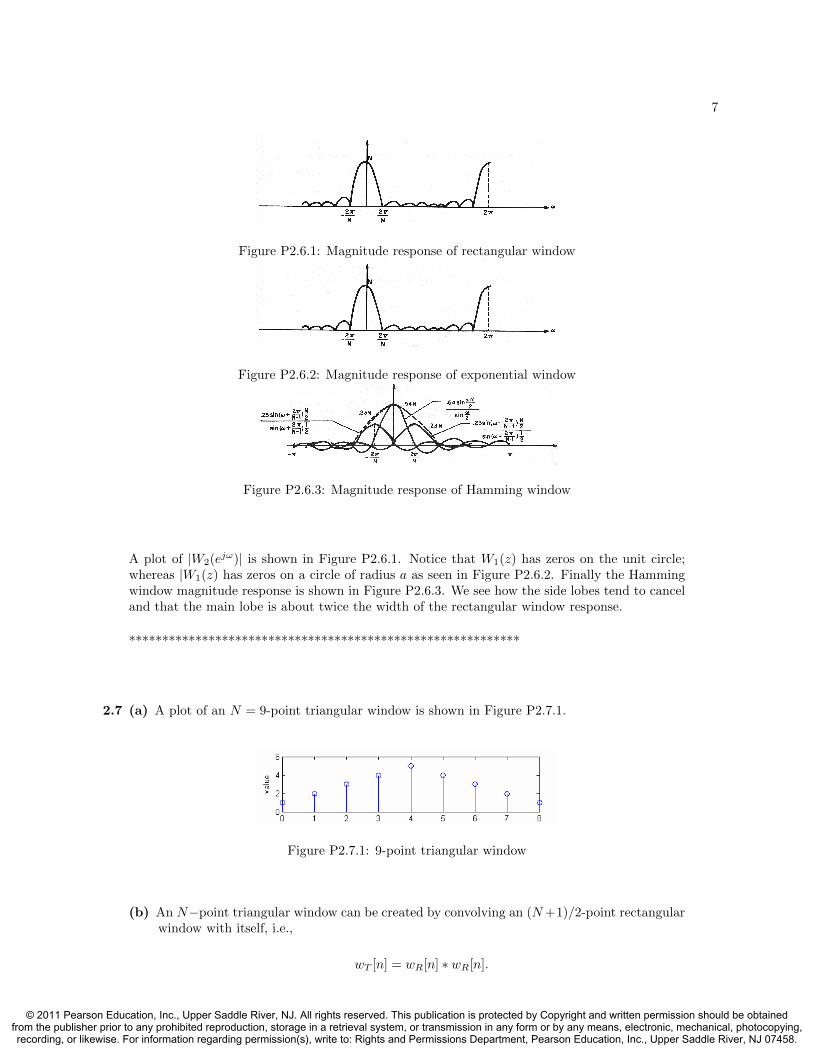
Figure P2.6.1: Magnitude response of rectangular window

Figure P2.6.2: Magnitude response of exponential window

Figure P2.6.3: Magnitude response of Hamming window

A plot of |W2(ejω)| is shown in Figure P2.6.1. Notice that W1(z) has zeros on the unit circle;whereas |W1(z) has zeros on a circle of radius a as seen in Figure P2.6.2. Finally the Hammingwindow magnitude response is shown in Figure P2.6.3. We see how the side lobes tend to canceland that the main lobe is about twice the width of the rectangular window response.

***********************************************************

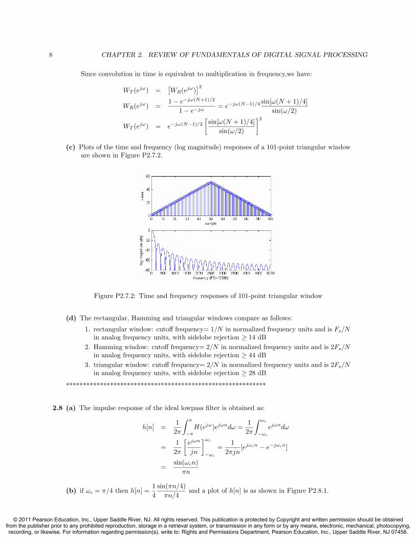
2.7 (a) A plot of an N = 9-point triangular window is shown in Figure P2.7.1.

Figure P2.7.1: 9-point triangular window

(b) An N−point triangular window can be created by convolving an (N+1)/2-point rectangularwindow with itself, i.e.,

wT [n] = wR[n] ∗ wR[n].



Since convolution in time is equivalent to multiplication in frequency,we have:

WT (ejω) =[WR(ejω)

]2WR(ejω) =

1− e−jω(N+1)/2

1− e−jω= e−jω(N−1)/4 sin[ω(N + 1)/4]

sin(ω/2)

WT (ejω) = e−jω(N−1)/2

[sin[ω(N + 1)/4]

sin(ω/2)

]2

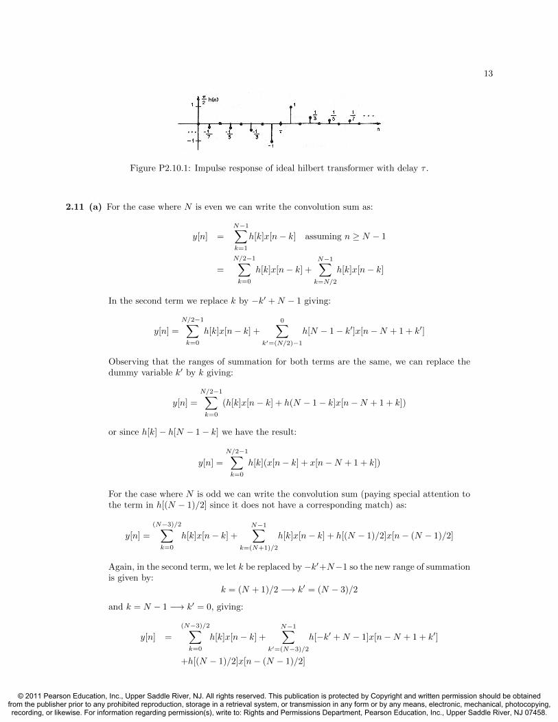
(c) Plots of the time and frequency (log magnitude) responses of a 101-point triangular windoware shown in Figure P2.7.2.

Figure P2.7.2: Time and frequency responses of 101-point triangular window

(d) The rectangular, Hamming and triangular windows compare as follows:

1. rectangular window: cutoff frequency= 1/N in normalized frequency units and is Fs/Nin analog frequency units, with sidelobe rejection ≥ 14 dB

2. Hamming window: cutoff frequency= 2/N in normalized frequency units and is 2Fs/Nin analog frequency units, with sidelobe rejection ≥ 44 dB

3. triangular window: cutoff frequency= 2/N in normalized frequency units and is 2Fs/Nin analog frequency units, with sidelobe rejection ≥ 28 dB

***********************************************************

2.8 (a) The impulse response of the ideal lowpass filter is obtained as:

h[n] =1

2π

∫ π

−πH(ejω)ejωndω =

1

2π

∫ ωc

−ωcejωndω

=1

2π

[ejωn

jn

]ωc−ωc

=1

2πjn[ejωcn − e−jωcn]

=sin(ωcn)

πn

(b) if ωc = π/4 then h[n] =1

4

sin(πn/4)

πn/4and a plot of h[n] is as shown in Figure P2.8.1.


9

Figure P2.8.1: Impulse response of ideal lowpass filter.

Figure P2.8.2: Parallel combination of ideal filters.

(c) One apporach to obtaining the desired impulse response is to view H(ejω) as a parallelcombination of lowpass, highpass, and zero phase filters, as shown in Figure P2.8.2.

We can express HHP (ejω) in terms of a lowpass filter with cutoff frequency π−ωb with thepassband shifted by π. From Part (a) we have:

HLP (ejω)←→ sin(ωan)

πn

where ωa is the cutoff, giving:

HHP (ejω) = HLP (ej(ω−π))←→ ejπnsin[(π − ωb)n]

πn

where π − ωb is the cutoff frequency.

The allpass has the property:

HAP (ejω) = 1←→ δ[n]

Putting it all together we get:

h[n] = δ[n]− sin(ωan)

πn− ejπn sin[(π − ωb)n]

πn

= δ[n]− sin(ωan)

πn− (−1)n

sin[(π − ωb)n]

πn



(d) When ωa = π/4 and ωb = 3π/4, we can express h[n] for the bandpass filter as:

h[n] = δ[n]− 0.25 sin(πn/4)

πn/4− (−1)n

sin[(π − 3π/4)n]

πn

= δ[n]− 0.25 sin(πn/4)

πn/4− (−1)n

0.25 sin(πn/4)

πn/4

= δ[n]− 0.25 sin(πn/4)

πn/4[1 + (−1)n]

A plot of h[n] for the bandpass filter is shown in Figure P2.8.3.

Figure P2.8.3: Impulse response of ideal bandpass filter.

***********************************************************

2.9 (a) The magnitude response of an ideal differentiator is:

|H(ejω)| = |ω|

and the phase response is:

argH(ejω) =

−ωτ + π/2 ω > 0

−ωτ − π/2 ω < 0

A plot of the magnitude and phase is given in Figure P2.9.1.

Figure P2.9.1: Magnitude and phase responses of ideal differentiator.


11

(b) The impulse response of the ideal differentiator is:

h[n] =1

2π

∫ π

−πH(ejω)ejωndω =

j

2π

∫ π

−πωejω(n−τ)dω

=j

2π

[ejω(n−τ)

(j(n− τ))2[jω(n− τ)− 1]

]π−π

=−j

2π(n− τ)2

[ejπ(n−τ)(jπ(n− τ)− 1)− e−jπ(n−τ)(−jπ(n− τ)− 1)

]=

−j2π(n− τ)2

[jπ(n− τ)[ejπ(n−τ) + e−jπ(n−τ)] + e−jπ(n−τ) − ejπ(n−τ)

]=

cos[π(n− τ)]

(n− τ)− sin[(π)n− τ)]

π(n− τ)2

(c) Using τ = (N − 1)/2 with N odd, we get:

h[n] =cos[(π/2)(2n−N + 1)]

n− (N − 1)/2− sin[(π/2)(2n−N + 1)]

π(n− (N − 1)/2))2

Note that 2n is always even, and for n odd, −N + 1 is even, therefore:

sin[(π/2)(2n−N + 1)] = 0, n 6= (N − 1)/2

and

h[n] =cos[(π/2)(2n−N + 1)]

n− (N − 1)/2)=

(−1)n+1

n− (N − 1)/2)n 6= (N − 1)/2

We see that h[n] tends to decrease as 1/n. Thus for N = 11 and τ = 5 we get:

h[n] =

(−1)n+1

n− 5n 6= 5

0 n = 5

A plot of h[n] for an ideal differentiator with N = 11 is shown in Figure P2.9.2.

Figure P2.9.2: Impulse response of ideal N = 11 differentiator.

Note that the value of h[n] for n = 5 is obtained from the equation:

h[n]|n=5 =

[1

2π

∫ π

−πjωejω(n−5)dω

]n=5

=j

2π

∫ π

−πωdω = 0

(d) When τ = (N − 1)/2 and N is even, then cos[(π/2)(2n−N + 1)] = 0 and we get:

h[n] =sin[(π/2)(2n−N + 1)]

π [n− (N − 1)/2]2 =

(−1)n

π[n− (N − 1)/2)]2



Figure P2.9.3: Impulse response of ideal N = 10 differentiator.

For N = 10, τ = 9/2 and h[n] =(−1)n

π(n− 9/2)2. A plot of h[n] for an N = 10 point ideal

differentiator is given in Figure P2.9.3.

***********************************************************

2.10 The term e−jωτ corresponds to a shift of τ samples in the impulse response. Therefore, start bydefining the frequency response without delay as:

H ′(ejω) =

−j 0 < ω < π

j −π < ω < 0

We solve for h′[n] as:

h′[n] =1

2π

∫ 0

−πjejωndω −

∫ π

0

jejωndω

=

1

2π

ejωn

n

∣∣∣∣0−π− ejωn

n

∣∣∣∣π0

=−1

2πn

ejπn + e−jπn − 2

=

1

πn[1− cos(πn)], n 6= 0

where we note that at n = 0 we get h′[n] = 0.

Inserting the appropriate shift of τ samples, we obtain:

h[n] = h′[n− τ ] =1

π(n− τ)[1− cos[π(n− τ)]], n 6= 0

Using the trigonometric identity (1/2)− (1/2) cos(2θ) = sin2(θ) we can rewrite h[n] as:

h[n] =

2 sin2(

π(n− τ)

2)

π(n− τ), n 6= τ

0 n = τ

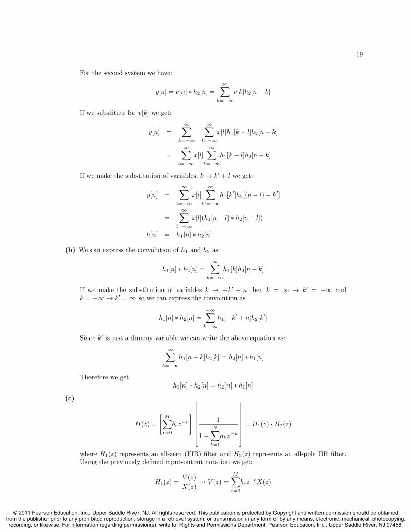
which is plotted in Figure P2.10.1.

***********************************************************


13

Figure P2.10.1: Impulse response of ideal hilbert transformer with delay τ .

2.11 (a) For the case where N is even we can write the convolution sum as:

y[n] =N−1∑k=1

h[k]x[n− k] assuming n ≥ N − 1

=

N/2−1∑k=0

h[k]x[n− k] +N−1∑k=N/2

h[k]x[n− k]

In the second term we replace k by −k′ +N − 1 giving:

y[n] =

N/2−1∑k=0

h[k]x[n− k] +

0∑k′=(N/2)−1

h[N − 1− k′]x[n−N + 1 + k′]

Observing that the ranges of summation for both terms are the same, we can replace thedummy variable k′ by k giving:

y[n] =

N/2−1∑k=0

(h[k]x[n− k] + h(N − 1− k]x[n−N + 1 + k])

or since h[k]− h[N − 1− k] we have the result:

y[n] =

N/2−1∑k=0

h[k](x[n− k] + x[n−N + 1 + k])

For the case where N is odd we can write the convolution sum (paying special attention tothe term in h[(N − 1)/2] since it does not have a corresponding match) as:

y[n] =

(N−3)/2∑k=0

h[k]x[n− k] +

N−1∑k=(N+1)/2

h[k]x[n− k] + h[(N − 1)/2]x[n− (N − 1)/2]

Again, in the second term, we let k be replaced by −k′+N−1 so the new range of summationis given by:

k = (N + 1)/2 −→ k′ = (N − 3)/2

and k = N − 1 −→ k′ = 0, giving:

y[n] =

(N−3)/2∑k=0

h[k]x[n− k] +N−1∑

k′=(N−3)/2

h[−k′ +N − 1]x[n−N + 1 + k′]

+h[(N − 1)/2]x[n− (N − 1)/2]



Figure P2.11.1: Implementation of N even FIR linear phase filter.

Figure P2.11.2: Implementation of N odd FIR linear phase filter.

or, equivalently:

y[n] =

(N−3)/2∑k=0

h[k](x[n− k] + x[n−N + 1 + k]) + h[(N − 1)/2]x[n− (N − 1)/2]

(b) For the case where N is even, we see that the first term in the expression for y[n] correspondsto a “normal” FIR filter with filter length of (N −2)/2. The second term is implemented bydelaying the samples by an amount of N/2 and then feeding these samples into the FIR filterfrom the opposite end. This is illustrated by the filter structure shown in FigureP2.11.1.

For the case where N is odd, a slight modification is required to account for the unmatchedsample in the impulse response. The appropriate direct-form realization is given in Fig-ure P2.11.2.

***********************************************************

2.12 (a) We can take the z-transform of the difference equation, giving:

Y (z) =X(z)− 1

4X(z)z−1

1− 1

3z−1

H(z) =Y (z)

X(z)=

1− 1

4z−1

1− 1

3z−1

, |z| > 1/3

(b) The z-transform of H(z) shows that there is a zero at z = 1/4 and a pole at z = 1/3

(c) With input x[n] = u[n], we solve for X(z) and then use a partial fraction expansion to solvefor Y (z) and then y[n], as:


15

X(z) =1

1− z−1

Y (z) =1− 1

4z−1

(1− z−1)(1− 1

3z−1)

=A

1− z−1+

B

1− 1

3z−1

We can now solve for A,B by matching terms, giving:

A+B = 1, ⇒ B = 1−A

−1

3A−B = −1

4

−1

3A− 1 +A = −1

4A = 9/8, B = −1/8

We now solve for Y (z) and y[n] as:

Y (z) =9/8

1− z−1− 1/8

1− 1

3z−1

y[n] = (9/8)u[n]− (1/8)

(1

3

)nu[n]

(d) We solve for Hi(z) as the inverse of H(z) giving:

Hi(z) =1

H(z)=

1− 1

3z−1

1− 1

4z−1

=1

1− 1

4z−1

−

1

3z−1

1− 1

4z−1

|z| > 1/4 stable inverse filter

hi[n] =

(1

4

)nu[n]−

(1

3

)(1

4

)n−1

u[n− 1]

***********************************************************

2.13 (a) We can solve for H(z) as:

Y (z) = αz−1Y (z) +X(z)

Y (z)(1− αz−1) = X(z)

H(z) =Y (z)

X(z)=

1

(1− αz−1)



(b) Since the difference equation indicates that h[n] is a causal (right-sided) sequence, the ap-propriate inverse z−transform is:

h[n] = αnu[n]

(c) BIBO stability requires |α| < 1.

(d) For the condition that h[n] = αnu[n] < e−1 for nT < 2 msec we first solve for n insamples as:

n =2x10−1

T=

0.002

T

We can now solve for α as:

(α)(0.002/T ) = e−1

lnα =−T

2x10−3

α = exp[−500T ]

***********************************************************

2.14 (a) A complex zero occurs at z = e±jθ and a complex pole occurs at z = re±jθ. The plotof the complex pole-zero locations for r = 0.95 and θ = 60o (π/3) radians is shown inFigure P2.14.1.

Figure P2.14.1: Pole-Zero Plot for Notch Filter.

(b) The log magnitude plot is shown in Figure P2.14.2.

(c) The maximum value of |H(ejω)| occurs at either ω = 0 or ω = π, depending on the value ofθ. The maximum value ≈ 1 (i.e., 0 dB) if r is close to 1.0.

(d) For a notch to occur at 60 Hz, for a sampling rate of fS = 8000 Hz, we need a value ofθ = 60 ∗ 2π/8000 = 3π/200 radians.

***********************************************************


17

Figure P2.14.2: Log Magnitude Response for Notch Filter.

2.15 (a) We solve for H(ejω) as:

H(ejω) =∞∑

n=−∞h[n]e−jωn

=∞∑n=0

(1

2

)ncos(πn

2

)e−jωn

=∞∑n=0

(1

2

)n [ejπn/2 + e−jπn/2

2

]e−jωn

=1

2

∞∑n=0

[1

2ej(π/2−ω)

]n+

1

2

∞∑n=0

[1

2ej(−π/2−ω)

]n=

(1/2)

1− (1/2)ej(π/2−ω)+

(1/2)

1− (1/2)ej(−π/2−ω)

=(1/2)

1− (1/2)je−jω+

(1/2)

1 + (1/2)je−jω

=1

1 + (1/4)e−2jω

(b) The input can be written as a sum of eigenfunctions of the system, i.e.,

cos(πn

2

)=ejπn/2 + e−jπn/2

2

The system response to an eigenfunction ejω1n is:

y[n] = H(ejω)|ω=ω1· ejω1n

Thus, from part (a), we get:

y[n] =

(1

2

)H(ejω)|ω=π/2 · ejπn/2 +

(1

2

)H(ejω)|ω=−π/2 · e−jπn/2

=

(1

2

)1

1 + (1/4)e−jπejπn/2 +

(1

2

)1

1 + (1/4)ejπe−jπn/2

=

(4

3

)cos(πn/2)



***********************************************************

2.16 (a) The system function is of the form:

H(z) =

AM∏r=1

(1− crz−1)

N∏k=1

(1− dkz−1)

, A = gain constant

If M < N , we can consider this product form for H(z) to be the result of establishing acommon denominator for H(z) given by:

H(z) =N∑k=1

Ak(1− dkz−1)

The Ak’s are termed residues and should not be confused with the gain constant, denotedin this problem by A. Since, in the product form, the numerator is a polynomial in z−1,and since M < N , we are assured that the Ak’s are just complex constants.

In order to determine a particular Am, we multiply both sides of the expression for H(z)by the corresponding denominator term so that

(1− dmz−1)H(z) =N∑k=1

k 6=m

(1− dmz−1)Ak(1− dkz−1)

= Am

If we let z−1 −→ dm, then on the right hand side all the terms multiplied by (1 − dmz−1)will vanish leaving only Am. On the left-hand side, the term (1− dmz−1) in the numeratorcancels with the denominator term. The final result is:

A

M∏r=1

(1− crd−1m )

(1− dkd−1m )

= Am, m = 1, 2, ..., N

In this manner, all the Ak’s are determined.

(b) Given hk[n] = Ak(dk)nu[n] we can compute the z−transform as:

H(z) =∞∑

n=−∞hk[n]z−n =

∞∑n=0

Ak(dk)nz−n

= Ak

∞∑n=0

(dkz−1)n

=Ak

1− dkz−1, |dkz−1| < 1 or |z| > dk

***********************************************************

2.17 (a) For the first system we have:

v[n] = x[n] ∗ h1[n] =∞∑

l=−∞

x[l]h1[n− l]


19

For the second system we have:

y[n] = v[n] ∗ h2[n] =∞∑

k=−∞

v[k]h2[n− k]

If we substitute for v[k] we get:

y[n] =∞∑

k=−∞

∞∑l=−∞

x[l]h1[k − l]h2[n− k]

=∞∑

l=−∞

x[l]∞∑

k=−∞

h1[k − l]h2[n− k]

If we make the substitution of variables, k → k′ + l we get:

y[n] =∞∑

l=−∞

x[l]∞∑

k′=−∞

h1[k′]h2[(n− l)− k′]

=

∞∑l=−∞

x[l](h1[n− l] ∗ h2[n− l])

h[n] = h1[n] ∗ h2[n]

(b) We can express the convolution of h1 and h2 as:

h1[n] ∗ h2[n] =∞∑

k=−∞

h1[k]h2[n− k]

If we make the substitution of variables k → −k′ + n then k = ∞ → k′ = −∞ andk = −∞→ k′ =∞ so we can express the convolution as

h1[n] ∗ h2[n] =−∞∑k′=∞

h1[−k′ + n]h2[k′]

Since k′ is just a dummy variable we can write the above equation as:

∞∑k=−∞

h1[n− k]h2[k] = h2[n] ∗ h1[n]

Therefore we get:h1[n] ∗ h2[n] = h2[n] ∗ h1[n]

(c)

H(z) =

[M∑r=0

brz−r

]1

1−N∑k=1

akz−k

= H1(z) ·H2(z)

where H1(z) represents an all-zero (FIR) filter and H2(z) represents an all-pole IIR filter.Using the previously defined input-output notation we get:

H1(z) =V (z)

X(z)→ V (z) =

M∑r=0

brz−rX(z)



H2(z) =Y (z)

V (z)→ Y (z) = V (z) +

N∑k=1

akz−kY (z)

and we obtain the difference equations by inverse transforming these relations, giving:

v[n] =M∑r=0

brx[n− r]

y[n] = v[n]−N∑k=1

aky[n− k]

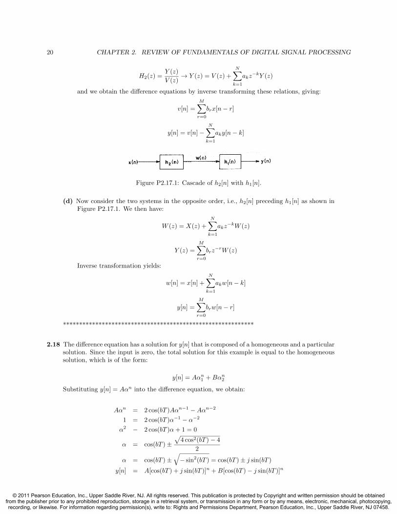
Figure P2.17.1: Cascade of h2[n] with h1[n].

(d) Now consider the two systems in the opposite order, i.e., h2[n] preceding h1[n] as shown inFigure P2.17.1. We then have:

W (z) = X(z) +N∑k=1

akz−kW (z)

Y (z) =

M∑r=0

brz−rW (z)

Inverse transformation yields:

w[n] = x[n] +

N∑k=1

akw[n− k]

y[n] =M∑r=0

brw[n− r]

***********************************************************

2.18 The difference equation has a solution for y[n] that is composed of a homogeneous and a particularsolution. Since the input is zero, the total solution for this example is equal to the homogeneoussolution, which is of the form:

y[n] = Aαn1 +Bαn2

Substituting y[n] = Aαn into the difference equation, we obtain:

Aαn = 2 cos(bT )Aαn−1 −Aαn−2

1 = 2 cos(bT )α−1 − α−2

α2 − 2 cos(bT )α+ 1 = 0

α = cos(bT )±√

4 cos2(bT )− 4

2

α = cos(bT )±√− sin2(bT ) = cos(bT )± j sin(bT )

y[n] = A[cos(bT ) + j sin(bT )]n +B[cos(bT )− j sin(bT )]n


21

The initial conditions will determine the appropriate values for A and B. Alternately, we canchoose A and B and then determine the corresponding initial conditions. First we rewrite y[n]using Euler’s identity as:

y[n] = AejbTn +Be−jbTn

(a) y[n] = cos(bTn)u[n]⇒ A = B = 1/2 with initial conditions:

y[−1] = Ae−jbT +BejbT =1

2[e−jbT + ejbT ]

y[−1] = cos(bT )

y[−2] =1

2[e−j2bT + ej2bT ] = cos(2bT )

y[n] = cos(bTn)u[n]

(b) Similarly y[n] = sin(bTn)u[n] ⇒ A = −B =1

2jso we require that y[−1] =

1

2j[e−jbT −

ejbT ] = − sin(bT ) and similarly y[−2] = − sin(2bT ).

***********************************************************

2.19 (a) The network diagram for this system is shown in Figure P2.19.1.

Figure P2.19.1: Network diagram of set of difference equations.

(b) Using transforms we get:

Y1(z) = Az−1Y1(z) +Bz−1Y2(z) +X(z)

Y2(z) = Cz−1Y1(z) +Dz−1Y2(z)

Solving the second equation for Y2(z) gives:

Y2(z) =Cz−1Y1(z)

1−Dz−1

We now substitute in the first equation giving:

Y1(z) = Az−1Y1(z) +Bz−1

[Cz−1Y1(z)

1−Dz−1

]+X(z)

=X(z)

1−Az−1 − BCz−2

1−Dz−1

Y1(z)

X(z)= H1(z) =

1−Dz−1

1− (A+D)z−1 + (AD −BC)z−2



From the second equation we get:

H2(z) =Y2(z)

X(z)=

Cz−1

(1−Dz−1)

Y1(z)

X(z)=

Cz−1

1− (A+D)z−1 + (AD −BC)z−2

(c) If A = D = r cos(θ) and C = −B = r sin(θ) we get:

H1(z) =1− r cos(θ)z−1

1− 2r cos(θ)z−1 + r2z−2

=A1

1− r(cos(θ) + j sin(θ))z−1+

A∗11− r(cos(θ)− j sin(θ))z−1

where:

A1 = limz→r(cos(θ)+j sin(θ))

[z − r cos(θ)

z − r(cos(θ)− j sin(θ))

]=

jr sin(θ)

2jr sin(θ)=

1

2

H1(z) =1/2

1− r(cos(θ) + j sin(θ))z−1+

1/2

1− r(cos(θ)− j sin(θ))z−1

We assume the region of convergence for H1(z) includes the unit circle. Inverse transforminggives:

h1[n] =1

2[r cos(θ) + j sin(θ))]nu[n] +

1

2[r cos(θ)− j sin(θ))]nu[n] for |r| < 1

=1

2[rejθ]nu[n]− 1

2[re−jθ]nu[n]

=1

2rn[ejθn + e−jθn]u[n] = rn cos(θn)u[n]

= rn cos(θn)u[n]

H2(z) =A1

1− r cos(θ) + j sin(θ))z−1+

A∗11− r cos(θ)− j sin(θ))z−1

where:

A1 = limz→r(cos(θ)+j sin(θ))

[r sin(θ)

z − r(cos(θ)− j sin(θ))

]=

r sin(θ)

2jr sin(θ)=

1

2j

H2(z) =1/(2j)

1− r(cos(θ) + j sin(θ))z−1− 1/(2j)

1− r(cos(θ)− j sin(θ))z−1

h2[n] = rn sin(θn)u[n]

***********************************************************

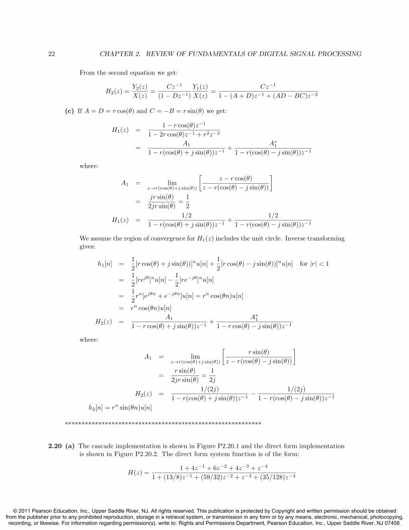
2.20 (a) The cascade implementation is shown in Figure P2.20.1 and the direct form implementationis shown in Figure P2.20.2. The direct form system function is of the form:

H(z) =1 + 4z−1 + 6z−2 + 4z−3 + z−4

1 + (13/8)z−1 + (59/32)z−2 + z−3 + (35/128)z−4


23

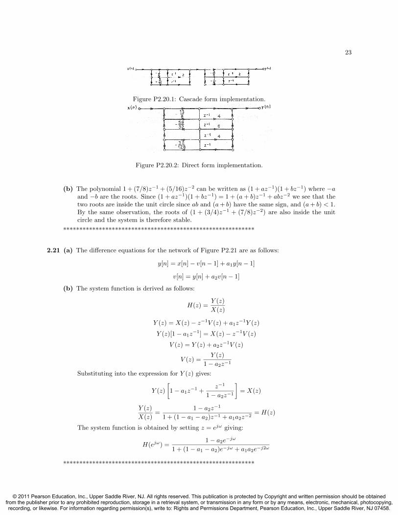
Figure P2.20.1: Cascade form implementation.

Figure P2.20.2: Direct form implementation.

(b) The polynomial 1 + (7/8)z−1 + (5/16)z−2 can be written as (1 + az−1)(1 + bz−1) where −aand −b are the roots. Since (1 + az−1)(1 + bz−1) = 1 + (a+ b)z−1 + abz−2 we see that thetwo roots are inside the unit circle since ab and (a+ b) have the same sign, and (a+ b) < 1.By the same observation, the roots of (1 + (3/4)z−1 + (7/8)z−2) are also inside the unitcircle and the system is therefore stable.

***********************************************************

2.21 (a) The difference equations for the network of Figure P2.21 are as follows:

y[n] = x[n]− v[n− 1] + a1y[n− 1]

v[n] = y[n] + a2v[n− 1]

(b) The system function is derived as follows:

H(z) =Y (z)

X(z)

Y (z) = X(z)− z−1V (z) + a1z−1Y (z)

Y (z)[1− a1z−1] = X(z)− z−1V (z)

V (z) = Y (z) + a2z−1V (z)

V (z) =Y (z)

1− a2z−1

Substituting into the expression for Y (z) gives:

Y (z)

[1− a1z

−1 +z−1

1− a2z−1

]= X(z)

Y (z)

X(z)=

1− a2z−1

1 + (1− a1 − a2)z−1 + a1a2z−2= H(z)

The system function is obtained by setting z = ejω giving:

H(ejω) =1− a2e

−jω

1 + (1− a1 − a2)e−jω + a1a2e−j2ω

***********************************************************



2.22 For Network #1 we have:

H1(z) =1

1− b1z−1− 1

1− b2z−1=

(b1 − b2)z−1

1− (b1 + b2)z−1 + b1b2z−2

For Network #2 we have:

H2(z) =

[1

1− a1z−1

] [z−1

1− a2z−1

]a3

H2(z) =a3z−1

1− (a1 + a2)z−1 + a1a2z−2

We require that a3 = (b1 − b2), (a1 + a2) = (b1 + b2) and a1a2 = b1b2 which implies that eithera1 = b1 and a2 = b2 or else a1 = b2 and a2 = b1.

***********************************************************

2.23 (a) We can factor the H(z) polynomial and find the root locations from the factored form. Theresult of factoring is:

H(z) =1− 2e−aT cos(bT ) + e−2aT

1− 2e−aT cos(bT )z−1 + e−2aT z−2

H(z) =z2(1− 2e−aT cos(bT ) + e−2aT )

(z − e−(a+jb)T )(z − e−(a−jb)T )

The roots of H(z) are plotted in Figure P2.23.1.

Figure P2.23.1: Location of poles and zeros of H(z) in the Z−plane.

Figure P2.23.2: Frequency response of the resonator.


25

(b) We can invert H(z) using a partial fraction expansion giving the impulse response:

h[n] =

(1− e−aT cos(bT ) + e−2aT )

sin(bT )e−aTn sin[(n+ 1)bT ] n ≥ 0

0 n < 0

(c) A plot of the frequency response of the resonator is given in Figure P2.23.2.

***********************************************************

2.24 (a) The z−transform and Fourier transform are:

X(z) =∞∑

n=−∞x[n]z−n = 1 + 0.5z−5

X(ejω) = 1 + 0.5e−j5ω

(b) The N -point DFT is obtained by evaluating X(ejω) at N evenly spaced frequencies on theunit circle; i.e., at the set of values:

ω =2πk

N, k = 0, 1, . . . , N − 1

Hence for the cases of N = 50 and N = 10 we get:

N = 50 X(ej2πk/50) = 1 + 0.5e−jπk/5, k = 0, 1, . . . , 49

N = 10 X(ej2πk/10) = 1 + 0.5e−jπk, k = 0, 1, . . . , 9

For N = 5 the DFT is not properly defined since x[n] is a 6-point sequence. Thus we caneither use the first five values of x[n], giving:

X(ej2πk/5) = 1, k = 0, 1, . . . , 4

or we can wrap x[n] around a cylinder, i.e., take the result modulo 4, giving:

X(ej2πk/5) = 1.5, k = 0, 1, . . . , 4

(c) For N = 5 the DFT values can either be considered the same as the DFT for N = 50,evaluated every 10th point, or they can differ depending on the signal values used for thecomputation.

(d) The DFT X[k] is the Fourier transform evaluated at N equally spaced frequencies (pointsaround the unit circle) if N is greater than or equal to the duration of the sequence. Oth-erwise X[k] and X(ejω) need not be directly related. For N = 5 the DFT values can eitherbe considered the same as

***********************************************************

2.25 (a) The time duration, TD, of an L = 1024 sample sequence with a sampling rate of Fs = 1/T =20, 000 samples/second is:

TD =L

Fs=

1024

20, 000= 5115× 10−4 seconds = 51.15 msec



(b) The frequency resolution in radians, ∆ω, between the DFT values is:

∆ω =2π

NFFT=

2π

1024

where NFFT is the size of the DFT. Using the relationship between analog and digitalfrequency, we can determine the analog frequency resolution as:

ω = ΩT

∆Ω =∆ω

T=

2π

(1024)(5× 10−5)

∆f =∆Ω

2π=

1

(1024)(5× 10−5)= 19.531 Hz

(c) If we change the duration of the speech segment to 512 samples, the time duration wouldbecome half of the previous duration or 25.55 msec. Using a 1024-point DFT will producethe same frequency resolution of 19.531 Hz as previously since the frequency resolutiondepends only on the size of the FFT that is performed.

***********************************************************

2.26 Assume xmin[n] is a minimum-phase signal with all of its poles and zeros inside the unit circle.Using z-transforms we can express Xmin(z) as:

xmin[n]←→ Xmin(z) =

∞∑n=−∞

xmin[n] z−n =

Nz∏i=1

(1− ai z−i)

Np∏i=1

(1− bi z−i)

Since xmin[n] is a minimum-phase signal, then all the poles (z = bi) and zeros (z = ai) are insidethe unit circle. Therefore we have the constraint |ai| < 1 for all i and |bi| < 1 for all i. The signalxmax[n] = xmin[−n] has a z-transform of the form:

xmax[n]←→ Xmax(z) =∞∑

n=−∞xmax[n]z−n

=∞∑

n=−∞xmin[−n]z−n =

∞∑n=−∞

xmin[n](z−1)−n = Xmin(z−1)

=

Nz∏i=1

(1− aiz)

Np∏i=1

(1− biz)

Thus the signal xmin[−n] = xmax[n] has zeros at z = 1/ai > 1 and poles at z = 1/bi > 1. Thusall zeros and poles of xmin[−n] = xmax[n] are outside the unit circle, so xmin[−n] = xmax[n] is amaximum phase signal whenever xmin[n] is a minimum phase signal.

***********************************************************


27

2.27 We need to utilize the series expansion:

1

1− x= 1 + x+ x2 + x3 + . . . =

∞∑n=0

xn

or, equivalently,

1− x =1

1 + x+ x2 + x3 + . . .=

1∞∑n=0

xn

(a) Thus we can utilize the above equation to write the expression for a single zero as:

z − a = (1− az−1) z =z

1 + az−1 + a2z−2 + a3z−3 + . . .

=1

z−1(1 + az−1 + a2z−2 + a3z−3 + ...)

(b) When only a finite number of terms (poles) are used, the approximation to the real zerodepends on the location of the real zero. Thus, as |a| → 0, the approximation convergesmore rapidly.

(c) The first order approximation is:

z − a ≈ z

1 + az−1=

z2

z + a

i.e., a system with a real pole at z = −a. The second order approximation is:

z − a ≈ z

1 + az−1 + a2z−2=

z3

z2 + az + a2

i.e., a second order system with a complex pole at z = −a/2± j√

3a/2

(d) Similarly, we can represent a single pole as an infinite number of zeros using the expression:

1

z − b= z−1 + bz−2 + b2z−3 + . . .

***********************************************************

2.28 (a) The ideal solution to fractional delays is a multirate system. Thus for a delay of D = 1/2sample, the system would consist of an interpolator (by a factor of 2), a lowpass filter(with cutoff of half the original sampling frequency, a unit sample delay (at the interpolatedsampling rate), and a decimator (by a factor of 2) to restore the original sampling rate ofthe system. These operations are illustrated in Figure P2.28.1.

Figure P2.28.1: Ideal implementation of a delay of D = 1/2 sample.



(b) The simplest approximation to a D = 0.5 sample delay (without interpolation and decima-tion) is simple linear interpolation (i.e., average the neighboring samples with equal weight),giving values of α = 0.5 and β = 0.5.

In this case we get the resulting approximation to the ideal interpolator as:

y[n] = 0.5x[n] + 0.5x[n− 1]

H(z) = 0.5(1 + z−1)

H(ejω) = 0.5(1 + e−jω) = 0.5(1 + cos(ω)− j sin(ω))

|H(ejω)| = 0.5[(1 + cos(ω))2 + sin2(ω)]1/2

= [2 + 2 cos(ω)]1/2

=

√2

2(1 + cos(ω))1/2

By plotting |H(ejω)| versus ω we can see that the linear interpolator is basically a first orderapproximation to the ideal lowpass filter of the ideal interpolator which is flat in frequencyuntil the point ω = π/2 and then is zero from ω = π/2 to ω = π.

(c) If the delay is changed to D = 1/3 sample, the interpolator becomes a 3-to-1 interpolatorand the decimator becomes a 3-to-1 decimator, as shown in Figure P2.28.2.

Figure P2.28.2: Ideal implementation of a delay of D = 1/3 sample.

(d) The linear interpolation solution would just change the weights to reflect the desired delayof D = 1/3 sample, giving weights of α = 2/3 and β = 1/3.

(e) Since the desired delay is a rational fraction, the ideal solution becomes a multirate interpo-lator and a multirate decimator with a unit sample delay inserted in the middle. The signalprocessing operations (and the resulting sampling rates) are shown in Figure P2.28.3.

Figure P2.28.3: Ideal implementation of a delay of D = 3/10 sample using a single unit delay.

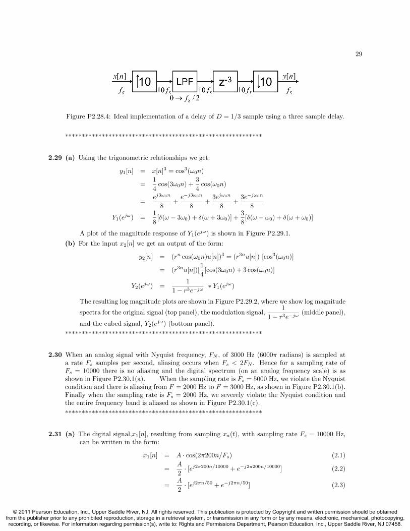
It is easily seen that the middle three blocks (the downsampling by a factor of 3-to-1 followedby unit sample delay followed by upsampling by a factor of 3-to-1) can be coalesed into asingle block with a delay of 3 samples at the higher sampling rate. Further the serialcombination of the remaining lowpass filters can be realized as a single lowpass filter, leadingto the ideal implementation shown in Figure P2.28.4.


29

Figure P2.28.4: Ideal implementation of a delay of D = 1/3 sample using a three sample delay.

***********************************************************

2.29 (a) Using the trigonometric relationships we get:

y1[n] = x[n]3 = cos3(ω0n)

=1

4cos(3ω0n) +

3

4cos(ω0n)

=ej3ω0n

8+e−j3ω0n

8+

3ejω0n

8+

3e−jω0n

8

Y1(ejω) =1

8[δ(ω − 3ω0) + δ(ω + 3ω0)] +

3

8[δ(ω − ω0) + δ(ω + ω0)]

A plot of the magnitude response of Y1(ejω) is shown in Figure P2.29.1.

(b) For the input x2[n] we get an output of the form:

y2[n] = (rn cos(ω0n)u[n])3 = (r3nu[n]) [cos3(ω0n)]

= (r3nu[n])[1

4[cos(3ω0n) + 3 cos(ω0n)]

Y2(ejω) =1

1− r3e−jω∗ Y1(ejω)

The resulting log magnitude plots are shown in Figure P2.29.2, where we show log magnitude

spectra for the original signal (top panel), the modulation signal,1

1− r3e−jω(middle panel),

and the cubed signal, Y2(ejω) (bottom panel).

***********************************************************

2.30 When an analog signal with Nyquist frequency, FN , of 3000 Hz (6000π radians) is sampled ata rate Fs samples per second, aliasing occurs when Fs < 2FN . Hence for a sampling rate ofFs = 10000 there is no aliasing and the digital spectrum (on an analog frequency scale) is asshown in Figure P2.30.1(a). When the sampling rate is Fs = 5000 Hz, we violate the Nyquistcondition and there is aliasing from F = 2000 Hz to F = 3000 Hz, as shown in Figure P2.30.1(b).Finally when the sampling rate is Fs = 2000 Hz, we severely violate the Nyquist condition andthe entire frequency band is aliased as shown in Figure P2.30.1(c).

***********************************************************

2.31 (a) The digital signal,x1[n], resulting from sampling xa(t), with sampling rate Fs = 10000 Hz,can be written in the form:

x1[n] = A · cos(2π200n/Fs) (2.1)

=A

2· [ej2π200n/10000 + e−j2π200n/10000] (2.2)

=A

2· [ej2πn/50 + e−j2πn/50] (2.3)



Figure P2.29.1: Magnitude spectrum of cubed cosine wave.

Figure P2.29.2: Log magnitude spectrum of modulated and cubed cosine wave.

which has a frequency response, X1(ejω), consisting of impulses at frequencies ±200 Hz. Asketch of the digital frequency response is shown in the top panel of Figure P2.31.1.

(b) In a similar manner, we can solve for the digital frequency response, X2(ejω), resulting fromsampling xb(t), with sampling rate Fs = 10000 Hz, resulting in:

x2[n] =B

2· [ej2π201n/Fs + e−j2π201n/Fs ] (2.4)

which has a frequency response X2(ejω), consisting of impulses at frequencies ±201 Hz. Asketch of the digital frequency response is shown in the bottom panel of Figure P2.31.1.

(c) A digital signal, x[n], is periodic with period P samples, if it obeys the relation:

x[n+ P ] = x[n] for all n and for P > 0 (2.5)

It is clear that x1[n] is periodic and of period P = 50 samples. It is somewhat more difficultto see that the signal x2[n] is also periodic but of period P = 10000 samples since the cosine


31

Figure P2.30.1: Digital spectra with different sampling rates.

Figure P2.31.1: Frequency responses of the two signals.

function satisfies the relationship:

cos(a+ b) = cos(a) cos(b)− sin(a) sin(b) (2.6)

x2[n+ 10000] = cos(2π201(n+ 10000)/10000) (2.7)

= cos(2π201n/10000) cos(2π201) (2.8)

− sin(2π201n/10000) sin(2π201) (2.9)

= cos(2π201n/10000) = x2[n] (2.10)

since cos(2π201) = 1 and sin(2π201) = 0 in the above equation.

***********************************************************


solution guide for theory and applications of digital speech processing · speech processing by...

Documents