speech coding: techniques, standards and applications · it involves the study of the techniques we...

Speech coding:

Analog and Telecommunication Electronics

Mini Project

Master Degree in Electronic Engineering

Professor: Dante Del CorsoStudent: Nadia Perreca, ID: 211012

Academic Year 2013-2014

Speech coding:

techniques, standards and applications

Introduction

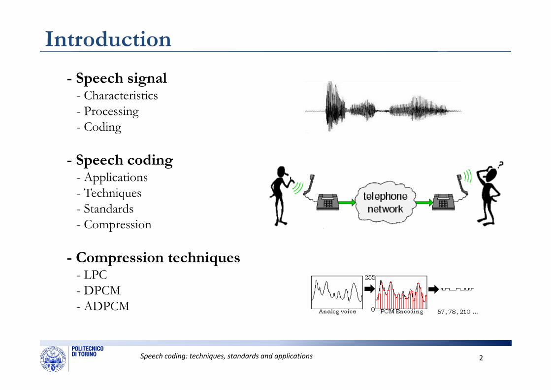
- Speech signal- Characteristics- Processing- Coding

- Speech coding- Applications- Techniques

Speech coding: techniques, standards and applications 2

- Techniques- Standards- Compression

- Compression techniques- LPC- DPCM- ADPCM

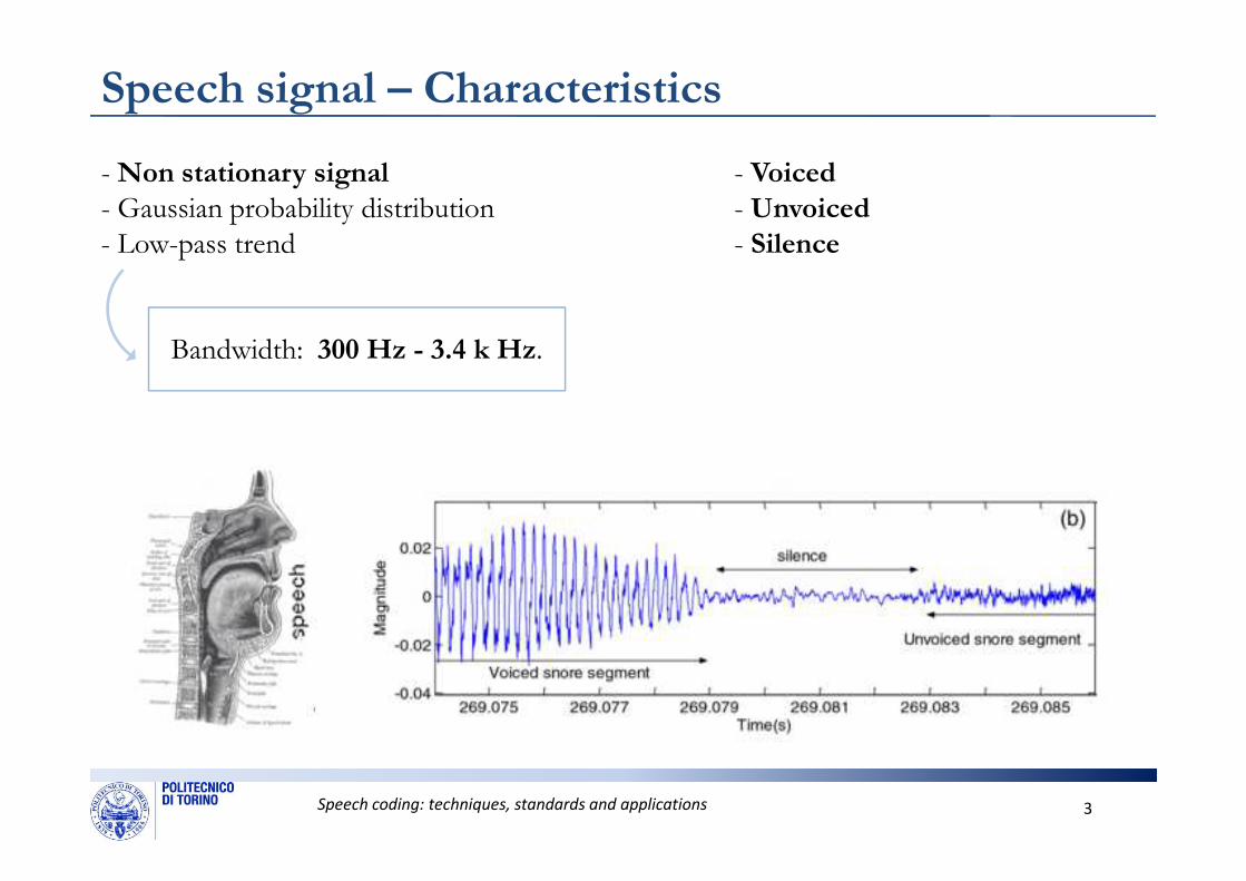
- Voiced

- Unvoiced

- Silence

- Non stationary signal

- Gaussian probability distribution- Low-pass trend

Bandwidth: 300 Hz - 3.4 k Hz.

Speech signal – Characteristics


Speech signals – Real speech signals

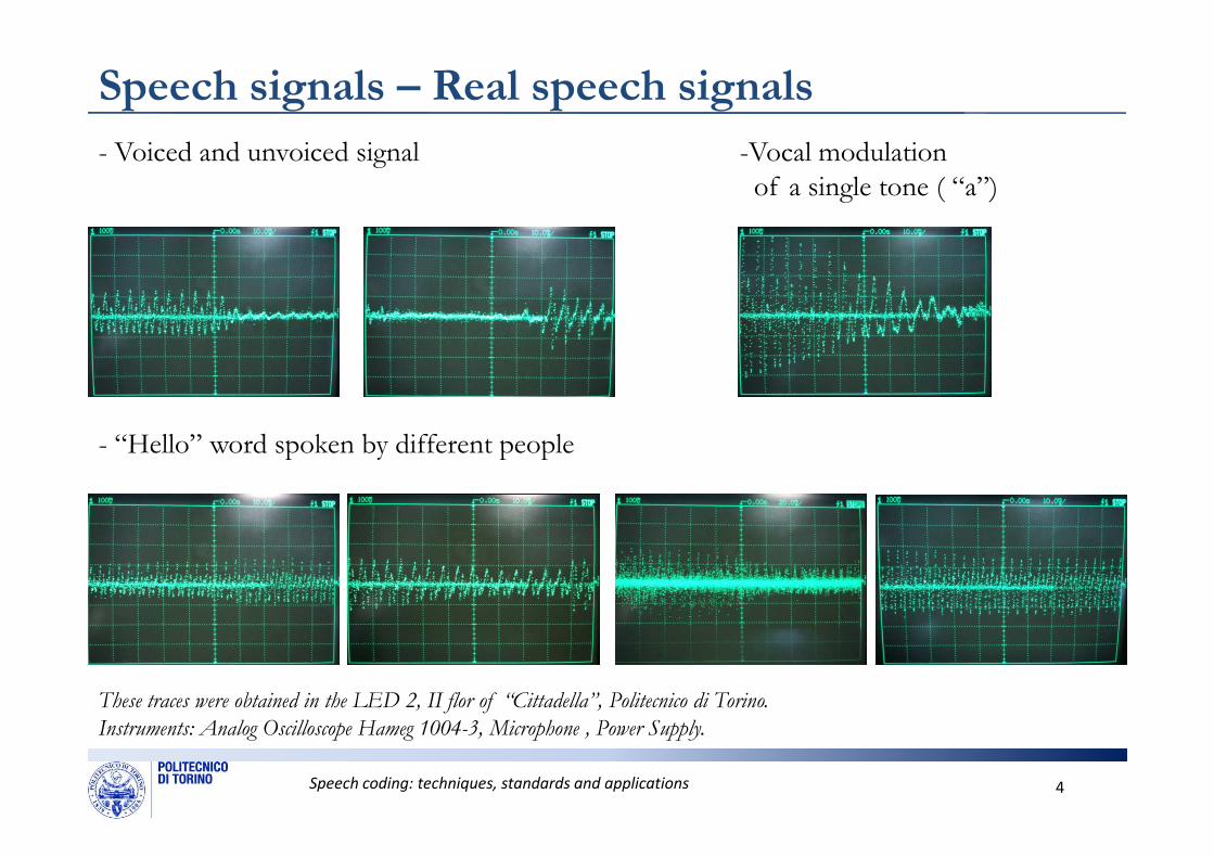
- Voiced and unvoiced signal -Vocal modulationof a single tone ( “a”)

- “Hello” word spoken by different people


- “Hello” word spoken by different people

These traces were obtained in the LED 2, II flor of “Cittadella”, Politecnico di Torino.

Instruments: Analog Oscilloscope Hameg 1004-3, Microphone , Power Supply.

Speech signal – How can we analyze them?

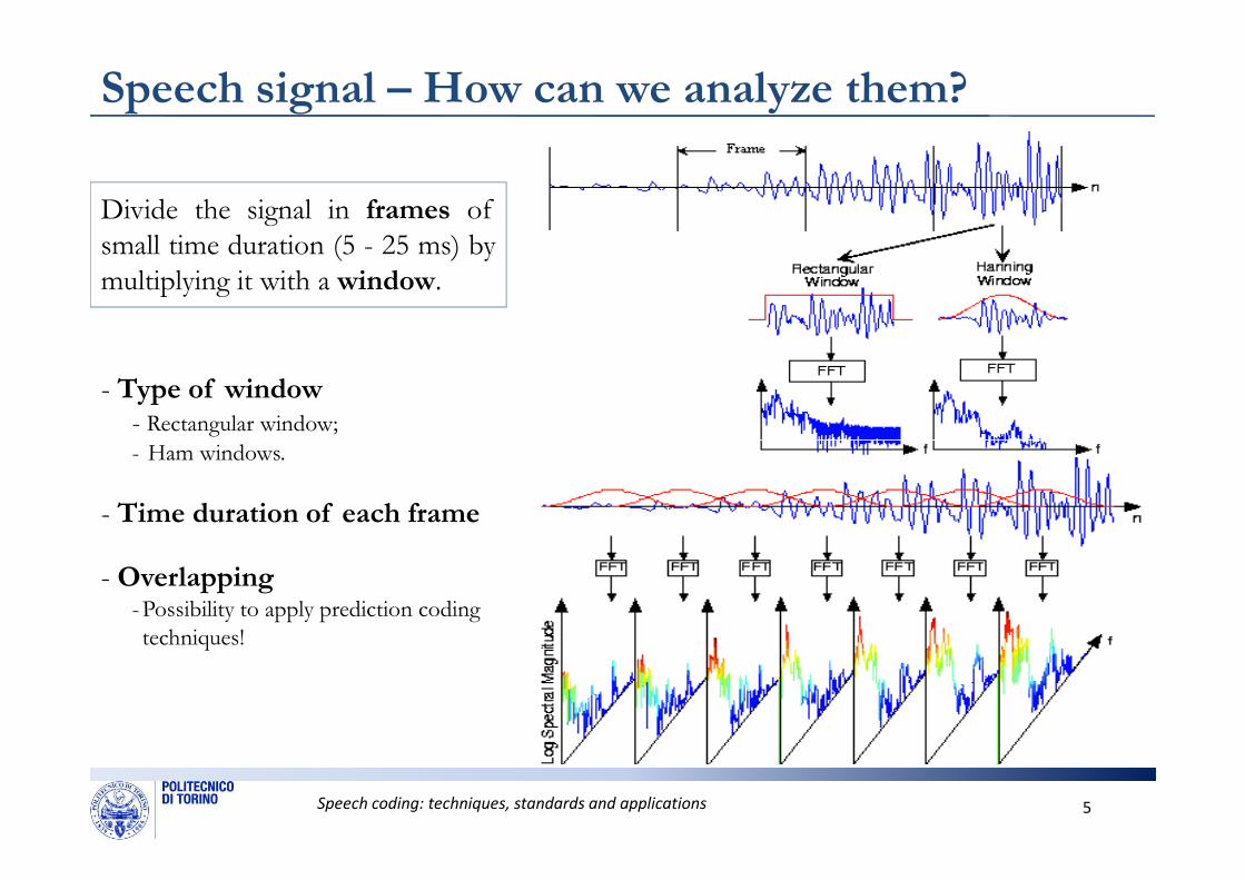
- Type of window- Rectangular window;- Ham windows.

Divide the signal in frames ofsmall time duration (5 - 25 ms) bymultiplying it with a window.


- Ham windows.

- Time duration of each frame

- Overlapping-Possibility to apply prediction coding

techniques!

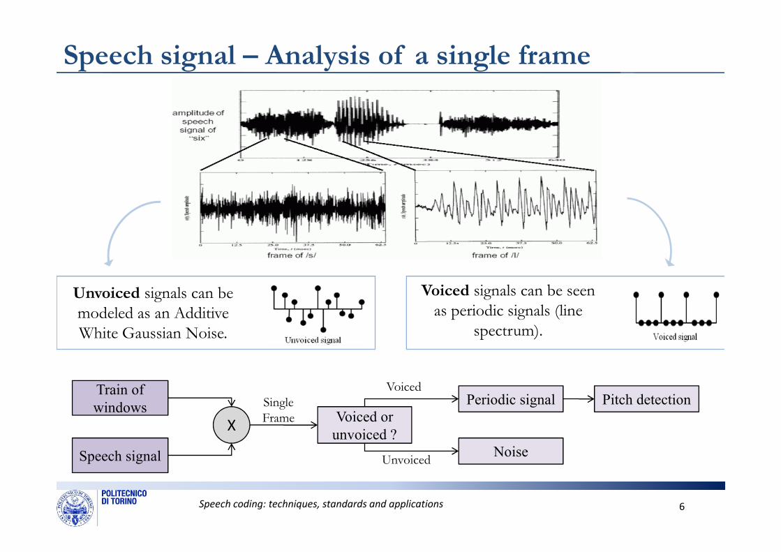
Speech signal – Analysis of a single frame


Voiced signals can be seen

as periodic signals (line

spectrum).

Unvoiced signals can be

modeled as an Additive

White Gaussian Noise.

Speech signal

Periodic signal

Voiced or

unvoiced ? X

Train of

windows

Noise

Voiced

Unvoiced

SingleFrame

Pitch detection

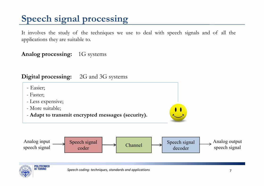
Speech signal processing

It involves the study of the techniques we use to deal with speech signals and of all the

applications they are suitable to.

Analog processing: 1G systems

Digital processing: 2G and 3G systems

- Easier;- Faster;


- Faster;

- Less expensive;

- More suitable;

- Adapt to transmit encrypted messages (security).

Speech signal

coderChannel

Speech signal

decoder

Analog output

speech signalSpeech signal

coder

Analog input

speech signal

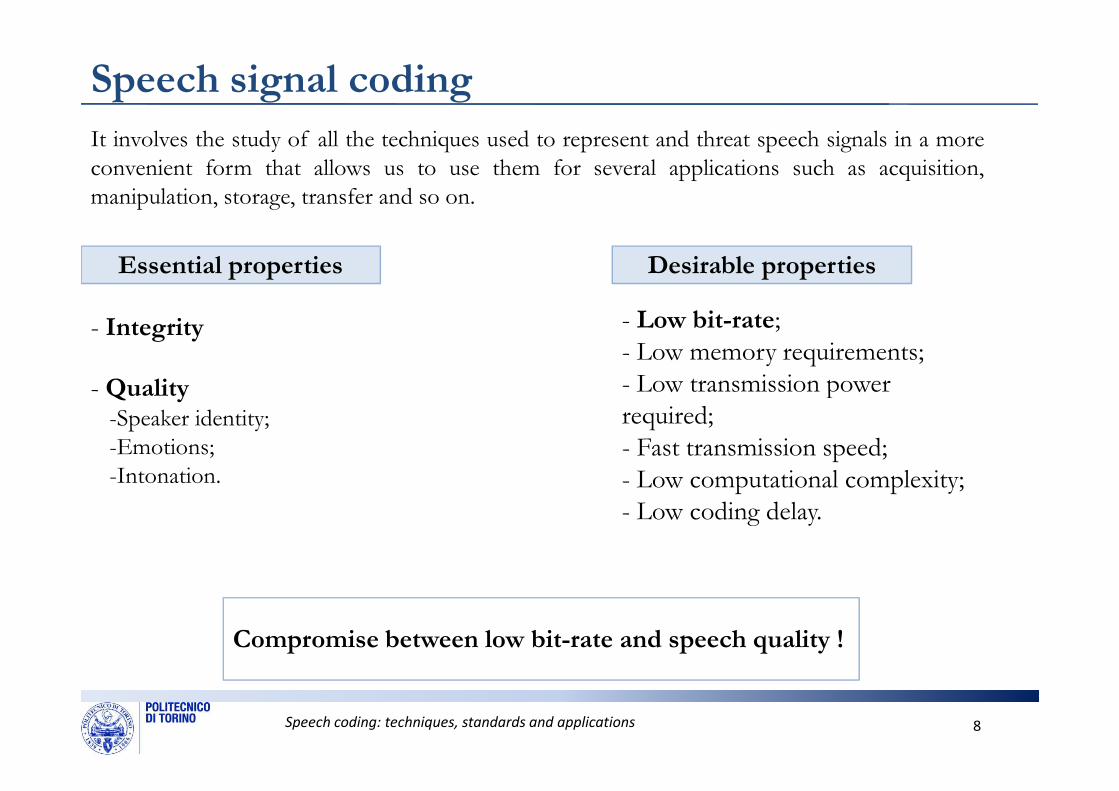
Speech signal coding

It involves the study of all the techniques used to represent and threat speech signals in a more

convenient form that allows us to use them for several applications such as acquisition,

manipulation, storage, transfer and so on.

Essential properties Desirable properties

- Integrity

- Quality

- Low bit-rate;- Low memory requirements;- Low transmission power


- Quality-Speaker identity;

-Emotions;

-Intonation.

- Low transmission power required;- Fast transmission speed;- Low computational complexity; - Low coding delay.

Compromise between low bit-rate and speech quality !

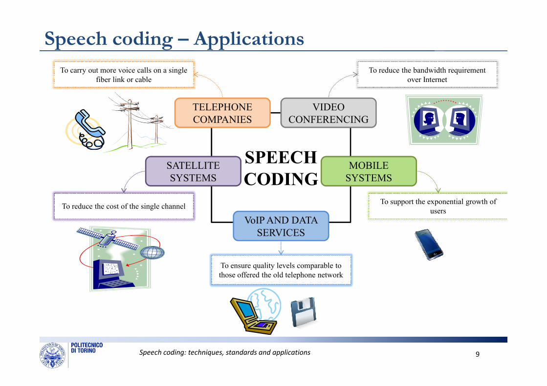
Speech coding – Applications

SPEECH

CODING

To carry out more voice calls on a single

fiber link or cable

TELEPHONE

COMPANIES

MOBILE

SYSTEMS

To reduce the bandwidth requirement

over Internet

VIDEO

CONFERENCING

SATELLITE

SYSTEMS


To support the exponential growth of

users

To ensure quality levels comparable to

those offered the old telephone network

VoIP AND DATA

SERVICES

To reduce the cost of the single channel

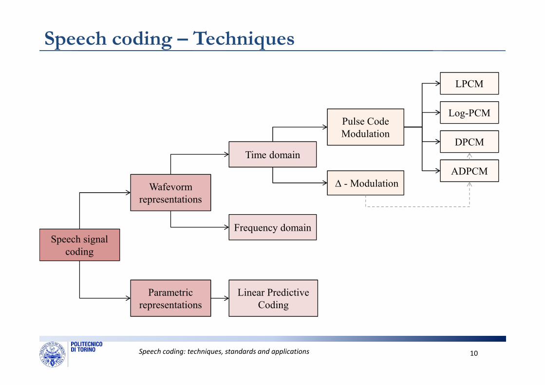
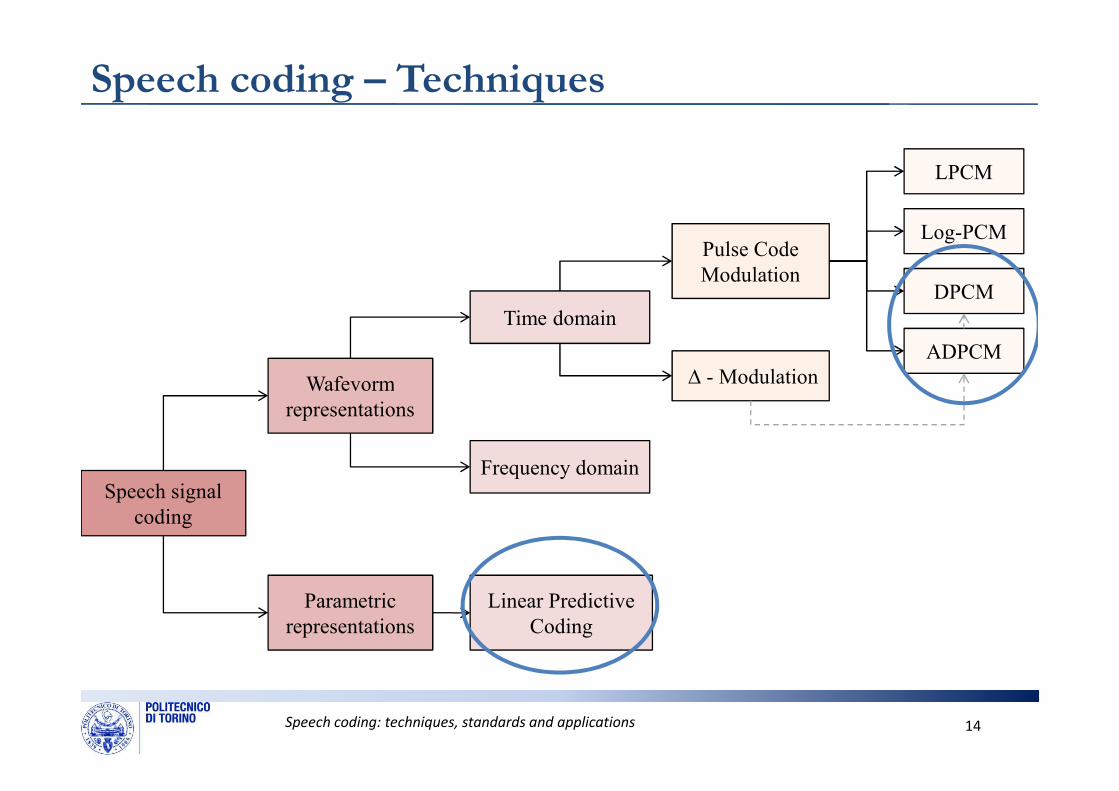
Speech coding – Techniques

Wafevorm

Time domain

Pulse Code

Modulation

Log-PCM

DPCM

ADPCM

∆ - Modulation

LPCM


Wafevorm

representations

Parametric

representations

Frequency domain Speech signal

coding

Linear Predictive

Coding

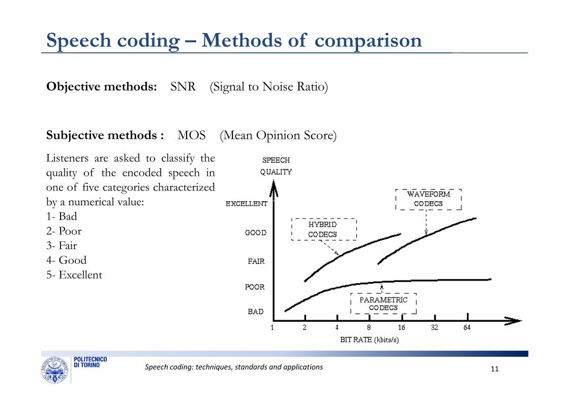
Speech coding – Methods of comparison

Objective methods: SNR (Signal to Noise Ratio)

Subjective methods : MOS (Mean Opinion Score)

Listeners are asked to classify the

quality of the encoded speech in

one of five categories characterized

by a numerical value:


by a numerical value:

1- Bad

2- Poor

3- Fair

4- Good

5- Excellent

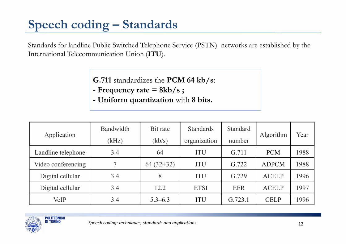
Speech coding – Standards

Standards for landline Public Switched Telephone Service (PSTN) networks are established by the

International Telecommunication Union (ITU).

G.711 standardizes the PCM 64 kb/s:- Frequency rate = 8kb/s ;

- Uniform quantization with 8 bits.


ApplicationBandwidth

(kHz)

Bit rate

(kb/s)

Standards

organization

Standard

numberAlgorithm Year

Landline telephone 3.4 64 ITU G.711 PCM 1988

Video conferencing 7 64 (32+32) ITU G.722 ADPCM 1988

Digital cellular 3.4 8 ITU G.729 ACELP 1996

Digital cellular 3.4 12.2 ETSI EFR ACELP 1997

VoIP 3.4 5.3–6.3 ITU G.723.1 CELP 1996

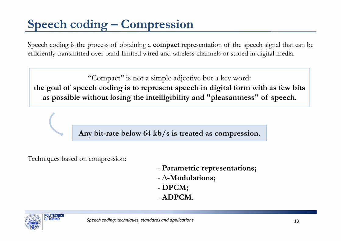
Speech coding – Compression

Speech coding is the process of obtaining a compact representation of the speech signal that can be

efficiently transmitted over band-limited wired and wireless channels or stored in digital media.

“Compact” is not a simple adjective but a key word: the goal of speech coding is to represent speech in digital form with as few bits

as possible without losing the intelligibility and "pleasantness" of speech.


Any bit-rate below 64 kb/s is treated as compression.

Techniques based on compression:

- Parametric representations;

- ∆-Modulations;

- DPCM;

- ADPCM.

Speech coding – Techniques

Wafevorm

Time domain

Pulse Code

Modulation

Log-PCM

DPCM

ADPCM

∆ - Modulation

LPCM


Wafevorm

representations

Parametric

representations

Frequency domain Speech signal

coding

Linear Predictive

Coding

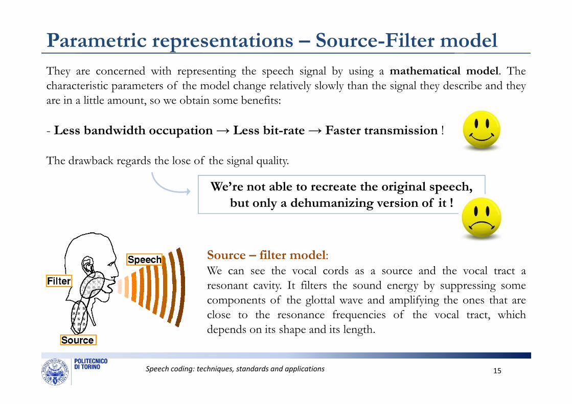
Parametric representations – Source-Filter model

They are concerned with representing the speech signal by using a mathematical model. The

characteristic parameters of the model change relatively slowly than the signal they describe and they

are in a little amount, so we obtain some benefits:

- Less bandwidth occupation → Less bit-rate → Faster transmission !

The drawback regards the lose of the signal quality.

We’re not able to recreate the original speech,

but only a dehumanizing version of it !


but only a dehumanizing version of it !

Source – filter model:We can see the vocal cords as a source and the vocal tract a

resonant cavity. It filters the sound energy by suppressing some

components of the glottal wave and amplifying the ones that are

close to the resonance frequencies of the vocal tract, which

depends on its shape and its length.

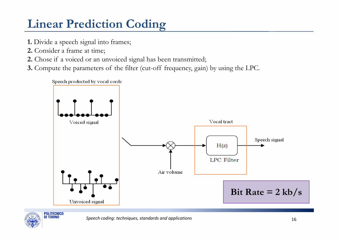
Linear Prediction Coding

1. Divide a speech signal into frames;

2. Consider a frame at time;

2. Chose if a voiced or an unvoiced signal has been transmitted;

3. Compute the parameters of the filter (cut-off frequency, gain) by using the LPC.


Bit Rate = 2 kb/s

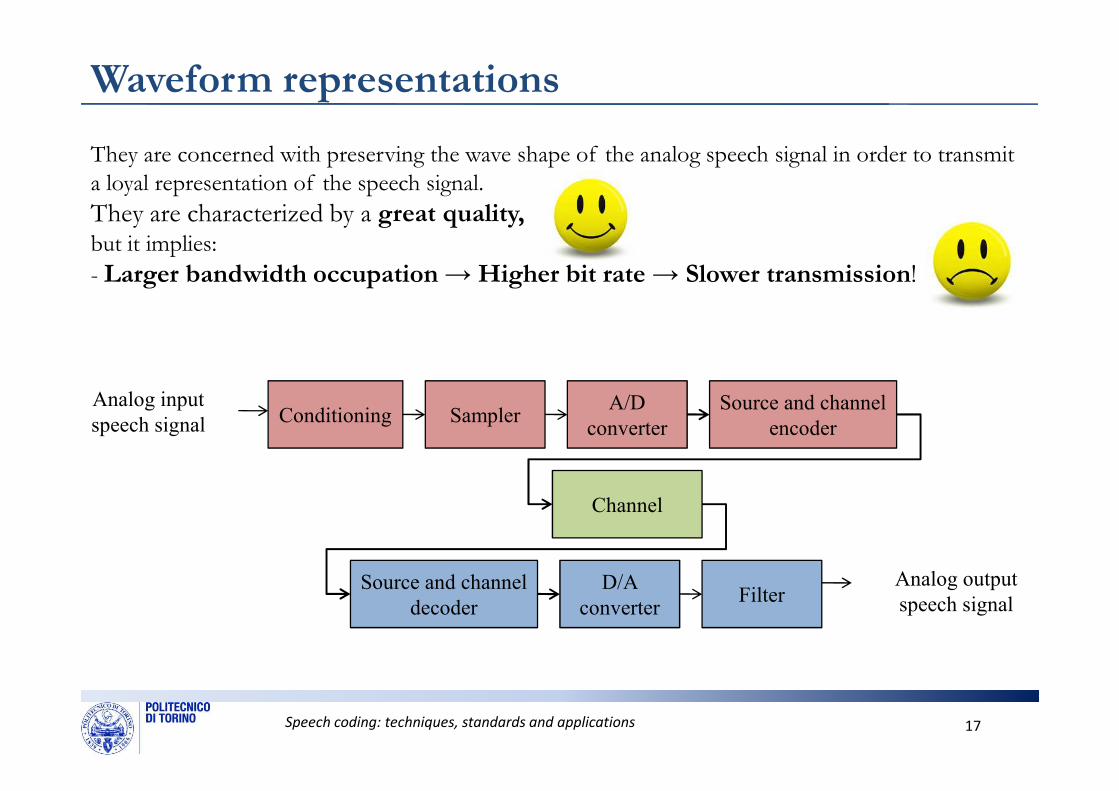
Waveform representations

They are concerned with preserving the wave shape of the analog speech signal in order to transmit

a loyal representation of the speech signal.

They are characterized by a great quality,but it implies:

- Larger bandwidth occupation → Higher bit rate → Slower transmission!

A/D Source and channelAnalog input


Conditioning SamplerA/D

converter

Source and channel

encoder

Source and channel

decoder

D/A

converterFilter

Channel

Analog input

speech signal

Analog output

speech signal

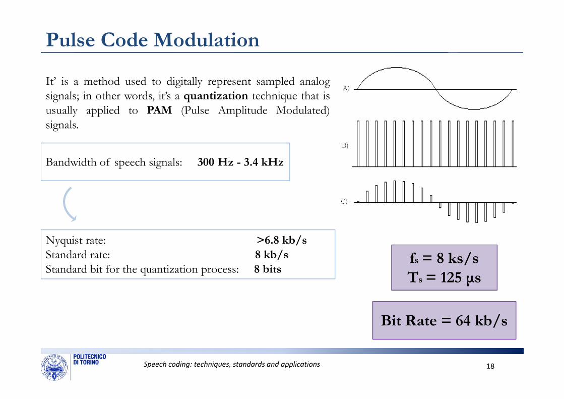
Pulse Code Modulation

It’ is a method used to digitally represent sampled analog

signals; in other words, it’s a quantization technique that is

usually applied to PAM (Pulse Amplitude Modulated)

signals.

Bandwidth of speech signals: 300 Hz - 3.4 kHz


fs = 8 ks/s

Ts = 125 µs

Bit Rate = 64 kb/s

Nyquist rate: >6.8 kb/s

Standard rate: 8 kb/s

Standard bit for the quantization process: 8 bits

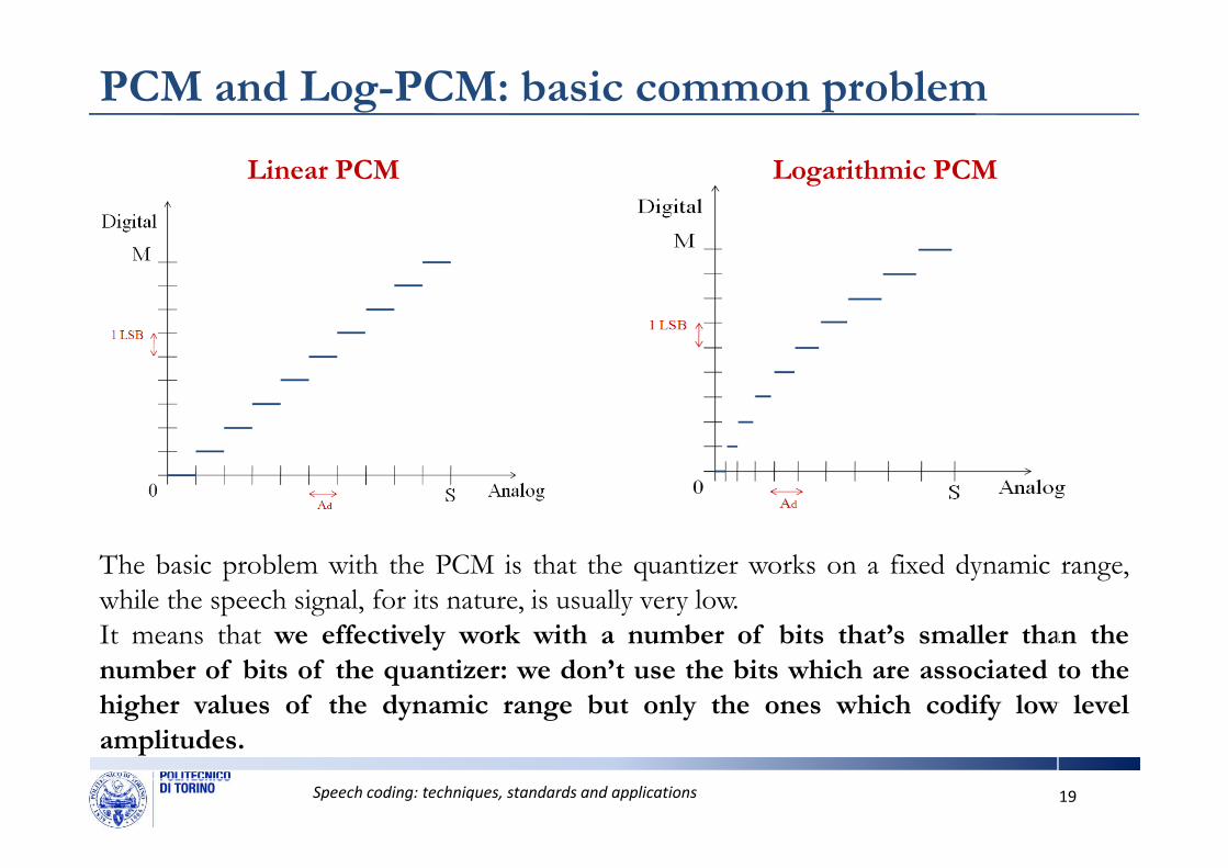
PCM and Log-PCM: basic common problem

Linear PCM Logarithmic PCM


The basic problem with the PCM is that the quantizer works on a fixed dynamic range,while the speech signal, for its nature, is usually very low.It means that we effectively work with a number of bits that’s smaller than the

number of bits of the quantizer: we don’t use the bits which are associated to the

higher values of the dynamic range but only the ones which codify low level

amplitudes.

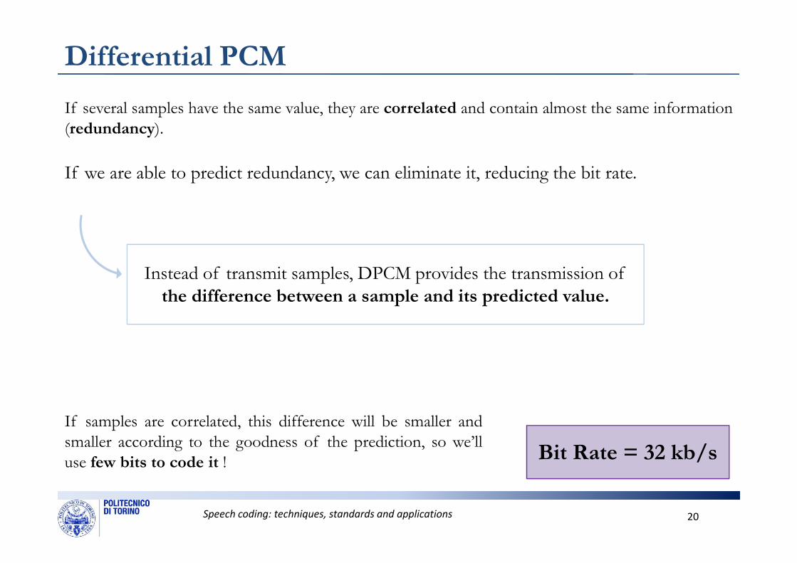
Differential PCM

If several samples have the same value, they are correlated and contain almost the same information

(redundancy).

If we are able to predict redundancy, we can eliminate it, reducing the bit rate.

Instead of transmit samples, DPCM provides the transmission of


Instead of transmit samples, DPCM provides the transmission ofthe difference between a sample and its predicted value.

If samples are correlated, this difference will be smaller and

smaller according to the goodness of the prediction, so we’ll

use few bits to code it ! Bit Rate = 32 kb/s

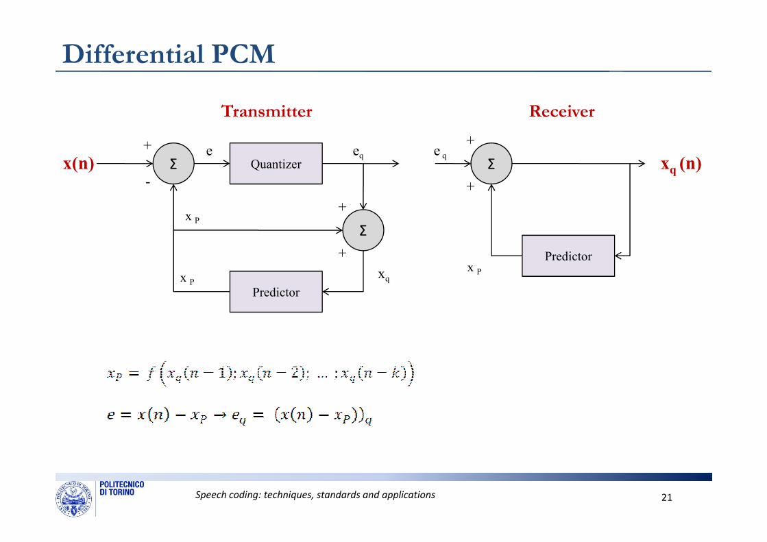
Differential PCM

Quantizerx(n) Σ

Σ

e

x

-

+

+

+

x P

eq

x

Predictor

Σ

+

+

xq (n)

x P

e q

Receiver Transmitter


Predictor

x Pxq

x P

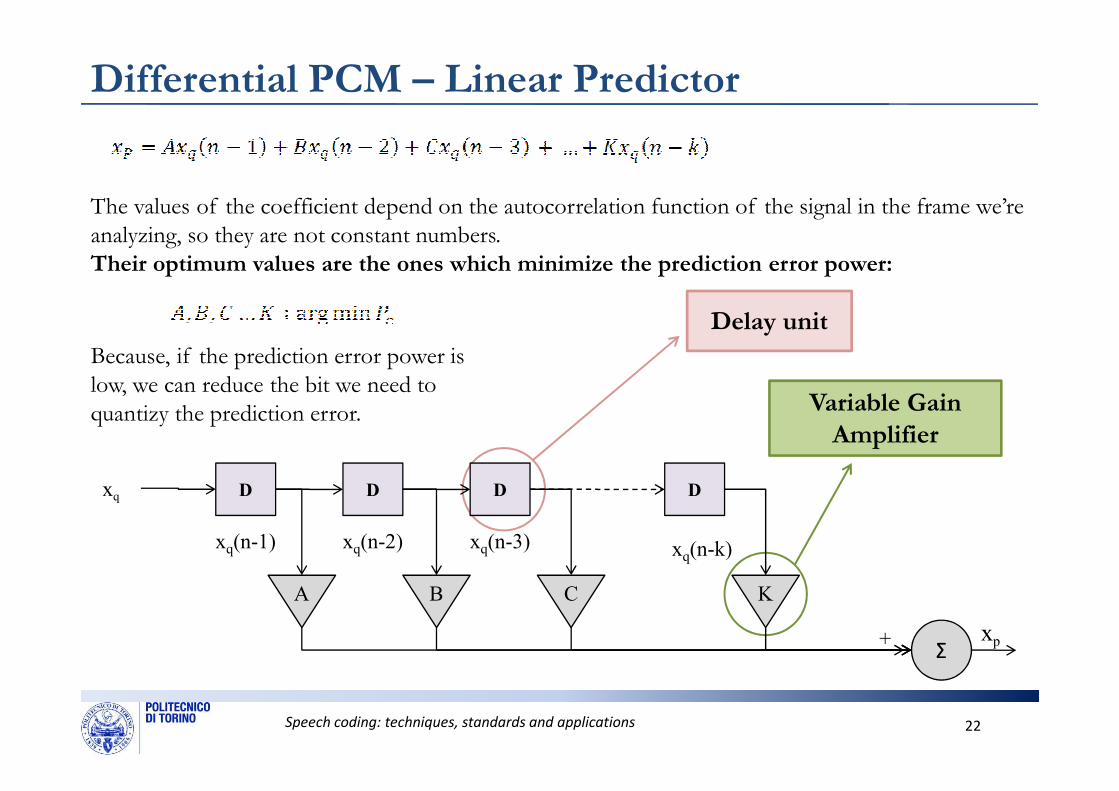
Differential PCM – Linear Predictor

The values of the coefficient depend on the autocorrelation function of the signal in the frame we’re

analyzing, so they are not constant numbers.

Their optimum values are the ones which minimize the prediction error power:

Because, if the prediction error power is

low, we can reduce the bit we need to

Delay unit

Variable Gain


low, we can reduce the bit we need to

quantizy the prediction error. Variable Gain

Amplifier

Σ+

xq D D D

xq(n-1)

D

xq(n-2) xq(n-k)xq(n-3)

xp

A B C K

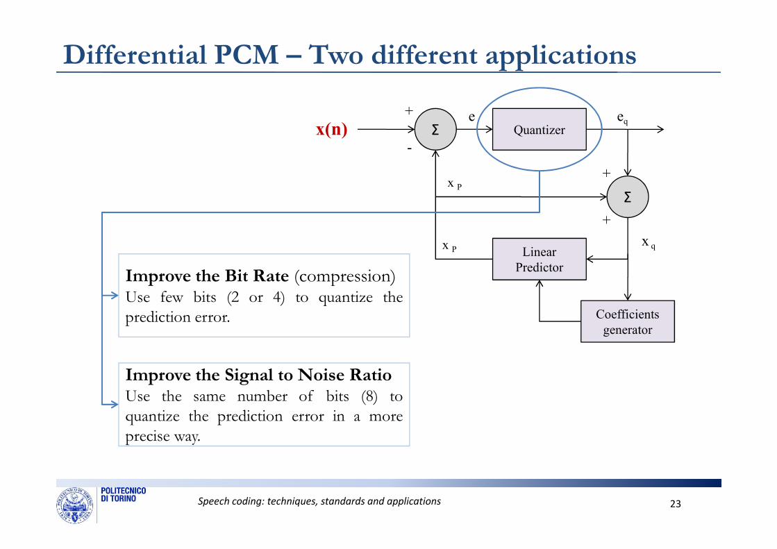
Differential PCM – Two different applications

Quantizerx(n) Σ

Linear

Predictor

Σ

e

x P

-

+

+

+

x P

eq

x q

Improve the Bit Rate (compression)


Coefficients

generator

Improve the Bit Rate (compression)Use few bits (2 or 4) to quantize the

prediction error.

Improve the Signal to Noise RatioUse the same number of bits (8) to

quantize the prediction error in a more

precise way.

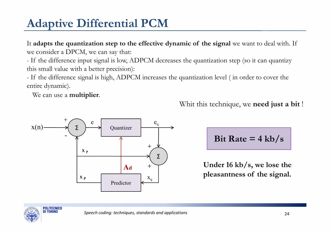
Adaptive Differential PCM

++

It adapts the quantization step to the effective dynamic of the signal we want to deal with. If

we consider a DPCM, we can say that:

- If the difference input signal is low, ADPCM decreases the quantization step (so it can quantizy

this small value with a better precision):

- If the difference signal is high, ADPCM increases the quantization level ( in order to cover the

entire dynamic).

We can use a multiplier.

Whit this technique, we need just a bit !


Quantizerx(n) Σ

Predictor

Σ

x P

-

+

+

+

x P

Ad

QuantizerΣ

Predictor

Σ

e

x P

-

+

+

+

x P

eq

xq

Under 16 kb/s, we lose the

pleasantness of the signal.

Bit Rate = 4 kb/s

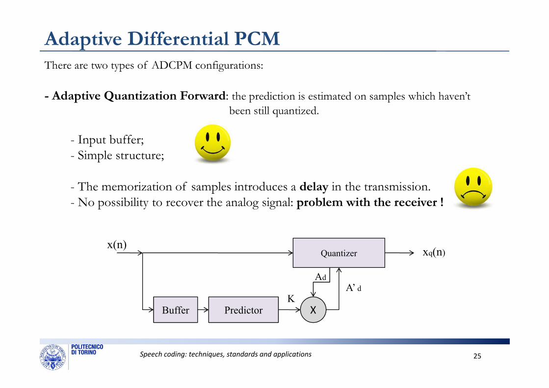
Adaptive Differential PCMThere are two types of ADCPM configurations:

- Adaptive Quantization Forward: the prediction is estimated on samples which haven’t

been still quantized.

- Input buffer;- Simple structure;

- The memorization of samples introduces a delay in the transmission.


- No possibility to recover the analog signal: problem with the receiver !

Buffer

Quantizer xq(n)

A’ d

Predictor

x(n)

X

K

Ad

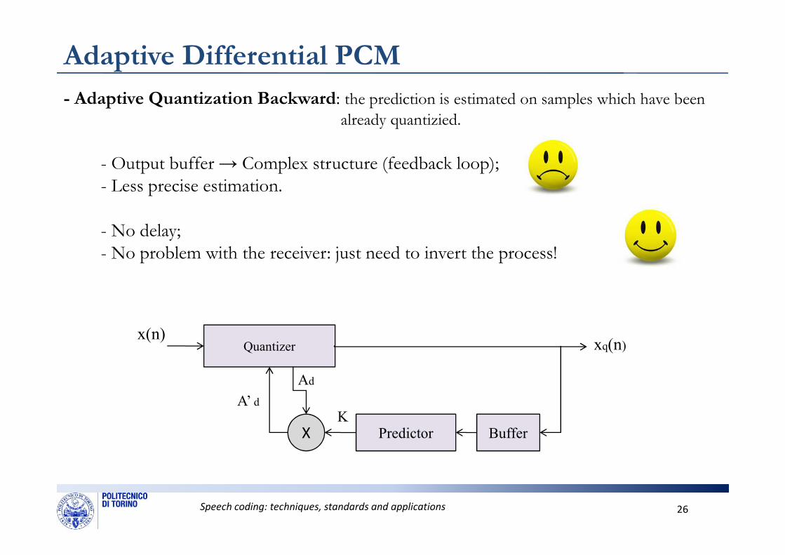
Adaptive Differential PCM

- Adaptive Quantization Backward: the prediction is estimated on samples which have been

already quantizied.

- Output buffer → Complex structure (feedback loop);- Less precise estimation.

- No delay;- No problem with the receiver: just need to invert the process!


BufferG

Quantizer

A’ d

Predictor

x(n)xq(n)

X

K

Ad

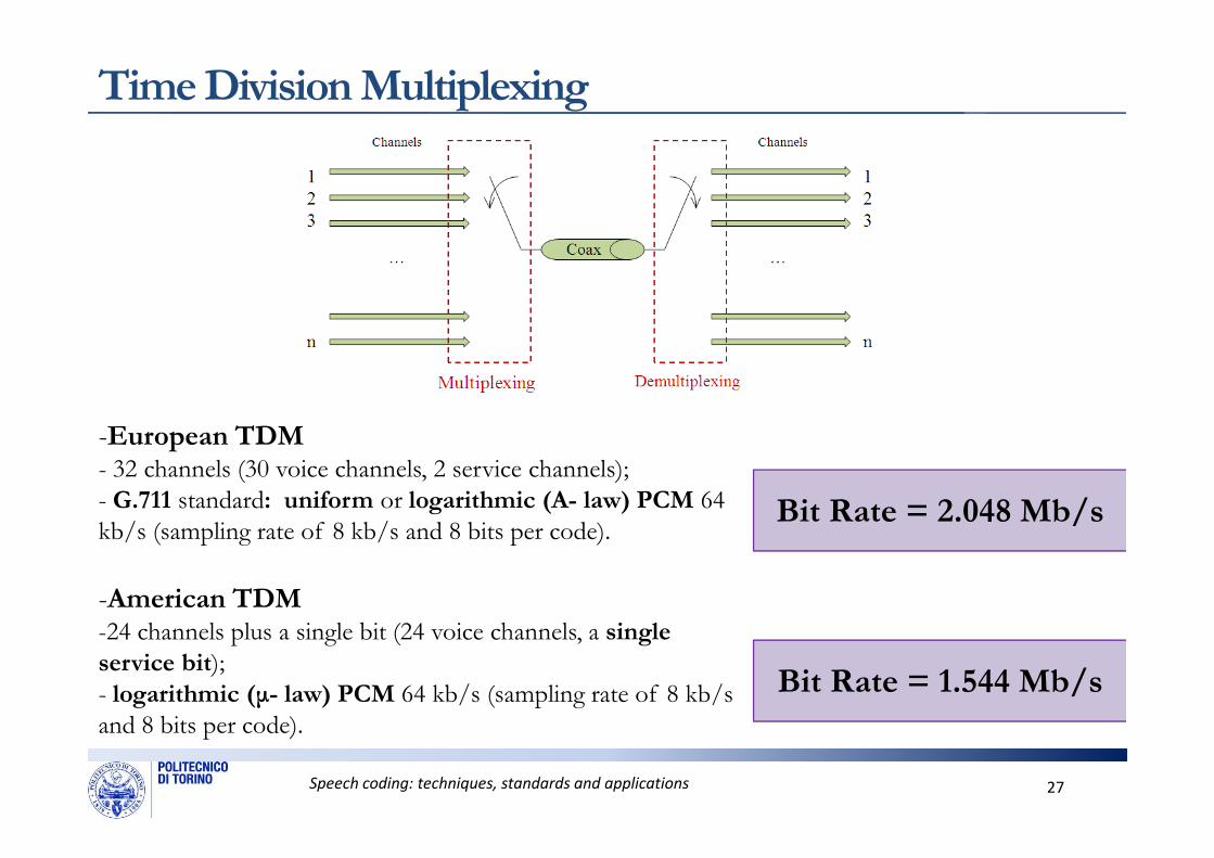
Time Division Multiplexing

-European TDM


-European TDM- 32 channels (30 voice channels, 2 service channels);

- G.711 standard: uniform or logarithmic (A- law) PCM 64

kb/s (sampling rate of 8 kb/s and 8 bits per code).

-American TDM-24 channels plus a single bit (24 voice channels, a single

service bit);

- logarithmic (µ- law) PCM 64 kb/s (sampling rate of 8 kb/s

and 8 bits per code).

Bit Rate = 2.048 Mb/s

Bit Rate = 1.544 Mb/s

ReferencesTexts:

•L.R. Rabiner & R. W. Schafer, Digital Processing of Speech Signals, Prentice-Hall, 1978. ISBN 0-13213603-1.

•D. Del Corso, Elettronica per Telecomunicazioni, McGraw-Hill, 2002. ISBN 88-386-0832-6.

•Jerry D. Gibson, Digital Compression for Multimedia: Principles and Standards, Elsevier Science (USA), 1998. ISBN

1-55860-369-7.

•Wiley Encyclopedia of Telecommunications, John Wiley & Sons, 2003. ISBN 978-0-471-36972-1.

Articles and slides downloaded from web (in May 2014):

•M. Hasegawa-Johnson & A. Alwan, Speech Coding: Fundamentals and Applications, University of Illinois at Urbana.


•M. Hasegawa-Johnson & A. Alwan, Speech Coding: Fundamentals and Applications, University of Illinois at Urbana.

(http://www.seas.ucla.edu/spapl/paper/mark_eot156.pdf )

•J. D. Gibson, Speech Coding Methods, Standards, Applications, University of California at Santa Barbara.

(http://vivonets.ece.ucsb.edu/casmagarticlefinal.pdf )

•D. Tipper, Digital Speech Processing, University of Pittsburgh

( www.pitt.edu/~dtipper/2720/2720_Slides7.pdf )

•D. P. W. Ellis, An introduction to signal processing for speech, Columbia University, 2008.

•It’s a chapter of the book by Hardacastle William J., The Handbook of Phonetic Sciences, edited by Wiley-Blackwell.

(http://academiccommons.columbia.edu/catalog/ac%3A144483 )

•P. Cummiskey, Adaptive Quantization in DPCM Coding of Speech, The Bell System Technical Journal (volume 52,

issue 7, pages 1105-1118), 1973.

(http://www.alcatel.hu/bstj/vol52-1973/articles/bstj52-7-1105.pdf )

Thank for your attention!


speech coding: techniques, standards and applications · it involves the study of the techniques we...

Documents