soil moisture variability in a temperate deciduous forest ...rvd/pub/ees_2014.pdf · insights from...

THEMATIC ISSUE

Soil moisture variability in a temperate deciduous forest:insights from electrical resistivity and throughfall data

Yuteng Ma • Remke L. Van Dam •

Dushmantha H. Jayawickreme

Received: 1 December 2013 / Accepted: 15 May 2014 / Published online: 4 June 2014

� Springer-Verlag Berlin Heidelberg 2014

Abstract In deciduous forests, soil moisture is an important

driver of numerous physical, microbial, and biogeochemical

processes. Therefore, characterizing the interactions between

vegetation and soil moisture is critical to forecast long-term

water resources and ecosystem health. However, these inter-

actions are difficult to measure, both in time and space.

Recent studies have shown the ability of electrical resistivity

imaging (ERI) to characterize the spatial and temporal

dynamics of soil moisture at a range of scales. However, no

study has yet attempted to use ERI to describe spatiotemporal

variability of soil water in relation to vegetation structure and

throughfall. In this study, at a mature forest site in Michigan,

USA, we captured spatial and temporal dynamics of soil

moisture using weekly ERI measurements augmented with

throughfall and soil temperature measurements, and a detailed

vegetation survey for five adjacent quadrats. Our results show

that throughout the growing season, the soil moisture gradu-

ally declined despite strong variations in cumulative monthly

rainfall. This decline was occasionally halted, but not

reversed, during weeks with high precipitation. Spatial vari-

ability of electrical resistivity and soil moisture was not

related to soil temperature differences but showed a strong

correlation with canopy variables.

Keywords Electrical resistivity � Deciduous forests �Forest ecology � Soil moisture � Throughfall

Introduction

The temperate-climate deciduous forests with four distinct

seasons are a common vegetation type in the northern

hemisphere (Hansen et al. 2000; Wen 1999; Keddy 1996).

With world’s population relying on forests for a range of

natural products and ecosystem services, it is critical that

these systems are properly understood and managed

(McElrone et al. 2013). Previous work has shown how

changes in precipitation, temperature, and wind may have

important consequences for the type and density of trees

(e.g., Reed and Desanker 1992; McKenney-Easterling

2000). Moreover, changes in CO2 concentration have been

shown to affect plant water demand and the soil water

balance of temperate forests (Schafer et al. 2002). In this

complex system, soil moisture is both an indicator and a

driver of change. Therefore, understanding the spatial and

temporal dynamics of near-surface soil moisture is a crit-

ical endeavor (Asbjornsen et al. 2011; Peng et al. 2013).

However, monitoring and quantifying soil water fluxes at

relevant spatial scales remains difficult because of the

above- and belowground heterogeneities inherent to forest

ecosystems.

Soil moisture content varies temporally as a result of

soil water inflow (precipitation and snow melt) and outflow

(root water uptake, evaporation, and deep drainage) dif-

ferences, driven by seasonal and stochastic weather events.

Soil moisture content also varies spatially because of soil

texture, vegetation canopy, litter density, root distribution,

and other landscape heterogeneities (e.g., Wilson et al.

2000; Griffiths et al. 2009; Xu et al. 2013; He et al. 2014).

Y. Ma � R. L. Van Dam (&)

Department of Geological Sciences, Michigan State University,

288 Farm Lane, East Lansing, MI 48824, USA

e-mail: [email protected]

R. L. Van Dam

Institute for Future Environments, Queensland University of

Technology, Gardens Point Campus, 2 George Street, Brisbane,

QLD 4000, Australia

D. H. Jayawickreme

Department of Geography, Bridgewater State University,

Bridgewater, MA 02325, USA

123

Environ Earth Sci (2014) 72:1367–1381

DOI 10.1007/s12665-014-3362-y

Over the years, different methods have been proposed to

assess the influence of these heterogeneities on soil water

(e.g., Breda et al. 2006; Wang et al. 2013). However,

integrating the data from these different methods and

quantifying the collective influence of multiple variables

on spatiotemporal soil water dynamics remains difficult.

In forests, a substantial portion of the precipitation may be

lost due to canopy interception and subsequent canopy

evaporation. The fraction of precipitation that reaches the

ground as stemflow or throughfall is important for soil water

balance and catchment hydrology (Bryant et al. 2005),

nutrient cycling (Michalzik et al. 2001), soil respiration

(Borken et al. 2006), and a range of microbial and biogeo-

chemical processes (Schliemann and Bockheim 2014). The

throughfall fraction, which is a critical component of the soil

water balance, depends on among others the canopy storage

capacity, precipitation intensity and duration, and atmo-

spheric variables such as wind and relative humidity that

influence evaporation rates (e.g., Klaassen 2001; Bryant

et al. 2005). Prior studies of throughfall variability have

shown that canopy interception decreases with distance from

tree stems (Johnson 1990). However, in a detailed study

using randomly spaced rain gauges in a deciduous forest,

Carlyle-Moses et al. (2004) found that the effect of stand

variability on throughfall was insignificant for larger pre-

cipitation events ([5 mm). Similarly, other studies have

looked at canopy attributes of different species and conse-

quent influence on throughfall fractions (e.g., Crockford and

Richardson 2000; Bryant et al. 2005). However, these studies

have rarely explored the influence of throughfall on soil

moisture development in the near surface, which is perhaps

the most important for understanding the aspects of forest

hydrology and biogeochemistry.

Soil moisture measurements have traditionally been

taken using gravimetric measurements of physical soil

samples. Such measurements provide accurate data, but are

time-consuming, invasive, and offer limited temporal and

spatial resolution. To overcome these limitations, time-

domain reflectometry (TDR) equipment, neutron probes,

and tensiometers are now frequently used (Breda et al.

1995; Wullschleger et al. 1998). These are useful methods

to obtain time series of soil water content, although

drawbacks include their invasive nature, limited spatial

sensitivity, susceptibility to errors resulting from poor

sensor-soil contact, and the need for multiple sensors when

soil moisture patterns over even modest field scales need to

be described.

In recent years, electrical resistivity imaging (ERI) has

become a popular method to study spatial and temporal

variability of soil properties (Jayawickreme et al. 2014). It

has been used for soil moisture assessment (e.g., Zhou et al.

2001; Michot et al. 2003), soil temperature studies (Pepin

and Livingston 1995; Musgrave and Binley 2011), and soil

structure and texture exploration (Omonode and Vyn 2006;

Lusch et al. 2009; Chaplot et al. 2010; Basso et al. 2012).

Furthermore, ERI is increasingly used to study the long-

term impacts of land-use conversions (Jayawickreme et al.

2011; Ahmed et al. 2012; Nosetto et al. 2013), agricultural

water management (Islami et al. 2011; Garre et al. 2013),

and to monitor water content in shallow bedrock (Nijland

et al. 2010; Yamakawa et al. 2012). A few recent studies

have also successfully used ERI to assess the relationships

between vegetation variables and soil moisture (Garcia-

Montiel et al. 2008; Robinson et al. 2012). However, no

study has yet attempted to utilize ERI to describe spatio-

temporal variability of soil water in relation to vegetation

structure and throughfall.

The primary objective of this work is to improve our

understanding of soil plant dynamics in temperate-climate

deciduous forests, with a focus on both seasonal change

and spatial variability in soil water content. In particular,

we explore whether the spatial pattern of soil water remains

the same during growing season and whether spatial vari-

ability of soil water is correlated to vegetation structure and

throughfall; we do not explicitly consider stemflow and the

role of plant litter and associated evaporation. To answer

these questions, we studied the growing season (May–

November) soil moisture patterns along with several key

vegetation and water balance attributes including stand

distribution and density, tree basal area, the leaf area index

(LAI), precipitation, and throughfall in a mature forest plot

in Michigan, USA.

Study site and methods

The study site is a patch of deciduous trees in central

Lower Michigan on a glacial till plane with nearly flat

topography (Fig. 1). The forest patch is laterally extensive

in an east–west direction but bordered to the south by a

recent clear-cut and to the north by a grassland. A north-

east- to southwest-oriented transect, 64.5 m in length and

with minimal topographic variations, was used for soil

water measurements with ERI (Fig. 2); the transect

extended another 60 m (40 electrodes) in the northeast

direction in the grassland (Jayawickreme et al. 2010), but

was not used for this study. Soil texture observations from

several boreholes along the transect show that the top

40–60 cm consists of clay loam, and is underlain primarily

by medium- to fine-grained sand, with porosities of 0.47

and 0.39, respectively (Jayawickreme et al. 2008). The

water table fluctuates between 3 and 4 m below the surface,

with highest water levels occurring before the onset of

active photosynthesis in early spring, and lowest water

levels in late fall around leaf senescence (Jayawickreme

et al. 2010).

1368 Environ Earth Sci (2014) 72:1367–1381

123

Vegetation structure

The forest consists of randomly distributed mostly mature

trees ([30 years old) dominated by sugar maple (Acer

saccharum). To characterize the vegetation structure at the

study site, a detailed vegetation survey was conducted in

June 2013 following standard protocols (e.g., Montgomery

and Chazdon 2001). Eight quadrats measuring 9 9 9 m

were laid out sequentially as shown in Fig. 2; each quadrat

centered on one of the TIF/iButton locations described

below. In this study, we only use the results from 5

quadrats (quadrat 2–6; quadrat 1 was only partly covered

by resistivity image points and quadrats 7 and 8 were

affected by the forest–grassland boundary). We mapped the

location of each tree in the quadrats and measured the

diameter at breast height (DBH). Basal area (BA) was

derived from the DBH measurements and scaled to 1

hectare size for easy comparison with values typically

given in the literature (e.g., Wardle et al. 2004). Crown

area (CA) of each tree was estimated using the maximum

canopy extent in four radial directions. The exact heights of

trees at the site were not measured, but they were estimated

to range between 25 and 35 m. Similarly, Crown depth

(CD) was also characterized only qualitatively, with a high

CD corresponding to trees where the first leafed branch

occurs at a height lower than half the tree height. The

results from the survey are summarized in Table 1.

Leaf area index (LAI) is a measure of canopy foliage

density that is broadly defined as the amount of leaf area in

a canopy per unit ground area (Chen et al. 1997). LAI has

been recognized as a key descriptive variable of forest

ecosystems because of the significant role green leaves

play in many biophysical processes. It may also correlate

with light transmittance and with some aspects of inter-

ception and throughfall (Lovett et al. 1996; Crockford and

Richardson 2000; Montgomery and Chazdon 2001). For a

database of measurements (n = 187) for temperate decid-

uous broad-leaved forests from around the world, Asner

et al. (2003) reported LAI values ranging from 1.1 to

8.8 m2/m2, with a mean of 5.1 m2/m2. For this study, a

complete LAI survey was conducted using a Decagon LP-

80 instrument at the peak of the growing season in 2012,

with LAI values (1.8–5.2 m2/m2; average 4.4 m2/m2) that

fall within the range suggested by Asner et al. (2003).

Aboveground monitoring equipment

The climate data obtained from a Michigan Automated

Weather Network (MAWN) station, located approximately

Fig. 1 Location of field site in Michigan

Fig. 2 Detailed layout of the field site showing the location of the

resistivity electrodes, 9 9 9 m vegetation survey quadrats, soil and

environmental sensors, and trees. One tipping-bucket rain gauge was

placed in the forest (survey quadrat 4); the location of the identical

rain gauge in the adjacent grassland plot is not shown in this figure

Table 1 Results from the vegetation survey for each survey quadrat,

giving the number of trees, average diameter at breast height (DBH),

basal area (BA), and average crown area (CA); non-living trees were

included in the calculations of DBH and BA

Quadrat # Total

trees

# Dead

trees

High

CD

DBH (m),

average

BA

(m2/

ha)

CA (m2),

average

2 3 0 2 0.48 102.1 105.7

3 7 1 2 0.28 77.9 36.4

4 1 0 1 0.37 13.0 81.3

5 4 1 1 0.27 32.6 39.0

6 6 0 3 0.25 43.5 24.0

See Fig. 2 for locations of the trees

Environ Earth Sci (2014) 72:1367–1381 1369

123

1.5 km from the site, were augmented with additional

equipment installed on-site. Precipitation information was

obtained from a tipping-bucket rain gauge that was placed

in the grassland. Data loggers recorded the time of every

0.2 mm of rainfall, but suffered from a few outages so that

the data cover only part of the study period. However,

sufficient volume of data was available for the comparison

of data from the on-site tipping-bucket and MAWN

weather station and to analyze the effect of different types

of storms on interception and throughfall.

Canopy throughfall in forests is considered quite vari-

able; in previous research, this has been measured in var-

ious ways, including using troughs, funnels, and standard

rain gauges (e.g., Crockford and Richardson 2000). Here,

we used two approaches for measuring throughfall. To

study the effects of rainfall duration and intensity on

throughfall, we used a tipping-bucket rain gauge in the

forest (Fig. 2). This complements the tipping-bucket rain

gauge that measured un-intercepted rainfall in the adjacent

grassland. To study the effects of canopy interception on

the spatial variability of forest throughfall, we used a novel,

low-budget method (throughfall integrating funnel, TIF)

that measures cumulative rainfall (Dunkerley 2010). In this

method, precipitation is collected in a funnel and guided

over a calcium sulfate hemihydrate tablet (‘‘Plaster of

Paris’’). As water flows over the tablet, a small amount of

calcium sulfate dissolves and is removed from the tablet.

Because the weight loss associated with a single precipi-

tation event is small, this method cannot be used to

quantify individual events. In this study, we used the

method to quantify the cumulative rain and throughfall

during approximately 4-week-long intervals (‘‘tablet

periods’’).

A total of 24 TIFs were installed at the site, including

18 in the forest (Fig. 2). All funnels were located

*65 cm above the ground surface. The TIFs in the

grassland are above the vegetation canopy and therefore

measured cumulative precipitation. Immediately before

field installation, the tablets were oven-dried at 120 �C

for 24 h and weighed. After approximately 4-week

intervals, the tablets were replaced with new ones. The

removed tablets were again oven-dried for 24 h and

weighed. The weight loss recorded during the tablet

period is proportional to the volume of water that has

passed over the tablet during that time interval (Dun-

kerley 2010). To facilitate comparisons between differ-

ent tablets and periods of different lengths, the weight

losses were normalized by starting weights (fractional

weight loss) and scaled to 28-day periods. The

throughfall fraction is then obtained from these data by

comparing the weight losses of TIFs placed under the

forest canopy with the average of those in the grassland.

Belowground monitoring equipment

The study site was instrumented with a suite of equipment

to monitor soil properties (Fig. 2). For soil temperature

measurements, a multidepth array (5, 10, 20, 60, and

100 cm below the surface) of Thermochron iButton sensors

(model DS1922L with a resolution of 0.0625 �C and an

accuracy of 0.5 �C) was installed. Additionally, iButton

sensors were installed 5 cm below the surface along the

forest transect, at 4.5 m lateral spacing. The sensors were

programmed to log data every 2 h and were downloaded

once every few months. A groundwater observation well at

the site was used for water-level and groundwater tem-

perature measurements. Soil moisture capacitance probes

at 20 and 80 cm depths in one location in the forest were

used for comparisons with ERI moisture estimates (Fig. 2).

Soil electrical resistivity data for monitoring soil water

dynamics were collected using a permanent transect. One

of the primary reasons for permanent electrode arrays is the

better repeatability of measurements, which improves the

signal-to-noise ratio for time-lapse resistivity surveys. The

transect consisted of 44 graphite electrodes spaced 1.5 m

apart (Fig. 2). The graphite rods, with 12 mm diameter and

30 cm length, were installed in 2006; they were buried

flush with the surface but made no contact with the soil for

the top 10 cm. To maximize data collection efficiency and

limit electrode-to-cable connection problems, the elec-

trodes were permanently wired to a central take-out loca-

tion using insulated 24-gauge wire. This setup eliminated

electrode position errors and incorrect wiring or connec-

tivity problems. Subsequent to electrode installation, the

area surrounding the transect was only minimally disturbed

by field activity at the site.

Approach

The study period spanned the 2012 growing season from

May through November. Based on the climate data

obtained from the nearby weather station, the temperature

range during the study period was comparable to the long-

term average (Fig. 3). According to long-term precipitation

data for the region, mean monthly precipitation from May

through September varies between 75 and 85 mm, and is

slightly lower (*60 mm) in October and November. The

average annual rainfall for the region is approximately

760 mm/year. Compared to the long-term mean, 2012

weather data showed that the study period was not typical,

with drier conditions in June and July, close to normal in

August and September, and a wetter November (Fig. 3).

During the study period, 24 individual electrical resis-

tivity datasets were collected using an AGI SuperSting


123

(R8/IP) resistivity system with external switchbox and a

Wenner array configuration at approximately weekly

intervals (Fig. 3). Each dataset along the 44-electrode

transect in the forest had 301 image points distributed over

14 image depths (a-spacings ranged from 1.5 to 22 m). An

analysis of contact resistance data from six datasets (iden-

tified with green lines in Fig. 3) throughout the growing

season (n = 1,806) shows limited correlation with electrode

location or a-spacing, indicating consistent data quality. As

expected, the average contact resistance did increase during

the growing season as the soil dried. In this study, no repeat

measurements or reciprocal data were collected to limit the

overall survey time to less than 90 min. However, previous

work at this site has shown that data quality is very high with

less than 0.2 % of data failing a tight repeat error criterion of

1 % (Jayawickreme et al. 2010). These repeat errors did not

correlate with geometric factors or environmental variables

(e.g., precipitation events and air temperature). Reciprocal

data from a nearby site with similar soil type, comparable

setup, and data collection procedures had an average reci-

procal error of 0.33 % (n = 289 with a-spacings that ranged

from 0.75 to 13.5 m).

To obtain insight into the temporal dynamics at the site,

we analyzed the difference between individual datasets.

Different procedures for inverting time-lapse geophysical

data have been proposed (Miller et al. 2008) including

(a) using one inverted resistivity model as a base model for

subsequent datasets, (b) inverting the difference between

two apparent resistivity datasets, and (c) subtracting

resistivity models after inverting them separately. The first

approach with a base inversion and monitoring datasets is a

common method to obtain differences between two data-

sets. However, potential disadvantages include the large

impact of the choice of base dataset on the resulting dif-

ferences and the possibility of error propagation in datasets

with non-systematic data errors (Jayawickreme et al.

2010). Here, we used the third approach by inverting the

datasets independently and subtracting the resulting models

to obtain the difference. Potential drawbacks of this

approach include the non-uniqueness of individual inver-

sions and the possibility that small errors in the data mask

actual resistivity changes (Daily et al. 2005).

Prior to inversion, clear outliers were removed from the

resistivity datasets. This applied to less than 1 % per

dataset with an average of 0.3 % per dataset. The inver-

sions were performed using AGI 2D Earthimager software.

The initial inversion step involved calculating a forward

model based on the pseudosection resistivity distribution.

We used a finite-difference mesh with a width and height

of 0.5 m. The total mesh consisted of 129 by 22 rectangular

cells plus eight padding cells around the domain, except the

surface. We then used an iterative Occam l2-norm smooth

inversion (Constable et al. 1987). All inversions were

halted at the same iteration step, at RMS data misfit levels

ranging between 2.8 and 4.3 %. This procedure not only

provides a comparable heterogeneity in each resistivity

model but also improves the ability to compare the spatial

distribution of resistivity and water content over time. No

topographic correction was applied as the elevation dif-

ferences along the line were very small and had no sig-

nificant effect on the inversion results.

Temperature correction

The influence of temperature on measured apparent resis-

tivity can be removed using empirical models. A linear

Fig. 3 Climate variables for the field site, including mean daily air

temperature (red line) and daily precipitation during the experiment

(blue vertical bars); data were obtained from the MAWN weather

station at Hancock Turfgrass Research Center, located 1.5 km from

the field site (42.7110, -84.4760). Also shown is the mean daily

temperature based on a record from 1980 to 2009 for East Lansing

(black line). Green hatched lines indicate dates of tablet installation

and replacement, with gray horizontal lines indicating the total

rainfall for each of the tablet periods. The black vertical lines at the

top of the graph indicate ERI data collection days


123

model was used in this study to correct for the temperature

effect, similar to that in Jayawickreme et al. (2010).

According to Sen and Goode (1992), the resistivity at a

base (reference) temperature can be calculated using

qref

qt

¼ c T � Trefð Þ þ 1; ð1Þ

where qref is the resistivity at a reference temperature

(T = 25 �C) and qt is the measured resistivity at temper-

ature T. The fractional change in resistivity per unit change

in temperature, c, is constant over the temperature range of

interest. Based on the data for glacial till materials, we used

a value of 0.018 (Hayley et al. 2007; Jayawickreme et al.

2008).

Temperature corrections were performed after inverting

the resistivity data. For these corrections, we used tem-

perature readings obtained from the temperature iButton

loggers at depths of 20, 40, 60, and 100 cm (Fig. 4). One

reading, closest to the time of resistivity data collection,

was used for each depth. Temperature was assumed to be

constant at 10.25 �C at 10 m depth after Jayawickreme

et al. (2010). No spatial variability in soil temperature was

incorporated in this correction because average soil tem-

perature data from the iButtons at 5 cm depth (Fig. 2) show

only very minor variations between sensor locations.

Water content conversion

In order to understand soil moisture distribution in space

and its dynamics in time, the resistivity models obtained

through inversion and after correction for the temperature

effect need to be converted to water content. Although the

relationship between electrical resistivity and water content

is well known to be soil-specific, there have been a few

efforts in recent years to establish general pedotransfer

functions (e.g., Hadzick et al. 2011). In this study, we used

material-specific relationships between resistivity (q) and

water content (h) developed in laboratory experiments

(Jayawickreme et al. 2010). Based on the laboratory

results, most of the soil materials tested follow a power

function that can be expressed as S ¼ qs

q

� �m�1, where S is

the saturation (water content/porosity) and qs is the bulk

resistivity of soil at 100 % saturation. The m value was

estimated as 1.16 for sand and 0.67 for clay loam, and qs is

71.53 and 68.15 Xm, respectively (Jayawickreme et al.

2008). After inverted resistivities were corrected for the

temperature effect, the soil water content was calculated.

Soil moisture contents obtained using this procedure cor-

relate well with soil moisture values obtained using the

capacitance probes, but are slightly underestimated:

h(ERI) = 0.93 9 h(cp) ? 0.02 (Jayawickreme et al. 2010).

Results

Resistivity data

The ERI data collection interval allowed for the analysis of

long-term changes corresponding to the periods between

tablet swaps as well as shorter-duration soil water

dynamics. For the analysis of shorter-duration dynamics,

we categorized weeks as having high ([15 mm) or low (0–

5 mm) cumulative precipitation. Plots of resistivity change

between datasets were generated by calculating the percent

difference between (temperature-corrected) resistivity

models usingqnþ1�qn

qn

� �� 100, where qn?1 and qn are the

resistivity values from ending and starting models,

respectively.

During the 2 weeks with low cumulative precipitation at

the beginning of the growing season (Table 2), soil resis-

tivity shows a general increase, as would be expected

(Fig. 5). The week in early June (June 6–13) shows a lower

increase than the week in late June (June 27–July 3), even

though both weeks had B1 mm of water input. For weeks

with high cumulative precipitation (Table 2), the resistivity

response depended strongly on the time of the growing

season (early, mid, or late). During the week with 19.6 mm

of rainfall in early June (May 30–June 6), soil resistivity

shows a very limited decrease, except for a few small areas

near the surface (Fig. 6). The absence of a widespread

decline in resistivity in response to throughfall shows that

Fig. 4 Soil temperature measurements at different depths (0.2, 0.4,

0.6, and 1 m) during ERI data collection. Second-order polynomials

fitted to these data, and extended via a linear function to a constant

temperature at depth (see text), were used for temperature correction

of inverted resistivity models. The first three depths used for

temperature corrections are indicated with dotted horizontal lines


123

during the early growing season, the vegetative demand for

soil water outweighed the input from throughfall and

stemflow. In contrast, a similar cumulative precipitation

(17.5 mm) later in the growing season (August 30–Sep-

tember 6) caused the shallow soil resistivity to decrease

noticeably, although no change was evident below *0.5 m

depth (Fig. 6). The week in October with 39.6 mm of

cumulative precipitation triggered an even stronger nega-

tive response from the surface to about 0.5 m depth

(Fig. 6). This image also shows the initiation of lateral

resistivity heterogeneities where the negative resistivity

changes span the entire 2 m depth. The locations of most of

these heterogeneities also correlate with areas of minor

resistivity reductions following rainfall in early June

(Fig. 6 top panel).

Inverted resistivity models for the six dates during

which the throughfall tablets were installed or replaced

show a general increase in resistivity from early growing

season in late May until late September (Fig. 7). The

inverted models show some distinct lateral variability with

relatively high resistivity patches at *18.75 and *50 m

distance. There are also some areas with smaller-scale

lateral variability in resistivity, the dimensions of which

appear to change during the growing season. The resistivity

model for the last measurement on October 24 (Fig. 7)

shows a considerable resistivity reduction compared to the

earlier dates. This reduction can be attributed to the sig-

nificant rainfall (81 mm) between September 26 and

October 24 (Table 2). The influence of this rainfall was

accentuated by lower evaporative demand (lower temper-

atures), and fall senescence, which substantially reduced

the interception losses. In the October model, much of the

spatial variability that developed during the growing sea-

son has disappeared.

The first two-and-a-half months of the study period

(mid-May through July) were characterized by rainfall

quantities more than 50 % below average and relatively

high air temperatures. During this period, the resistivity

increased considerably, which corresponds to a distinct

decrease in soil moisture (Fig. 8). During the second half

of the growing season in July and August, rainfall amounts

were significantly higher with totals close to the mean

monthly precipitation for the region (Fig. 3). Thus, near-

surface resistivity occasionally dropped during weeks with

high cumulative rainfall (Fig. 6, center panel). Overall, and

despite the high rainfall, however, the soils continued to

lose moisture during the second half of the growing season

Fig. 5 Percent change in

resistivity for approximately

1-week time periods with low

cumulative precipitation from

June 6 to June 13 and from June

27 to July 3. For this and the

following figures, tick marks on

the horizontal axes correspond

to the boundaries of vegetation

quadrats 2–6 (Fig. 2). All data

shown in this and following

figures (Figs. 6, 7, 8, and 9)

have been temperature-

corrected

Table 2 Details of cumulative precipitation for selected low-

(0–5 mm) and high- ([15 mm) precipitation weeks discussed in the

text, and for the tablet swap periods

Start date End date Cumulative

precipitation

(mm)

Number

of days

Normalized

rainfall

(mm/day)

May 30 June 6 19.55 7 2.8

June 6 June 13 1.01 7 0.14

June 27 July 3 0 6 0

August 30 September 6 17.53 7 2.5

October 10 October 17 39.56 7 5.7

May 30 June 27 31.24 28 1.1

June 27 July 25 24.38 28 0.87

July 25 August 30 65.52 36 1.8

August 30 September 26 55.37 27 2.1

September 26 October 24 81.03 28 2.9


123

Fig. 6 Percent change in

resistivity for approximately

1-week time periods with high

cumulative precipitation from

May 30 to June 6, August 30 to

September 6, and October 10 to

October 17

Fig. 7 Inverted and

temperature-corrected

resistivity models of six ERI

datasets collected on days of

tablet installation and

replacement (see Fig. 3)


123

(Fig. 8). The soil water deficit recovered only after Sep-

tember, when plant water use started to decrease and major

rain events took place. The percent change in soil moisture

between two successive tablet periods is shown in Fig. 9. A

decrease in soil moisture indicates that the evapotranspi-

ration and possible soil water drainage exceeded the water

input from throughfall and stemflow for that period. This

series of images clearly shows that the largest changes in

soil moisture occurred early in the growing season during

the first two tablet periods (May 30 to June 27 and June 27

to July 25; Fig. 9). Despite a significant increase in

cumulative rainfall (Fig. 3), soil drying continued for the

next two tablet periods (July 25 to August 30 and August

30 to September 26; Fig. 9). These latter two periods had a

comparable amount of rainfall (65 and 55 mm, respec-

tively; Table 2), but the behavior was quite different with a

small but distinct near-surface soil moisture increase for

the third period from July 25 to August 30. The reduced

drying observed for the third and fourth periods compared

with the first two is likely a direct result of the increased

precipitation. It may be augmented, however, by a lower

plant water demand related to the lower daily mean tem-

perature. Another possibility is that at this time of the year

when the upper soil layer is already dry, the trees use more

water from near of below the water table. This was sug-

gested by Jayawickreme et al. (2008), who showed that the

effective rooting depth of these trees potentially extends to

at least 4 m below the surface during particularly dry

growing seasons. The situation changed for the last tablet

period when water content strongly increased (Fig. 9).

Vegetation structure

Results of the vegetation survey are given in Fig. 10 with

additional details in Table 1. The survey shows that along

the measurement line there are two distinct areas with a

clustering of trees (Fig. 10a). These clusters are separated

by an approximately 15-m-wide area with low tree density

(27–42 m). This zone encompasses all of quadrat 4 and

part of 5. The number of live trees in each quadrat varies

between 1 (quadrat 4) and 6 (quadrats 3 and 6). The basal

area depends on stem diameter (DBH) and is not neces-

sarily correlated with the number of trees (e.g., quadrat 2 in

Fig. 10b). Quadrat 6, close to the forest edge, has a high

number of trees but the basal area is relatively small. LAI

shows a clear high in quadrats 5 and 6, as does crown area

for quadrat 6. The low values for the LAI and crown area in

vegetation quadrat 3 (Fig. 10c) are surprising as this

Fig. 8 Volumetric water

content for the six dates of

tablet installation and

replacement


123

quadrat has a relatively large number of trees (Table 1).

However, it must be noted that there is not necessarily a

perfect correlation between stem and canopy measure-

ments because of, among other factors, encroachment of

tree canopies from outside the quadrats. Also, with the LAI

measurements in mid-morning, there may have been some

excess light that entered the forest from the southern

boundary.

Throughfall

As rainfall interception by forest canopies depends on a

large range of factors related to climatic conditions (e.g.,

rainfall duration and intensity, drop size, and wind speed)

and vegetation (e.g., leaf shape and inclination, and LAI), it

is difficult to make generalizations about interception los-

ses and throughfall rates, even for specific forests (Crock-

ford and Richardson 2000). However, it is well known that

for small events, a larger percentage of rainfall is inter-

cepted than for large events (e.g., Link et al. 2004). Once

the canopy storage capacity has been exceeded, for tree

species with downward pointing leaves, excess water will

drip off and fall to the ground. It is therefore understood

that throughfall rates are not linear with event size.

The tipping-bucket rain gauge in the grassland recorded

14 precipitation events during the study period, ranging

from 0.2 to 18 mm. Comparison of these data and with the

tipping-bucket rain gauge in the forest below the forest

canopy gave a forest throughfall fraction of 78 %

(Fig. 11a). There was little difference in this fraction

between events of varying amounts, with a linear rela-

tionship between event size and throughfall fraction

(R2 = 0.97). All events were of relatively short duration,

low intensity, and small size (amount). This likely kept all

events below the canopy storage capacity, resulting in the

linear relationship between event size and throughfall

fraction.

The smallest events in the dataset are not well repre-

sented in the tipping-bucket throughfall analysis. At very

low rainfall amounts, the signal-to-noise ratio becomes

very small and their overall effect cannot be established.

The analysis performed using the throughfall integrating

funnels has the potential to estimate the effect of these

small events, albeit not on an individual event basis. As the

Fig. 9 Percent change in water

content for the five tablet

periods. The anomaly around

29 m in some of the plots is due

to a bad data point in the

September 26 dataset


123

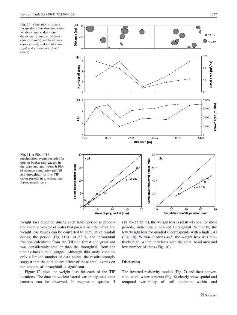
weight loss recorded during each tablet period is propor-

tional to the volume of water that passed over the tablet, the

weight loss values can be converted to cumulative rainfall

during the period (Fig. 11b). At 63 %, the throughfall

fraction calculated from the TIFs in forest and grassland

was considerably smaller than the throughfall from the

tipping-bucket rain gauges. Although this study contains

only a limited number of data points, the results strongly

suggest that the cumulative effect of these small events on

the amount of throughfall is significant.

Figure 12 plots the weight loss for each of the TIF

locations. The data show clear lateral variability, and some

patterns can be observed. In vegetation quadrat 3

(18.75–27.75 m), the weight loss is relatively low for most

periods, indicating a reduced throughfall. Similarly, the

low weight loss for quadrat 6 corresponds with a high LAI

(Fig. 10). Within quadrats 4–5, the weight loss was rela-

tively high, which correlates with the small basal area and

low number of trees (Fig. 10).

Discussion

The inverted resistivity models (Fig. 7) and their conver-

sion to soil water contents (Fig. 8) clearly show spatial and

temporal variability of soil moisture within and

Fig. 10 Vegetation structure

for quadrats 2–6 showing a tree

locations and scaled stem

diameters, b number of trees

(filled triangle) and basal area

(open circle), and c LAI (cross

sign) and crown area (filled

circle)

Fig. 11 a Plot of 14

precipitation events recorded in

tipping-bucket rain gauges in

the grassland and forest. b Plot

of average cumulative rainfall

and throughfall for five TIF

tablet periods in grassland and

forest, respectively


123

between the study quadrats. Similarly, spatial variability is

observed in the data on vegetation characteristics and

throughfall (Figs. 10, 12). In this section, we will address

the persistence of these spatial patterns throughout the

growing season, as well as the correlation between soil

moisture and the other measured variables.

Figure 13 presents the average water content below

each vegetation quadrat, for depth ranges of 0–50,

50–100, and 100–200 cm to emphasize different parts of

the root zone. The results show that at the beginning of

the growing season, the soil moisture contents were

highest, irrespective of the depth range. Soil moisture

distribution appears fairly constant across the array with

relatively small differences between vegetation quadrats.

At most times, quadrat 6 had the lowest water content

values along the array. The changes in water content

during tablet periods (Fig. 14) show a clear drying pattern

(negative change), except for the last period from Sep-

tember 26 to October 24. The changes throughout the

growing season are most significant for the 0- to 50-cm-

depth range (Fig. 14a). The smallest change along the

survey transect nearly always occurred in vegetation

quadrat 4 (between 27.75 and 36.75 m), which had the

lowest number of trees, the smallest basal area, and a

slightly higher throughfall volume (high TIF fractional

weight loss; Fig. 12). This suggests that the small and

slow resistivity response in this quadrat is driven by a

smaller soil water extraction by plants and the greater

throughfall volume, which likely kept the soil replenished

with moisture.

To compare soil moisture at different depths along the

measurement transect with data on throughfall and soil

temperature we used only the sensors located in the centers

of the five vegetation quadrats. Sensors located on the

quadrat edges (Fig. 2) were not included in these com-

parisons. The correlation between soil temperature (both

absolute and differenced between data collection periods)

and vegetation parameters and soil moisture did not pro-

duce statistically significant correlations. This was an

expected result based on the earlier observation of limited

spatial variability in soil temperature along the transect.

During the first 2 months of the growing season, the soil

dried relatively fast, especially in the shallow soil layers

(Fig. 14a). A comparison of soil moisture change and

normalized tablet weight loss for these months shows that

in quadrats with more throughfall, the drying is less pro-

nounced (Fig. 15a). This result is as expected, but the

correlations are relatively weak. This may be the result of

the previously discussed strong heterogeneity in through-

fall that is difficult to capture using the TIF method and

limited measurement locations. During the third and fourth

tablet periods, when soil moisture content changed rela-

tively little (Fig. 14), there is no correlation between tablet

weight loss and the soil moisture change (Fig. 15a). During

the final tablet period, strongest wetting is concentrated in

quadrats with less throughfall. This result may indicate that

in these quadrats the growing season moisture deficit was

most significant.

A quantitative comparison between soil moisture and

vegetation characteristics shows a strong negative corre-

lation with crown area (Fig. 15b) and LAI during the

growing season. This correlation between soil moisture and

canopy indicators was strongest at the start of growing

season, when quadrats with more canopy (high LAI or

large crown area) had distinctly lower soil moisture con-

tents. The slope of this correlation gradually dropped

throughout the growing season (although the correlation

coefficients remain strong), which suggests that the root

water uptake was uniform along the transect and uncorre-

lated with canopy structure. The final period from Sep-

tember 26 to October 24 at the end of the growing season,

which was characterized by high rainfall amounts (Fig. 2),

coincided with leaf fall-off. Higher throughfall quantities

along the transect resulted in disappearance of the corre-

lation between soil moisture and canopy indicators

(Fig. 15b), as would be expected. The lower depth intervals

showed comparable behavior, although the effect of can-

opy became less significant with depth. Analysis of the data

shows no strong correlation between DBH and the number

of trees with soil moisture distribution; this is no surprise as

these vegetation variables do not significantly impact

interception and throughfall.

Fig. 12 Tablet weight loss for

each of the TIF locations along

the survey transect. To enable

direct comparisons, the weights

have been normalized to correct

for different starting weights of

the tablets and scaled to 28-day

periods


123

0

0.1

0.2

0.3

0.4

9.75 27.75 45.75

So

il m

ois

ture

Distance (m)9.75 27.75 45.75

Distance (m)

9.75 27.75 45.75

Distance (m)

5/30 6/277/25 8/309/26 10/24

(a) (b) (c)

Fig. 13 Average ERI-derived soil moisture for vegetation survey quadrats 2–6 from a 0–50 cm, b 50–100 cm, and c 100–200 cm depth

-100

0

9.75 27.75 45.75

So

il m

ois

ture

ch

ang

e (%

)

Distance (m)

9.75 27.75 45.75

Distance (m)

9.75 27.75 45.75

Distance (m)

5/30-6/276/27-7/257/25-8/308/30-9/269/26-10/24

(a) (b) (c)

Fig. 14 Percent change in soil moisture between tablet periods for vegetation survey quadrats 2–6 from a 0–50 cm, b 50–100 cm, and

c 100–200 cm depth

Fig. 15 Comparison of soil moisture (averaged per quadrat), vege-

tation properties, and throughfall data. a Change in soil moisture in 5

vegetation quadrats versus tablet weight loss. To enable direct

comparisons, the weights were normalized to correct for different

starting weights of the tablets and scaled to 28-day periods. b Average

soil moisture in 5 vegetation quadrats versus crown area. Linear

regression lines (dashed) are given for datasets on May 30 (first and

wettest), September 26 (driest), and October 24 (last), and the average

(solid line). In both a and b, soil moisture from 0–50 cm was

averaged for each quadrat


123

Conclusions

This work presented a study of the effects of vegetation

structure on near-surface soil moisture, and its relation

with throughfall, in a temperate deciduous woodland. The

temporal dynamics of soil moisture monitored during the

growing season showed near-continuous drying. This was

especially the case early in the growing season when

precipitation was significantly below normal at the site.

However, this soil drying continued well into the second

half of the growing season when precipitation amounts

were substantially higher. During weeks with significant

precipitation amounts, only minor interruptions to this

drying trend were observed. In the early parts of the

growing season, even with substantial throughfall

amounts, no significant interruption to the drying occur-

red, likely as a result of high plant water consumption.

Later in the growing season, similar throughfall produced

more distinct wetting signatures. Based on the resistivity

data gathered, we also observed that with influxes of

precipitation during the growing season, significant spa-

tial heterogeneities in resistivity or soil moisture devel-

oped. These patterns in resistivity and soil moisture

correlated with some vegetation characteristics, in par-

ticular with the crown area of the trees and LAI. The

number of trees and DBH had no significant effect on the

distribution of soil moisture at the site. The spatial vari-

ability in soil moisture was also weakly correlated with

throughfall. The data presented in this paper provide

insights into the important relationships between vegeta-

tion characteristics of forests, including stand properties

and interception, and soil moisture that are still noticeably

absent in the literature.

Acknowledgments This research was funded by the US National

Science Foundation (NSF Grant EAR-0911642). Any opinions,

findings, and conclusions or recommendations expressed in this

publication are those of the authors and do not necessarily reflect the

views of the NSF. We acknowledge Agustin Brena, David Hyndman,

Anthony Kendall, Alex Kuhl, James Loop, and Ryan Nagelkirk for

field assistance and discussion of results. The manuscript benefited

from constructive comments by three anonymous reviewers.

References

Ahmed YAR, Pichler V, Homolak M, Gomoryova E, Nagy D,

Pichlerova M, Gregor J (2012) High organic carbon stock in a

karstic soil of the Middle-European Forest Province persists after

centuries-long agroforestry management. Eur J For Res

131:1669–1680

Asbjornsen H, Goldsmith GR, Alvarado-Barrientos MS, Rebel K,

Van Osch FP, Rietkerk M, Chen J, Gotsch S, Tobon C, Geissert

DR, Gomez-Tagle A, Vache K, Dawson TE (2011) Ecohydro-

logical advances and applications in plant–water relations

research: a review. J Plant Ecol 4:3–22

Asner GP, Scurlock JMO, Hicke JA (2003) Global synthesis of leaf

area index observations: implications for ecological and remote

sensing studies. Glob Ecol Biogeogr 12:191–205

Basso B, Fiorentino C, Cammarano D, Cafiero G, Dardanelli J (2012)

Analysis of rainfall distribution on spatial and temporal patterns

of wheat yield in Mediterranean environment. Eur J Agron

41:52–65

Borken W, Savage K, Davidson EA, Trumbore SE (2006) Effects of

experimental drought on soil respiration and radiocarbon efflux

from a temperate forest soil. Glob Change Biol 12:177–193

Breda N, Granier A, Barataud F, Moyne C (1995) Soil water

dynamics in an oak stand I. Soil moisture, water potentials and

water uptake by roots. Plant Soil 172:17–27

Breda N, Huc R, Granier A, Dreyer E (2006) Temperate forest trees

and stands under severe drought: a review of ecophysiological

responses, adaptation processes and long-term consequences.

Ann Forest Sci 63:625–644

Bryant ML, Bhat S, Jacobs JM (2005) Measurements and modeling of

throughfall variability for five forest communities in the

southeastern US. J Hydrol 312:95–108

Carlyle-Moses DE, Flores Laureano JS, Price AG (2004) Throughfall

and throughfall spatial variability in Madrean oak forest

communities of northeastern Mexico. J Hydrol 297:124–135

Chaplot V, Lorentz S, Podwojewskia P, Jewitt G (2010) Digital

mapping of A-horizon thickness using the correlation between

various soil properties and soil apparent electrical resistivity.

Geoderma 157:154–164

Chen JM, Rich PM, Gower ST, Norman JM, Plummer S (1997) Leaf

area index of boreal forests: theory, techniques, and measure-

ments. J Geophys Res 102:29429–29443

Constable SC, Parker RL, Constable CG (1987) Occams inversion: a

practical algorithm for generating smooth models from electro-

magnetic sounding data. Geophysics 52:289–300

Crockford RH, Richardson DP (2000) Partitioning of rainfall into

throughfall, stemflow and interception: effect of forest type,

ground cover and climate. Hydrol Process 14:2903–2920

Daily W, Ramirez A, Binley A, LaBrecque D (2005) Electrical

resistance tomography-theory and practice. In: Butler DK (ed)

Investigations in geophysics. Society of exploration geophysics,

vol 13. p 525

Dunkerley DA (2010) A new method for determining the throughfall

fraction and throughfall depth in vegetation canopies. J Hydrol

385:65–75

Garcia-Montiel DC, Coe MT, Cruz MP, Ferreira JN, da Silva EM,

Davidson EA (2008) Estimating seasonal changes in volumetric

soil water content at landscape scales in a savanna ecosystem

using two-dimensional resistivity profiling. Earth Interact

12:1–25

Garre S, Coteur I, Wongleecharoen C, Kongkaew T, Diels J,

Vanderborght J (2013) Noninvasive monitoring of soil water

dynamics in mixed cropping systems: a case study in Ratchaburi

Province, Thailand. Vadose Zone Journal 12

Griffiths RP, Madritch MD, Swanson AK (2009) The effects of

topography on forest soil characteristics in the Oregon Cascade

Mountains (USA): implications for the effects of climate change

on soil properties. For Ecol Manag 257:1–7

Hadzick ZZ, Guber AK, Pachepsky YA, Hill RL (2011) Pedotransfer

functions in soil electrical resistivity estimation. Geoderma

164:195–202

Hansen MC, Defries RS, Townshend JRG, Sohlberg R (2000) Global

land cover classification at 1 km spatial resolution using a

classification tree approach. Int J Remote Sens 21:1331–1364

Hayley K, Bentley LR, Gharibi M, Nightingale M (2007) Low

temperature dependence of electrical resistivity: implications for

near surface geophysical monitoring. Geophys Res Lett

34:L18402


123

He L, Ivanov VY, Bohrer G, Maurer KD, Vogel CS, Moghaddam M

(2014) Effects of fine-scale soil moisture and canopy heteroge-

neity on energy and water fluxes in a northern temperate mixed

forest. Agric For Meteorol 184:243–256

Islami N, Taib S, Yusoff I, Ghani AA (2011) Time lapse chemical

fertilizer monitoring in agriculture sandy soil. Int J Environ Sci

Technol 8:765–780

Jayawickreme DH, Van Dam RL, Hyndman DW (2008) Subsurface

imaging of vegetation, climate and root-zone moisture interac-

tions. Geophys Res Lett 35:L18404

Jayawickreme DH, Van Dam RL, Hyndman DW (2010) Hydrological

consequences of land-cover change: quantifying the influence of

plants on soil moisture with time-lapse electrical resistivity.

Geophysics 75:43–50

Jayawickreme DH, Santoni CS, Kim JH, Jobbagy EG, Jackson RB

(2011) Changes in hydrology and salinity accompanying a

century of agricultural conversion in Argentina. Ecol Appl

21:2367–2379

Jayawickreme DH, Jobbagy EG, Jackson RB (2014) Geophysical

subsurface imaging for ecological applications. New Phytol

201:1170–1175

Johnson RC (1990) The interception, throughfall and stemflow in a

forest in highland Scotland and the comparison with other

upland forests in the UK. J Hydrol 118:281–287

Keddy PA (1996) Ecological properties for the evaluation, manage-

ment, and restoration of temperate deciduous forest ecosystems.

Ecol Appl 6:748–762

Klaassen W (2001) Evaporation from rain-wetted forest in relation to

canopy wetness, canopy cover, and net radiation. Water Resour

Res 37:3227–3236

Link TE, Unsworth M, Marks D (2004) The dynamics of rainfall

interception by a seasonal temperate rainforest. Agric For

Meteorol 124:171–191

Lovett GM, Nolan SS, Driscoll CT, Fahey TJ (1996) Factors

regulating throughfall flux in a new New-Hampshire forested

landscape. Can J For Res 26:2134–2144

Lusch DP, Stanley KE, Schaetzl RJ, Kendall AD, Van Dam RL,

Nielsen A, Blumer BE, Hobbs TC, Archer JK, Holmstadt JLF,

May CL (2009) Characterization and mapping of patterned

ground in the Saginaw Lowlands, Michigan: possible evidence

for Late-Wisconsin permafrost. Ann Assoc Am Geogr 99:1–22

McElrone AJ, Choat B, Gambetta GA, Brodersen CR (2013) Water

uptake and transport in vascular plants. Nat Educ Knowl 4:6

McKenney-Easterling M (2000) The potential impacts of climate

change and variability on forests and forestry in the Mid-Atlantic

Region. Clim Res 14:195–206

Michalzik B, Kalbitz K, Park JH, Solinger S, Matzner E (2001)

Fluxes and concentrations of dissolved organic carbon and

nitrogen: a synthesis for temperate forests. Biogeochemistry

52:173–205

Michot D, Benderitter Y, Dorigny A, Nicoullaud B, King D, Tabbagh

A (2003) Spatial and temporal monitoring of soil water content

with an irrigated corn crop cover using surface electrical

resistivity tomography. Water Resour Res 39:1138

Miller CR, Routh PS, Brosten TR, McNamara JP (2008) Application

of time-lapse ERT imaging to watershed characterization.

Geophysics 73:G7–G17

Montgomery RA, Chazdon RL (2001) Forest structure, canopy

architecture, and light transmittance in tropical wet forests.

Ecology 82:2707–2718

Musgrave H, Binley A (2011) Revealing the temporal dynamics of

subsurface temperature in a wetland using time-lapse geophys-

ics. J Hydrol 396:258–266

Nijland W, van der Meijde M, Addink E, de Jong SM (2010)

Detection of soil moisture and vegetation water abstraction in a

Mediterranean natural area using electrical resistivity tomogra-

phy. Catena 81:209–216

Nosetto MD, Acosta AM, Jayawickreme DH, Ballesteros SI, Jackson

RB, Jobbagy EG (2013) Land-use and topography shape soil and

groundwater salinity in central Argentina. Agric Water Manag

129:120–129

Omonode RA, Vyn TJ (2006) Spatial dependence and relationships of

electrical conductivity to soil organic matter, phosphorus, and

potassium. Soil Sci 171:223–238

Peng W, Song T, Zeng F, Wang K, Du H, Lu S (2013) Spatial

distribution of surface soil water content under different

vegetation types in northwest Guangxi, China. Environ Earth

Sci 69:2699–2708

Pepin S, Livingston NJ (1995) Temperature-dependent measurement

errors in time domain reflectometry determinations of soil water.

Soil Sci Soc Am J 59:38–43

Reed DD, Desanker PV (1992) Ecological implications of projected

climate change scenarios in forest ecosystems in northern

Michigan, USA. Int J Biometeorol 36:99–107

Robinson JL, Slater LD, Schafer KVR (2012) Evidence for spatial

variability in hydraulic redistribution within an oak-pine forest

from resistivity imaging. J Hydrol 430:69–79

Schafer KVR, Oren R, Lai C-T, Katul GG (2002) Hydrologic balance

in an intact temperate forest ecosystem under ambient and

elevated atmospheric CO2 concentration. Glob Change Biol

8:895–911

Schliemann SA, Bockheim JG (2014) Influence of gap size on carbon

and nitrogen biogeochemical cycling in Northern hardwood

forests of the Upper Peninsula, Michigan. Plant Soil

377:323–335

Sen PN, Goode PA (1992) Influence of temperature on electrical

conductivity of shaly sands. Geophysics 57:89–96

Wang Y, Zhu H, Li Y (2013) Spatial heterogeneity of soil moisture,

microbial biomass carbon and soil respiration at stand scale of an

arid scrubland. Environ Earth Sci 70:3217–3224

Wardle DA, Walker LR, Bardgett RD (2004) Ecosystem properties

and forest decline in contrasting long-term chronosequences.

Science 305:509–513

Wen J (1999) Evolution of eastern Asian and eastern North American

disjunct distributions in flowering plants. Annu Rev Ecol Syst

30:421–455

Wilson KB, Hanson PJ, Baldocchi DD (2000) Factors controlling

evaporation and energy partitioning beneath a deciduous forest

over an annual cycle. Agric For Meteorol 102:83–103

Wullschleger SD, Meinzer FC, Vertessy RA (1998) A review of

whole-plant water use studies in trees. Tree Physiol 18:499–512

Xu S, Liu LL, Sayer EJ (2013) Variability of above-ground litter

inputs alters soil physicochemical and biological processes: a

meta-analysis of litterfall-manipulation experiments. Biogeo-

sciences 10:7423–7433

Yamakawa Y, Kosugi K, Katsura S, Masaoka N, Mizuyama T (2012)

Spatial and temporal monitoring of water content in weathered

granitic bedrock using electrical resistivity imaging. Vadose

Zone J 11. doi:10.2136/vzj2011.0029

Zhou QY, Shimada J, Sato A (2001) Three-dimensional spatial and

temporal monitoring of soil water content using electrical

resistivity tomography. Water Resour Res 37:273–285


123

http://dx.doi.org/10.2136/vzj2011.0029

soil moisture variability in a temperate deciduous forest ...rvd/pub/ees_2014.pdf · insights from...

Documents