sodium sulfur battery energy storage and its …...sodium sulfur battery energy storage and its...
TRANSCRIPT

Sodium Sulfur Battery Energy Storage
And Its Potential To Enable Further Integration of Wind
(Wind-to-Battery Project)
Xcel Energy Renewable Development Fund Contract # RD3-12
J. Himelic, F. Novachek Xcel Energy
Data Collection and Analysis Report (Milestone 5)
July 7, 2010
Public Version
Project funding provided by customers of Xcel Energy through a grant from the Renewable Development Fund.

Public Version Page 2 of 111
Contacts and Acknowledgements
This report was prepared primarily by the Strategic Technologies Department and the Portfolio Strategy and Business Development Department at Xcel Energy. General questions concerning the report can be directed to:
Frank Novachek, Project Director 303-294-2410 1800 Larimer Street Denver, CO 80202 Jim Himelic, Project Analyst 303-571-7508 1800 Larimer St. Denver, CO 80202
Additional persons and organizations that contributed significantly to the report include:
� Nancy Pellowski, Xcel Energy
� Liam Noailles, Xcel Energy
� Dave Porter, S&C Electric
� Abe Hiroyuki, NGK Insulators
� Jeremy Davis, GridPoint
� Mike Gregerson and Rolf Nordstrom, Great Plains Institute
� Brad Lutz, National Renewable Energy Laboratory
LEGAL NOTICE
THIS REPORT WAS PREPARED AS A RESULT OF WORK SPONSORED BY PROJECT FUNDING PROVIDED BY CUSTOMERS OF XCEL ENERGY THROUGH A GRANT FROM
THE 100% RATEPAYER FINANCED RENEWABLE DEVELOPMENT FUND ADMINISTERED THROUGH THE NORTHERN STATES POWER COMPANY, A
MINNESOTA CORPORATION.

Public Version Page 3 of 111
Table of Contents
Executive Summary ...................................................................................................................... 5 Project Overview........................................................................................................................... 7
Project Description ..................................................................................................................... 7 Project Objectives ....................................................................................................................... 8 Modes of Operation .................................................................................................................... 8
Analysis of Data By Mode of Operation ..................................................................................... 9 Analysis Approach...................................................................................................................... 9 Actual and Effective Wind Output ............................................................................................. 9 Basic Generation-Storage (GS) ................................................................................................ 10
Introduction........................................................................................................................... 10 Theory ................................................................................................................................... 10 Performance Data
,................................................................................................................ 12
Conclusions........................................................................................................................... 21 Economic Dispatch (ED) .......................................................................................................... 28
Introduction........................................................................................................................... 28 Theory ................................................................................................................................... 28 Performance Data................................................................................................................. 28 Conclusions........................................................................................................................... 33 Supplemental Information for ED Mode............................................................................... 35
Frequency Regulation ............................................................................................................... 37 Introduction........................................................................................................................... 37 Theory ................................................................................................................................... 37 Performance Data................................................................................................................. 38 Conclusions........................................................................................................................... 44
Wind Smoothing ....................................................................................................................... 45 Introduction........................................................................................................................... 45 Theory ................................................................................................................................... 45 Performance Data................................................................................................................. 46 Conclusions........................................................................................................................... 53
Dispatched Wind Leveling ....................................................................................................... 57 Introduction........................................................................................................................... 57 Theory ................................................................................................................................... 57 Performance Data................................................................................................................. 58 Conclusions........................................................................................................................... 63
DESS Operation Universal to All Modes of Operation............................................................ 64 General Conclusions and Lessons Learned.............................................................................. 65 Public Policy Considerations ..................................................................................................... 71
Policy Work Group Approach and Process .............................................................................. 71 Work Group Objective .......................................................................................................... 71 Key Assumptions For Analysis.............................................................................................. 71 Principles and Guidelines..................................................................................................... 72 Policy Work Group Participants .......................................................................................... 73
Key Policy Considerations and Recommendations .................................................................. 73 FERC and MISO Policy Areas.............................................................................................. 73 Environmental/Reliability Policy Areas................................................................................ 74

Public Version Page 4 of 111
Recent Policy Developments................................................................................................. 75 Conclusions and Further Research and Investigation.......................................................... 76
Supplemental Information - System and Technology Overview........................................... 77 Sodium Sulfur (NaS) Energy Storage Technology................................................................... 77
Introduction........................................................................................................................... 77 Cell Construction and Electrochemistry............................................................................... 78 Module and Unit Construction ............................................................................................. 80 Thermal Considerations........................................................................................................ 81 NaS SOC Calculation and Battery Efficiency....................................................................... 83 NaS Battery Durability ......................................................................................................... 83 Project-Specific Battery Details ........................................................................................... 87 Maintenance Procedures ...................................................................................................... 88
Power conversion system.......................................................................................................... 89 Introduction........................................................................................................................... 89 Physical Layout..................................................................................................................... 90 Physical Operating Principles and Electrical Layout .......................................................... 90 PCS Alarms........................................................................................................................... 92 PCS HMI............................................................................................................................... 93 PCS Modes of Operation ...................................................................................................... 93 PCS Server-Client Designation ............................................................................................ 94 Maintenance and System Lifetime ........................................................................................ 94 DESS Overall System Efficiency ........................................................................................... 94 PCS Efficiency ...................................................................................................................... 96
DESS System Architecture....................................................................................................... 98 Introduction........................................................................................................................... 98 Functional Requirements ...................................................................................................... 98 Overview ............................................................................................................................... 98 GridPoint ............................................................................................................................ 100 System Context .................................................................................................................... 101 Basic GS.............................................................................................................................. 103 Wind Smoothing .................................................................................................................. 104 Wind Leveling ..................................................................................................................... 105 Frequency Regulation ......................................................................................................... 106 Economic Dispatch ............................................................................................................. 107
References.................................................................................................................................. 108 List of Acronyms ....................................................................................................................... 109 Table of Figures......................................................................................................................... 110 Table of Tables .......................................................................................................................... 111

Public Version Page 5 of 111
Executive Summary As the nation’s number one wind power provider and number five solar energy provider, Xcel Energy has demonstrated its renewable energy leadership in the utility industry. Xcel Energy continues to aggressively pursue wind and other types of renewable generation technologies in line with a strategic vision of a clean energy future.
However, as more wind capacity comes online and meets a greater amount of customers’ load obligation, system impacts will become consequential and have to be addressed. With a large penetration of wind already in the Xcel Energy balancing footprint and plans to add more in the near future, Xcel Energy is seeking innovative ways to integrate renewable energy. One potential solution is large-scale electrochemical energy storage.
Xcel Energy is conducting the Wind-to-Battery (W2B) Project to evaluate the overall effectiveness of sodium sulfur (NaS) battery technology in regards to its ability to facilitate the integration of wind energy onto the grid. As part of this demonstration project, Xcel Energy is investigating the ability of the technology to provide system benefits, the cost-effectiveness of the storage device, and methods and procedures to evaluate other types of energy storage technologies in the future. Through this small-scale demonstration project, Xcel Energy can evaluate energy storage technology at a modest level of investment and customer impact. By doing so, the company will promote the future deployment of only proven technologies that meet or exceed cost, reliability, and environmental requirements.
This report summarizes the primary testing phase of the project, which consisted of a technical evaluation of the battery-based Distributed Energy Storage System (DESS) and grid-related performance data under multiple modes of operation. Project analysts have completed initial testing of the DESS for all modes of operation and collected system performance data accordingly. From preliminary analyses of the data, Xcel Energy has assessed the effectiveness of the technology for each mode of operation and gained a better understanding of the general operating characteristics of the technology. Overall, the battery met expectations by performing successfully in all modes tested. However, project analysts still recommend additional testing to better understand the capabilities and limitations of the storage device.
Basic Generation Storage (Time Shifting) was tested by scheduling the battery to discharge during defined on-peak periods and charge during defined off-peak periods at a rate that was proportional and coincident with the power output from the wind farm. Overall, the DESS performed as expected for the majority of scenarios tested for both the wind-only and wind-grid charging variations. Project analysts did find that a modification to the Power Conversion System (PCS) software is required for one of the discharge profiles. During the testing period, the 1 MW wind farm scenario was incapable of fully charging the battery during the allowed charging ‘window’ of 8.5 hours, while the 10 MW wind farm generated more wind energy than needed. Project analysts recommend additional testing, especially at and around the 5 MW scenario, to better understand the optimal ratio of wind farm capacity to DESS capacity for time shifting applications.
Economic Dispatch was tested whereby the DESS followed set-points based on an algorithm that uses forward and spot energy prices in the MISO market along with settings from the user. Although the battery was never officially offered into the MISO market, project analysts estimated the settlements results. The DESS performed as expected in this mode of operation. Although the arbitrage potential was limited due to market conditions, project analysts feel that

Public Version Page 6 of 111
improved results are possible by optimizing the control algorithms. Moreover, project analysts also recommend performing additional testing using different market nodes and pricing information from previous years to better estimate potential financial returns over an extended period of time at various physical locations.
Frequency Regulation was tested whereby the DESS followed a frequency regulation signal derived from changes in the Area Control Error (ACE) for the MISO market. Even with the frequent temporary system alarms, the DESS performed well in this mode. On a continuous basis, the device followed the rapidly changing set-points issued by the NSP Energy Management System (EMS) in a timely and accurate manner and displayed excellent ramping capabilities. Project analysts recommend additional testing for this mode over time to determine if any long-term damage is incurred by the batteries as a result of the rapid, frequent charging and discharging of the battery.
Wind Smoothing (Ramp Rate Control) was tested by using a 1st order lag function to vary the charging and discharging rates of the battery based on the output of the effective wind farm. The test results were mixed due to range limits in the PCS source code, and additional testing will be required once fixed. The tests that produced valid data indicate that the DESS is able to effectively limit the rate of change in the 1 MW wind farm scenario, but the rate of change was too great for the 1 MW DESS to handle in the 10 MW wind farm scenario. Additional testing is recommended to better understand the optimal ratio of wind farm capacity to DESS capacity for wind smoothing applications, especially at and around the 5 MW scenario.
Wind Leveling (Steady Output Control) was tested by varying the DESS charging and discharging operations to minimize the difference between the expected and actual power output for the wind facility. Overall, the DESS performed well for the 1 MW and 5 MW scenarios. The results for the 10 MW scenario varied too much, preventing analysts from drawing any detailed insights. For all the scenarios, the DESS performed as expected, responding to changes in the output from the effective wind farm rapidly and accurately. Additional testing data is needed for the 5 MW and 10 MW scenarios to better determine the leveling capability of the DESS for a more statistically valid set of wind profiles. In addition, project analysts recommend testing this mode using forecasted values from the company’s various wind forecasting programs and then comparing the results to the results obtained using the persistence methodology. This will enable Xcel Energy to identify any potential synergistic benefits available when integrating wind energy by incorporating new technology into the company’s daily business operations.
This report also contains a discussion of policy issues identified by a work group convened by the Great Plains Institute. Also included is a comprehensive technology overview for the NaS Battery, the PCS, and the overall DESS System Architecture, which may be useful in understanding the testing process and results.
The next and final phase of the project will be to use existing and future system performance data to complete the evaluation of all the identified value propositions contained in the project objectives. Once complete, project participants will be able to determine the ability of the DESS to facilitate the integration of larger penetrations of wind energy on the grid and assess the cost effectiveness of the technology. This will be accomplished with the assistance of the University of Minnesota and the National Renewable Energy Laboratory, whose findings will be submitted June 2011 and summarized into a final report (Milestone #6) for the Renewable Development Fund in August 2011.

Public Version Page 7 of 111
Project Overview
Project Description
A 1 MW, 7.2 MWh NaS battery purchased from NGK Insulators Ltd. (NGK), a Japanese firm involved in the manufacture and sale of power-related equipment, was installed near the 11.5 MW Minwind Energy LLC (MWD) wind facility in Luverne, MN. The battery is located at the newly constructed “W2B Substation” adjacent to both Xcel Energy’s existing Rock County (RCY) Substation and MWD’s substation.
Figure 1: Battery Photo
Next to the battery, S&C Electric (S&C), a Chicago-based company that provides equipment and services for electric power systems, designed, built and installed a stand-alone power conversion system (PCS), which includes a local monitoring, data collection, control, and communication system. Herein, the combined NaS-PCS system is referred to as the Distributed Energy Storage System (DESS). S&C also installed a 175 kW backup generator at the NaS Substation to provide backup power for the battery heaters in the event that grid power was lost at the site.
GridPoint Inc., a firm involved in smart grid technology, provided a remote two-way communications and control system for system integration, remote monitoring and control, and data access. GridPoint’s system enabled the battery to respond to Automatic Generation Control (AGC) and market-driven control set-points.
Project participants selected the NaS technology for multiple reasons. The battery has a high energy storage capacity, can handle a large number of charge-discharge cycles, is capable of dynamic operation, and has demonstrated commercial performance and availability. In addition, the technology is capable of large scale deployment in the future.
Xcel Energy selected the MWD facility for several reasons. First, the company thought it was important to locate the battery next to a wind farm to avoid any potential latency issues when trying to relay output data from the turbines to battery when operating in a “wind-coupled” mode of operation. Furthermore, the company wanted a wind farm with an installed capacity in the range of 10 MW so as not to overwhelm the 1 MW battery. Also, because Xcel Energy owns a substation at the site, the project team was able to minimize land purchase/usage fees. Finally,
Public Version Page 8 of 111
expressing interest to participate in the project as a partner, MWD offered the use of its interconnection transformer to the transmission system. By using the MWD transformer, Xcel Energy avoided the need to purchase and register an additional transformer.
Project Objectives
Along with external project partners, Xcel Energy is conducting its W2B Project to evaluate the ability of utility-grade, large-scale electrochemical storage to provide system benefits specific to wind (from the perspective of both a wind farm owner and a balancing authority) and the bulk electric grid in general.
The objectives for the W2B Project are the following:
� Evaluate the ability of large-scale battery storage technology to effectively shift wind energy from off-peak to on-peak availability;
� Evaluate the ability of the DESS system to reduce the need for the utility to compensate for the variability and uncertainty impacts of wind against other grid balancing procedures;
� Evaluate the potential for battery-storage technology to provide ancillary service support to the grid;
� Assess the obtainable value of storage in the Midwest ISO (MISO) market for current wind penetration scenarios; and
� Assess the overall operating characteristics of the DESS system, including impacts on system performance as a function of operational mode and external weather conditions.
Modes of Operation
To meet these objectives, the W2B project analysis team evaluated the DESS under multiple modes of operation (see table below) to obtain a thorough understanding of the system’s range of capabilities.
Table 1: Modes of Operation
Mode of Operation Description
Basic Generation Storage (Time Shifting)
The battery discharges during defined on-peak periods and charges during defined off-peak periods at a rate that is proportional and coincident with the power output from the wind farm.
Economic Dispatch The battery follows a signal based on market prices to capture arbitrage benefits in forward and spot energy markets.
Frequency Regulation The battery follows a frequency regulation signal both as a load and a generator.
Wind Smoothing (Ramp Rate Control)
The battery is used to reduce the variability of wind power by charging and discharging accordingly to limit the ramping rate of a wind farm.
Wind Leveling (Steady Output Control)
The battery is used to reduce the uncertainty of wind power by charging and discharging accordingly to limit the deviation between scheduled and actual power output from a wind farm.
Public Version Page 9 of 111
Analysis of Data By Mode of Operation
Analysis Approach
For the analysis phase of the project, project analysts technically evaluated DESS and grid-related performance data for each mode of operation. Xcel Energy analyzed the data to better understand the general operating characteristics of the technology and to evaluate its effectiveness in meeting the desired functions.
The next and final phase of the project will be to use the data collected to date, as well as any additional tests deemed necessary by the W2B analytics team, to complete the evaluation of the value propositions contained in the project objectives, including an assessment on the ability of the DESS to facilitate the integration of larger penetrations of wind energy on the grid and its cost effectiveness.
Actual and Effective Wind Output
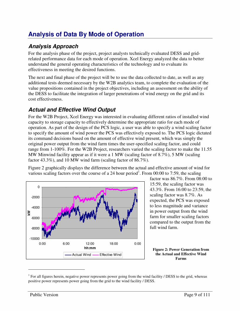
For the W2B Project, Xcel Energy was interested in evaluating different ratios of installed wind capacity to storage capacity to effectively determine the appropriate ratio for each mode of operation. As part of the design of the PCS logic, a user was able to specify a wind scaling factor to specify the amount of wind power the PCS was effectively exposed to. The PCS logic dictated its command decisions based on the amount of effective wind present, which was simply the original power output from the wind farm times the user-specified scaling factor, and could range from 1-100%. For the W2B Project, researchers varied the scaling factor to make the 11.55 MW Minwind facility appear as if it were a 1 MW (scaling factor of 8.7%), 5 MW (scaling factor 43.3%), and 10 MW wind farm (scaling factor of 86.7%).
Figure 2 graphically displays the difference between the actual and effective amount of wind for various scaling factors over the course of a 24 hour period1. From 00:00 to 7:59, the scaling
factor was 86.7%. From 08:00 to 15:59, the scaling factor was 43.3%. From 16:00 to 23:59, the scaling factor was 8.7%. As expected, the PCS was exposed to less magnitude and variance in power output from the wind farm for smaller scaling factors compared to the output from the full wind farm.
Figure 2: Power Generation from
the Actual and Effective Wind
Farms
1 For all figures herein, negative power represents power going from the wind facility / DESS to the grid, whereas positive power represents power going from the grid to the wind facility / DESS.
-10000
-8000
-6000
-4000
-2000
0
0:00 6:00 12:00 18:00 0:00
hh:mm
kW
Actual Wind Effective Wind

Public Version Page 10 of 111
Basic Generation-Storage (GS)
Introduction
One of the value propositions in the W2B Test Plan is to evaluate the ability of large-scale battery storage technology to time shift a variable generation resource. Project analysts used the Basic GS mode to test this proposition by scheduling the battery to discharge during defined on-peak periods and charge during defined off-peak periods at a rate that was proportional and coincident with the power output from the wind farm. Project analysts tested the battery in this mode over a period of six weeks for varying installed wind capacity scenarios, charging options, and discharge profiles.
Theory
One of the objectives in this mode was to gauge the ability of the battery to discharge during the defined on-peak demand periods using one of NGK’s reference duty cycles. For testing purposes, the peak demand hour was based on the hourly averages of 2009 obligation load data for Northern States Power (NSP)2.
Table 2 lists the monthly average peak load hour for NSP, and Figure 3 on the next page shows the monthly average daily load profiles.
Table 2: 2009 Monthly Peak Demand Hours
Month Peak Demand
Hour (CST)
January 18:00
February 18:00
March 09:00
April 10:00
May 11:00
June 13:00
July 14:00
August 14:00
September 13:00
October 18:00
November 17:00
December 17:00
To ensure that the discharge profile remains centered on the peak demand hour, regardless of the initial State of Charge (SOC), the PCS modifies the scheduled discharge duration by delaying the start time and expediting the end time accordingly, depending on the amount of energy available for discharge. The PCS adheres to all the operating constraints placed on the battery by the NGK battery controller.
The Basic GS mode has two variations of charging: wind-only charging and wind-grid charging. For both variations, charging is only allowed during the user-defined charging period, which is specified by a start and end time.
2 Does not account for obligation load Xcel Energy has in balancing authorities outside of NSP.

Public Version Page 11 of 111
Figure 3: 2009 Daily Average NSP Obligation Load Profile
When charging in the wind-only charging option, the DESS begins to charge at a rate that is proportional to the output of the effective wind farm. If the output of the effective wind farm is less than the maximum allowed charge rate, the DESS charges on a one-to-one basis with the amount of wind power available. However, if the output of the effective wind farm exceeds the maximum allowed charge rate, the PCS charges the storage device at its maximum allowed rate (1,100 kW) with the remaining wind power spilling over onto the grid3. Charging terminates either when the end time of the allowed charging window is reached or the battery receives a full charge. A fully-charged battery is determined by the “cut-off voltage”, which is calculated by the NGK battery controller. Because the battery is not permitted to charge by drawing electricity from the grid, the battery may or may not attain a full recharge before its next discharge period.
Charging under the wind-grid option is similar to the wind-only variation except that the battery is capable of charging at its maximum allowed rate, regardless of the output of the effective wind farm. The battery begins to charge at its maximum allowed rate if the battery has still not reached a SOC of 100% before the time specified by the “Grid Allowed Charging Hour” set-point. The storage device continues to charge at its maximum allowed charge rate until it either reaches a full charge state or the allowed charging window expires. Depending on the value entered for the Grid Allowed Charging Hour set-point and the duration of the allowed charging window, the battery may or may not attain a full recharge before its next discharge period.
For both variations of the Basic GS charging options, the NGK battery controller gradually reduces the maximum allowed charge rate for the battery as it approaches a full SOC. NGK implements this charging constraint to reduce the risk of damaging any of the battery modules by
3 Project analysts acknowledge that it is not physically possible to designate electrons from a particular generation facility for a given load. However, this report makes the assumption that when the charging rate is identical to the output of the scaled farm, the battery is charging on wind energy. Conversely, when the charge rate is greater than the output of the scaled farm, the battery is charging on grid energy.
Public Version Page 12 of 111
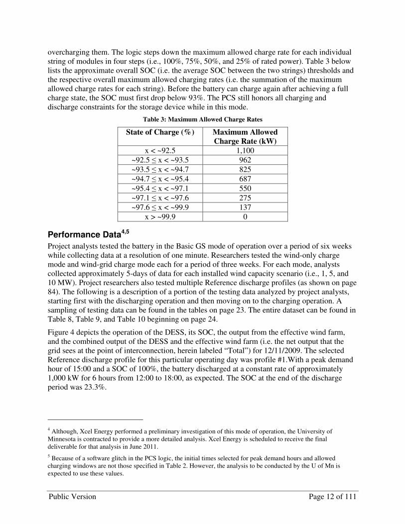
overcharging them. The logic steps down the maximum allowed charge rate for each individual string of modules in four steps (i.e., 100%, 75%, 50%, and 25% of rated power). Table 3 below lists the approximate overall SOC (i.e. the average SOC between the two strings) thresholds and the respective overall maximum allowed charging rates (i.e. the summation of the maximum allowed charge rates for each string). Before the battery can charge again after achieving a full charge state, the SOC must first drop below 93%. The PCS still honors all charging and discharge constraints for the storage device while in this mode.
Table 3: Maximum Allowed Charge Rates
State of Charge (%) Maximum Allowed
Charge Rate (kW)
x < ~92.5 1,100
~92.5 ≤ x < ~93.5 962
~93.5 ≤ x < ~94.7 825
~94.7 ≤ x < ~95.4 687
~95.4 ≤ x < ~97.1 550
~97.1 ≤ x < ~97.6 275
~97.6 ≤ x < ~99.9 137
x > ~99.9 0
Performance Data4,5
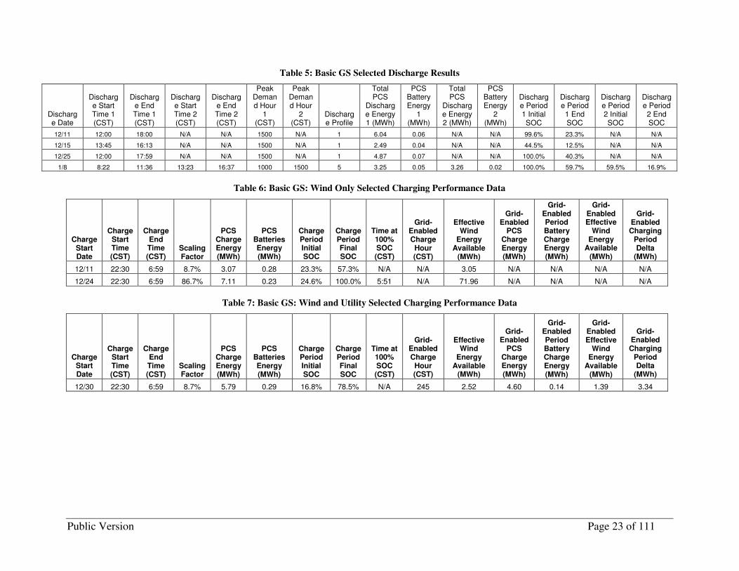
Project analysts tested the battery in the Basic GS mode of operation over a period of six weeks while collecting data at a resolution of one minute. Researchers tested the wind-only charge mode and wind-grid charge mode each for a period of three weeks. For each mode, analysts collected approximately 5-days of data for each installed wind capacity scenario (i.e., 1, 5, and 10 MW). Project researchers also tested multiple Reference discharge profiles (as shown on page 84). The following is a description of a portion of the testing data analyzed by project analysts, starting first with the discharging operation and then moving on to the charging operation. A sampling of testing data can be found in the tables on page 23. The entire dataset can be found in Table 8, Table 9, and Table 10 beginning on page 24.
Figure 4 depicts the operation of the DESS, its SOC, the output from the effective wind farm, and the combined output of the DESS and the effective wind farm (i.e. the net output that the grid sees at the point of interconnection, herein labeled “Total”) for 12/11/2009. The selected Reference discharge profile for this particular operating day was profile #1.With a peak demand hour of 15:00 and a SOC of 100%, the battery discharged at a constant rate of approximately 1,000 kW for 6 hours from 12:00 to 18:00, as expected. The SOC at the end of the discharge period was 23.3%.
4 Although, Xcel Energy performed a preliminary investigation of this mode of operation, the University of Minnesota is contracted to provide a more detailed analysis. Xcel Energy is scheduled to receive the final deliverable for that analysis in June 2011.
5 Because of a software glitch in the PCS logic, the initial times selected for peak demand hours and allowed charging windows are not those specified in Table 2. However, the analysis to be conducted by the U of Mn is expected to use these values.

Public Version Page 13 of 111
-2000
-1500
-1000
-500
0
500
1000
1500
0:00 3:00 6:00 9:00 12:00 15:00 18:00 21:00 0:00
hh:mm
kW
0%
20%
40%
60%
80%
100%
SO
C
DESS (kW) Effective Wind (kW) Total (kW) SOC (%)
Figure 4: Basic GS, Discharge Profile #1, Fully Charged (12/11)
Figure 5 displays system performance data for discharge profile #1 for a partially-charged battery. At the completion of the previous charging session (partly shown in the figure) the SOC of the battery was 44.5%, which was not capable of providing the energy required by the scheduled profile. Therefore, the PCS delayed the start of the discharge by 1 hour and 45 minutes and started to discharge at 1,000 kW at 13:45. After discharging for approximately 2.5 hours at a constant 1,000 kW, the DESS stopped discharging at 16:14. By delaying the discharge start time and expediting the discharge end time, the DESS was still able to discharge during the defined peak demand period. The SOC at the end of the discharge period was 12.4%.
-2000
-1500
-1000
-500
0
500
1000
1500
0:00 3:00 6:00 9:00 12:00 15:00 18:00 21:00 0:00
hh:mm
kW
0%
20%
40%
60%
80%
100%S
OC
DESS (kW) Effective Wind (kW) Total (kW) SOC (%)
Figure 5: Basic GS, Discharge Profile #1, Partially Charged (12/15)

Public Version Page 14 of 111
Researchers also tested the Reference discharge profile #4 during the Basic GS testing period. Figure 6 displays the data for a sample discharge period on 1/8/2010. The user specified peak demand hours of 10:00 and 15:00 for the individual discharge periods for this profile. As expected, with a fully-charged battery, the PCS discharged the battery for 3.2 hours at a constant rate of approximately 1,000 kW for each scheduled discharge period. The DESS discharged 3.25 MWh in the first discharge period and 3.26 MWh in the second. The SOC at the completion of the second discharge period was 16.9%.
-6000
-5000
-4000
-3000
-2000
-1000
0
1000
2000
0:00 3:00 6:00 9:00 12:00 15:00 18:00 21:00 0:00
hh:mm
kW
0%
20%
40%
60%
80%
100%
SO
C
DESS (kW) Effective Wind (kW) Total (kW) SOC (%)
Figure 6: Basic GS Discharge Profile #4, Fully-Charged (1/8)
The combined output of the DESS and MWD facility cannot exceed 12 MW at the point of grid interconnection due to contractual reasons between MWD and MISO. Thus, when the output of the wind farm is above 11 MW while the DESS is discharging, the PCS curtails the output of the battery accordingly to not exceed this threshold. Figure 7 is an example of an instance when this occurs during the Basic GS mode of operation for discharge profile #1. As shown in the figure, the wind farm was producing power at or near its rated capacity coincident to the scheduled discharge period for the DESS. As a result, the PCS limited the battery discharge rate between 275-1,000 kW throughout the discharge period. Thus, the storage device was only able to discharge 4.87 MWh of energy during the discharge period rather than the expected 6 MWh. The SOC at the end of the discharge period was 40%.

Public Version Page 15 of 111
-12000
-10000
-8000
-6000
-4000
-2000
0
2000
0:00 6:00 12:00 18:00 0:00
hh:mm
kW
0%
20%
40%
60%
80%
100%
SO
C
DESS (kW) Actual Wind (kW) SOC (%)
Figure 7: Basic GS, Discharge Profile #1, Actual Wind Farm Output (12/25)
All of the Reference discharge profiles are scheduled to have a final SOC at or near 10% upon completing its complete discharge schedule. However, as illustrated by the figures and Table 8, the DESS is currently capable of discharging more than the scheduled energy amount. Because the performance of the NaS modules gradually degrades over time, NGK conservatively estimated the discharge duration times using end-of-life conditions.
For each discharge period, project analysts normalized the amount of energy discharged with the percent change in SOC. For example, on 12/11/2009 the DESS discharged 6.04 MWh as it went from an initial SOC of 99.6% to a final SOC 23.3%. Thus, the normalized discharged energy for this particular day was 7.9 MWh/%6. Figure 8 and Figure 9 display this calculated value for each discharge period during the Basic GS testing period for profiles #1 and #5, respectively.
As illustrated in both figures, there is considerable variability in the results from one day to the next. Furthermore, Figure 9 displays additional interesting behavior that was not originally accounted for by any of the project participants. In the figure, the “I” data series represents the first discharge period for profile #4, whereas the “II” data series represents the second. From the figure, the normalized discharge energy is dependent on the SOC range it spans while discharging. By definition, the II data series is always over a lower SOC range than the I data series since it is the second discharge period. Therefore, it appears that the battery delivers more discharge energy per percent change in SOC for higher states of charge than lower states of charge. After discussions with NGK, project analysts attribute the variability in these results to inaccuracies in current measurements by the NGK battery controller as well as the manner in which NGK calculates SOC (i.e. using Ah discharged rather than kWh discharged). However, further testing is required to prove or disprove this statement.
6 6.04÷(99.6%-23.3%)

Public Version Page 16 of 111
7.6
7.7
7.8
7.9
8.0
8.1
8.2
0 1 2 3 4 5 6 7 8 9 10 11 12 13 14 15 16 17 18
Discharge Trial Period
MW
h_d
/ S
OC
_D
elt
a
Figure 8: Normalized Discharge Energy Based on Change in State of Charge (Profile #1)
7.5
7.6
7.7
7.8
7.9
8.0
8.1
8.2
8.3
8.4
8.5
0 1 2 3 4 5 6 7 8 9 10 11 12 13 14 15 16 17 18 19 20 21
Discharge Trial Period
MW
h_
d /
SO
C_
de
lta
I II
Figure 9: Normalized Discharge Energy Based on Change in State of Charge (Profile #4)

Public Version Page 17 of 111
In general, the PCS performed as expected during the discharging operation of the Basic GS mode of operation, but project analysts did uncover some unexpected operation. For any partial discharge period, project analysts expected the final SOC to be 10% (the minimum allowed SOC value). However, as shown in Table 8 this was not always the case. According to S&C, the final SOC value did not exactly equal 10 % due to (a) higher than expected efficiencies in the PCS7 and (b) NGK calculating SOC based on Ahs rather than kWhs. Furthermore, for profile #4, the PCS did not accurately calculate the start and end times for partial discharge periods, even after accounting for the high PCS efficiency and any inaccuracies in the SOC measurement. Notified by Xcel Energy of the error, S&C will account for it in the updated software to be installed by Q3 2010.
Figure 10 displays system operation data while the DESS is charging under the wind-only mode during the evening of 12/24/2009 and 12/25/2009. The capacity of the effective wind farm for this charging period was 10 MW, and the allowed charging period was from 22:30 to 07:00. At 22:30, with a SOC of 24.6%, the battery began to charge at its maximum allowed charge rate and continued to do so throughout the entire charging period because the output of the effective wind farm exceeded 1,100 kW. As a result, the only difference between the Total and Effective Wind Farm data series was an offset of 1,100 kW. At 04:27 at a SOC of 93.6%, the PCS began to reduce the maximum allowed charging rate of the battery according to the step-down charging algorithm controlled by the NGK battery controller. At 05:51, the battery achieved a SOC of 100% and remained idle for the remaining portion of the allowed charging window. During the charging period, the DESS consumed 7.11 MWh of energy while the effective wind farm generated nearly 72 MWh.
-10000
-8000
-6000
-4000
-2000
0
2000
12:00 15:00 18:00 21:00 0:00 3:00 6:00 9:00 12:00
hh:mm
kW
0%
20%
40%
60%
80%
100%
SO
C
DESS (kW) Effective Wind (kW) Total (kW)l SOC (%)
Figure 10: Basic GS: Wind Only Charging Operation (12/24-12/25)
7 For discharging, S&C assumed a constant efficiency of 95% for the PCS; however, it appears that the PCS is ~96-97% efficient.
Public Version Page 18 of 111
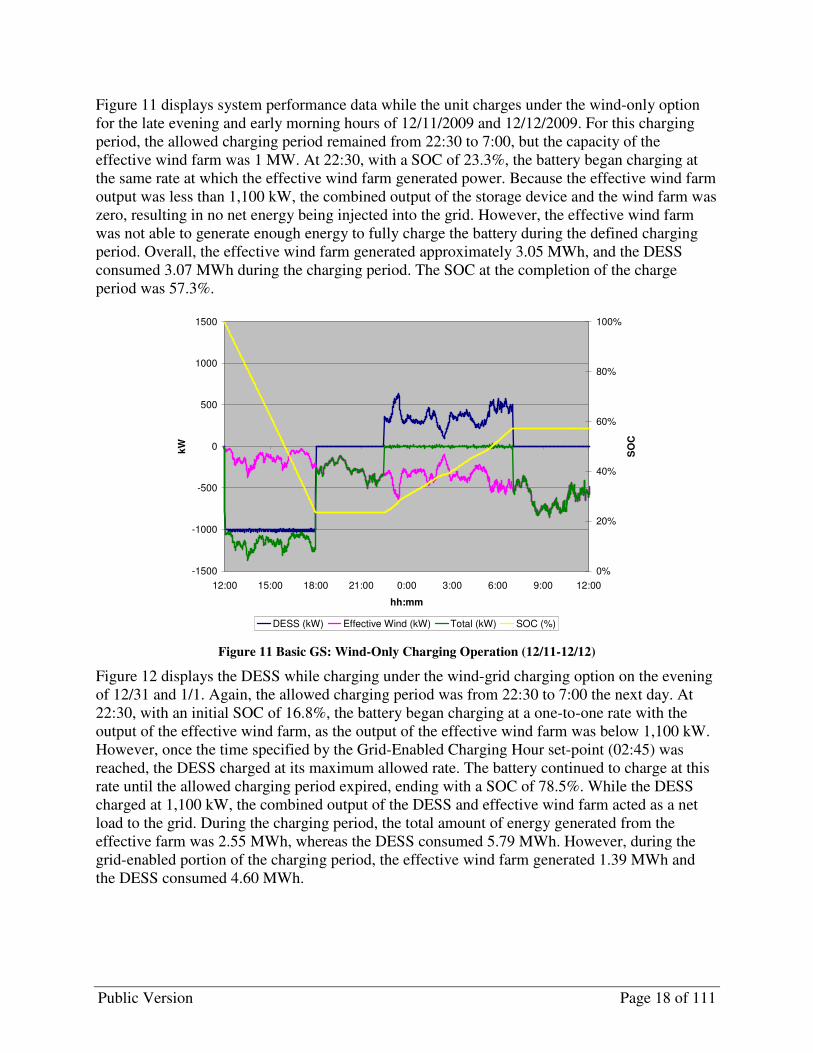
Figure 11 displays system performance data while the unit charges under the wind-only option for the late evening and early morning hours of 12/11/2009 and 12/12/2009. For this charging period, the allowed charging period remained from 22:30 to 7:00, but the capacity of the effective wind farm was 1 MW. At 22:30, with a SOC of 23.3%, the battery began charging at the same rate at which the effective wind farm generated power. Because the effective wind farm output was less than 1,100 kW, the combined output of the storage device and the wind farm was zero, resulting in no net energy being injected into the grid. However, the effective wind farm was not able to generate enough energy to fully charge the battery during the defined charging period. Overall, the effective wind farm generated approximately 3.05 MWh, and the DESS consumed 3.07 MWh during the charging period. The SOC at the completion of the charge period was 57.3%.
-1500
-1000
-500
0
500
1000
1500
12:00 15:00 18:00 21:00 0:00 3:00 6:00 9:00 12:00
hh:mm
kW
0%
20%
40%
60%
80%
100%
SO
CDESS (kW) Effective Wind (kW) Total (kW) SOC (%)
Figure 11 Basic GS: Wind-Only Charging Operation (12/11-12/12)
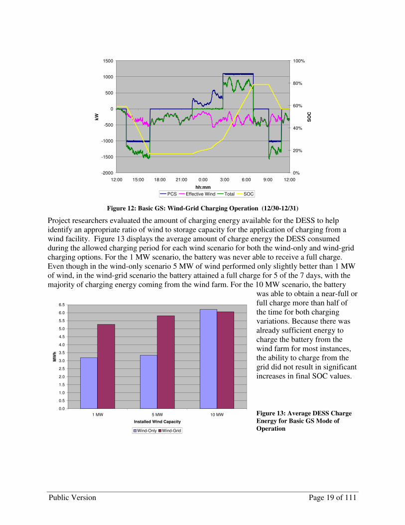
Figure 12 displays the DESS while charging under the wind-grid charging option on the evening of 12/31 and 1/1. Again, the allowed charging period was from 22:30 to 7:00 the next day. At 22:30, with an initial SOC of 16.8%, the battery began charging at a one-to-one rate with the output of the effective wind farm, as the output of the effective wind farm was below 1,100 kW. However, once the time specified by the Grid-Enabled Charging Hour set-point (02:45) was reached, the DESS charged at its maximum allowed rate. The battery continued to charge at this rate until the allowed charging period expired, ending with a SOC of 78.5%. While the DESS charged at 1,100 kW, the combined output of the DESS and effective wind farm acted as a net load to the grid. During the charging period, the total amount of energy generated from the effective farm was 2.55 MWh, whereas the DESS consumed 5.79 MWh. However, during the grid-enabled portion of the charging period, the effective wind farm generated 1.39 MWh and the DESS consumed 4.60 MWh.
Public Version Page 19 of 111
0.0
0.5
1.0
1.5
2.0
2.5
3.0
3.5
4.0
4.5
5.0
5.5
6.0
6.5
1 MW 5 MW 10 MW
Installed Wind Capacity
MW
h
Wind-Only Wind-Grid
-2000
-1500
-1000
-500
0
500
1000
1500
12:00 15:00 18:00 21:00 0:00 3:00 6:00 9:00 12:00
hh:mm
kW
0%
20%
40%
60%
80%
100%
SO
C
PCS Effective Wind Total SOC
Figure 12: Basic GS: Wind-Grid Charging Operation (12/30-12/31)
Project researchers evaluated the amount of charging energy available for the DESS to help identify an appropriate ratio of wind to storage capacity for the application of charging from a wind facility. Figure 13 displays the average amount of charge energy the DESS consumed during the allowed charging period for each wind scenario for both the wind-only and wind-grid charging options. For the 1 MW scenario, the battery was never able to receive a full charge. Even though in the wind-only scenario 5 MW of wind performed only slightly better than 1 MW of wind, in the wind-grid scenario the battery attained a full charge for 5 of the 7 days, with the majority of charging energy coming from the wind farm. For the 10 MW scenario, the battery
was able to obtain a near-full or full charge more than half of the time for both charging variations. Because there was already sufficient energy to charge the battery from the wind farm for most instances, the ability to charge from the grid did not result in significant increases in final SOC values.
Figure 13: Average DESS Charge
Energy for Basic GS Mode of
Operation

Public Version Page 20 of 111
Similar to the discharge operation, project analysts normalized the amount of charge energy with the percent change in SOC for each charging period. Figure 14 displays the calculated values for each charging period for both charging modes. Similar to the discharging data, the charging data exhibits variability in the results from one day to the next but does so at a slightly less degree of variance. Again, project analysts assume the variability in these results to the aforementioned sources of error but further testing is required to evaluate the validity of this assumption.
Figure 14: Normalized Charge Energy
Based on Change in State of Charge
As mentioned before, the NGK battery controller implements a charging constraint on the battery whenever it approaches a full state of charge. To gauge the overall impact on system performance of this constraint, project analysts tracked at what overall state of charge the overall maximum allowed charge rate was reduced for each charging session that attained a sufficient amount of charging energy. Figure 15 displays the corresponding SOC values for each maximum allowed charge rate listed in Table 3 on page 11. Each maximum allowed charge rating has a significant amount of variability in the SOC values. Project analysts suspect that slight
discrepancies in SOC values between the two strings as well as any inaccuracies in NGK’s SOC calculations were the primary sources of variability in the results. The maximum allowed charge rate returned to 1,100 kW once the SOC dropped below 92-93% as expected.
Figure 15: Maximum Allowed
Charge Rate as Function of SOC
8.9
9.0
9.1
9.2
9.3
9.4
9.5
9.6
9.7
9.8
0 5 10 15 20 25 30 35 40
Charge Trial Period
MW
h_C
/ S
OC
Delt
a
90.0%
92.5%
95.0%
97.5%
100.0%
0 100 200 300 400 500 600 700 800 900 1000
Maximum Allowed Charge Rate (kW)
SO
C

Public Version Page 21 of 111
In addition to tracking the energy in and out of the DESS during the charging and discharging periods, project analysts also tracked the operation of the auxiliary load throughout the testing period. Figure 16 displays the operation of the DESS and the power draw of the auxiliary loads for 12/11. As illustrated, the module heaters operated at a variable rate depending on battery operation and ambient weather conditions. For the majority of discharge periods, the auxiliary energy requirements of the DESS were minimal8. For this particular discharge period, the total energy requirement of the auxiliary load was 0.06 MWh and .28 MWh for the charging period. These results were similar for the other days analyzed. During the testing of the Basic GS mode of operation, the overall efficiency of the DESS, including the auxiliary energy requirements of the device, averaged 73.7%.
Figure 16: DESS and Auxiliary
Power Output (12/11)
Conclusions
Overall, the DESS performed as expected for the majority of scenarios tested in the Basic GS mode of operation. When discharging according to profile #1, the PCS operated at the appropriate times for both full and partial discharge periods. For profile #4, the PCS operated as expected when there was sufficient energy available for a full discharge, but for a partial discharge period S&C must modify the PCS software. For the wind-only charging mode, the amount of energy consumed by the DESS while charging was near or equal to the amount of energy generated by the effective wind farm during the charging session. In the wind-grid charging mode, the PCS correctly charged at its maximum allowed rate during the appropriate times.
For an allowed charging window of 8.5 hours, the 1 MW wind scenario is not sufficient to fully charge the battery in a single charging session. On the contrary, the 10 MW wind scenario provides sufficient energy to charge the battery with a large amount of excess wind energy left over. For the 5 MW scenario, there was a large degree of variability in the results, thus project researchers recommend additional tests, especially for the 5 MW scenario. This will enable project researchers to better understand the appropriate amount of wind energy needed for the
8 The minimum power draw of the auxiliary load of the PCS is 6 kW due to the power requirements of the power electronics.
-1500
-1000
-500
0
500
1000
1500
0:00 3:00 6:00 9:00 12:00 15:00 18:00 21:00 0:00
hh:mm
DE
SS
0
10
20
30
40
50
60
70
80
90
100
Au
xilia
ry
DESS (kW) Auxiliary (kW)

Public Version Page 22 of 111
time-shifting application. According to the data collected for this particular testing period, results show that the optimal ratio of wind farm capacity to DESS capacity for time shifting applications is greater than 5:1, but less than 10:1.
Table 4 lists the system performance data of interest for each testing variation conducted in the Basic GS mode of operation. For the Basic GS testing period, the average mileage of the DESS was 22,170 kW/day. Moreover, the battery never exceeded more than one discharge cycle in any given day, averaging 0.77 cycles throughout the tests. The average daily auxiliary energy requirement was 720 kWh/day. The overall efficiency of the DESS with and without the auxiliary energy requirements averaged 73.7% and 85.1%, respectively.
Table 4: Basic GS System Performance Data Statistics Summary
Mode
Installed
Wind
Capacity
(MW)
Discharge
Profile
Mileage9
(kW/day)
Daily
Discharge
Cycle
Usage10
Aux Energy
Requirement
(kWh/day) η111
η212
Wind-Only 1 1 17,501 0.69 876 69.4% 87.1%
Wind-Only 5 1 21,726 0.61 870 70.0% 85.6%
Wind-Only 10 1 23,258 0.93 616 78.4% 85.2%
Wind-Grid 1 5 17,414 0.77 734 72.8% 84.5%
Wind-Grid 5 5 31,987 0.80 674 75.4% 84.5%
Wind-Grid 10 5 21,134 0.83 550 76.4% 83.6%
9 Mileage is the metric used to gauge the “stress” of the duty profile imposed on the battery. It is the cumulative sum of the absolute value of the change in PCS power settings from one time step to the next, thereby giving an indication of the linear length of the duty profile.
10 NGK has multiple daily discharge cycles, or profiles, which vary in shape, duration and number of discharge periods. These are further described in the NaS Battery Durability section of this document.
11 η1, also known as “eta_1” measures the DESS Overall System Efficiency, including auxiliary loads.
12 η2, also known as “eta_2” measures the DESS Overall System Efficiency, excluding auxiliary loads.
Public Version Page 23 of 111
Table 5: Basic GS Selected Discharge Results
Discharge Date
Discharge Start Time 1 (CST)
Discharge End Time 1 (CST)
Discharge Start Time 2 (CST)
Discharge End Time 2 (CST)
Peak Demand Hour
1 (CST)
Peak Demand Hour
2 (CST)
Discharge Profile
Total PCS
Discharge Energy 1 (MWh)
PCS Battery Energy
1 (MWh)
Total PCS
Discharge Energy 2 (MWh)
PCS Battery Energy
2 (MWh)
Discharge Period 1 Initial SOC
Discharge Period 1 End SOC
Discharge Period 2 Initial SOC
Discharge Period 2 End SOC
12/11 12:00 18:00 N/A N/A 1500 N/A 1 6.04 0.06 N/A N/A 99.6% 23.3% N/A N/A
12/15 13:45 16:13 N/A N/A 1500 N/A 1 2.49 0.04 N/A N/A 44.5% 12.5% N/A N/A
12/25 12:00 17:59 N/A N/A 1500 N/A 1 4.87 0.07 N/A N/A 100.0% 40.3% N/A N/A
1/8 8:22 11:36 13:23 16:37 1000 1500 5 3.25 0.05 3.26 0.02 100.0% 59.7% 59.5% 16.9%
Table 6: Basic GS: Wind Only Selected Charging Performance Data
Charge Start Date
Charge Start Time (CST)
Charge End Time (CST)
Scaling Factor
PCS Charge Energy (MWh)
PCS Batteries Energy (MWh)
Charge Period Initial SOC
Charge Period Final SOC
Time at 100% SOC (CST)
Grid-Enabled Charge Hour (CST)
Effective Wind
Energy Available
(MWh)
Grid-Enabled
PCS Charge Energy (MWh)
Grid-Enabled Period Battery Charge Energy (MWh)
Grid-Enabled Effective
Wind Energy
Available (MWh)
Grid-Enabled Charging
Period Delta
(MWh)
12/11 22:30 6:59 8.7% 3.07 0.28 23.3% 57.3% N/A N/A 3.05 N/A N/A N/A N/A
12/24 22:30 6:59 86.7% 7.11 0.23 24.6% 100.0% 5:51 N/A 71.96 N/A N/A N/A N/A
Table 7: Basic GS: Wind and Utility Selected Charging Performance Data
Charge Start Date
Charge Start Time (CST)
Charge End Time (CST)
Scaling Factor
PCS Charge Energy (MWh)
PCS Batteries Energy (MWh)
Charge Period Initial SOC
Charge Period Final SOC
Time at 100% SOC (CST)
Grid-Enabled Charge Hour (CST)
Effective Wind
Energy Available
(MWh)
Grid-Enabled
PCS Charge Energy (MWh)
Grid-Enabled Period Battery Charge Energy (MWh)
Grid-Enabled Effective
Wind Energy
Available (MWh)
Grid-Enabled Charging
Period Delta
(MWh)
12/30 22:30 6:59 8.7% 5.79 0.29 16.8% 78.5% N/A 245 2.52 4.60 0.14 1.39 3.34

Public Version Page 24 of 111
Table 8: Basic GS All Discharge Results
Discharge Date
Discharge Start
Time 1 (CST)
Discharge End
Time 1 (CST)
Discharge Start
Time 2 (CST)
Discharge End Time 2 (CST)
Peak Demand Hour 1 (CST)
Peak Demand Hour 2 (CST)
Discharge Profile
Total PCS Discharge Energy 1
(MWh)
PCS Batteries Energy 1
(MWh)
Total PCS Discharge Energy 2
(MWh)
PCS Batteries Energy 2
(MWh)
Discharge Period 1
Initial SOC
Discharge Period 1 End SOC
Discharge Period 2
Initial SOC
Discharge Period 2 End SOC
12/11 12:00 18:00 N/A N/A 1500 N/A 1 6.04 0.06 N/A N/A 99.6% 23.3% N/A N/A
12/12 13:18 16:41 N/A N/A 1500 N/A 1 3.41 0.04 N/A N/A 57.1% 12.9% N/A N/A
12/13 13:20 16:39 N/A N/A 1500 N/A 1 3.35 0.05 N/A N/A 56.3% 13.3% N/A N/A
12/14 13:44 16:16 N/A N/A 1500 N/A 1 2.56 0.04 N/A N/A 45.3% 12.6% N/A N/A
12/15 13:45 16:13 N/A N/A 1500 N/A 1 2.49 0.04 N/A N/A 44.5% 12.5% N/A N/A
12/16 12:00 N/A N/A 1500 N/A 1 6.02 0.06 N/A N/A 97.5% 21.5% N/A N/A
12/17 13:14 16:45 N/A N/A 1500 N/A 1 3.54 0.05 N/A N/A 59.1% 13.3% N/A N/A
12/18 14:16 15:43 N/A N/A 1500 N/A 1 1.46 0.03 N/A N/A 30.4% 11.5% N/A N/A
12/19 12:55 17:05 N/A N/A 1500 N/A 1 4.20 0.04 N/A N/A 68.1% 14.2% N/A N/A
12/20 14:11 15:47 N/A N/A 1500 N/A 1 1.61 0.03 N/A N/A 32.5% 11.6% N/A N/A
12/22 12:00 17:59 N/A N/A 1500 N/A 1 6.03 0.07 N/A N/A 99.9% 24.1% N/A N/A
12/23 11:59 17:59 N/A N/A 1500 N/A 1 6.03 0.07 N/A N/A 100.0% 23.8% N/A N/A
12/24 12:00 17:59 N/A N/A 1500 N/A 1 6.02 0.07 N/A N/A 100.0% 24.7% N/A N/A
12/25 12:00 17:59 N/A N/A 1500 N/A 1 4.87 0.07 N/A N/A 100.0% 40.3% N/A N/A
12/26 12:00 17:59 N/A N/A 1500 N/A 1 6.03 0.06 N/A N/A 100.0% 24.1% N/A N/A
12/27 12:00 17:59 N/A N/A 1500 N/A 1 6.04 0.07 N/A N/A 99.8% 23.7% N/A N/A
12/28 12:00 17:59 N/A N/A 1500 N/A 1 6.01 0.08 N/A N/A 100.0% 24.4% N/A N/A
12/30 N/A N/A 13:22 16:36 N/A 1500 5 N/A N/A 3.26 0.02 N/A N/A 59.5% 16.9%
12/31 9:07 10:51 14:07 15:51 1000 1500 5 1.75 0.04 1.75 0.05 78.8% 57.2% 57.1% 34.6%
1/1 8:30 11:30 13:29 16:30 1000 1500 5 3.02 0.05 3.03 0.03 96.5% 59.3% 59.2% 19.9%
1/2 9:13 10:46 14:13 15:46 1000 1500 5 1.56 0.03 1.56 0.04 76.0% 56.8% 56.6% 36.8%
1/3 8:36 11:23 13:36 16:24 1000 1500 5 2.79 0.04 2.82 0.03 93.6% 58.9% 58.6% 22.0%
1/4 9:25 10:34 14:25 15:34 1000 1500 5 1.16 0.03 1.17 0.03 70.7% 56.3% 56.0% 41.3%
1/5 8:42 11:16 N/A N/A 1000 N/A 5 2.58 0.04 N/A N/A 90.3% 58.2% N/A N/A
1/6 N/A N/A 13:42 16:17 N/A 1500 5 N/A N/A 2.59 0.04 N/A N/A 77.1% 44.4%
1/7 8:23 11:36 13:22 16:36 1000 1500 5 1.95 0.08 2.03 0.09 100.0% 76.7% 76.6% 52.2%
1/8 8:22 11:36 13:23 16:37 1000 1500 5 3.25 0.05 3.26 0.02 100.0% 59.7% 59.5% 16.9%

Public Version Page 25 of 111
Discharge Date
Discharge Start
Time 1 (CST)
Discharge End
Time 1 (CST)
Discharge Start
Time 2 (CST)
Discharge End Time 2 (CST)
Peak Demand Hour 1 (CST)
Peak Demand Hour 2 (CST)
Discharge Profile
Total PCS Discharge Energy 1
(MWh)
PCS Batteries Energy 1
(MWh)
Total PCS Discharge Energy 2
(MWh)
PCS Batteries Energy 2
(MWh)
Discharge Period 1
Initial SOC
Discharge Period 1 End SOC
Discharge Period 2
Initial SOC
Discharge Period 2 End SOC
1/9 9:36 10:23 14:36 15:23 1000 1500 5 0.79 0.03 0.79 0.03 65.5% 55.8% 55.5% 45.5%
1/10 8:23 11:37 13:23 16:37 1000 1500 5 3.24 0.04 3.27 0.02 99.9% 59.4% 59.4% 16.6%
1/11 8:23 11:36 13:22 16:36 1000 1500 5 3.23 0.05 3.26 0.02 99.9% 59.7% 59.7% 17.1%
1/12 8:50 11:09 13:50 16:09 1000 1500 5 2.33 0.04 2.33 0.04 86.8% 58.1% 57.7% 27.7%
1/13 8:23 11:36 13:23 16:36 1000 1500 5 3.23 0.04 3.25 0.02 99.7% 59.9% 59.5% 17.3%
1/14 8:23 11:36 13:22 16:36 1000 1500 5 3.22 0.05 3.25 0.02 99.7% 59.7% 59.6% 17.1%
1/15 9:36 10:24 14:36 15:23 1000 1500 5 0.80 0.03 0.79 0.03 65.7% 55.7% 55.5% 45.6%
1/16 8:23 11:37 13:23 16:37 1000 1500 5 3.24 0.03 3.26 0.02 99.9% 59.7% 59.6% 17.0%
1/17 9:29 10:30 14:29 15:30 1000 1500 5 1.03 0.04 1.03 0.04 68.7% 56.1% 55.9% 42.9%
1/18 8:23 11:37 13:23 16:36 1000 1500 5 3.24 0.04 3.25 0.02 99.9% 59.7% 59.5% 17.2%
1/19 8:49 11:09 13:50 16:09 1000 1500 5 2.35 0.04 2.35 0.04 87.0% 57.8% 57.6% 27.3%
1/20 8:23 11:36 13:23 16:37 1000 1500 5 3.24 0.04 3.26 0.02 100.0% 59.9% 59.7% 17.1%
1/21 8:37 11:22 N/A N/A 1000 N/A 5 2.76 0.04 N/A N/A 92.8% 58.4% N/A N/A
Table 9: Basic GS: Wind Only All Charging Performance Data
Charge Start Date
Charge Start Time (CST)
Charge End Time (CST)
Scaling Factor
PCS Charge Energy (MWh)
PCS Batteries Energy (MWh)
Charge Period Initial SOC
Charge Period Final SOC
Time at 100% SOC (CST)
Grid-Enabled Charge Hour (CST)
Effective Wind
Energy Available
(MWh)
Grid-Enabled
PCS Charge Energy (MWh)
Grid-Enabled Period Battery Charge Energy (MWh)
Grid-Enabled Effective
Wind Energy
Available (MWh)
Grid-Enabled Charging
Period Delta
(MWh)
12/11 22:30 6:59 8.7% 3.07 0.28 23.3% 57.3% N/A N/A 3.05 N/A N/A N/A N/A
12/12 22:30 6:59 8.7% 3.94 0.44 12.8% 56.3% N/A N/A 3.92 N/A N/A N/A N/A
12/13 22:30 6:59 8.7% 2.91 0.51 13.2% 45.5% N/A N/A 2.87 N/A N/A N/A N/A
12/14 22:30 6:59 8.7% 2.86 0.52 12.6% 44.5% N/A N/A 2.87 N/A N/A N/A N/A
12/15 22:30 6:59 43.3% 8.03 0.26 12.5% 97.5% N/A N/A 16.02 N/A N/A N/A N/A
12/16 22:30 6:59 43.3% 3.42 0.27 21.6% 59.2% N/A N/A 3.46 N/A N/A N/A N/A
12/17 22:30 6:59 43.3% 1.62 0.39 13.1% 30.6% N/A N/A 1.73 N/A N/A N/A N/A

Public Version Page 26 of 111
Charge Start Date
Charge Start Time (CST)
Charge End Time (CST)
Scaling Factor
PCS Charge Energy (MWh)
PCS Batteries Energy (MWh)
Charge Period Initial SOC
Charge Period Final SOC
Time at 100% SOC (CST)
Grid-Enabled Charge Hour (CST)
Effective Wind
Energy Available
(MWh)
Grid-Enabled
PCS Charge Energy (MWh)
Grid-Enabled Period Battery Charge Energy (MWh)
Grid-Enabled Effective
Wind Energy
Available (MWh)
Grid-Enabled Charging
Period Delta
(MWh)
12/18 22:30 6:59 43.3% 5.23 0.47 11.4% 68.2% N/A N/A 5.63 N/A N/A N/A N/A
12/19 22:30 6:59 43.3% 1.69 0.34 14.1% 32.6% N/A N/A 1.73 N/A N/A N/A N/A
12/20 22:30 6:59 43.3% 0.06 0.46 11.5% 12.1% N/A N/A 0.00 N/A N/A N/A N/A
12/22 22:30 6:59 86.7% 7.21 0.16 24.1% 100.0% 5:52 N/A 23.41 N/A N/A N/A N/A
12/23 22:30 6:59 86.7% 7.12 0.22 23.8% 100.0% 6:48 N/A 18.21 N/A N/A N/A N/A
12/24 22:30 6:59 86.7% 7.11 0.23 24.6% 100.0% 5:51 N/A 71.96 N/A N/A N/A N/A
12/25 22:30 6:59 86.7% 5.63 0.34 40.2% 100.0% 6:58 N/A 27.74 N/A N/A N/A N/A
12/26 22:30 6:59 86.7% 7.15 0.19 24.1% 99.8% N/A N/A 33.81 N/A N/A N/A N/A
12/27 22:30 6:59 86.7% 7.17 0.19 23.7% 100.0% 5:55 N/A 51.15 N/A N/A N/A N/A
12/28 22:30 6:59 86.7% 1.93 0.31 24.2% 44.6% N/A N/A 3.47 N/A N/A N/A N/A
Table 10: Basic GS: Wind and Utility All Charging Performance Data
Charge Start Date
Charge Start Time (CST)
Charge End Time (CST)
Scaling Factor
PCS Charge Energy (MWh)
PCS Batteries Energy (MWh)
Charge Period Initial SOC
Charge Period Final SOC
Time at 100% SOC (CST)
Grid-Enabled Charge Hour (CST)
Effective Wind
Energy Available
(MWh)
Grid-Enabled
PCS Charge Energy (MWh)
Grid-Enabled Period Battery Charge Energy (MWh)
Grid-Enabled Effective
Wind Energy
Available (MWh)
Grid-Enabled Charging
Period Delta
(MWh)
12/30 22:30 6:59 8.7% 5.79 0.29 16.8% 78.5% N/A 245 2.52 4.60 0.14 1.39 3.34
12/31 22:30 6:59 8.7% 5.80 0.41 34.5% 96.6% N/A 245 3.22 4.29 0.15 1.65 2.79
1/1 22:30 6:59 8.7% 5.33 0.36 19.7% 76.0% N/A 245 1.13 4.61 0.19 0.44 4.37
1/2 22:31 6:59 8.7% 5.38 0.37 36.7% 93.7% N/A 245 0.96 4.54 0.13 0.17 4.50
1/3 22:30 6:59 8.7% 4.62 0.32 21.9% 70.6% N/A 245 0.00 4.61 0.15 0.00 4.75
1/4 22:30 6:59 8.7% 4.66 0.37 41.1% 90.3% N/A 245 0.00 4.62 0.14 0.00 4.76
1/6 22:30 6:59 43.3% 5.23 0.42 44.4% 100.0% 3:56 245 40.70 0.61 0.23 20.78 -19.95

Public Version Page 27 of 111
Charge Start Date
Charge Start Time (CST)
Charge End Time (CST)
Scaling Factor
PCS Charge Energy (MWh)
PCS Batteries Energy (MWh)
Charge Period Initial SOC
Charge Period Final SOC
Time at 100% SOC (CST)
Grid-Enabled Charge Hour (CST)
Effective Wind
Energy Available
(MWh)
Grid-Enabled
PCS Charge Energy (MWh)
Grid-Enabled Period Battery Charge Energy (MWh)
Grid-Enabled Effective
Wind Energy
Available (MWh)
Grid-Enabled Charging
Period Delta
(MWh)
1/7 22:30 6:59 43.3% 4.53 0.41 52.2% 100.0% 3:06 245 35.94 0.09 0.26 15.16 -14.80
1/8 22:30 6:59 43.3% 4.62 0.32 16.9% 65.6% N/A 245 0.00 4.61 0.15 0.00 4.76
1/9 22:30 6:59 43.3% 5.09 0.34 45.4% 100.0% 4:14 245 32.48 0.52 0.22 14.29 -13.55
1/10 22:30 6:59 43.3% 7.87 0.20 16.6% 100.0% 6:44 245 23.38 3.24 0.10 10.83 -7.49
1/11 22:30 6:59 43.3% 6.59 0.24 17.0% 86.8% N/A 245 12.12 4.61 0.09 9.96 -5.25
1/12 22:31 6:59 43.3% 6.72 0.25 27.7% 100.0% 6:02 245 8.66 2.38 0.14 3.46 -0.95
1/13 22:30 6:59 86.6% 7.85 0.16 17.3% 100.0% 6:45 245 31.18 3.28 0.08 14.72 -11.36
1/14 22:30 7:00 86.6% 4.63 0.26 16.9% 65.7% N/A 245 0.00 4.61 0.12 0.00 4.73
1/15 22:30 6:59 86.6% 5.10 0.34 45.6% 100.0% 4:18 245 23.38 0.56 0.22 11.26 -10.48
1/16 22:30 6:59 86.6% 4.92 0.23 17.0% 68.6% N/A 245 0.00 4.61 0.12 0.00 4.73
1/17 22:30 6:59 86.6% 5.39 0.33 42.8% 100.0% 6:17 245 2.60 2.76 0.15 0.00 2.91
1/18 22:30 6:59 86.6% 6.58 0.20 17.1% 87.0% N/A 245 2.60 4.61 0.08 0.00 4.70
1/19 22:30 6:59 86.6% 6.88 0.26 27.2% 100.0% 5:53 245 32.04 2.26 0.14 18.19 -15.78
1/20 22:30 6:59 86.6% 7.16 0.18 17.1% 92.8% N/A 245 5.20 4.61 0.09 0.87 3.83

Public Version Page 28 of 111
Economic Dispatch (ED)
Introduction
Another value proposition in the W2B Test Plan is an assessment of the obtainable value of storage in a wholesale energy market when providing the function of arbitrage. For the ED mode of operation, the DESS followed set-points derived from an algorithm that uses forward and spot energy prices in the MISO market and settings from the user. Although the battery was never officially offered into the MISO market, project analysts estimated the settlement results. Xcel Energy tested the battery in this mode for a period of 7 days. A brief description of the results is included below with greater detail provided in the supplemental information on page 35.
Theory
The revenue potential from operating a storage device under an arbitrage control scheme is well documented [Denholm, Walawakar]. However, studies of this nature typically only consider day-ahead (DA) prices when scheduling a storage device into the market, ignoring any potential opportunities for additional profits to be gained from real-time (RT) prices.
MISO has two operating energy markets in which a market participant (MP) can either supply or demand energy: a DA market and a RT market. Operating on hourly intervals, the DA market is purely financial (i.e. no energy is injected into or extracted from the grid). As a result, it tends to be “well-behaved” in the sense that energy prices are relatively predictable from one day to the next. Conversely, the RT market, which operates on a 5-min interval basis, is tied to near real-time grid conditions. As a result, the RT market serves as a balancing market, meaning that it settles deviations between the scheduled and actual grid state. Each market has its own respective Locational Marginal Price (LMP); however, in well-designed markets, the majority of DA and RT prices are similar in value for the same time period. Generally, this is the case in MISO. Nevertheless, changes in the DA schedule are inevitable due to many factors such as inaccurate load and supply forecasts, transmission congestion, and system contingencies. As a result, RT energy prices are more volatile than DA prices, creating an opportunity for additional benefit to storage.
When the battery is in the ED mode, the ED algorithm generates and issues automated set-points to the DESS. Xcel Energy’s Market Operations department developed the algorithm with the objective to optimize the operation of the battery within both the DA and RT energy markets, thereby minimizing the costs of ownership13. Using historical and forecasted market information, a trader can configure the algorithm to minimize the charging costs of the battery and maximize its discharging revenue. The PCS still honors all charging and discharge constraints for the storage device while in this mode.
Performance Data
Project participants tested the battery in the ED mode for a continuous one-week period from 6/1/2010 to 6/7/2010, collecting data at a one-minute resolution. The algorithm used DA and RT prices for the NSP.NSP Commercial Price Node (CPNode) in MISO. Analysts evaluated the
13 Beuning, Steve. “Battery Financial Input Data Control Schematic.”
Public Version Page 29 of 111
technical performance of the DESS and calculated the hypothetical financial return. During the testing period, project analysts updated the DA schedule and the mean RT energy price values daily14. To define the hourly RT values, project researchers used a 20-day rolling average of historical RT pricing data.
Overall, the DESS was able to follow the set-points issued by the ED algorithm with sufficient accuracy. However, there was a delay of 3-5 minutes between when the algorithm issued a set-point and when the DESS responded to it. Project analysts believe the primary source for the delay was in the transfer process of the 5-min RT LMP file from Xcel Energy to GridPoint via the File Transfer Protocol (FTP) server. Below is a description of the performance of the battery and the financial results for the period of performance, along with a high-level summary of the weekly results.
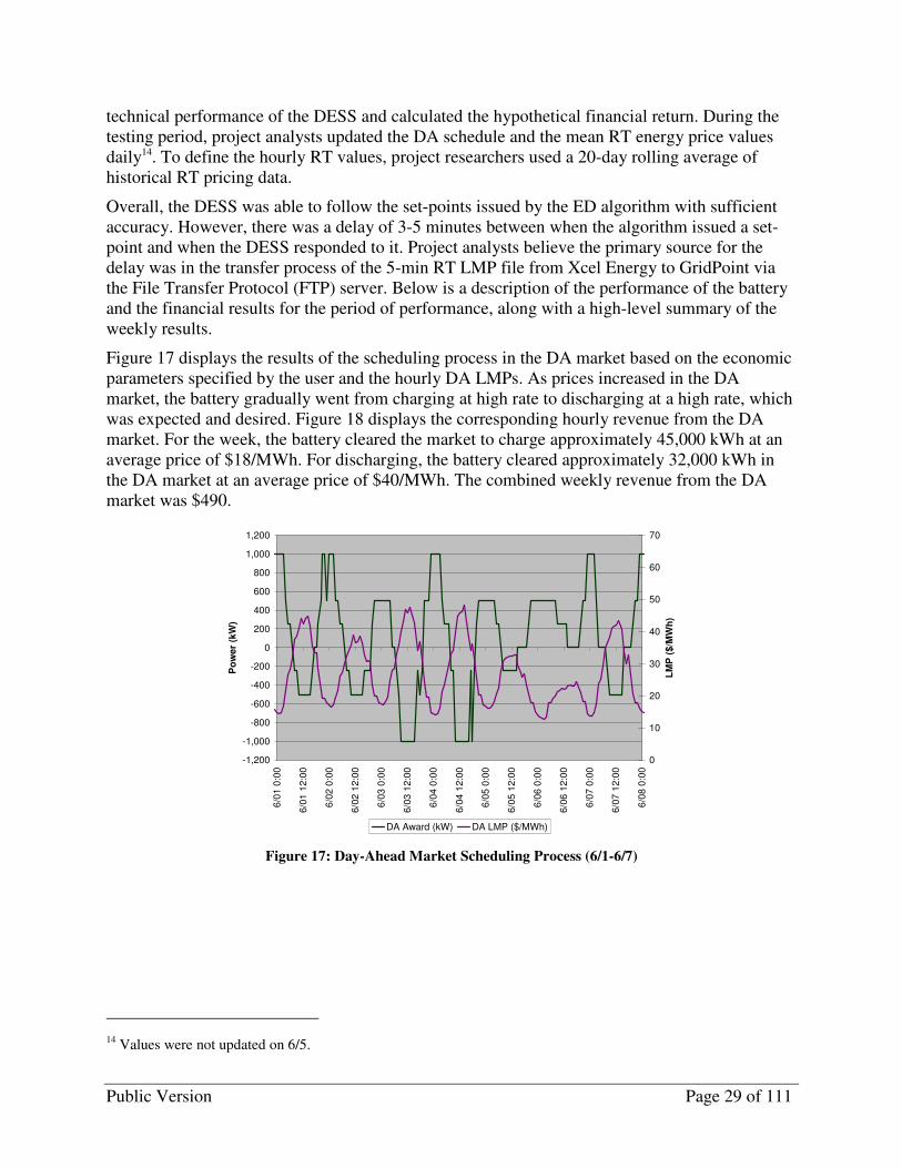
Figure 17 displays the results of the scheduling process in the DA market based on the economic parameters specified by the user and the hourly DA LMPs. As prices increased in the DA market, the battery gradually went from charging at high rate to discharging at a high rate, which was expected and desired. Figure 18 displays the corresponding hourly revenue from the DA market. For the week, the battery cleared the market to charge approximately 45,000 kWh at an average price of $18/MWh. For discharging, the battery cleared approximately 32,000 kWh in the DA market at an average price of $40/MWh. The combined weekly revenue from the DA market was $490.
-1,200
-1,000
-800
-600
-400
-200
0
200
400
600
800
1,000
1,200
6/0
1 0
:00
6/0
1 1
2:0
0
6/0
2 0
:00
6/0
2 1
2:0
0
6/0
3 0
:00
6/0
3 1
2:0
0
6/0
4 0
:00
6/0
4 1
2:0
0
6/0
5 0
:00
6/0
5 1
2:0
0
6/0
6 0
:00
6/0
6 1
2:0
0
6/0
7 0
:00
6/0
7 1
2:0
0
6/0
8 0
:00
Po
wer
(kW
)
0
10
20
30
40
50
60
70
LM
P (
$/M
Wh
)
DA Award (kW) DA LMP ($/MWh)
Figure 17: Day-Ahead Market Scheduling Process (6/1-6/7)
14 Values were not updated on 6/5.
Public Version Page 30 of 111
-$30
-$20
-$10
$0
$10
$20
$30
$40
$50
$60
$70
6/0
1 0
:00
6/0
1 1
2:0
0
6/0
2 0
:00
6/0
2 1
2:0
0
6/0
3 0
:00
6/0
3 1
2:0
0
6/0
4 0
:00
6/0
4 1
2:0
0
6/0
5 0
:00
6/0
5 1
2:0
0
6/0
6 0
:00
6/0
6 1
2:0
0
6/0
7 0
:00
6/0
7 1
2:0
0
6/0
8 0
:00
Figure 18: Day-Ahead Market Revenue (6/1-6/7)
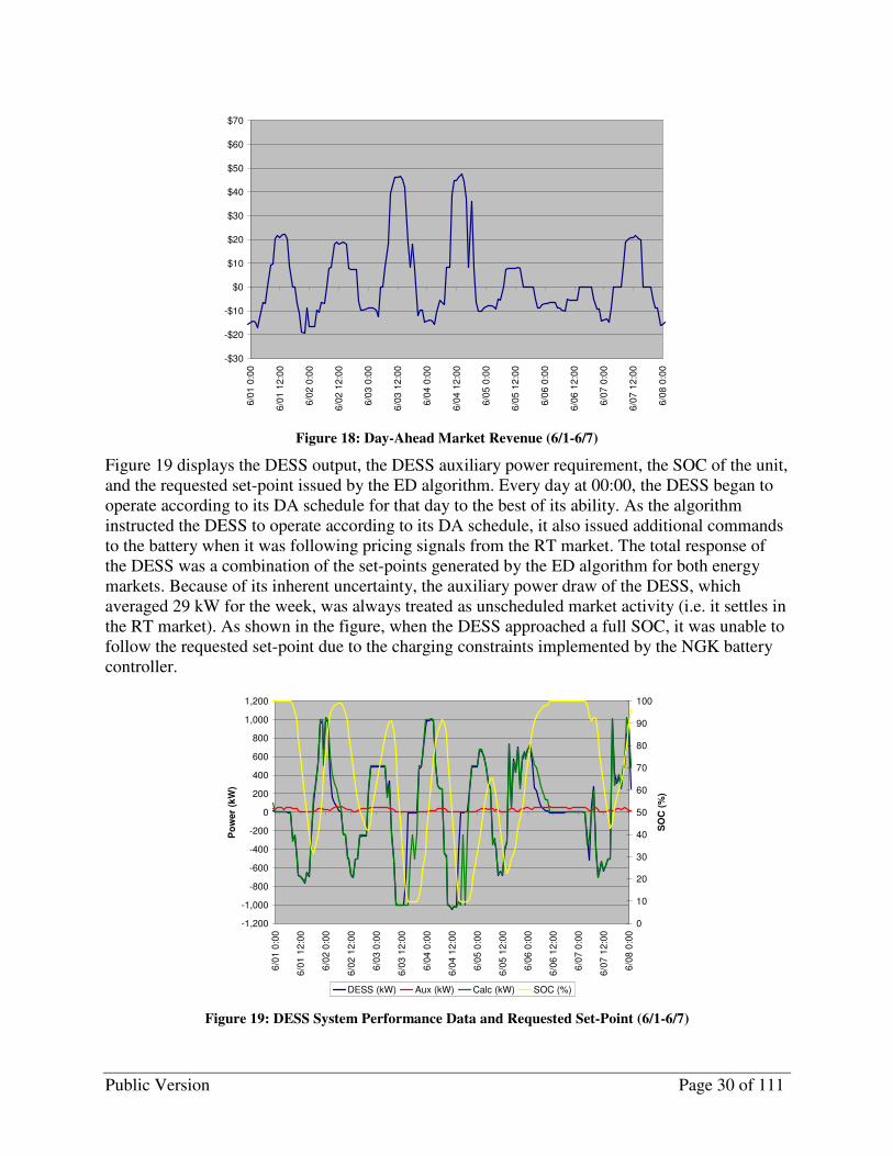
Figure 19 displays the DESS output, the DESS auxiliary power requirement, the SOC of the unit, and the requested set-point issued by the ED algorithm. Every day at 00:00, the DESS began to operate according to its DA schedule for that day to the best of its ability. As the algorithm instructed the DESS to operate according to its DA schedule, it also issued additional commands to the battery when it was following pricing signals from the RT market. The total response of the DESS was a combination of the set-points generated by the ED algorithm for both energy markets. Because of its inherent uncertainty, the auxiliary power draw of the DESS, which averaged 29 kW for the week, was always treated as unscheduled market activity (i.e. it settles in the RT market). As shown in the figure, when the DESS approached a full SOC, it was unable to follow the requested set-point due to the charging constraints implemented by the NGK battery controller.
-1,200
-1,000
-800
-600
-400
-200
0
200
400
600
800
1,000
1,200
6/0
1 0
:00
6/0
1 1
2:0
0
6/0
2 0
:00
6/0
2 1
2:0
0
6/0
3 0
:00
6/0
3 1
2:0
0
6/0
4 0
:00
6/0
4 1
2:0
0
6/0
5 0
:00
6/0
5 1
2:0
0
6/0
6 0
:00
6/0
6 1
2:0
0
6/0
7 0
:00
6/0
7 1
2:0
0
6/0
8 0
:00
Po
wer
(kW
)
0
10
20
30
40
50
60
70
80
90
100
SO
C (
%)
DESS (kW) Aux (kW) Calc (kW) SOC (%)
Figure 19: DESS System Performance Data and Requested Set-Point (6/1-6/7)
Public Version Page 31 of 111
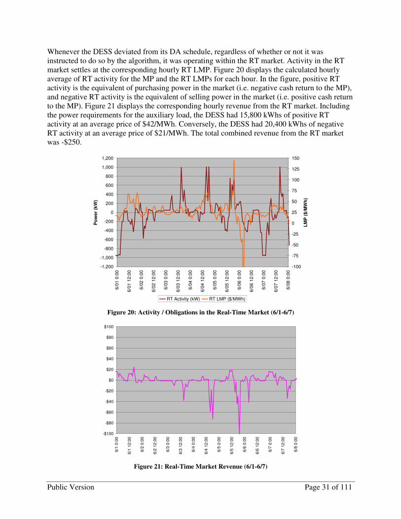
Whenever the DESS deviated from its DA schedule, regardless of whether or not it was instructed to do so by the algorithm, it was operating within the RT market. Activity in the RT market settles at the corresponding hourly RT LMP. Figure 20 displays the calculated hourly average of RT activity for the MP and the RT LMPs for each hour. In the figure, positive RT activity is the equivalent of purchasing power in the market (i.e. negative cash return to the MP), and negative RT activity is the equivalent of selling power in the market (i.e. positive cash return to the MP). Figure 21 displays the corresponding hourly revenue from the RT market. Including the power requirements for the auxiliary load, the DESS had 15,800 kWhs of positive RT activity at an average price of $42/MWh. Conversely, the DESS had 20,400 kWhs of negative RT activity at an average price of $21/MWh. The total combined revenue from the RT market was -$250.
-1,200
-1,000
-800
-600
-400
-200
0
200
400
600
800
1,000
1,200
6/0
1 0
:00
6/0
1 1
2:0
0
6/0
2 0
:00
6/0
2 1
2:0
0
6/0
3 0
:00
6/0
3 1
2:0
0
6/0
4 0
:00
6/0
4 1
2:0
0
6/0
5 0
:00
6/0
5 1
2:0
0
6/0
6 0
:00
6/0
6 1
2:0
0
6/0
7 0
:00
6/0
7 1
2:0
0
6/0
8 0
:00
Po
we
r (k
W)
-100
-75
-50
-25
0
25
50
75
100
125
150
LM
P (
$/M
Wh
)
RT Activity (kW) RT LMP ($/MWh)
Figure 20: Activity / Obligations in the Real-Time Market (6/1-6/7)
-$100
-$80
-$60
-$40
-$20
$0
$20
$40
$60
$80
$100
6/1
0:0
0
6/1
12
:00
6/2
0:0
0
6/2
12
:00
6/3
0:0
0
6/3
12
:00
6/4
0:0
0
6/4
12
:00
6/5
0:0
0
6/5
12
:00
6/6
0:0
0
6/6
12
:00
6/7
0:0
0
6/7
12
:00
6/8
0:0
0
Figure 21: Real-Time Market Revenue (6/1-6/7)
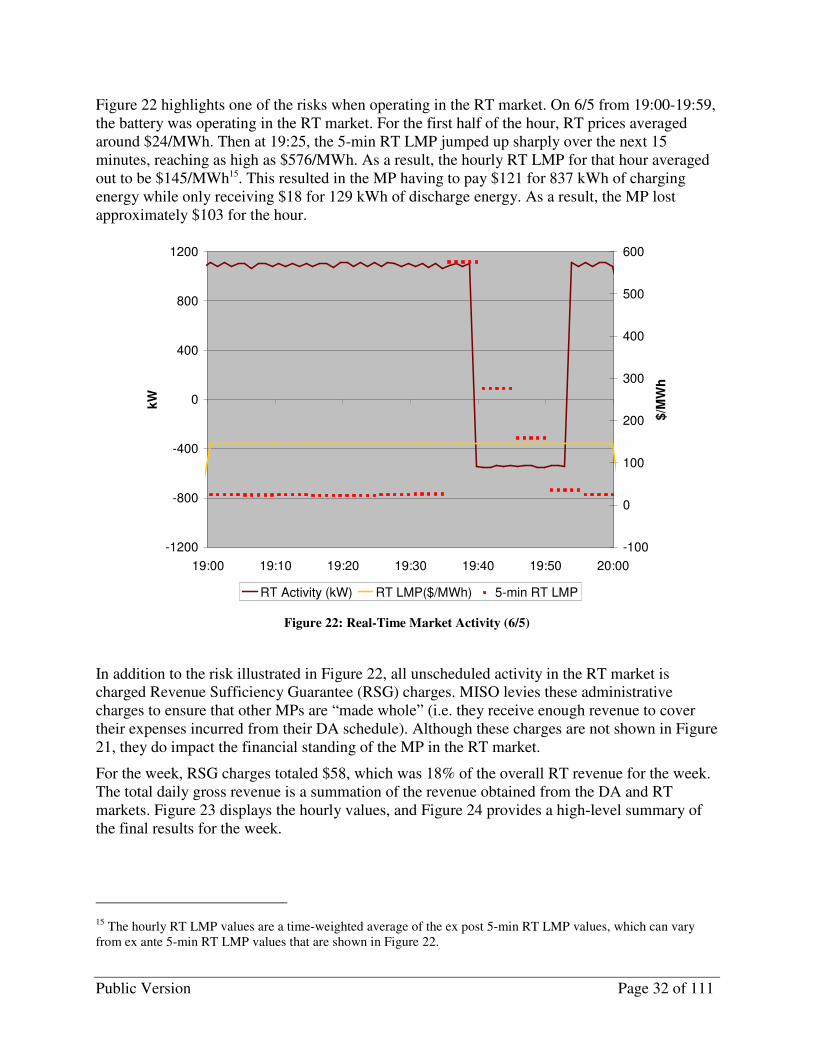
Public Version Page 32 of 111
Figure 22 highlights one of the risks when operating in the RT market. On 6/5 from 19:00-19:59, the battery was operating in the RT market. For the first half of the hour, RT prices averaged around $24/MWh. Then at 19:25, the 5-min RT LMP jumped up sharply over the next 15 minutes, reaching as high as $576/MWh. As a result, the hourly RT LMP for that hour averaged out to be $145/MWh15. This resulted in the MP having to pay $121 for 837 kWh of charging energy while only receiving $18 for 129 kWh of discharge energy. As a result, the MP lost approximately $103 for the hour.
-1200
-800
-400
0
400
800
1200
19:00 19:10 19:20 19:30 19:40 19:50 20:00
kW
-100
0
100
200
300
400
500
600
$/M
Wh
RT Activity (kW) RT LMP($/MWh) 5-min RT LMP
Figure 22: Real-Time Market Activity (6/5)
In addition to the risk illustrated in Figure 22, all unscheduled activity in the RT market is charged Revenue Sufficiency Guarantee (RSG) charges. MISO levies these administrative charges to ensure that other MPs are “made whole” (i.e. they receive enough revenue to cover their expenses incurred from their DA schedule). Although these charges are not shown in Figure 21, they do impact the financial standing of the MP in the RT market.
For the week, RSG charges totaled $58, which was 18% of the overall RT revenue for the week. The total daily gross revenue is a summation of the revenue obtained from the DA and RT markets. Figure 23 displays the hourly values, and Figure 24 provides a high-level summary of the final results for the week.
15 The hourly RT LMP values are a time-weighted average of the ex post 5-min RT LMP values, which can vary from ex ante 5-min RT LMP values that are shown in Figure 22.
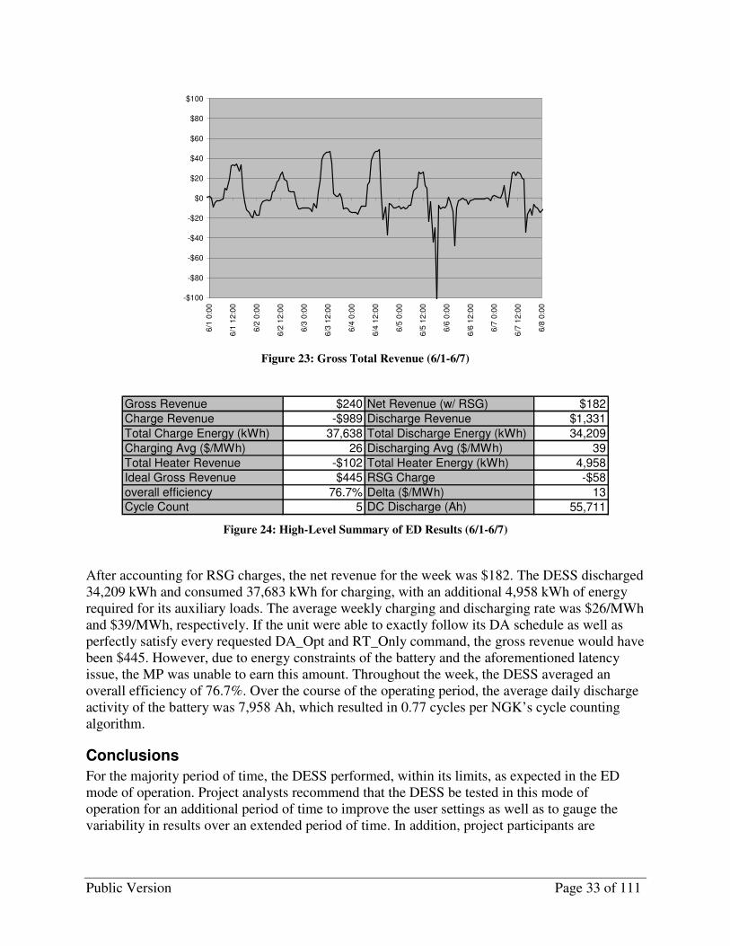
Public Version Page 33 of 111
-$100
-$80
-$60
-$40
-$20
$0
$20
$40
$60
$80
$100
6/1
0:0
0
6/1
12:0
0
6/2
0:0
0
6/2
12:0
0
6/3
0:0
0
6/3
12:0
0
6/4
0:0
0
6/4
12:0
0
6/5
0:0
0
6/5
12:0
0
6/6
0:0
0
6/6
12:0
0
6/7
0:0
0
6/7
12:0
0
6/8
0:0
0
Figure 23: Gross Total Revenue (6/1-6/7)
Gross Revenue $240 Net Revenue (w/ RSG) $182
Charge Revenue -$989 Discharge Revenue $1,331
Total Charge Energy (kWh) 37,638 Total Discharge Energy (kWh) 34,209
Charging Avg ($/MWh) 26 Discharging Avg ($/MWh) 39
Total Heater Revenue -$102 Total Heater Energy (kWh) 4,958Ideal Gross Revenue $445 RSG Charge -$58
overall efficiency 76.7% Delta ($/MWh) 13Cycle Count 5 DC Discharge (Ah) 55,711
Figure 24: High-Level Summary of ED Results (6/1-6/7)
After accounting for RSG charges, the net revenue for the week was $182. The DESS discharged 34,209 kWh and consumed 37,683 kWh for charging, with an additional 4,958 kWh of energy required for its auxiliary loads. The average weekly charging and discharging rate was $26/MWh and $39/MWh, respectively. If the unit were able to exactly follow its DA schedule as well as perfectly satisfy every requested DA_Opt and RT_Only command, the gross revenue would have been $445. However, due to energy constraints of the battery and the aforementioned latency issue, the MP was unable to earn this amount. Throughout the week, the DESS averaged an overall efficiency of 76.7%. Over the course of the operating period, the average daily discharge activity of the battery was 7,958 Ah, which resulted in 0.77 cycles per NGK’s cycle counting algorithm.
Conclusions
For the majority period of time, the DESS performed, within its limits, as expected in the ED mode of operation. Project analysts recommend that the DESS be tested in this mode of operation for an additional period of time to improve the user settings as well as to gauge the variability in results over an extended period of time. In addition, project participants are

Public Version Page 34 of 111
interested in controlling the battery strictly off set-points derived from the RT market to determine the corresponding value achieved by the DESS.
Currently, the potential for arbitrage in the MISO market at the selected CPNode is limited as shown by the small spread in the average charge and discharge rates. However, project analysts may obtain improved results by optimizing the ED algorithm user settings and defining the expected DA and RT energy prices with less error. Notwithstanding any improvements obtained by optimizing the ED algorithm settings, it is difficult for a MP to optimize the operation of a bulk storage device in the MISO market because of its inherent energy constraints and the potential to be exposed to market risk in a variety of manners. Project analysts should work closely with MISO to discuss how a market resource such as the DESS would be best utilized in the energy market.
Table 11 lists the system performance data of interest for the one week testing period of the Economic Dispatch mode of operation. During this testing period, the average mileage of the DESS was 25,508 kW/day. Again, the battery never exceeded more than one discharge cycle in any given day, averaging 0.77 cycles over the week. The average daily auxiliary energy requirement was 709 kWh/day. The overall efficiency of the DESS with and without the auxiliary energy requirements averaged 78.1% and 87.3%, respectively.
Table 11: Economic Dispatch System Performance Data Statistics Summary
Mode
Mileage
(kW/day)
Daily
Discharge
Cycle
Usage
Aux Energy
Requirement
(kWh/day) η1 η2
Economic Dispatch 25,508 0.77 709 78.1% 87.3%

Public Version Page 35 of 111
Supplemental Information for ED Mode
Figure 25 provides a detailed breakdown of the system performance data for the ED mode of operation, with a description of the categories located below.
% DA_Only Operation Mode 81% % DA_Opt Operation Mode 11%
% Rogue Operation Mode 5% % RT_Only Operation Mode 9%
% Requested Idle 6% % Actual Idle 24%
% DA_Only Charge Energy 77.1% % DA_Only Discharge Energy 78.7%
% DA_Opt Charge Energy 3.1% % DA_Opt Discharge Energy 12.1%
% RT_Only Charge Energy 18.9% % RT_Only Discharge Energy 6.8%
% Rogue Charge Energy 0.8% % Rogue Discharge Energy 2.3%% True Up Charge Energy
(over) 1.8%
% True Up Discharge Energy
(over) 2.4%% True Up Charge Energy
(under) 44.4%
% True Up Discharge Energy
(under) 17.7%
DA_Only Charge Rev -$791 DA_Only Discharge Revenue $1,281
DA_Opt Charge Revenue -$1 DA_Opt Discharge Revenue $187
RT_Only Charge Revenue -$380 RT_Only Discharge Revenue $106
Rogue Charge Revenue -$9 Rogue Discharge Revenue $20True Up Charge Revenue
(over) -$14
True Up Discharge Revenue
(over) $34True Up Charge Revenue
(under) $206
True Up Discharge Revenue
(under) -$298DA_Only Charge Avg Price
($/MWh) 28
DA_Only Discharge Avg Price
($/MWh) 46DA_Opt Avg Charge Price
($/MWh) 16
DA_Opt Avg Discharge Price
($/MWh) 36RT_Only Charge Avg Price
($/MWh) 33
RT_Only Discharge Avg Price
($/MWh) 24Rogue Charge Avg Price
($/MWh) 17
Rogue Discharge Avg Price
($/MWh) 19True Up Charge Avg Price
($/MWh) (over) 21
True Up Discharge Avg Price
($/MWh) (over) 38True Up Charge Avg Price
($/MWh) (under) 19
True Up Discharge Avg Price
($/MWh) (under) 40DA Charge Award (kWh) 45000 DA Discharge Award (kWh) -32000DA Charge Award Avg Rate
($/kWh) 18
DA Discharge Award Avg Rate
($/kWh) 40
DA Charge Penalty $83 DA Discharge Penalty $66
Figure 25: High-Level Summary of Weekly ED Results (6/1-6/7)
The “% ‘mode’ Operation Mode” categories (e.g. ‘DA_Only’ Operation mode) provide the amount of time the battery was in each particular mode of operation. The DA_Only operation mode is active whenever the battery is operating as a result of it trying to meet its DA obligation16. Conversely, the DA_Opt operation mode is active when the battery has a DA obligation for that hour and is operating in the RT market. Finally, the RT_Only operation mode is active when there is no DA obligation for that hour but the battery is operating in the RT
16 If the battery has a DA obligation but is not operating, it is not considered to be in the DA_Only mode.

Public Version Page 36 of 111
market. The Rogue operation mode is a catch-all that accounts for all the unexpected and delayed activity of the DESS.
The “% Requested Idle” category tracks the amount of time that the ED algorithm instructed the battery to be idle (i.e. to not produce or consume any power). Conversely, the “% Actual Idle” category trends the actual amount of time the DESS was idle, either due to energy constraints of the battery, system alarms, or other factors affecting performance. Note that the modes do not add up to 100% because there are some overlaps between the modes. First, whenever the battery is in the DA_Opt mode, it is also in the DA_Only mode. Second, delayed operation of the DESS may be accounted for by both the “% Requested Idle” and “% Rogue Operation Mode” categories.
The “% ‘mode’ Charge / Discharge Energy” categories trend the respective amount of charge/discharge energy that occurred while in that mode relative to the total amount of charge/discharge energy over the entire period of performance17. For example, the “% RT_Only Charge Energy” category shows a value of 18.92%; therefore, approximately 7,100 kWh of charge energy was acquired while the battery was in the RT_Only mode. The “% True Up Charge / Discharge Energy (over)” categories track the amount of energy that the MP either bought in the RT market when it charged at a rate greater than expected or sold in the RT market when it discharged at a rate greater than expected. The “% True Up Charge / Discharge Energy (under)” categories track the amount of energy that the MP either sold in the RT market when it charged at a rate less than expected or bought in the RT market when it discharged at a rate less than expected. For example, the “% True Up Charge Energy (over)” value was 1.8%, which means that the DESS exceeded its DA schedule for charging by approximately 677 kWh for the week. The “% True Up Discharge Energy (under)” value was 17.7%, which means that the DESS was short on its obligation to serve as a generator for a total of approximately 6,050 kWh.
The “‘mode’ Charge / Discharge Revenue” categories calculate the respective amount of charge or discharge revenue that occurred while in that mode. For example, the DESS earned $1,281 by discharging in the DA_Only mode but had to pay $298 to fulfill its DA obligation as a generator. The “‘mode’ Charge/Discharge Avg Price ($/MWh)” categories give the average rate that the DESS paid or earned while in that mode. It is simply the absolute value of the respective revenue divided by the respective amount of energy.
The “DA Charge/Discharge Penalty” categories calculate the penalty a MP incurs by having to true up the MP’s DA position in the RT market. Because this is a penalty, a positive value equates to the MP having to either pay more or earn less in the RT market than the MP would have in the DA market. For example, if the unit is scheduled in the DA market to charge at 500 kW but is actually charging at 800 kW and the RT price is less than the DA LMP, the penalty is negative because this is a benefit to the MP. Conversely, if the unit is scheduled in the DA market to discharge at 500 kW but is only discharging at 250 kW and the RT price is more than the DA LMP, then the penalty is positive. The DA Charge Penalty and Discharge Penalty for the week of 6/1-6/7 were $83 and $66, respectively.
17 Respective energy amounts for each mode of operation were estimated based on instantaneous energy values.

Public Version Page 37 of 111
Frequency Regulation
Introduction
One value proposition in the W2B Test Plan is to evaluate the ability of large-scale battery storage technology to provide the market service of frequency regulation both as a load and a generator. Under this mode, the DESS follows a frequency regulation signal derived from changes in the Area Control Error (ACE) for the MISO market.
Theory
Ancillary services are required services that support generation and transmission functions for the bulk electric power grid. One type of ancillary service, frequency regulation, is primarily intended to assist a balancing authority in maintaining its ACE to within the limits prescribed by the North American Electric Reliability Corporation (NERC) control performance standards.
Positive ACE represents an over-generation situation, where larger ACE values mean greater amounts of over-generation. Conversely, negative ACE represents an under-generation situation, where larger negative ACE values mean greater amounts of under-generation. A regulating resource is defined as an online resource (e.g., generation, storage, or responsive load) connected to an Automatic Generation Control (AGC) system with the intent to balance the random and rapid fluctuations in generation and/or load on an intra-minute basis [Kirby].
Because regulation set-points are typically updated every 2-6 seconds, units providing regulation typically have good ramping capability. Regulating units that can respond to control signals in a timely and accurate manner enable a balancing authority to reduce the overall amount of regulating reserves it must procure, thereby increasing system efficiency [Makarov]. Indeed, some storage advocates argue that faster responding resources should be compensated more than traditional generation-based ancillary service resources.
Below is a description of the logic used by the NSP Energy Management System (EMS) to generate the frequency regulation signal for the battery. The code calls for the battery to charge whenever the ACE is greater than the maximum allowed value, discharge whenever the ACE is less than the minimum allowed value, and be idle whenever the ACE is within the allowed dead-band range. NSP EMS updates the control set-point every 4 seconds. The PCS still honors all charging and discharge constraints for the storage device while in this mode. Please refer to the architecture discussion on page 98 for an overview of the data flows and a description of the variables listed below.
Positive MISO ACE (i.e., over generation):
If MISO_ACE > AceDb_BatU, calculated regulation signal will be
Calculated Setpointi = Scaling_factor * (MISO_ACE – AceDB_BatU).
The charge command sent to the battery will be
Target Poweri = Target Poweri-1 + min (Calculated Setpointi, positive ramp rate / 60 * AGC cycle time)
If the charge command to be sent to the battery is greater than the maximum allowed limit, then the battery will be commanded to charge at its maximum allowed rate.
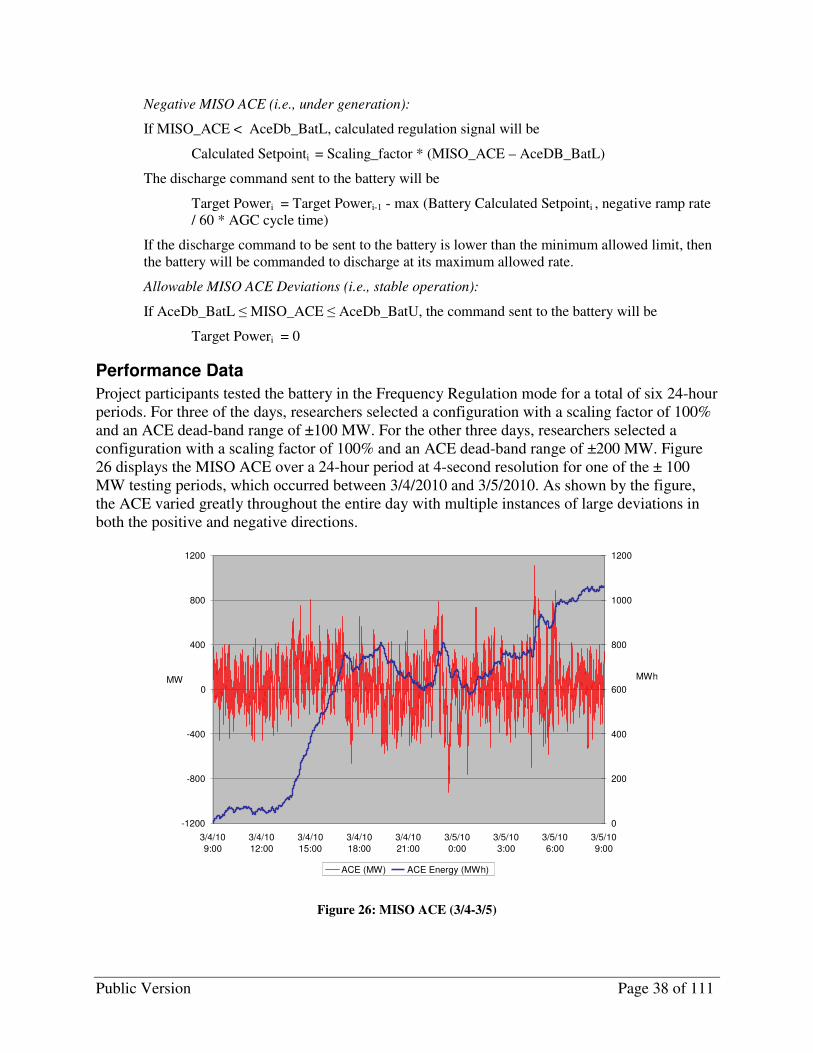
Public Version Page 38 of 111
Negative MISO ACE (i.e., under generation):
If MISO_ACE < AceDb_BatL, calculated regulation signal will be
Calculated Setpointi = Scaling_factor * (MISO_ACE – AceDB_BatL)
The discharge command sent to the battery will be
Target Poweri = Target Poweri-1 - max (Battery Calculated Setpointi , negative ramp rate / 60 * AGC cycle time)
If the discharge command to be sent to the battery is lower than the minimum allowed limit, then the battery will be commanded to discharge at its maximum allowed rate.
Allowable MISO ACE Deviations (i.e., stable operation):
If AceDb_BatL ≤ MISO_ACE ≤ AceDb_BatU, the command sent to the battery will be
Target Poweri = 0
Performance Data
Project participants tested the battery in the Frequency Regulation mode for a total of six 24-hour periods. For three of the days, researchers selected a configuration with a scaling factor of 100% and an ACE dead-band range of ±100 MW. For the other three days, researchers selected a configuration with a scaling factor of 100% and an ACE dead-band range of ±200 MW. Figure 26 displays the MISO ACE over a 24-hour period at 4-second resolution for one of the ± 100 MW testing periods, which occurred between 3/4/2010 and 3/5/2010. As shown by the figure, the ACE varied greatly throughout the entire day with multiple instances of large deviations in both the positive and negative directions.
Figure 26: MISO ACE (3/4-3/5)
-1200
-800
-400
0
400
800
1200
3/4/10 9:00
3/4/10 12:00
3/4/10 15:00
3/4/10 18:00
3/4/10 21:00
3/5/10 0:00
3/5/10 3:00
3/5/10 6:00
3/5/10 9:00
MW
0
200
400
600
800
1000
1200
MWh
ACE (MW) ACE Energy (MWh)
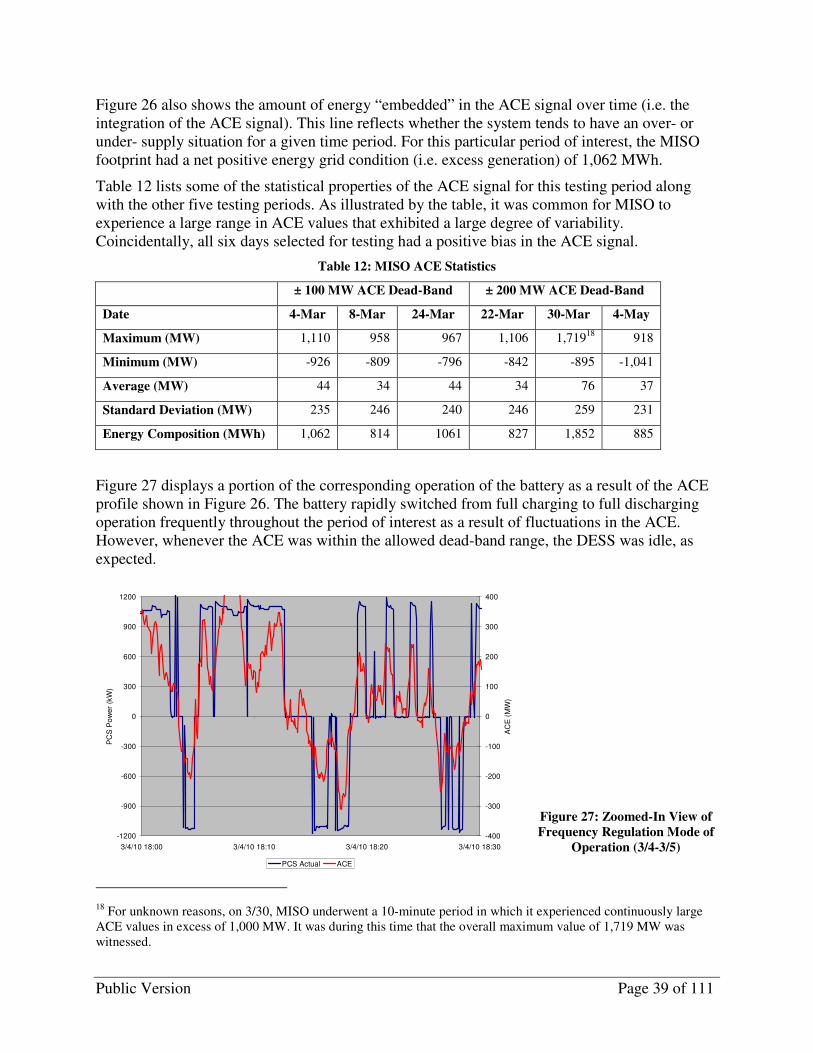
Public Version Page 39 of 111
Figure 26 also shows the amount of energy “embedded” in the ACE signal over time (i.e. the integration of the ACE signal). This line reflects whether the system tends to have an over- or under- supply situation for a given time period. For this particular period of interest, the MISO footprint had a net positive energy grid condition (i.e. excess generation) of 1,062 MWh.
Table 12 lists some of the statistical properties of the ACE signal for this testing period along with the other five testing periods. As illustrated by the table, it was common for MISO to experience a large range in ACE values that exhibited a large degree of variability. Coincidentally, all six days selected for testing had a positive bias in the ACE signal.
Table 12: MISO ACE Statistics
± 100 MW ACE Dead-Band ± 200 MW ACE Dead-Band
Date 4-Mar 8-Mar 24-Mar 22-Mar 30-Mar 4-May
Maximum (MW) 1,110 958 967 1,106 1,71918 918
Minimum (MW) -926 -809 -796 -842 -895 -1,041
Average (MW) 44 34 44 34 76 37
Standard Deviation (MW) 235 246 240 246 259 231
Energy Composition (MWh) 1,062 814 1061 827 1,852 885
Figure 27 displays a portion of the corresponding operation of the battery as a result of the ACE profile shown in Figure 26. The battery rapidly switched from full charging to full discharging operation frequently throughout the period of interest as a result of fluctuations in the ACE. However, whenever the ACE was within the allowed dead-band range, the DESS was idle, as expected.
Figure 27: Zoomed-In View of
Frequency Regulation Mode of
Operation (3/4-3/5)
18 For unknown reasons, on 3/30, MISO underwent a 10-minute period in which it experienced continuously large ACE values in excess of 1,000 MW. It was during this time that the overall maximum value of 1,719 MW was witnessed.
-1200
-900
-600
-300
0
300
600
900
1200
3/4/10 18:00 3/4/10 18:10 3/4/10 18:20 3/4/10 18:30
PC
S P
ow
er
(kW
)
-400
-300
-200
-100
0
100
200
300
400
AC
E (
MW
)
PCS Actual ACE

Public Version Page 40 of 111
Overall, the PCS generally behaved as expected based on the logic specified by the NSP EMS regulation code for all six operating periods. However, while in this mode, the PCS frequently and randomly issued temporary Inhibit Alarms (approximately 50 to 80 alarms) lasting between 4-8 seconds19. The dead-band setting did not appear to be a factor in the number of alarms issued. According to S&C, the Inhibit Alarms were the result of DC Over-Voltages that occurred when the DESS rapidly changed from charge or discharge to zero. S&C states the newest version of the PCS software will account for this condition and will not issue an alarm as a result.
Table 13 lists the primary DESS performance statistics for the Frequency Regulation mode of operation for the profile shown in Figure 26 along with the other testing periods. As expected, for a larger ACE dead-band window the DESS was less active. In the ±100 MW scenarios, the average mileage20 was 2,012,252 kW/day and the DESS was idle for approximately 7.5 hours on average. In addition, the maximum idle duration period varied between 205-272 seconds. In the ±200 MW scenarios, the average mileage was 1,543,603 kW/day, and the DESS was idle for approximately 14.2 hours on average. Furthermore, the maximum idle duration period varied between 641-673 seconds. Maximum ramp-up and ramp-down rates experienced by the DESS were similar for both testing configurations. Moreover, the maximum amount of required charge and discharge energy along with the cumulative amount of energy absorbed or provided by the DESS appeared to be more dependent on the ACE signal and less on the dead-band setting.
Table 13: DESS Frequency Regulation Performance Statistics (3/4-3/5)
± 100 MW ACE Dead-Band ± 200 MW ACE Dead-Band
Starting Date 4-Mar 8-Mar 24-Mar 22-Mar 30-Mar 4-May
Mileage (kW/day) 2,102,876 1,873,935 2,059,944 1,597,289 1,556,917 1,476,602
Max Ramp Rate Up
(kW/min) 24 19 18 19 19 18
Max Ramp Rate Down
(kW/min) -23 -18 -26 -19 -24 -19
% Time Spent Idle 33.1% 30.1% 31.3% 56.5% 58.8% 61.9%
Maximum Idle Duration
Period (sec) 226 205 272 641 648 673
Maximum Required
Charge Energy - 60 min
(kWh) 748 680 735 545 494 515
Maximum Required
Discharge Energy - 60 min
(kWh) 439 505 507 357 135 342
Maximum Required
Charge Energy - 30 min
(kWh) 465 395 456 388 423 437
19 For an Inhibit or Trip Alarm, PCS reports the SOC and the maximum discharge capacity as 0.
20 Mileage is the metric used to gauge the “stress” of the duty profile imposed on the battery. It is the cumulative sum of the absolute value of the change in PCS power settings from one time step to the next. As a reference, a repeating 24-hr duty profile consisting of 5 minutes at 1,000 kW, 5 minutes at 0 kW, 5 minutes at -1,000 kW, and 5 minutes at 0 kW has a mileage of 288,000 kW/day.

Public Version Page 41 of 111
± 100 MW ACE Dead-Band ± 200 MW ACE Dead-Band
Starting Date 4-Mar 8-Mar 24-Mar 22-Mar 30-Mar 4-May
Maximum Required
Discharge Energy - 30 min
(kWh) 447 338 323 206 167 340
Maximum Required
Charge Energy - 15 min
(kWh) 252 250 249 251 251 244
Maximum Required
Discharge Energy - 15 min
(kWh) 258 223 229 233 146 256
24-Hr Cumulative Energy
Usage (kWh) 3,466 1,514 2,991 2,241 3,947 2,205
Total Battery Ampere-
Hour Discharge (DC Ah) 10,912 13,190 11,360 6,287 4,635 5,875
Figure 28 displays the energy requirements of the DESS and its corresponding change in state of charge for the 3/4-3/5 testing period. As shown in the figure, over the 24-hour period the DESS received a net charge of approximately 3,500 kWh. However, the DESS was never unable to provide either regulation-up or regulation-down capability at its nominal capacity due to energy limitations.
0
500
1000
1500
2000
2500
3000
3500
4000
3/4/109:00
3/4/1012:00
3/4/1015:00
3/4/1018:00
3/4/1021:00
3/5/100:00
3/5/103:00
3/5/106:00
3/5/109:00
En
erg
y R
eq
uir
em
en
ts (
kW
h)
0%
20%
40%
60%
80%
100%
Sta
te o
f C
harg
e
Energy SOC
Figure 28: Frequency Regulation Energy Requirements and DESS SOC (3/4-3/5)
However, this was not the case for all the testing periods. Figure 29 displays the energy requirements of the DESS and its corresponding change in state of charge for the 3/24-3/25 testing period. From 6:39-8:34, the DESS was unable to provide full regulation-down capability due to the charging restraints employed by the NGK battery controller whenever the battery approaches a full state of charge. At 6:39 with a SOC of 96.4%, the maximum charge capacity of the DESS reduced to 962 kW. At 6:51 with a SOC of 97.2%, it dropped to 825 kW. Fortunately, the regulation set-points started to instruct the DESS to discharge, which alleviated the energy
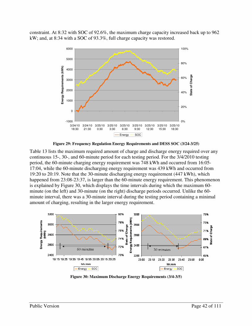
Public Version Page 42 of 111
constraint. At 8:32 with SOC of 92.6%, the maximum charge capacity increased back up to 962 kW; and, at 8:34 with a SOC of 93.3%, full charge capacity was restored.
-1000
0
1000
2000
3000
4000
5000
6000
3/24/1018:30
3/24/1021:30
3/25/100:30
3/25/103:30
3/25/106:30
3/25/109:30
3/25/1012:30
3/25/1015:30
3/25/1018:30
En
erg
y R
eq
uir
em
en
ts (
kW
h)
0%
20%
40%
60%
80%
100%
Sta
te o
f C
harg
e
Energy SOC
Figure 29: Frequency Regulation Energy Requirements and DESS SOC (3/24-3/25)
Table 13 lists the maximum required amount of charge and discharge energy required over any continuous 15-, 30-, and 60-minute period for each testing period. For the 3/4/2010 testing period, the 60-minute charging energy requirement was 748 kWh and occurred from 16:05-17:04, while the 60-minute discharging energy requirement was 439 kWh and occurred from 19:20 to 20:19. Note that the 30-minute discharging energy requirement (447 kWh), which happened from 23:08-23:37, is larger than the 60-minute energy requirement. This phenomenon is explained by Figure 30, which displays the time intervals during which the maximum 60-minute (on the left) and 30-minute (on the right) discharge periods occurred. Unlike the 60-minute interval, there was a 30-minute interval during the testing period containing a minimal amount of charging, resulting in the larger energy requirement.
Figure 30: Maximum Discharge Energy Requirements (3/4-3/5)
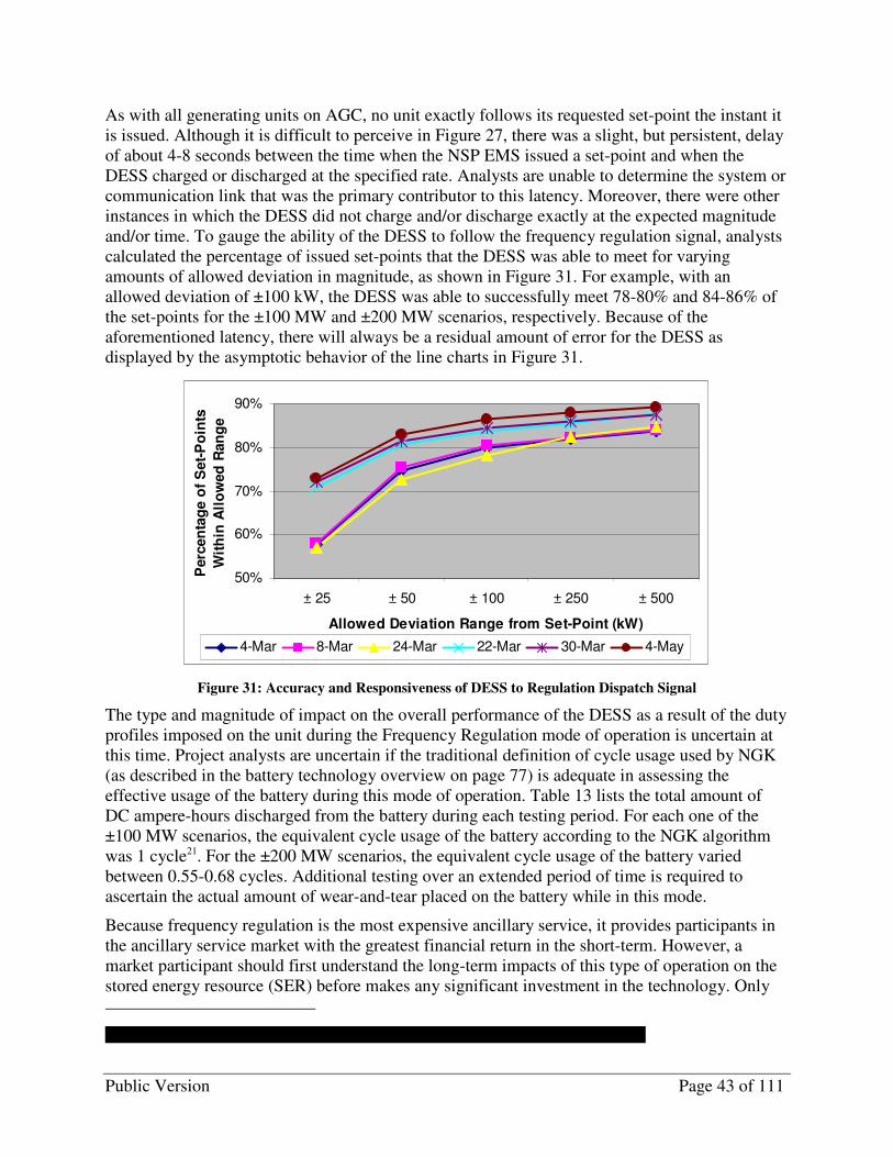
Public Version Page 43 of 111
As with all generating units on AGC, no unit exactly follows its requested set-point the instant it is issued. Although it is difficult to perceive in Figure 27, there was a slight, but persistent, delay of about 4-8 seconds between the time when the NSP EMS issued a set-point and when the DESS charged or discharged at the specified rate. Analysts are unable to determine the system or communication link that was the primary contributor to this latency. Moreover, there were other instances in which the DESS did not charge and/or discharge exactly at the expected magnitude and/or time. To gauge the ability of the DESS to follow the frequency regulation signal, analysts calculated the percentage of issued set-points that the DESS was able to meet for varying amounts of allowed deviation in magnitude, as shown in Figure 31. For example, with an allowed deviation of ±100 kW, the DESS was able to successfully meet 78-80% and 84-86% of the set-points for the ±100 MW and ±200 MW scenarios, respectively. Because of the aforementioned latency, there will always be a residual amount of error for the DESS as displayed by the asymptotic behavior of the line charts in Figure 31.
50%
60%
70%
80%
90%
± 25 ± 50 ± 100 ± 250 ± 500
Allowed Deviation Range from Set-Point (kW)
Perc
en
tag
e o
f S
et-
Po
ints
Wit
hin
All
ow
ed
Ran
ge
4-Mar 8-Mar 24-Mar 22-Mar 30-Mar 4-May
Figure 31: Accuracy and Responsiveness of DESS to Regulation Dispatch Signal
The type and magnitude of impact on the overall performance of the DESS as a result of the duty profiles imposed on the unit during the Frequency Regulation mode of operation is uncertain at this time. Project analysts are uncertain if the traditional definition of cycle usage used by NGK (as described in the battery technology overview on page 77) is adequate in assessing the effective usage of the battery during this mode of operation. Table 13 lists the total amount of DC ampere-hours discharged from the battery during each testing period. For each one of the ±100 MW scenarios, the equivalent cycle usage of the battery according to the NGK algorithm was 1 cycle21. For the ±200 MW scenarios, the equivalent cycle usage of the battery varied between 0.55-0.68 cycles. Additional testing over an extended period of time is required to ascertain the actual amount of wear-and-tear placed on the battery while in this mode.
Because frequency regulation is the most expensive ancillary service, it provides participants in the ancillary service market with the greatest financial return in the short-term. However, a market participant should first understand the long-term impacts of this type of operation on the stored energy resource (SER) before makes any significant investment in the technology. Only
21According to NGK, the nominal discharge capacity of the 1 MW NaS battery is 13,200 Ah

Public Version Page 44 of 111
after this information is ascertained will the asset owner be able to determine if this operational mode is still cost-effective overall in the long run. The University of Minnesota will perform a preliminary investigation on this topic and report on its findings in their report to Xcel Energy, which is scheduled to be delivered June 2011.
Conclusions
The DESS performed well in the Frequency Regulation mode of operation. Despite a delay of 4-8 seconds in the routing of the signal, the storage device responded promptly and accurately once it did receive the control set-point. When providing regulation, the DESS displayed excellent ramping capabilities on a continuous basis by being able to effectively follow the rapidly changing set-points that NSP EMS issued. Additional testing and close collaboration with NGK is required to assess the impact this mode has on the long-term performance and lifespan of the unit. Once greater clarity around this issue is obtained, a market participant can weigh the risk of degradation in future system performance and/or expected life with the value obtained by offering the unit to provide regulating reserves in MISO’s Ancillary Service Market (ASM). Xcel Energy has plans to officially submit the DESS into the MISO ASM in the summer of 2010 and will report on the results.
Table 14 lists the system performance data of interest for the Frequency Regulation testing period. The average mileage of the DESS was 1,777,928 kW/day. The battery never exceeded more than one discharge cycle in any given day, averaging 0.81 cycles over the two testing variations. The average daily auxiliary energy requirement was 500 kWh/day. The overall efficiency of the DESS with and without the auxiliary energy requirements averaged 78.9% and 86.8%, respectively.
Table 14: Frequency Regulation System Performance Data Statistics Summary
Mode
ACE
Dead-
band
Mileage
(kW/day)
Daily
Discharge
Cycle
Usage
Aux Energy
Requirement
(kWh/day) η1 η2
Frequency Regulation 100 2,012,252 1.00 309 83.2% 86.1%
Frequency Regulation 200 1,543,603 0.63 690 74.6% 87.4%
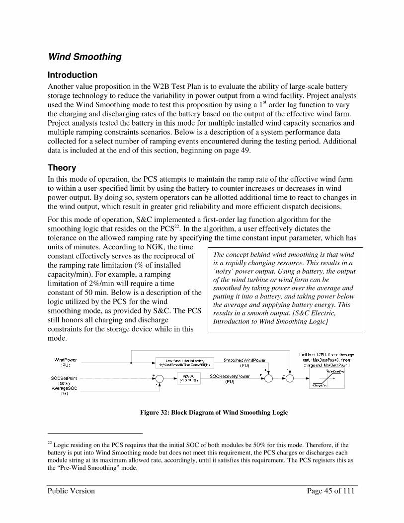
Public Version Page 45 of 111
Wind Smoothing
Introduction
Another value proposition in the W2B Test Plan is to evaluate the ability of large-scale battery storage technology to reduce the variability in power output from a wind facility. Project analysts used the Wind Smoothing mode to test this proposition by using a 1st order lag function to vary the charging and discharging rates of the battery based on the output of the effective wind farm. Project analysts tested the battery in this mode for multiple installed wind capacity scenarios and multiple ramping constraints scenarios. Below is a description of a system performance data collected for a select number of ramping events encountered during the testing period. Additional data is included at the end of this section, beginning on page 49.
Theory
In this mode of operation, the PCS attempts to maintain the ramp rate of the effective wind farm to within a user-specified limit by using the battery to counter increases or decreases in wind power output. By doing so, system operators can be allotted additional time to react to changes in the wind output, which result in greater grid reliability and more efficient dispatch decisions.
For this mode of operation, S&C implemented a first-order lag function algorithm for the smoothing logic that resides on the PCS22. In the algorithm, a user effectively dictates the tolerance on the allowed ramping rate by specifying the time constant input parameter, which has units of minutes. According to NGK, the time constant effectively serves as the reciprocal of the ramping rate limitation (% of installed capacity/min). For example, a ramping limitation of 2%/min will require a time constant of 50 min. Below is a description of the logic utilized by the PCS for the wind smoothing mode, as provided by S&C. The PCS still honors all charging and discharge constraints for the storage device while in this mode.
Figure 32: Block Diagram of Wind Smoothing Logic
22 Logic residing on the PCS requires that the initial SOC of both modules be 50% for this mode. Therefore, if the battery is put into Wind Smoothing mode but does not meet this requirement, the PCS charges or discharges each module string at its maximum allowed rate, accordingly, until it satisfies this requirement. The PCS registers this as the “Pre-Wind Smoothing” mode.
The concept behind wind smoothing is that wind
is a rapidly changing resource. This results in a
‘noisy’ power output. Using a battery, the output
of the wind turbine or wind farm can be
smoothed by taking power over the average and
putting it into a battery, and taking power below
the average and supplying battery energy. This
results in a smooth output. [S&C Electric,
Introduction to Wind Smoothing Logic]

Public Version Page 46 of 111
Performance Data23
Project analysts tested the DESS in the Wind Smoothing mode for a total of 18 days. For each installed wind capacity scenario (i.e. 1, 5, and 10 MW), project analysts selected a time constant of 20, 40, and 60 minutes. Each configuration of the storage unit was tested for approximately a two-day period, gathering data at a 10-second resolution. After initial analysis by project analysts, S&C uncovered a problem in its smoothing code that resulted in improper operation for larger time constant values. The code was not designed to accommodate the range of time constants that analysts had attempted to test. In addition, analysts detected several other errors in the smoothing code. As a result, analysts deemed multiple time periods in each dataset as invalid. For purposes of this initial analysis, project analysts filtered through the raw files and analyzed only valid sections. Xcel Energy is working with S&C to correct these source code errors so that the updated operating software will resolve these bugs. The following is a description of a portion of the testing data analyzed for the 20 minute time constant scenario. Testing data for the other configurations is not listed due to the detected errors.
Figure 33 displays a portion of the performance data for the 20 minute time constant scenario. For the time period shown, the DESS was able to smooth out the wind output as expected for the given time constant setting a majority of the time. However, there were instances in which the smoothing capability of the unit was limited as a result of its power rating. At around 01:45 and again at 03:20, the ramp-up rate of the effective wind farm exceeded the maximum charging capacity of the DESS. Consequently, the ability of the DESS to limit the ramp rate of the wind farm to within the desired limit was compromised. From 4:35-5:50, the DESS again experienced a longer time period in which it was forced to operate at its maximum charging capacity. Starting at 6:30, the scaled wind farm gradually ramped down its production over the course of the next 7 hours. During that time, the DESS was able to effectively limit its ramping rate as expected for a
23 Although, Xcel Energy performed a preliminary investigation of this mode of operation, the University of Minnesota is contracted to provide a more detailed analysis. Xcel Energy is scheduled to receive the final deliverable for that analysis in June 2011.
Wind power from the wind turbine comes in on the left top of the diagram in Figure 32. It is
in per unit (PU) values, where 1PU is the rating of the battery (not the wind farm). A low pass
filter (moving average) is done on the wind power giving SmoothedWindPower.
Below the wind power are the SOC set point and the average SOC of the battery strings. If the
average SOC is below the average (40% vs. 50%) we generate a recovery power, in this case
10% times the proportionally constant (Kp) of -1 or -10% (-0.1PU). In this case -.1 asks for
the battery to charge at 10% to bring the SOC back to the SOCSetPoint with the result of
SOCRecoveryPower.
SOCRecoveryPower is added to the SmoothedWindPower as the desired output of the
combined wind farm and battery. The actual wind power is subtracted from the desired output
and the error is sent to the battery system as the commanded wind power. So if the desired
output is 5MW, and the wind power is 5.5MW, the result is -0.5MW or a charge power of
500kW. This should result in a combined output of 5MW, 5.5MW from the turbine, and -
0.5MW from the battery. [S&C Electric, Wind Smoothing Logic]

Public Version Page 47 of 111
majority of the time with a few instances in which it was operating at its maximum discharge rating.
-5000
-4000
-3000
-2000
-1000
0
1000
2000
0:0
0
0:3
0
1:0
0
1:3
0
2:0
0
2:3
0
3:0
0
3:3
0
4:0
0
4:3
0
5:0
0
5:3
0
6:0
0
6:3
0
7:0
0
7:3
0
8:0
0
8:3
0
9:0
0
9:3
0
10
:00
10
:30
11
:00
11
:30
12
:00
12
:30
13
:00
hh:mm
kW
0%
20%
40%
60%
80%
100%
SO
C
DESS (kW) Effective Wind (kW) Total (kW) SOC (%)
Figure 33: Time Constant = 20 min; Scaling Factor = 43.3% (2/1)
Table 15 and Table 16 list the ramping statistics of the Effective Wind, Total, and the DESS data variables for a selected number of ramping cases experienced during the testing period. The ramp-up event shown in Figure 33 is listed as ID 8. Over the course of 75 minutes, the wind farm increased its output nearly 3,000 kW, resulting in an average rate of change of 39 kW/min. Moreover, the maximum instantaneous rate of change during this event was 134 kW/min. In response, the DESS increased its charging rate by nearly a 1,000 kW, which resulted in a reduction of 13 kW/min and 56 kW/min in the average and instantaneous rate of change in the combined power output, respectively.
As stated previously, the desired objective for this mode of operation is to provide system operators with greater flexibility when accommodating the variability in wind by reducing the magnitude of the ramp event and extending the time over which the change in power output occurs. To measure this benefit, project analysts calculated the correlation between the Effective Wind and Total data series for each defined ramp event and listed the value in Table 16. A large positive correlation is undesirable because that signifies that the Effective Wind and Total variables are moving in unison, thus providing grid operators with little to no additional time to make and execute improved dispatch decisions. For the ramp-up event from 4:35-5:50, the correlation was 0.94, which was expected due to the similar nature of the two data series, as

Public Version Page 48 of 111
shown in Figure 33. The high correlation value was the result of the aforementioned constraint on charging capacity as well as the specified time constant value being too tolerant of changes in the wind output24.
As the scaled wind farm began to gradually decrease its output in the right half of Figure 33, there were a series of smaller ramp-up and ramp-down events interspersed throughout. Starting at 9:15, a ramp-down event occurred (ID #11), as the scaled wind farm decreased its output from -3,440 kW to -1,959 kW over the course of 20 minutes. Consequently, the average and maximum rate of change was 74 kW/min and 107 kW/min, respectively. However, with the DESS going from slightly charging (234 kW) to discharging near its full capacity (-950 kW), the grid saw a net change in power of only 297 kW, which resulted in an average rate of change of 15 kW/min and a maximum rate of change of 30 kW/min. The correlation between the Effective Wind and Total data series during this ramping period was 0.80.
Immediately after this ramp-down event, the wind farm underwent a brief ramp-up event (ID #12) in which the power increased by approximately 880 kW. The DESS responded by going from discharging at 950 kW to charging at 88 kW. As a result, the average rate of change in the combined power output was 8 kW/min and the correlation between the Effective Wind and Total data series was -0.71, signifying that the two variables were actually trending in opposite directions (i.e. one was increasing while the other was decreasing).
24 Lower correlation values are expected for higher time constant settings.

Public Version Page 49 of 111
Table 15: Effective Wind and Total Ramping Statistics for Selected Ramping Periods
Effective Wind Total
ID Start Time
(CT) End Time
(CT) Duration
(min) Direction Initial
kW Final kW
Delta kW
Avg Slope
(kW/min)
Max Slope
(kW/min) Initial
kW Final kW
Delta kW
Avg Slope
(kW/min)
Max Slope
(kW/min)
1 2/15/10 17:05 2/15/10 17:40 35 down -991 -645 346 10 23 -722 -745 -23 1 3
2 2/15/10 17:45 2/15/10 18:20 35 up -697 -986 -289 8 18 -730 -743 -13 0 4
8 2/1/10 4:35 2/1/10 5:50 75 up -1805 -4751 -2946 39 134 -1843 -3800 -1957 26 78
9 2/1/10 6:50 2/1/10 7:10 20 down -4074 -3099 975 49 126 -4097 -3747 350 17 32
10 2/1/10 7:10 2/1/10 7:30 20 up -3099 -4128 -1028 51 64 -3747 -3755 -7 0 13
11 2/1/10 9:15 2/1/10 9:35 20 down -3440 -1959 1481 74 107 -3206 -2909 297 15 30
12 2/1/10 9:35 2/1/10 9:55 20 up -1959 -2837 -877 44 94 -2909 -2749 161 8 13
18 1/23/10 10:20 1/23/10 12:15 115 down -8551 18 8569 75 286 -8698 -1081 7617 66 286
26 1/24/10 8:40 1/24/10 9:35 55 up -2067 -5624 -3557 65 188 -2320 -4455 -2135 39 173
27 1/24/10 10:25 1/24/10 11:20 55 up -5740 -9768 -4029 73 223 -5543 -8598 -3056 56 155
Table 16: DESS Ramping Statistics for Selected Ramping Periods
DESS
ID Start Time
(CT) End Time
(CT) Duration
(min) Direction Initial
kW Final kW
Delta kW
Avg Slope
(kW/min)
Max Slope
(kW/min) Delta SOC
Scaling Factor
Time Constant
(min) Correlation
1 2/15/10 17:05 2/15/10 17:40 35 Down 269 -100 -369 11 24 0.40% 8.7% 20 -0.05
2 2/15/10 17:45 2/15/10 18:20 35 Up -33 243 276 8 18 0.60% 8.7% 20 0.21
8 2/1/10 4:35 2/1/10 5:50 75 Up -38 951 989 13 76 9.60% 43.3% 20 0.94
9 2/1/10 6:50 2/1/10 7:10 20 Down -23 -648 -625 31 107 -2.00% 43.3% 20 0.50
10 2/1/10 7:10 2/1/10 7:30 20 Up -648 373 1021 51 61 -0.30% 43.3% 20 0.11
11 2/1/10 9:15 2/1/10 9:35 20 Down 234 -950 -1184 59 95 -1.30% 43.3% 20 0.80
12 2/1/10 9:35 2/1/10 9:55 20 Up -950 88 1038 52 107 -1.10% 43.3% 20 -0.71
18 1/23/10 10:20 1/23/10 12:15 115 Down -147 -1099 -952 8 93 -
20.80% 86.6% 20 0.99
26 1/24/10 8:40 1/24/10 9:35 55 Up -253 1169 1422 26 80 5.50% 86.6% 20 0.92
27 1/24/10 10:25 1/24/10 11:20 55 Up 197 1170 973 18 100 9.20% 86.6% 20 0.95

Public Version Page 50 of 111
Figure 34 displays a portion of the performance data for the 1 MW installed wind capacity scenario. Because of the smaller effective wind farm size, the DESS was able to effectively limit the variability in power output during a brief ramp-up event followed closely by a brief ramp-down event (ID #1 and 2). From 17:05-17:40, the scaled wind farm reduced its output approximately 350 kW. The average rate of change for the scaled wind farm during this ramp-down event was 10 kW/min, and the maximum rate of change was 23 kW/min. However, the average and maximum rate of change in the combined output was 1 kW/min and 3 kW/min, respectively. The correlation between the Effective Wind and Total data series was -0.05. From a system dispatch perspective, there was effectively no change in the output of the scaled wind farm, thereby minimizing the need to deviate from the current generation schedule.
-2000
-1500
-1000
-500
0
500
1000
1500
16
:00
16
:10
16
:20
16
:30
16
:40
16
:50
17
:00
17
:10
17
:20
17
:30
17
:40
17
:50
18
:00
18
:10
18
:20
18
:30
18
:40
18
:50
hh:mm
kW
0%
20%
40%
60%
80%
100%
SO
CPCS Effective Wind Total SOC
Figure 34: Time Constant = 20 min; Installed Wind Capacity = 1 MW (2/15)

Public Version Page 51 of 111
Figure 35 displays a portion of the performance data for the 10 MW installed wind capacity scenario. Unlike the 1 MW scenario, the DESS was unable to effectively limit the ramping rate of the scaled wind farm during a series of ramp-up events that occurred during the morning hours of 1/24/2010 (ID #26 and #27). Starting at 8:40, the scaled wind farm increased its output more than 3,550 kW over a span of 55 minutes. The average rate of change was 65 kW/min, and the maximum rate of change was 188 kW/min. In response, the DESS went from discharging at 250 kW to charging at or near its maximum allowed charge rate of 1,100 kW. Even though the DESS reduced the average rate of change to 39 kW/min, it was only able to reduce the maximum rate of change that the grid experienced to 173 kW/min. As illustrated by the figure, the Effective Wind and Total data series were highly correlated for this ramp event with a correlation value of 0.92. Thus, a grid operator would not be allotted much additional time to identify a more efficient dispatch decision during this ramping event. For the second ramp-up event from 10:25 to 11:20, project analysts calculated similar results, as shown in the tables.
-12000
-10000
-8000
-6000
-4000
-2000
0
2000
8:0
0
8:2
0
8:4
0
9:0
0
9:2
0
9:4
0
10
:00
10
:20
10
:40
11
:00
11
:20
11
:40
12
:00
12
:20
12
:40
13
:00
hh:mm
kW
0%
20%
40%
60%
80%
100%
SO
C
DESS (kW) Effective Wind (kW) Total (kW) SOC (%)
Figure 35: Time Constant = 20 min; Installed Wind Capacity = 10 MW (1/24)

Public Version Page 52 of 111
Figure 36 displays another portion of the performance data for the 10 MW installed wind capacity scenario. Again, the DESS was unable to effectively limit the ramping rate of the scaled wind farm for the ramp-down event that occurred from 10:20-12:15 on 1/23/2010 (ID #18). Over the course of nearly two hours, the wind farm decreased its output by approximately 8,500 kW, resulting in an average rate of change of 75 kW/min25. To limit the change in output of the wind facility, the DESS increased its discharging rate in response. Before 11:30, the DESS discharged at its maximum rate intermittently. After 11:30, it discharged at 1,100 kW for nearly the remainder of the ramping event. Again, the DESS reduced the average rate of change for the ramp event to 66 kW/min but was not able to affect the maximum rate of change (286 kW/min). In addition, due to the prolonged ramp rate period, the SOC of the battery fell 21%, from 79.9% to 58.9%. The correlation for the Effective Wind and Total data series for this ramp-down event was 0.99, again not providing grid operators with much additional time. To decrease the correlation value, a larger time constant and greater storage capacity is required.
-12000
-10000
-8000
-6000
-4000
-2000
0
2000
10:0
0
10:1
0
10:2
0
10:3
0
10:4
0
10:5
0
11:0
0
11:1
0
11:2
0
11:3
0
11:4
0
11:5
0
12:0
0
12:1
0
12:2
0
12:3
0
12:4
0
12:5
0
13:0
0
hh:mm
kW
0%
20%
40%
60%
80%
100%
SO
C
PCS Effective Wind Total SOC
Figure 36: Time Constant = 20 min; Installed Wind Capacity = 10 MW (1/23)
25 At 12:15, MWD incurred an unexpected, brief outage that lasted approximately 15 minutes.
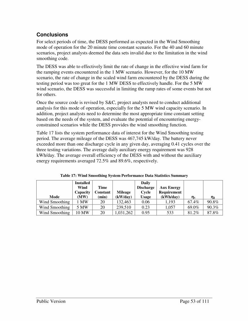
Public Version Page 53 of 111
Conclusions
For select periods of time, the DESS performed as expected in the Wind Smoothing mode of operation for the 20 minute time constant scenario. For the 40 and 60 minute scenarios, project analysts deemed the data sets invalid due to the limitation in the wind smoothing code.
The DESS was able to effectively limit the rate of change in the effective wind farm for the ramping events encountered in the 1 MW scenario. However, for the 10 MW scenario, the rate of change in the scaled wind farm encountered by the DESS during the testing period was too great for the 1 MW DESS to effectively handle. For the 5 MW wind scenario, the DESS was successful in limiting the ramp rates of some events but not for others.
Once the source code is revised by S&C, project analysts need to conduct additional analysis for this mode of operation, especially for the 5 MW wind capacity scenario. In addition, project analysts need to determine the most appropriate time constant setting based on the needs of the system, and evaluate the potential of encountering energy-constrained scenarios while the DESS provides the wind smoothing function.
Table 17 lists the system performance data of interest for the Wind Smoothing testing period. The average mileage of the DESS was 467,745 kW/day. The battery never exceeded more than one discharge cycle in any given day, averaging 0.41 cycles over the three testing variations. The average daily auxiliary energy requirement was 928 kWh/day. The average overall efficiency of the DESS with and without the auxiliary energy requirements averaged 72.5% and 89.6%, respectively.
Table 17: Wind Smoothing System Performance Data Statistics Summary
Mode
Installed
Wind
Capacity
(MW)
Time
Constant
(min)
Mileage
(kW/day)
Daily
Discharge
Cycle
Usage
Aux Energy
Requirement
(kWh/day) η1 η2
Wind Smoothing 1 MW 20 132,463 0.06 1,193 67.4% 90.8%
Wind Smoothing 5 MW 20 239,510 0.23 1,057 69.0% 90.3%
Wind Smoothing 10 MW 20 1,031,262 0.95 533 81.2% 87.8%

Public Version Page 54 of 111
Table 18: Effective Wind and Total Ramping Statistics for all Ramping Periods
Effective Wind Total
ID Start Time
(CT) End Time
(CT) Duration
(min) Direction Initial
kW Final kW
Delta kW
Avg Slope
(kW/min)
Max Slope
(kW/min) Initial
kW Final kW
Delta kW
Avg Slope
(kW/min)
Max Slope
(kW/min)
1 2/15/10 17:05
2/15/10 17:40 35 down -991 -645 346 10 23 -722 -745 -23 1 3
2 2/15/10 17:45
2/15/10 18:20 35 up -697 -986 -289 8 18 -730 -743 -13 0 4
3 2/15/10 21:40
2/15/10 22:40 60 down -883 -554 330 5 20 -816 -789 28 0 7
4 2/16/10 5:25 2/16/10 6:35 70 up -215 -647 -431 6 20 -237 -261 -23 0 3
5 1/31/10 20:00
1/31/10 20:30 30 up -164 -1028 -863 29 56 -330 -377 -46 2 24
6 1/31/10 22:20
1/31/10 22:50 30 up -457 -2573 -2116 71 119 -232 -1374 -1142 38 87
7 1/31/10 23:00
1/31/10 23:35 35 down -2256 -955 1301 37 76 -1401 -1277 124 4 18
8 2/1/10 4:35 2/1/10 5:50 75 up -1805 -4751 -2946 39 134 -1843 -3800 -1957 26 78
9 2/1/10 6:50 2/1/10 7:10 20 down -4074 -3099 975 49 126 -4097 -3747 350 17 32
10 2/1/10 7:10 2/1/10 7:30 20 up -3099 -4128 -1028 51 64 -3747 -3755 -7 0 13
11 2/1/10 9:15 2/1/10 9:35 20 down -3440 -1959 1481 74 107 -3206 -2909 297 15 30
12 2/1/10 9:35 2/1/10 9:55 20 up -1959 -2837 -877 44 94 -2909 -2749 161 8 13
13 1/22/10 13:20
1/22/10 14:25 65 up -2920 -6827 -3907 60 181 -2837 -5658 -2821 43 114
14 1/22/10 17:15
1/22/10 17:35 20 down -7274 -2475 4799 240 370 -7309 -3616 3693 185 332
15 1/22/10 17:40
1/22/10 17:55 15 up -2671 -8498 -5827 388 643 -3770 -7299 -3529 235 411
16 1/22/10 17:55
1/22/10 18:05 10 down -8498 -2679 5820 582 578 -7299 -3778 3522 352 349
17 1/22/10 18:15
1/22/10 19:25 70 up -5527 -8460 -2933 42 327 -4529 -7255 -2726 39 196
18 1/23/10 10:20
1/23/10 12:15 115 down -8551 18 8569 75 286 -8698 -1081 7617 66 286
19 1/23/10 16:15
1/23/10 17:30 75 up -133 -2218 -2084 28 150 18 -1494 -1511 20 72
20 1/23/10 17:35
1/23/10 18:20 45 up -1783 -5496 -3713 83 187 -1548 -4295 -2747 61 147
21 1/23/10 18:20
1/23/10 18:30 10 down -5496 -3008 2487 249 258 -4295 -3792 502 50 49
22 1/23/10 18:30
1/23/10 20:00 90 up -3008 -9801 -6793 75 348 -3792 -8601 -4809 53 251

Public Version Page 55 of 111
Effective Wind Total
ID Start Time
(CT) End Time
(CT) Duration
(min) Direction Initial
kW Final kW
Delta kW
Avg Slope
(kW/min)
Max Slope
(kW/min) Initial
kW Final kW
Delta kW
Avg Slope
(kW/min)
Max Slope
(kW/min)
23 1/24/10 1:15 1/24/10 2:30 75 down -8856 -3304 5552 74 263 -9154 -4404 4750 63 250
24 1/24/10 2:40 1/24/10 3:45 65 up -3431 -9335 -5904 91 268 -4530 -8136 -3606 55 202
25 1/24/10 5:50 1/24/10 8:40 170 down -9531 -2067 7464 44 205 -9328 -2320 7008 41 192
26 1/24/10 8:40 1/24/10 9:35 55 up -2067 -5624 -3557 65 188 -2320 -4455 -2135 39 173
27 1/24/10 10:25
1/24/10 11:20 55 up -5740 -9768 -4029 73 223 -5543 -8598 -3056 56 155
Table 19: DESS Ramping Statistics for all Ramping Periods
DESS
ID Start Time
(CT) End Time
(CT) Duration
(min) Direction Initial
kW Final kW
Delta kW
Avg Slope
(kW/min)
Max Slope
(kW/min) Delta SOC
Scaling Factor
Time Constant
(min) Correlation
1 2/15/10 17:05
2/15/10 17:40 35 Down 269 -100 -369 11 24 0.40% 8.7% 20 -0.05
2 2/15/10 17:45
2/15/10 18:20 35 Up -33 243 276 8 18 0.60% 8.7% 20 0.21
3 2/15/10 21:40
2/15/10 22:40 60 Down 67 -235 -302 5 19 -0.60% 8.7% 20 0.33
4 2/16/10 5:25 2/16/10 6:35 70 Up -22 386 408 6 20 2.20% 8.7% 20 0.64
5 1/31/10 20:00
1/31/10 20:30 30 Up -166 651 817 27 42 0.80% 43.3% 20 0.43
6 1/31/10 22:20
1/31/10 22:50 30 Up 225 1199 974 32 59 4.10% 43.3% 20 0.95
7 1/31/10 23:00
1/31/10 23:35 35 Down 855 -322 -1177 34 79 0.30% 43.3% 20 0.53
8 2/1/10 4:35 2/1/10 5:50 75 Up -38 951 989 13 76 9.60% 43.3% 20 0.94
9 2/1/10 6:50 2/1/10 7:10 20 Down -23 -648 -625 31 107 -2.00% 43.3% 20 0.50
10 2/1/10 7:10 2/1/10 7:30 20 Up -648 373 1021 51 61 -0.30% 43.3% 20 0.11
11 2/1/10 9:15 2/1/10 9:35 20 Down 234 -950 -1184 59 95 -1.30% 43.3% 20 0.80
12 2/1/10 9:35 2/1/10 9:55 20 Up -950 88 1038 52 107 -1.10% 43.3% 20 -0.71
13 1/22/10 13:20
1/22/10 14:25 65 Up 83 1169 1086 17 112 12.20% 86.6% 20 0.97
14 1/22/10 17:15
1/22/10 17:35 20 Down -35 -1141 -1106 55 80 -4.30% 86.6% 20 0.98
15 1/22/10 17:40
1/22/10 17:55 15 Up -1099 1199 2298 153 233 -1.00% 86.6% 20 0.92
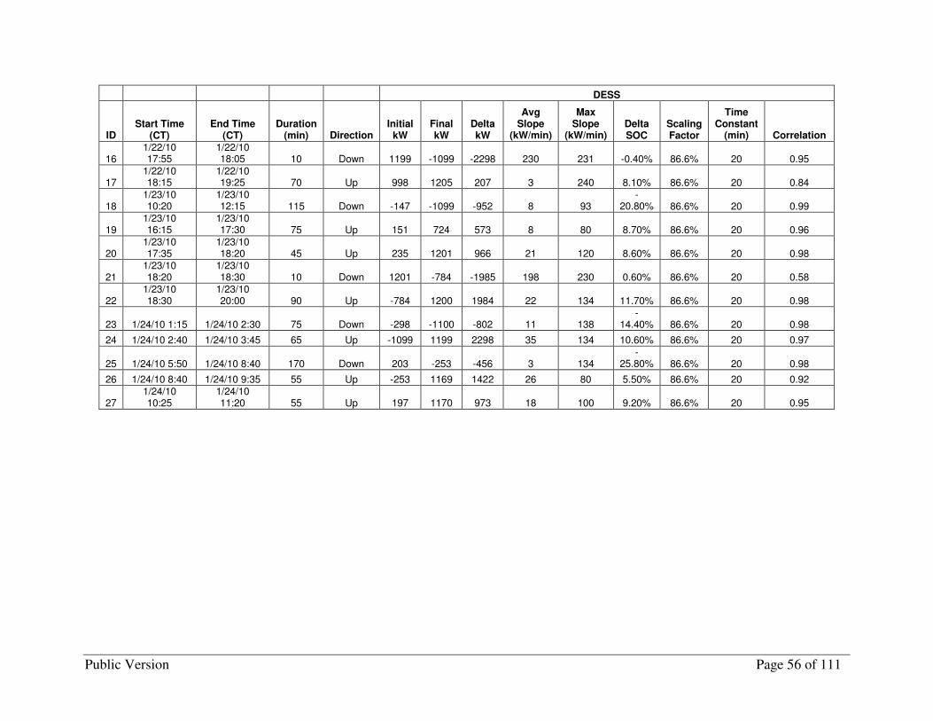
Public Version Page 56 of 111
DESS
ID Start Time
(CT) End Time
(CT) Duration
(min) Direction Initial
kW Final kW
Delta kW
Avg Slope
(kW/min)
Max Slope
(kW/min) Delta SOC
Scaling Factor
Time Constant
(min) Correlation
16 1/22/10 17:55
1/22/10 18:05 10 Down 1199 -1099 -2298 230 231 -0.40% 86.6% 20 0.95
17 1/22/10 18:15
1/22/10 19:25 70 Up 998 1205 207 3 240 8.10% 86.6% 20 0.84
18 1/23/10 10:20
1/23/10 12:15 115 Down -147 -1099 -952 8 93
-20.80% 86.6% 20 0.99
19 1/23/10 16:15
1/23/10 17:30 75 Up 151 724 573 8 80 8.70% 86.6% 20 0.96
20 1/23/10 17:35
1/23/10 18:20 45 Up 235 1201 966 21 120 8.60% 86.6% 20 0.98
21 1/23/10 18:20
1/23/10 18:30 10 Down 1201 -784 -1985 198 230 0.60% 86.6% 20 0.58
22 1/23/10 18:30
1/23/10 20:00 90 Up -784 1200 1984 22 134 11.70% 86.6% 20 0.98
23 1/24/10 1:15 1/24/10 2:30 75 Down -298 -1100 -802 11 138 -
14.40% 86.6% 20 0.98
24 1/24/10 2:40 1/24/10 3:45 65 Up -1099 1199 2298 35 134 10.60% 86.6% 20 0.97
25 1/24/10 5:50 1/24/10 8:40 170 Down 203 -253 -456 3 134 -
25.80% 86.6% 20 0.98
26 1/24/10 8:40 1/24/10 9:35 55 Up -253 1169 1422 26 80 5.50% 86.6% 20 0.92
27 1/24/10 10:25
1/24/10 11:20 55 Up 197 1170 973 18 100 9.20% 86.6% 20 0.95

Public Version Page 57 of 111
Dispatched Wind Leveling
Introduction
One of the value propositions in the W2B Test Plan is to evaluate the ability of large-scale battery storage technology to reduce the uncertainty of a variable generation resource. In the Wind Leveling mode, the DESS was used to hedge against error in the power forecast for the effective wind farm, thereby minimizing the impacts of uncertainty on the system. During this mode, the storage device varied its charging and discharging operations to minimize the difference between the expected and actual power output for the wind facility. Project participants tested this mode for each installed wind capacity scenario using a persistence forecast26.
Theory
Similar to conventional generators, wind facility operators, as MPs in the MISO market, must schedule the energy output from their facility with system operators. A MP has the option of scheduling the forecasted output of their wind facility in either the DA or RT market. Xcel Energy submits their wind into the DA market; and like all DA participants, Xcel Energy must submit their DA bids no later than 10:00 AM (CST) for the next operating day. Thus, when bidding wind in the DA market, MPs must forecast their wind output up to 38 hours in advance. As already confirmed by several studies, wind speeds and power forecast errors increase with forecast lead time [Ortech Power, NERC]. The benefit of using energy storage for wind leveling, therefore, becomes more valuable for longer forecast horizons.
Additionally, as discussed in the Economic Dispatch section, if the forecasted amount of wind energy deviates from the actual amount, the MP is forced to true up their position in the RT market. Although this true up process may or may not be at uneconomical prices, there is a large degree of uncertainty in the process and that uncertainty exposes the MP to market risk.
Furthermore, although renewable generation resources are not currently susceptible to RSG charges, MISO may alter their energy tariff in the future to start assigning these charges to wind facility operators for activity in the RT market. Therefore, in the future, it may become more important for a MP to have an accurate wind energy forecast for market settlement purposes.
For the Wind Leveling mode of the DESS, a user specifies the desired power output value for the effective wind farm. As the actual power output from the scaled farm deviates from the desired (i.e. scheduled) value, logic residing on the PCS commands the battery to charge and discharge to compensate for the difference. For example, if the forecast under-predicts the actual output of the scaled wind farm, the DESS will charge at a rate that minimizes the scheduling error. Likewise, if the forecast over-predicts the actual output of the scaled wind farm, the DESS will discharge at a rate that minimizes the scheduling error.
While in this mode, the user monitors the output of the MWD site in real-time. In the event of significant deviations between the scheduled and actual values, the user will update the desired power set-point to minimize the mismatch and conserve battery operation. Ideally, over time, the amount of energy over-forecasted will be approximate to the amount of energy under-forecasted,
26 Herein, persistence forecasting refers to using current power output to forecast future output.
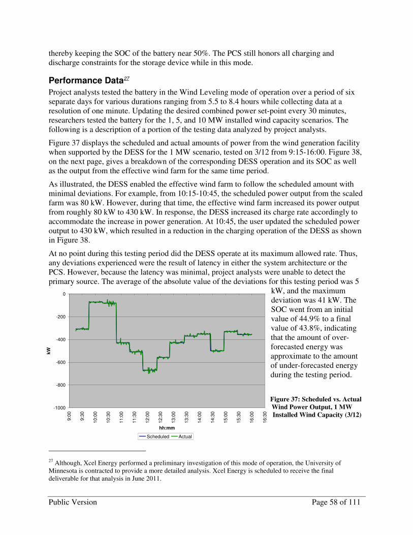
Public Version Page 58 of 111
-1000
-800
-600
-400
-200
0
9:0
0
9:3
0
10:0
0
10:3
0
11:0
0
11:3
0
12:0
0
12:3
0
13:0
0
13:3
0
14:0
0
14:3
0
15:0
0
15:3
0
16:0
0
16:3
0
hh:mm
kW
Scheduled Actual
thereby keeping the SOC of the battery near 50%. The PCS still honors all charging and discharge constraints for the storage device while in this mode.
Performance Data27
Project analysts tested the battery in the Wind Leveling mode of operation over a period of six separate days for various durations ranging from 5.5 to 8.4 hours while collecting data at a resolution of one minute. Updating the desired combined power set-point every 30 minutes, researchers tested the battery for the 1, 5, and 10 MW installed wind capacity scenarios. The following is a description of a portion of the testing data analyzed by project analysts.
Figure 37 displays the scheduled and actual amounts of power from the wind generation facility when supported by the DESS for the 1 MW scenario, tested on 3/12 from 9:15-16:00. Figure 38, on the next page, gives a breakdown of the corresponding DESS operation and its SOC as well as the output from the effective wind farm for the same time period.
As illustrated, the DESS enabled the effective wind farm to follow the scheduled amount with minimal deviations. For example, from 10:15-10:45, the scheduled power output from the scaled farm was 80 kW. However, during that time, the effective wind farm increased its power output from roughly 80 kW to 430 kW. In response, the DESS increased its charge rate accordingly to accommodate the increase in power generation. At 10:45, the user updated the scheduled power output to 430 kW, which resulted in a reduction in the charging operation of the DESS as shown in Figure 38.
At no point during this testing period did the DESS operate at its maximum allowed rate. Thus, any deviations experienced were the result of latency in either the system architecture or the PCS. However, because the latency was minimal, project analysts were unable to detect the primary source. The average of the absolute value of the deviations for this testing period was 5
kW, and the maximum deviation was 41 kW. The SOC went from an initial value of 44.9% to a final value of 43.8%, indicating that the amount of over-forecasted energy was approximate to the amount of under-forecasted energy during the testing period.
Figure 37: Scheduled vs. Actual
Wind Power Output, 1 MW
Installed Wind Capacity (3/12)
27 Although, Xcel Energy performed a preliminary investigation of this mode of operation, the University of Minnesota is contracted to provide a more detailed analysis. Xcel Energy is scheduled to receive the final deliverable for that analysis in June 2011.

Public Version Page 59 of 111
-4400
-4000
-3600
-3200
-2800
-2400
-2000
-1600
-1200
-800
-400
0
13
:00
13
:30
14
:00
14
:30
15
:00
15
:30
16
:00
16
:30
17
:00
17
:30
18
:00
18
:30
19
:00
hh:mm
kW
Scheduled Actual
-1000
-750
-500
-250
0
250
500
750
1000
9:0
0
9:3
0
10:0
0
10:3
0
11:0
0
11:3
0
12:0
0
12:3
0
13:0
0
13:3
0
14:0
0
14:3
0
15:0
0
15:3
0
16:0
0
16:3
0
hh:mm
kW
0%
20%
40%
60%
80%
100%
SO
C
DESS (kW) Effective Wind (kW) SOC (%)
Figure 38: DESS, Effective Wind, and SOC, 1 MW Installed Wind Capacity (3/12)
Figure 39 and Figure 40 display the same data series for the 5 MW scenario analysts tested on 3/9 from 13:00-19:00. Similar to before, the actual output closely followed the scheduled amount with assistance from the DESS. Unlike the 1 MW scenario, the DESS operated at its maximum rates while trying to minimize the mismatches between the scheduled amount and actual amount. However, the DESS was still able to continue having the effective wind farm follow its scheduled output. For this test, the average of the absolute value of deviations was 22 kW, and the maximum deviation was 323 kW. The SOC decreased 5.2% as it went from 50.1% to 44.9%, indicating that there was a slight bias in over-forecasting the power output from the scaled wind farm during the testing period.
Figure 39: Scheduled vs. Actual Wind Power Output, 5 MW Installed Wind Capacity (3/9)
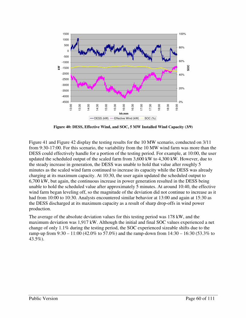
Public Version Page 60 of 111
-4500
-4000
-3500
-3000
-2500
-2000
-1500
-1000
-500
0
500
1000
1500
13
:00
13
:30
14
:00
14
:30
15
:00
15
:30
16
:00
16
:30
17
:00
17
:30
18
:00
18
:30
19
:00
hh:mm
kW
0%
20%
40%
60%
80%
100%
SO
C
DESS (kW) Effective Wind (kW) SOC (%)
Figure 40: DESS, Effective Wind, and SOC, 5 MW Installed Wind Capacity (3/9)
Figure 41 and Figure 42 display the testing results for the 10 MW scenario, conducted on 3/11 from 9:30-17:00. For this scenario, the variability from the 10 MW wind farm was more than the DESS could effectively handle for a portion of the testing period. For example, at 10:00, the user updated the scheduled output of the scaled farm from 3,600 kW to 4,300 kW. However, due to the steady increase in generation, the DESS was unable to hold that value after roughly 5 minutes as the scaled wind farm continued to increase its capacity while the DESS was already charging at its maximum capacity. At 10:30, the user again updated the scheduled output to 6,700 kW, but again, the continuous increase in power generation resulted in the DESS being unable to hold the scheduled value after approximately 5 minutes. At around 10:40, the effective wind farm began leveling off, so the magnitude of the deviation did not continue to increase as it had from 10:00 to 10:30. Analysts encountered similar behavior at 13:00 and again at 15:30 as the DESS discharged at its maximum capacity as a result of sharp drop-offs in wind power production.
The average of the absolute deviation values for this testing period was 178 kW, and the maximum deviation was 1,917 kW. Although the initial and final SOC values experienced a net change of only 1.1% during the testing period, the SOC experienced sizeable shifts due to the ramp-up from 9:30 – 11:00 (42.0% to 57.0%) and the ramp-down from 14:30 – 16:30 (53.3% to 43.5%).
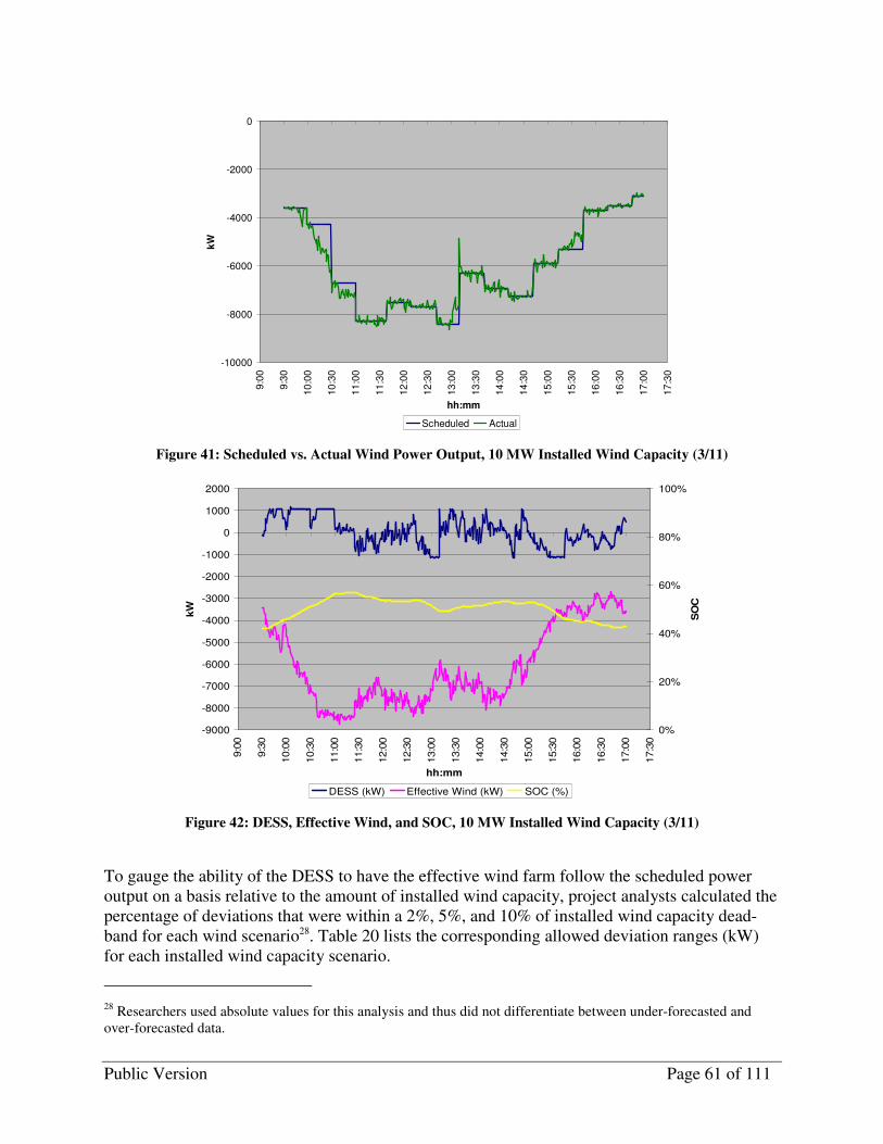
Public Version Page 61 of 111
-10000
-8000
-6000
-4000
-2000
0
9:0
0
9:3
0
10
:00
10
:30
11
:00
11
:30
12
:00
12
:30
13
:00
13
:30
14
:00
14
:30
15
:00
15
:30
16
:00
16
:30
17
:00
17
:30
hh:mm
kW
Scheduled Actual
Figure 41: Scheduled vs. Actual Wind Power Output, 10 MW Installed Wind Capacity (3/11)
-9000
-8000
-7000
-6000
-5000
-4000
-3000
-2000
-1000
0
1000
2000
9:0
0
9:3
0
10:0
0
10:3
0
11:0
0
11:3
0
12:0
0
12:3
0
13:0
0
13:3
0
14:0
0
14:3
0
15:0
0
15:3
0
16:0
0
16:3
0
17:0
0
17:3
0
hh:mm
kW
0%
20%
40%
60%
80%
100%
SO
C
DESS (kW) Effective Wind (kW) SOC (%)
Figure 42: DESS, Effective Wind, and SOC, 10 MW Installed Wind Capacity (3/11)
To gauge the ability of the DESS to have the effective wind farm follow the scheduled power output on a basis relative to the amount of installed wind capacity, project analysts calculated the percentage of deviations that were within a 2%, 5%, and 10% of installed wind capacity dead-band for each wind scenario28. Table 20 lists the corresponding allowed deviation ranges (kW) for each installed wind capacity scenario.
28 Researchers used absolute values for this analysis and thus did not differentiate between under-forecasted and over-forecasted data.

Public Version Page 62 of 111
For example, if in the 1 MW wind scenario there was a deviation with an absolute value of 75 kW, the DESS would have been successful for the 10% criterion but not for the 2% or 5% cases since it exceeded the corresponding maximum allowed absolute values (20, 50 kW). As another example, if in the 10 MW scenario there was a deviation with an absolute value of 175 kW, the DESS would have been successful for all three cases (i.e., 2%, 5%, and 10%).
Figure 43 displays the results of this analysis for each of the six testing periods. Because of the larger allowed deviation range for the higher wind capacity scenarios, the results from the various wind scenarios were similar (sans the 3/11 testing date). At a 2% tolerance, at least 96% of the deviations for the 1 MW and 5 MW scenarios fell within the allowed range for the testing data collected. For the 10 MW scenario, the results varied significantly (97.2% and 76.3%), thus making it difficult to draw any conclusive results.
Table 20: Relative Allowed Deviations in Scheduled vs.
Actual Wind Power as a Function of Wind Capacity
Allowed Deviation Range (±kW)
Allowed Deviation
Percentage
Installed Wind Capacity (MW) 2% 5% 10%
1 20 50 100
5 100 250 500
10 200 500 1,000
0%
10%
20%
30%
40%
50%
60%
70%
80%
90%
100%
3/12 2/23 3/9 2/25 3/10 3/11
1 MW 5 MW 10 MW
Installed Wind Capacity
% o
f T
ime W
ith
in A
llo
wed
Dead
-Ba
nd
.
2% 5% 10%
Figure 43: Percentage of Deviations within Allowed Range

Public Version Page 63 of 111
Conclusions
Overall, the DESS performed well for the 1 MW and 5 MW testing periods. The results for the 10 MW scenario varied too much, preventing analysts from drawing any detailed insights. For all the scenarios, the DESS performed as expected, responding to changes in the output from the effective wind farm rapidly and accurately. The 1 MW DESS is effectively capable of leveling 1 MW of installed wind capacity. However, additional testing data is required for the 5 MW and 10 MW scenarios to better determine the leveling capability of the DESS for a more statistically valid set of wind profiles. In addition, project analysts should conduct additional testing for this mode, substituting forecasted values from the company’s various wind forecasting programs for the scheduled output value and then evaluate the difference in results compared to the persistence methodology.
Table 21 lists the system performance data of interest for the Wind Leveling testing period. The average mileage of the DESS was 125,360 kW/day. The battery never exceeded more than one discharge cycle in any given day, averaging 0.56 cycles over the three testing variations. The average daily auxiliary energy requirement was 834 kWh/day. The average overall efficiency of the DESS with and without the auxiliary energy requirements averaged 67.6% and 91.6%, respectively.
Table 21: Wind Leveling System Performance Data Statistics Summary
Mode
Installed
Wind
Capacity
(MW)
Mileage
(kW/day)
Daily
Discharge
Cycle
Usage
Aux Energy
Requirement
(kWh/day) η1 η2
Wind Leveling 1 MW 34567 0.32 1230 44.2% 95.8%
Wind Leveling 5 MW 145723 0.54 344 83.3% 90.2%
Wind Leveling 10 MW 195791 0.82 929 75.3% 88.8%
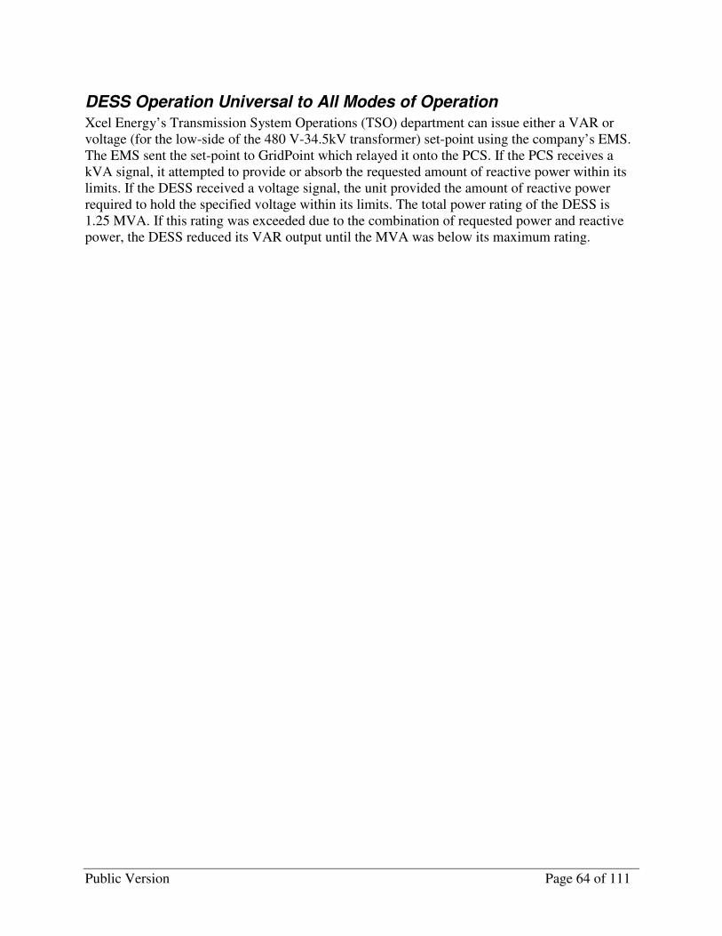
Public Version Page 64 of 111
DESS Operation Universal to All Modes of Operation
Xcel Energy’s Transmission System Operations (TSO) department can issue either a VAR or voltage (for the low-side of the 480 V-34.5kV transformer) set-point using the company’s EMS. The EMS sent the set-point to GridPoint which relayed it onto the PCS. If the PCS receives a kVA signal, it attempted to provide or absorb the requested amount of reactive power within its limits. If the DESS received a voltage signal, the unit provided the amount of reactive power required to hold the specified voltage within its limits. The total power rating of the DESS is 1.25 MVA. If this rating was exceeded due to the combination of requested power and reactive power, the DESS reduced its VAR output until the MVA was below its maximum rating.

Public Version Page 65 of 111
General Conclusions and Lessons Learned The previous sections have provided insights and conclusions related to specific modes of operation. The following is a list of the general conclusions related to the DESS as a whole, based on the tests conducted to date and the related testing conditions:
� The overall efficiency of the DESS, accounting for the auxiliary energy requirements, displayed considerable variation as a function of mode of operation, ranging from 67.6% to 78.9%.
� The efficiency of the DESS, not accounting for the auxiliary energy requirements, displayed less variation as a function of mode of operation, ranging from 85.1% to 91.6%.
� The DESS never exceeded more than one discharge cycle in any 24-hour period for any mode of operation.
� The DESS mileage varied significantly depending on the mode of operation. Based on the mileage metric, the Frequency Regulation mode of operation was the most aggressive mode while the Economic Dispatch mode was the least aggressive.
In addition, project analysts took a few moments to look back and answer the question “What should we have done differently?” Below are those observations as related to the system architecture, analytics, project siting and other lessons learned.
System Architecture
� When working with multiple data systems that interact with one another to varying degrees, it is critical to ensure that the method of connectivity between any two systems is compatible and within the original scope of work.
In regards to interfacing with a remote operator, S&C stated in their specification that the
PCS was capable of supporting either the Distributed Network Protocol 3.0 (DNP3) or
Modbus Plus (MB+) protocols for the SCADA interface. However, this requirement was not
accounted for when Xcel Energy was in contract negotiations with GridPoint to provide their
services to the project. Several months into the project, the communication team realized that
the protocol GridPoint was planning on using to communicate with the PCS was not
compatible with the PCS. As a result, GridPoint had to submit a change order request to
Xcel Energy to revise its original plan and enable GridPoint to incorporate the DNP3
protocol into their servers. This added to the cost of the project and extended the project
schedule by approximately 6 weeks.
� A first-of-a-kind control system covering multiple modes of operation spans a wide array of skill sets and requires an extensive amount of development time.
Project participants required an extensive amount of time to define in detail the various
modes of operation, which required multiple iterations to the PCS specification and control
set-points list. Consequently, S&C was delayed in beginning their required programming
tasks. Although the first iteration of the points list was issued in August of ’08, the final
version of the PCS specification was not completed until March ’09. However, due to project
management constraints, the PCS was shipped and installed in November 2008. Although
some work on the communication system was done in parallel to work on the modes of

Public Version Page 66 of 111
operation, the communication team was dependent on several of the functional requirements
outlined by the operation modes. Thus, work on the communication system was also delayed.
� Once designed, a first-of-a-kind control system also requires an extensive amount of programming time and a thorough commissioning process.
After the design specification and control set-points list was finalized, S&C started to
program the PCS, originally scheduling one month to complete the task. To minimize the
amount of errors encountered in the field, since the PCS had already been installed, S&C
constructed a control test-bed and S&C and GridPoint performed lab-to-lab testing over the
course of several weeks to ensure data connectivity between the two systems. S&C also
performed in-house testing of the software to minimize errors in the control logic29. After the
completion of these tasks, S&C installed the W2B software on the PCS at the project site in
April 2010.
To verify the PCS operated according to the specification, Xcel Energy generated a field
commissioning document30. During the field testing procedures, project analysts encountered
multiple errors that were not originally identified during the lab testing without the PCS. To
account for these errors, S&C responded by implementing an updated version of the software
in July 2009. However, over the course of several months that followed, project analysts
continued to find additional errors in the control logic as they explored each mode of
operation in greater detail. Xcel Energy is working with S&C on correcting the identified
errors and plans on uploading the newest software version in Q3 2010.
� Smart grid applications such as the W2B Project and others are changing the traditional utility IT paradigm in that network based equipment is now starting to make its presence out in the field. Therefore, it is important to develop a long-term strategy that outlines a formal procedure for installing and maintaining these types of devices in their new operating environments.
As mentioned in the description of some of the interfaces, the W2B communication team
implemented Ruggedcom devices throughout the design of the system to enable the different
components to communicate with one another. A RX1000 router, RS910 switch, and RS900
switch were installed at the Luverne site.
Prior to the project, Xcel Energy’s Communication Infrastructure department was not
familiar with these devices because Xcel Energy’s preferred IT platform is CISCO. As a
result, the department initially did not agree to assist with installing and supporting these
devices. However, after discussing the matter, the Communication Infrastructure department
agreed that the decision to go with Ruggedcom devices was appropriate for the given
application.
Ultimately, engineers from Xcel Energy’s Substation Engineering Design department
installed the Ruggedcom devices at the site after working closely with support engineers from
Ruggedcom over several days. However, ongoing support of the devices is still problematic
in that the engineers familiar with theses devices are located in Minneapolis.
29 S&C Electric Company. “Wind to Battery Software Factory Test Procedure (Version 4).
30 Xcel Energy. “Wind-to-Battery Field Commissioning Testing”.

Public Version Page 67 of 111
� In order to utilize the full charge-discharge range of the battery (i.e. a swing from +1MW to -1MW and vice versa) when providing frequency regulation, the AGC system must be capable of issuing both positive and negative MW commands.
During the design of the W2B communication system, the team realized that Xcel Energy’s
NSP EMS system could only send out a positive MW command to units on AGC control.
Thus, the battery would have been unable to provide regulation both as a generator and as a
load. As a result, the project team contacted Siemens, Xcel Energy’s EMS provider, to
determine the required programming changes that would enable the AGC system to issue
both positive and negative MW commands. Because it was important to project sponsors to
show the battery capable of providing frequency regulation both when it was charging and
discharging, a Statement of Work between Xcel Energy and Siemens was drafted to perform
the required code changes. After initial lab testing and field testing with the battery, the
updated AGC code was successfully implemented in June 2009, approximately one month
after its expected availability date. In addition to the month delay, the modification added to
the project cost.
� Other lessons learned from the W2B project related to the communications and control architecture include the following:
o Include in the points list a nominal maximum charge and discharge rate and an emergency charge and discharge capacity rate;
o For each analog output set-point specify an allowed input range, data type, resolution, sign convention, scaling, and a master;
o When implementing a control points list, be sure to include a read or “echo” on all analog outputs to verify that the correct value for each set-point has been issued;
o When implementing a control points list, map all analog outputs to inputs so that a user can verify whether the unit has received and successfully administered the requests;
o Provide whatever department that will be responsible for responding to system alarms with the desired level of detail on system status information;
o The power electronics associated with an electrochemical storage device should include a generator droop response functionality to automatically respond to perturbations in grid frequency31;
o Before a loss of communication alarm is issued, it first shall exceed a minimum time duration.
� As for the PCS control logic, project analysts have identified potential modifications for some of the modes of operation that could enhance their respective value.
o While testing the Wind Smoothing mode, project researchers identified multiple periods in which the DESS was used to smooth volatility that was unlikely to result in difficulty for system operators. Thus, project researchers may want to work closely with S&C engineers to investigate other smoothing logic that still has the storage device supporting the wind facility during critical ramping events but remains idle during periods of
31 Currently, the DESS maintains a constant power output regardless of changes in grid frequency.

Public Version Page 68 of 111
temperate volatility. This modification would minimize battery operation and extend system life.
o For the Wind Leveling mode, project researchers recommend that an allowed dead-band be placed around the desired target level so that the DESS only operates when the absolute value of the deviations exceed a certain threshold. Again, because the grid can handle a certain amount of uncertainty (i.e. noise) in power output from any type of generating facility, there is not a strong system need to have a generator exactly follow its generation scheduled. By implementing this feature, DESS operation will be reserved for more critical times, thereby minimizing battery operation and extending system life. Furthermore, the control logic should be able to accept a schedule for a given forecast horizon and resolution that a user can specify upfront. This modification will avoid the limitation of requiring the user to manually update the set-point.
Analytics
� When defining a project test plan, researchers shall identify only the most appropriate and/or effective analytics approach for each value proposition in order to establish a plan that is reasonable in scope and yet extensive enough to cover important research areas.
Xcel Energy worked with internal and external analysts and researchers to identify multiple
value propositions that warranted investigation for the W2B Project. While all the
propositions were valid and justified, together they covered an expansive range of research
topics concerning storage and wind energy. As a result, it was difficult for project
researchers to identify the most appropriate and/or effective analytics approach for each
value proposition.
Furthermore, once project researchers identified a method of analysis and began collecting
data, it was readily apparent that additional time was required for the data gathering and
analysis phase of the project to adequately cover each value proposition. In addition to the
multiple modes of operation, project researchers encountered multiple errors in the datasets
due to variety of reasons ranging from user input error, communication outages, and
unexpected PCS operation. Regardless of the cause, each invalid dataset required project
researchers to retest the battery, resulting in greater time requirements.
� Establish a central on-site data repository that collects data from all the appropriate sources with uniform time stamps.
For the W2B Project, GridPoint used the DNP3 protocol to collect and archive data, which
project researchers then used in their analysis. However, because DNP3 is a polling
protocol and can not simultaneously access two separate device, analysts were unable to
work with time -synchronized data whenever they had to access two separate data sources.
Because the difference in time stamps was only a few seconds, the impacts on data analysis
was minimal. However, the impact on the project researchers’ ability to troubleshoot the
system was much greater.
� Conduct analyses on both simulated and empirical data.
For the wind-coupled modes (i.e., Basic GS, Wind Smoothing, and Wind Leveling), testing
was dependent on the output of the scaled wind farm, which was never identical for any two
given testing periods. Thus, it was difficult for project analysts to directly compare results

Public Version Page 69 of 111
from one day to another due to non-uniform testing conditions. One way in which project
analysts can get around this limitation is by conducting a similar analysis on simulated data
rather than just empirical data. NREL has developed a model of the NaS battery that will
enable Xcel Energy and other project participants to carry out this type of analysis if there is
sufficient interest and resources.
� Other lessons learned from the W2B project related to analytics include the following:
o If possible, explicitly measure the energy embedded in output of the effective wind farm;
o On the user interface page for the Economic Dispatch mode, include information on the current price bin, SOC bin, and what market mode the DESS is operating under;
o Highly accurate efficiency measurements of systems of this nature require extremely precise instrumentation.
Project Siting and Logistics
� Although locating the battery next to a wind farm provided many benefits, the rural location of the project site introduced multiple logistical issues for project participants.
Luverne, MN is approximately a four hour drive from Minneapolis, MN, which is where Xcel
Energy’s Substation Design and Construction Department is located. This was the primary
department involved in the installation and commissioning of the communication and control
equipment for Xcel Energy. Due to the extended drive between the two locations, it was
difficult to schedule time for Xcel Energy engineers to head out to the W2B site for the initial
installation as well as to return to the site throughout the project whenever troubleshooting
was required.
In addition, because of the remoteness of the location, Xcel Energy had difficulty agreeing
upon an internal department that would provide on-site support. Ultimately, Xcel Energy’s
Angus Anson plant accepted this responsibility; however, being located in Sioux Falls, SD,
they are still approximately 30 minutes away from the site.
By locating the battery in a more central location, project participants expect to see a
reduction in down time during troubleshooting and more willingness from other internal
departments to accept ownership responsibilities.
Other Lessons Learned
� When working with a team that consists of multiple departments and outside vendors, it is critical to clearly define roles and responsibilities at the onset.
Because no single department or organization had all the required knowledge, the project
team consisted of multiple Xcel Energy departments and outside vendors. As a result, some of
the project participants were uncertain about roles and responsibilities for each of the
members, resulting in delay in the project schedule.
� When establishing long-term business arrangements with vendors, it is critical to establish fair but favorable business arrangements for the company that are mutually agreed upon and signed by both parties.
Xcel Energy originally selected V2Green to provide their Intelligent Distributed Generation
Solution to the W2B Project. Although the initial agreement was only for the first year of

Public Version Page 70 of 111
operation, the tacit agreement between directors at Xcel Energy and V2Green was that due
to the R&D nature of the project, in which both parties stood to benefit by acquiring
additional knowledge, V2Green would continue to offer its services to Xcel Energy at a
discounted rate.
However, in September 2008, GridPoint acquired V2Green, which brought in new GridPoint
directors for the Xcel Energy account. During negotiations regarding the extension of
GridPoint’s services to the project, Xcel Energy believed that the new GridPoint directors
did not acknowledge the nature of the original agreement when they submitted the proposal
for extending their services. As a result, Xcel Energy investigated alternative control and
data acquisition methods and decided to implement an in-house solution to replace
GridPoint. Consequently, the amount Xcel Energy paid GridPoint only covered a service
period of a little over a year, excluding any additional charges for change order. In addition,
Xcel Energy had to spend additional funds to develop an in-house solution.
� When working with first-of-a-kind technology it is important to always account for both short-term and long-term ownership responsibilities.
For this project, there were two primary areas of ownership responsibility: 1) Activities
related to providing on-site support for ongoing O&M procedures for the NaS battery, the
PCS, and the communication system, and 2) Activities related to coordinating with Xcel
Energy’s TSO department and Minwind for system outages taken at the site.
To the extent possible, it is critical to identify the department(s) with this responsibility either
at the outset of the project or as soon as logistically possible. Because it determines what
alarms it wants to receive and how it goes about receiving said alarms, this department
needs to be included in the design and implementation of the system architecture.
Furthermore, project participants need to work with the on-site responders to categorize the
available alarms and define the appropriate responses for each type. Lastly, to avoid the risk
of serious injury or death to support personnel, the department with ownership
responsibilities needs to work with the TSO and other appropriate outside parties (i.e.
Minwind) to define the protocol that is to be followed when scheduling an outage at the site.

Public Version Page 71 of 111
Public Policy Considerations Great Plains Institute (GPI) has been working with Xcel Energy over the past year to assist in preparation of policy recommendations to support the potential expansion of electric energy storage on the Xcel Energy system if the results of this project and others indicate that energy storage is determined to be a valuable and effective tool to integrate intermittent renewable energy on the system. Xcel Energy and GPI convened a series of policy work group meetings and webinars to help provide input and advice on policy recommendations which would help support expansion of electric energy storage options. The main objective of the policy work group is outlined below.
Policy Work Group Approach and Process
Work Group Objective
Identify policy changes necessary to expand the deployment of electric energy storage and provide flexibility for application to generation, transmission or distribution systems.
A series of questions in each Policy Focus Areas was discussed with the policy work group in a series of meetings/webinars on September 23rd, 2009, December 16th, 2009 and April 13th, 2010 along with follow-up interviews with several individuals (subject matter experts).
These policy issues were divided into jurisdictional areas including the Federal Energy Regulatory Commission (FERC), MISO, State regulatory arena and utility policies to facilitate discussion and help clarify recommendations.
Key Assumptions For Analysis
Electric energy storage options such as Compressed Air Energy Storage (CAES), batteries, flywheels, and hydrogen energy storage are still in the development stage with limited operational experience except for several large scale pumped-storage hydro projects such as Ludington32. Several new demonstration projects using these technologies are being funded by DOE as part of their Smart Grid demonstration grants. As a result, operational and financial
32 The Ludington pumped storage facility on Lake Michigan, built in the early 1970s by Consumers Power and Detroit Edison, has over 1,800 MW of capacity. Because of its location, it is now being considered for its ability to load follow wind energy.
Policy Focus Areas: � What policy changes are needed in order to expand the
deployment of energy storage for generation, transmission or distribution system applications?
� What additional policy changes are needed in order to maximize
the [public] reliability benefits of energy storage for generation, transmission or distribution system applications?
� What additional policy changes are needed in order to maximize
the [public] economic benefits of energy storage for generation, transmission or distribution system applications?
� What additional policy changes are needed in order to maximize
the [public] environmental benefits of energy storage for generation, transmission or distribution system applications?

Public Version Page 72 of 111
regulations and policies are still in the early stages of development by FERC and regional transmission organizations such as MISO and PJM Interconnection.
The policy work group based their work on several key assumptions regarding the electrical grid and future generation options:
� Wind energy will continue to expand in the MISO footprint and will cause increasing system operating issues and transmission congestion issues for the MISO around wind integration, load following, cost of generation alternatives and value of quick-response electric energy storage options.
� There will be potential areas of economic value for electric energy storage including:
o Enhancing variable renewable generation by time shifting, curtailment avoidance, smoothing and ramp rate control.
o Reduced power plant cycling and availability requirements including spinning reserve value, Operating and Maintenance (O&M) savings, and avoided costs associated with turning down baseload generation to minimum operating levels where they are not designed to operate.
o Transmission and distribution grid systems support including ancillary services such as frequency regulation, wind curtailment avoidance, peak shaving and power quality.
o Hidden dispatch cost avoidance.
o Natural gas price hedge.
o Deferral of costs associated with transmission and distribution investments.
� Long-term environmental and regulatory benefits from carbon dioxide (CO2) regulations are difficult to quantify until federal requirements around CO2 reductions, taxes or cap and trade are completed and the additional value of storing renewable energy under those assumptions can be quantified.
Principles and Guidelines
The policy work group used the following principles and guidelines to work through the major policy questions and provide recommendations:
1. Policy should encourage optimizing storage investments in support of overall system efficiency and cost effectiveness.(Cost, reliability and environmental benefit)
2. Policy should generate the most good for the largest number of customers

Public Version Page 73 of 111
Policy Work Group Participants
Xcel Energy Frank Novachek, Project Sponsor Nancy Pellowski, Project Support Jim Himelic, Project Analyst Betsy Engelking, Resource Planning Lloyd Hilgard, Energy Supply Dan Pfeiffer, Government Affairs Liam Noailles, Market Operations Marty Smith, Environmental Policy Steve Beuning, Market Operations
External Participants Rolf Nordstrom, Great Plains Institute Mike Gregerson, Great Plains Institute Mark Willers, Minwind Energy LLC Matt Schuerger, Energy Systems Consulting Svs Rahul Walawalkar, Customized Energy Solutions Stan Selander, Great River Energy Harold Gotschall, Technology Insights Nathaniel Baer, Iowa Environmental Council Larry Johnston, SUMMPA Tom Wind, Iowa Stored Energy Park
Key Policy Considerations and Recommendations
The following summarizes key discussions and recommendations discussed by the work group for further consideration as policy development relevant to electric energy storage evolves.
FERC and MISO Policy Areas
1. There is no FERC approved tariff for electric energy storage in the MISO market
a. Discussion: Since the issuance of this recommendation, the MISO has submitted a proposed electric energy storage tariff to FERC, which was conditionally approved in an order on May 10th, 2010. Additional clarification was requested by FERC on some of the tariff language. This was completed on June 9th, 2010.
b. Recommendation: The W2B project will start to operate in July 2010 in the MISO market under the new electric energy storage tariff. Any further recommendations for changes to help support the expansion of electric energy storage in the MISO market will be supported by future operating experience and determination of benefits by Xcel Energy.
2. Electric energy storage may need to be considered a separate asset class to support expanded deployment
a. Discussion: Electric energy storage devices in most energy markets are not given any flexibility on asset classification or operating options to maximize the asset in the energy generation or transmission marketplace.
b. Recommendation: Allow longer term electric energy storage devices, which can operate 4 to 8 hours, to provide both energy delivery and frequency regulation services in the MISO market to maximize operating and revenue potential; and, consider the option of SERs to be paid for capacity services and bid into day ahead markets.

Public Version Page 74 of 111
3. There may be many different ways, depending on the timing, of how SER can provide services to the MISO market
a. Discussion: SERs, especially those owned by integrated utilities, should have the flexibility to provide multiple services as a generation, transmission and/or distribution asset, either simultaneously or as conditions change.
b. Recommendation: Allow SERs to be service providers for the generation, transmission and/or distribution portions of the electric utility without penalty or restriction.
4. Electric energy storage devices that use net energy for frequency regulation services are expected to pay retail rates for energy
a. Discussion: If SER devices can help with frequency regulation services, then they should not be penalized by paying retail rates for the electricity they use.
b. Recommendation: Allow SER to pay wholesale rates for energy use during frequency regulation services.
5. MISO does not do planning for assets below 5MW
a. Discussion: Unless SERs are aggregated, it will be difficult to get study results from MISO that can show the proper location and benefits for SER devices as transmission or generation assets.
b. Recommendation: Request MISO to make a special category of study for SER services with a minimum size, such as 5 MW, to be determined.
6. Quick response assets such as battery and flywheel SERs are not given special valuation by MISO beyond the normal spinning reserve payments given to conventional generation
a. Discussion: SERs can provide a valuable service with very quick, sometimes sub-minute, response services to MISO that would be valuable in certain locations and time periods.
b. Recommendation: Request that MISO and FERC look at a special valuation for SERs such as batteries and flywheels that can provide very quick response services.
Environmental/Reliability Policy Areas
1. Cost Allocation for regional transmission projects related to wind power development will help determine some valuations of electric energy storage in remote areas
a. Discussion: The MISO is completing the Regional Generator Outlet Study (RGOS) for the Midwest region, along with a new transmission cost allocation tariff to be submitted to FERC by July 15th, 2010.
b. Recommendation: Once new cost allocation tariffs are available for wind related transmission projects, determine a methodology for assessing the value of electric energy storage devices in terms of maximizing the use of wind energy resources on new transmission lines.
2. Greenhouse Gas (GHG) Valuation from a cap and trade regulation or a carbon tax will help determine environmental benefits of electric energy storage devices

Public Version Page 75 of 111
a. Discussion: Electric energy storage devices that can provide storage and peak period release of renewable energy can have valuations above those services to the normal energy market and enable more variable renewable resources on the grid.
b. Recommendation: Modeling should be conducted to determine minimum carbon price levels that would result in significant benefits to renewable electric energy storage.
Recent Policy Developments
Two new processes moved forward in FERC and the MISO recently that were deemed by the policy work group to be important for the future successful expansion of electric energy storage devices within the MISO system.
1. FERC Order on MISO Stored Energy Resources Tariff:
As noted in the discussion above (FERC and MISO policy recommendation #1), FERC issued a conditional order accepting MISO’s Stored Resource Compliance Filing under Docket No. ER07-1372-017 and ER09-1126-000 on May 10th, 2010. This conditional order requested tariff revisions in response to comments submitted by Xcel Energy and Beacon Power. A revised filing has been made by MISO on June 9th, 2010 to correct some of the tariff language.
Xcel Energy has noted in its March 23rd FERC comments that there are remaining issues to be resolved by MISO’s Markets Subcommittee and requested FERC to require an update on the progress of the initiative to more fully incorporate long term storage in 2012.
2. FERC Technical Conference “To Provide Guidance on Issues Related to Frequency
Regulation Compensation in the ISO/RTO Markets”
FERC held a technical conference May 26th, 2010 on Frequency Regulation Compensation, which is an important valuation benefit for quick-response electric energy storage devices such as used by the W2B project. This technical conference is part of FERC’s review of this issue under Docket No. ED10-11.
Panelists included experts from Beacon Power Corp., AES Energy Storage, ISO New England, KEMA Inc., PJM Interconnection, New York ISO, Alcoa Power Generating Inc. and California ISO.
Presentations were also made by Todd Ramey, MISO Executive Director of Market Administration and Rahul Walawalkar, Vice President, Emerging Technologies and Markets, Customized Energy Solutions, Ltd. Rahul was a participant in the Xcel Energy policy work group.
Participants were asked to comment in two particular areas important to quick-response electric energy storage devices such as used by the W2B project:
• Session 1- Value of Higher-Quality Frequency Regulation Service in Organized
Electric Markets. This session explored the value of new energy technologies that have the potential to respond to a regulation dispatch signal faster, and follow it more accurately, than traditional resources on automatic generation control.

Public Version Page 76 of 111
• Session 2- Performance, Compensation and Market Design. This session explored whether existing pricing mechanisms for frequency regulation services reflect the quality of the service provided, and whether reforms are needed.
A full transcript and copies of all presentations can be found at www.ferc.org under “Technical Conference to provide guidance on issues relating to Frequency Regulation Compensation in the ISO/RTO Markets”.
Several panelists during the technical conference brought up issues that could help in determining the economic value of electric energy storage.
1. Compensation models should value both speed and accuracy of response by electric energy storage device and compensate regulation providers based upon the speed and accuracy in which they regulate the grid.
2. ISO-New England’s two-component formula appears to work particularly well in compensating regulation services by having compensation based on the amount of capacity available and on the resource’s total amount of actual up and down movement.
3. FERC’s Office of Energy Policy and Innovation on June 11, 2010 issued a formal request
for comments regarding rates, accounting and financial reporting for new electric storage
technologies under Docket No. AD10-13-000.
Conclusions and Further Research and Investigation
Further recommendations for modification of the MISO electric energy storage tariff may be part of FERC’s investigation on Regulation Compensation. The W2B Project results may be useful to MISO as supporting data.
Recommendations from the policy work group will be prioritized by Xcel Energy for further work pending testing results from the project.

Public Version Page 77 of 111
Supplemental Information - System and Technology Overview NOTE: Information that is protected by Confidentiality Agreements with NGK and S&C is
blacked out in the public version.
Sodium Sulfur (NaS) Energy Storage Technology
Introduction
At the beginning of this project, Xcel Energy evaluated multiple types of utility-scale electrochemical storage technologies. For the project, Xcel Energy desired a battery that could satisfy the following functional requirements:
� Minimum power capacity of 1 MW � Minimum discharge duration of 6 hours at the nominal power rating � Minimum of 300 annual charge-discharge cycles � Capable of providing frequency regulation and voltage support � Modular and scalable in design. In addition, the technology needed to be commercially available and have a sound track record. After careful consideration, Xcel Energy selected the NaS technology for the W2B Project because it was the only battery available that met all the aforementioned requirements.
NGK commercialized the NaS technology in 2002. NGK is headquartered in Nagoya, Japan and is currently the only manufacturer of NaS batteries in the world. Today, the company’s annual manufacturing capacity is 90 MW but NGK plans to increase that to150 MW by the summer of 201033. Although NGK does not have any official pricing forecasts, the company is consistently working on reducing the cost of their product.
As with all technologies, NaS batteries have several pros and cons that need to be individually addressed for each specific proposed application. Table 22 lists some of the general pros and cons of NaS batteries.
Table 22: NaS Battery Pros and Cons
33 Pending on customer demand, NGK may further increase their annual manufacturing capacity to 210 MW.
Pros Cons
Modular Large upfront initial cost
Mature technology High auxiliary load draw for certain modes
Long system life Risk of causing long-term damage to battery due to temperature constraints
Accurate and timely response
High ramp rate capabilities
Minimal physical siting constraints
No emissions, noise, or vibration during operation
Low maintenance requirements

Public Version Page 78 of 111
NaS batteries have three characteristics that enable their flexibility. First, a NaS battery has a sizeable discharge capacity of several hours at its nominal capacity. Second, the storage device has the ability to rapidly switch back and forth between charging and discharging without resulting in any immediate damage to the battery34. Third, a NaS battery can respond to dynamic control signals in a timely and accurate manner. Thus, NaS batteries can help manage the operation of intermittent, non-dispatchable renewable energy, provide ancillary services, and reduce inefficiencies in energy markets. However, this flexibility in operation comes at a large cost premium over traditional generation technology, which must be considered when performing a cost-benefit analysis.
Cell Construction and Electrochemistry
As with all forms of electrochemical storage, the performance of a NaS battery is rooted in the design and characteristics of its cells. A NaS battery cell consist of molten sulfur (S) at the positive electrode and molten sodium (Na) at the negative electrode with a solid beta alumina (Al2O3) electrolyte situated in between. This is unlike other batteries, which have solid electrodes and a liquid electrolyte. Figure 44 displays a cut-away view of a standard NaS battery cell.
Figure 44: NaS Cell Structure [ESA]
The sodium electrode is located in the center of the cell and is encapsulated by the beta alumina electrolyte, which in turn is surrounded by the sulfur electrode. The dimensions of each cell are .515 m in height and .09 m in diameter. Each cell has a nominal capacity of 632 ampere-hours (Ah) at a voltage of 2 volts (V). As a safety precaution, NGK inserts a safety tube inside the electrolyte tube to limit the amount of sodium and sulfur that can react with one another at any given moment. If a cell is compromised, only the sodium situated in the space between the electrolyte tube and safety tube can react with the sulfur. This prevents the active materials within the cell from overreacting and generating excessive heat, which can impact other cells and result in thermal runaway. NaS cells contain internal resistance that reduces its overall
34 While there may not be any immediate harm to the battery in rapidly switching back and forth between charging and discharging, this type of operation may gradually reduce system performance over time.

Public Version Page 79 of 111
efficiency. This internal resistance is a function of multiple factors such as cell temperature, state of charge, and cycle count [Lutz].
As with all batteries, chemical reactions occur whenever the battery charges or discharges. Figure 45 illustrates the chemical reaction that occurs within a NaS cell when charging and discharging.
Figure 45: Chemical Reaction of NaS Cell [NGK Literature]
Figure 46 displays the respective half-cell reactions at each electrode and the overall reaction of the cell during charging and discharging.
Figure 46: Chemistry of NaS Cell during Operation [EPRI]
When the battery discharges, sodium, serving as the anode, traverses through the annulus and oxidizes at the sodium/beta alumina interface to produce sodium ions (Na+) and free electrons (e-). The sodium ions traverse through the beta alumina electrolyte while the electrons travel through the external circuit. Because the beta alumina electrolyte is good conductor of Na+ but not of e-, self-discharging of the cells is minimal. The Na+ and e- meet up at the positive electrode, which serves as the cathode, and mixes with a sulfur particle to form a two-phase
liquid mixture of sodium pentasulfide ( 52SNa ). After all the free sulfur reacts with the sodium,
the 52SNa starts to convert into single-phase sodium polysulfides ( xSNa−52 ) until discharging
stops. The entire chemical reaction is reversed for the charge process. Discharging is an exothermic process, and charging is an endothermic process.

Public Version Page 80 of 111
Although cell voltage can be derived from thermodynamic principles, the actual performance of each NaS cell is unique. Figure 47 is a display of the open circuit voltage (OCV) of a NaS cell as a function of the SOC. Down to a SOC of 40-25%, the OCV remains constant at 2.075V, as the
two-phase mixture of S and 52SNa remains present inside the cell. As discharging continues, all
the cell material is converted into a single-phase solution of xSNa−52 , and voltage decreases
linearly until discharging stops. The typical OCV of a fully-discharged battery (i.e. 0% SOC) is
approximately 1.82 V. Below this voltage level, the chemical reaction creates xSNa−52 with a
higher degree of corrosivity and electrical resistance, which can reduce not only the life of the battery but also its efficiency [EPRI]. Furthermore, the rate of heat absorption / dissipation in the one-phase region is double the rate when the battery is in the two-phase region [Lutz].
Figure 47: NaS Two-Phase and Single-Phase Chemistry (NGK Literature)
Module and Unit Construction
Individual battery modules are composed of individual cells connected in a parallel-series configuration. These modules are then also wired together in a parallel-series configuration to form a module that provides the desired electrical properties. Figure 48 is a cutaway display of a standard NaS module.
Figure 48: NaS Battery Module [NGK Literature]
Figure is protected by Confidentiality Agreement with NGK
Public Version Page 81 of 111
NGK incorporated several internal controllers for the battery to ensure proper operation of the unit. For every five battery modules, there is one module controller that monitors cell temperature and voltage data for each module. The module controller compiles this voltage and temperature data and relays the information to a master battery controller. If temperatures in any one of the modules become too high, the module controller will trip the heater circuit. The module controllers are housed in the battery enclosure cabinet and are connected to the central battery controller via a field bus network cable.
Integrating the performance data from all the module controllers, the master battery controller communicates with the power conversion system to protect the battery from potentially harmful operation such as over-charging or over-discharging the unit. In addition, if the master battery controller detects an abnormal operating condition in one of the module strings, it will send a signal to the power electronics to disconnect that string. Included in the master controller are all the necessary disconnects, fuses, and circuit breakers. It is located in a cabinet at the opposite end of the module controllers. Finally, the master controller serves as the control interface for both the battery Human-Machine Interface (HMI) and the S&C power electronics.
Thermal Considerations
NaS batteries have unique thermal considerations that must always be accounted for by the owner / operator. To keep the Na and S located at the electrodes at a low internal resistance, NaS batteries need to operate at elevated temperatures. The normal operating temperature range of a NaS battery is between 300-340 °C. According to NGK, the absolute minimum allowed bottom and side cell temperatures is 290 °C and 280 °C, respectively. Conversely, the maximum allowed operating cell temperature is 360 °C. NGK has implemented several thermal features to help maintain these temperature ranges. To begin with, NGK encapsulates each individual cell with sand to insulate the cells in addition to providing structural rigidity. Furthermore, NGK designed an air-tight vacuum for the gap between the inner and outer module walls and surrounded each module with a thermal enclosure. NGK estimates that the rate of heat loss of a module ranges between 2.3 and 3.4 kW when the average temperature around the module is 40°C35. Each module also comes equipped with a 7.2 kW heater. The module controller operates the heater whenever the battery module approaches the minimum allowed temperature. In the event any of the modules goes outside of this range, the master battery controller will issue a signal to the power electronics device to cease operation.
There are two simultaneous processes that affect the amount of heat generated when the battery is operating. When discharging, the battery generates heat from the internal exothermic chemical reaction as well as from Ohmic heating (i.e. I2R heating). However, when charging, although Ohmic heating is still present, the battery absorbs heat due to the internal endothermic chemical reaction. For discharging at moderate to high rates, battery temperature typically increases because the amount of heat generated from the chemical reaction and the Ohmic heating is greater than the amount of heat lost to the surrounding environment. Conversely, battery temperature typically decreases gradually during charging because the combination of the heat absorbed by the internal endothermic chemical reaction and the heat lost to the ambient air is greater than the Ohmic heat. When the battery is idle, its temperature decreases at a rate greater
35 The average temperature around the module is approximately 15°C above ambient temperature.

Public Version Page 82 of 111
than when charging because there is no Ohmic heating. Figure 49 is an example of how temperature varies while the battery is either charging, discharging, or idle.
-1500
-1000
-500
0
500
1000
1500
12:00 18:00 0:00 6:00 12:00
hh:mm (CST)
kW
280
300
320
340
°C
PCS Temperature
Figure 49: Battery Temperature as a Function of Charging and Discharging
When locating the battery in regions with cold weather, the owner / operator of the battery should exercise great care because there is risk in inflicting permanent damage upon the storage device. If there is a loss of grid power while the battery is fully-charged, there is no immediate risk to the long-term health of the storage device as long as the temperature of the battery does not drop below 0°C. However, if a battery is partially discharged and there is an extended outage, permanent module damage may result depending on the state of charge of the battery. Figure 50 depicts the time by which power must be restored to the battery based on the depth of discharge (DOD) at the time power is lost36. For example, if the battery is at a DOD of 50% when grid power is lost, a maintenance crew must restore power before the temperature of the battery is allowed to drop below ~240°C, which will take about 20 hours to occur under normal
ambient temperature conditions. If the battery is allowed to drop below this operating temperature, the long-term health of the battery can be jeopardized. Furthermore, when moving the battery or storing it for an extended period of time, it should be fully charged and its temperature shall never be allowed to drop below 0 °C. For extreme cold temperatures (-45 to -30 °C), NGK recommends that the battery be placed in standby mode with a full charge to minimize the risk of damaging the modules.
Figure 50: Outage Response Time as Function of
Depth of Discharge [NaS Instruction Manual]
36 Depth of Discharge (%) = 1 – SOC (%).
Figure is protected by Confidentiality Agreement with NGK

Public Version Page 83 of 111
Although Figure 50 shows that there is no immediate damage from a fully-charged battery that is allowed to drop below the normal operating temperature range (as long as it remains above 0°C), there is only a fixed number of times that the battery can safely undergo a freeze before long-term system performance is affected. According to NGK, a fully-charged battery is allowed to fall below 250°C (but not below 150°C) approximately 30 times without significantly impacting long-term performance. But for temperature drops below 150°C, a fully-charged battery is capable of safely handling only 10 freezes before long-term performance is affected. Again, the battery temperature shall never be allowed to drop below 0°C at anytime, regardless of the SOC.
The W2B Project is the first demonstration of a NaS battery in a cold-weather climate. As a result, NGK engineers had significant concerns regarding the impact of temperatures commonly seen during winter in southwestern Minnesota on battery performance. Therefore, NGK engineers designed cold-climate battery enclosures to provide the modules with additional thermal insulation37. To insulate the electronics for the battery management system (BMS), NGK included two cold-climate control cabinets.
NaS SOC Calculation and Battery Efficiency
NGK tracks the SOC of its modules in a unique manner. Because it has no way to directly measure the SOC, NGK estimates the SOC using the following formula38
rated
DCrated
AH
dtIAHSOC
∫−=
Although NGK believes that the calculation is highly accurate, if the battery is not periodically recalibrated, erroneous values can result. According to NGK, the battery is calibrated every time it reaches a SOC of either 10% or 100%. If the battery is partially discharged, NGK also claims it can calibrate the battery using the OCV as long the storage device is in its single-phase state and is idle for a continuous 30-minute period. To ensure proper SOC calibration, NGK recommends that its customers perform some charge-discharge cycle once per week at a minimum.
NGK batteries benefit from a high degree of system efficiency relative to other storage mediums. However, over time, the efficiency of a NaS battery gradually decreases due to degradation in cell material. NGK estimates the overall efficiency (DC) for a battery module averages 85% over its predicted system life (75% for AC efficiency). According to NGK, the Coulombic efficiency of NaS battery modules is 100%39. The efficiency of a module is not significantly affected by the DOD.
NaS Battery Durability
NGK has multiple reference discharge profiles that are specifically designed to optimize long-term system performance. These profiles, shown in Figure 51, vary in shape, duration, and number of discharge periods. To maximize the amount of energy available from each discharge
37 These cold-climate enclosures include adjustable dampers that require manual adjustments on a seasonal basis.
38 The rated ampere-hour capacity of the 1 MW NaS battery is 13,200 Ah. (CONFIDENTIAL)
39 Coulombic efficiency is the efficiency in which charged energy is recovered while discharging the battery (i.e. it measures the amount of ampere-hours lost).

Public Version Page 84 of 111
period, a system dispatcher can select one of the trapezoidal profiles in which the battery undergoes a gradual ramp-up and ramp-down in power production. Alternatively, a dispatcher can also select a constant power profile at the expense of less energy available for discharging.
1.1 MW
6 hrs
8.5 hrs
1 MW
4.4 hrs
4 hrs
1 MW
4 hrs
1 MW
3.2 hrs
Profile ## of
DischargesDischarge Profile
1 1
2 1
3 1
4 2
Figure 51: Reference Discharge Profiles
Figure 52 is an example of standard battery operation according to NGK. As illustrated in the figure, after completing its charge in the early morning hours, the battery is idle until it begins to discharge in the evening hours according to discharge profile #1. After completing its discharge cycle, the storage unit resumes charging shortly thereafter. However, if the battery is used to help balance the output of a wind farm or is scheduled into a wholesale market, it may be exposed to a more strenuous duty profile than what is shown in Figure 52. Figure 53 is one example of the type of non-standard battery operation that can occur.
-1500
-1000
-500
0
500
1000
1500
0:00 6:00 12:00 18:00 0:00
hh:mm
kW
Figure 52: Example of Standard NGK Battery Operation

Public Version Page 85 of 111
-1500
-1000
-500
0
500
1000
1500
0:00 6:00 12:00 18:00 0:00
hh:mm
kW
Figure 53: Example of Non-Standard NGK Battery Operation
At the beginning stages of the project, Xcel Energy informed NGK of its plans to operate the battery in a more aggressive manner than had been done in previous installations. In response, NGK agreed to monitor the battery performance throughout the project to better understand how long-term performance was impacted over time.
As with all storage technologies, the predicted life of a battery is a critical factor in determining the total cost of ownership. To estimate the cumulative effective usage of the battery, NGK uses a cycle counting algorithm based on the amount of Ahs discharged from the battery. Figure 54 is a graphical depiction of the NGK algorithm.
Figure 54: NGK Cycle Counting Logic
Figure is protected by Confidentiality Agreement with NGK

Public Version Page 86 of 111
Below are the corresponding mathematical equations, where dQ is the amount of ampere-hours
(Ah) discharged for the day and nQ is the rated Ah capacity of the battery.
;*2_n
d
Q
QCountCycle = 2.0<
n
d
Q
Q
;2.0+
n
d
Q
Q 8.02.0 ≤≤
n
d
Q
Q
;0.1 8.0>
n
d
Q
Q
As with all electrochemical storage technologies, the average depth of discharge is a critical factor in determining the total cycle life of a battery. Figure 55 illustrates how cycle life is a reduced when a NaS battery is discharged to greater depths. In addition to depth of discharge, another critical variable that impacts the useful life of a NaS battery is cell temperature. According to NGK, operating temperatures in excess of 340°C increase the rate of degradation in cell material, which subsequently reduces battery life.
Figure 55: NaS Cycle Life as a Function of Depth of Discharge [EPRI]
To help maximize the life of its NaS battery, NGK has several operating recommendations for owners / operators. First, NGK does not recommend operating the battery below a SOC of 10% due to the greater corrosivity properties of the battery chemistry at these discharge levels, as previously mentioned. In addition, NGK encourages the owner to not exceed 300 annual charge-discharge cycles and to operate the battery using only one if its standard reference duty profiles. Moreover, NGK advises against operating the battery in a manner that will result in the battery discharging more than its nominal energy capacity (7.2 MWh) in any given 24 hour period. If all of these operating constraints are met, NGK estimates that its NaS battery will last approximately 15 years. Thus, a 1 MW, 7.2 MWh NaS battery is expected to deliver 29,160 MWh (AC) of energy to the grid over its lifetime.
Equations are protected by Confidentiality Agreement with NGK
Figure is protected by Confidentiality Agreement with NGK

Public Version Page 87 of 111
When estimating the life of the battery in Figure 55, NGK assumes standard operation for the battery for the majority of its life. NGK expects that the reduction in performance for its NaS battery will be expedited if the battery is operated in a non-standard fashion for an extended period. Unfortunately, NGK is currently unable to estimate the materiality of this impact on battery life. As for the disposal of the battery at the end of its useful life, according to NGK, nearly all the materials are recyclable, and sodium is the only remaining material that has to be handled as hazardous. Estimated removal costs for the battery are not available at this time.
Project-Specific Battery Details
The 1 MW, 7.2 MWh NaS battery purchased for the W2B Project is roughly the size of two tractor trailers stacked upon one another and weighs approximately 75 tons. The battery system consists of 20 load-leveling modules configured in two parallel strings of 10 individual modules connected in series as shown in Figure 56. Each individual module is composed of 4 blocks with each block consisting of 11 parallel strings of 8 cells wired in series. Thus, every module contains 352 individual cells.
Figure 56: NaS Battery Object Hierarchy
Figure is protected by Confidentiality Agreement with NGK
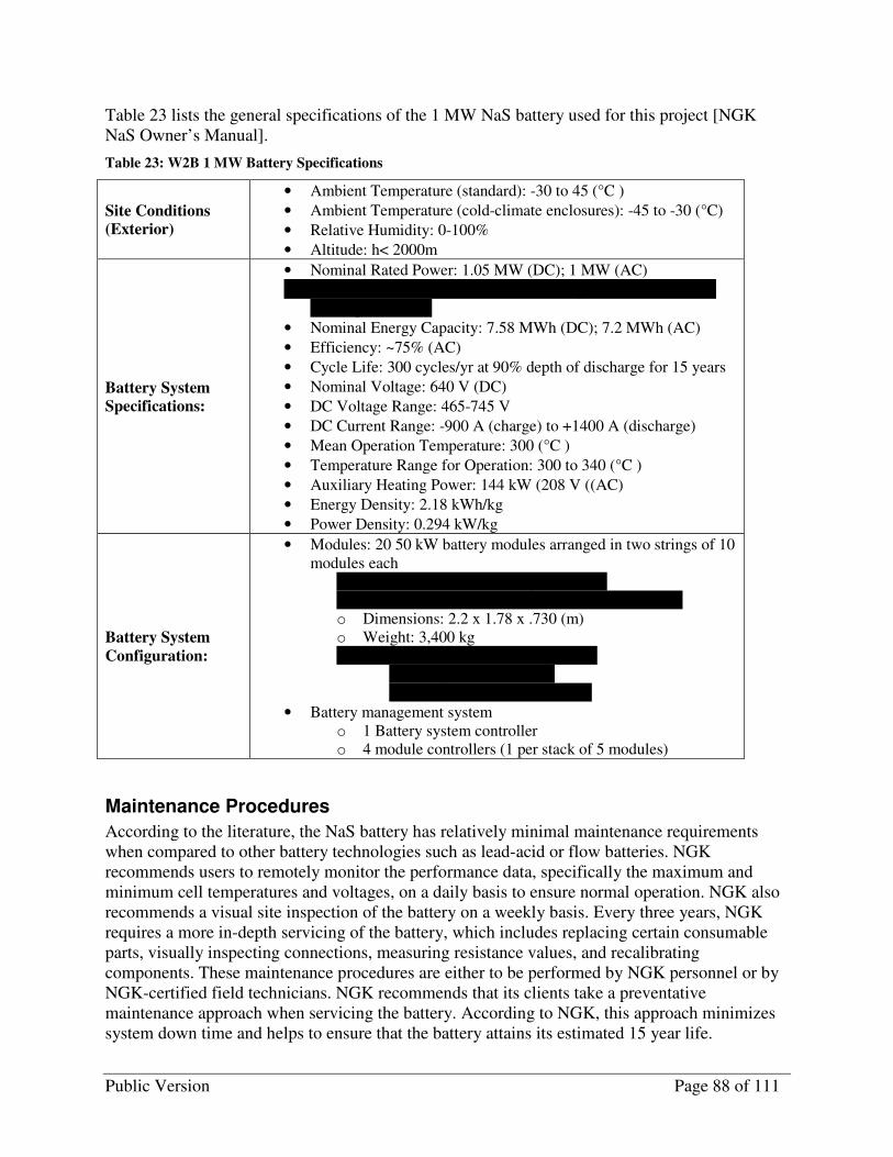
Public Version Page 88 of 111
Table 23 lists the general specifications of the 1 MW NaS battery used for this project [NGK NaS Owner’s Manual].
Table 23: W2B 1 MW Battery Specifications
Site Conditions
(Exterior)
• Ambient Temperature (standard): -30 to 45 (°C )
• Ambient Temperature (cold-climate enclosures): -45 to -30 (°C)
• Relative Humidity: 0-100%
• Altitude: h< 2000m
Battery System
Specifications:
• Nominal Rated Power: 1.05 MW (DC); 1 MW (AC)
• Maximum rated Power: 1.26 MW (DC) up to 3 hours; 1.1 MW (AC) up to 3 hours
• Nominal Energy Capacity: 7.58 MWh (DC); 7.2 MWh (AC)
• Efficiency: ~75% (AC)
• Cycle Life: 300 cycles/yr at 90% depth of discharge for 15 years
• Nominal Voltage: 640 V (DC)
• DC Voltage Range: 465-745 V
• DC Current Range: -900 A (charge) to +1400 A (discharge)
• Mean Operation Temperature: 300 (°C )
• Temperature Range for Operation: 300 to 340 (°C )
• Auxiliary Heating Power: 144 kW (208 V ((AC)
• Energy Density: 2.18 kWh/kg
• Power Density: 0.294 kW/kg
Battery System
Configuration:
• Modules: 20 50 kW battery modules arranged in two strings of 10 modules each
o Cell Connections: 8s x 11p x 4 blocks o Heat Loss: 2.2 to 3.4 kW depending on insulation o Dimensions: 2.2 x 1.78 x .730 (m) o Weight: 3,400 kg o # Freeze/Thaw Cycles (charge-end):
� 10 cycles (T<150 °C) � 30 cycles (150<T<250 °C)
• Battery management system o 1 Battery system controller o 4 module controllers (1 per stack of 5 modules)
Maintenance Procedures
According to the literature, the NaS battery has relatively minimal maintenance requirements when compared to other battery technologies such as lead-acid or flow batteries. NGK recommends users to remotely monitor the performance data, specifically the maximum and minimum cell temperatures and voltages, on a daily basis to ensure normal operation. NGK also recommends a visual site inspection of the battery on a weekly basis. Every three years, NGK requires a more in-depth servicing of the battery, which includes replacing certain consumable parts, visually inspecting connections, measuring resistance values, and recalibrating components. These maintenance procedures are either to be performed by NGK personnel or by NGK-certified field technicians. NGK recommends that its clients take a preventative maintenance approach when servicing the battery. According to NGK, this approach minimizes system down time and helps to ensure that the battery attains its estimated 15 year life.

Public Version Page 89 of 111
Power conversion system
Introduction
The PCS is a microprocessor-based system of power electronics, consisting of an inverter / rectifier (DC-to-AC and AC-to-DC converter) connected to a series of choppers40 (DC-to-DC converters). The PCS is connected in parallel with the NaS battery to automatically convert electricity back and forth between AC and DC for charging and discharging operations with the grid. The PCS also provides users with control functionality and system status information. The unit is designed for outdoor, unattended operation, and has local and remote control, monitoring, and data-archiving capabilities.
The PCS communicates with NGK’s master battery controller to control all operation functions related to the battery. The PCS has the ultimate responsibility of protecting the battery from damage due to excessive charging and/or discharging for all modes of operation. The PCS has a nominal continuous power rating of 1,250 kVA and connects to the local electric circuit via a three-phase 34.5 kV, wye-connected four-wire interconnection. The PCS is equipped with two Allen Bradley PM300 power meters: one monitors the charging and discharging operations of the battery, and the other monitors the auxiliary power draw of the battery module heaters and power electronics.
Nominal specifications for the DESS are summarized in Table 24 below:
Table 24: Nominal Specifications for DESS
Description Value
Nominal Real Power Capacity ±1,000 kW
Maximum Apparent Power Capacity ±1,250 kVA
Nominal Interconnection Voltage 34.5 kV (three-phase)
Current Rating 1504 A
Nominal DC Voltage Per String 640 V
DC Voltage Range Per String
Discharge 465 V
Charge 745 V
DC Current Range Per String41
Discharge 0 – 1400 A
Charge -900 – 0 A
Response Speed < 16 ms
Nominal Accuracy ±1% of kW/kVAR set-point
40 A chopper is a device that converts DC electricity from one voltage to another to either boost or buck system voltage.
41 The NGK battery controller treats positive as discharging and negative as charging, unlike the convention used elsewhere where positive is charging and negative is discharging.

Public Version Page 90 of 111
Physical Layout
The DESS is contained in three groups of enclosures: one group for the PCS equipment, a second enclosure for the 480:34.5kV transformer, and a third group for the NaS battery control equipment. The PCS equipment is contained in a group of four interconnected and adjoining enclosures.
Figure 57 is a picture of the enclosures, showing them both with their doors open and shut. The four enclosures (left to right) are: the DC interface bay, the inverter bay, the AC interface bay, and the control bay.
Figure 57: PCS Enclosures
Physical Operating Principles and Electrical Layout
At its core, the operating principle of the PCS is based on converter technology and controls developed around insulated gate bipolar transistors (IGBTs). To charge the battery, AC electricity from the grid passes through the PCS, where it is transformed into DC electricity and then stored in the battery. To discharge the battery, the PCS converts DC electricity from the battery into AC electricity and then supplies it to the grid.
Figure 58 is an electrical 1-line diagram of the PCS. For system protection, a DC circuit breaker is located between each NaS battery string and the PCS. Controlled by the PCS, the breakers allow the PCS to be isolated from the NaS battery for maintenance needs and to disconnect and shut down the battery as a protective measure if necessary. An 800 V(DC) bus is located between the choppers and the inverters and regulates power and voltage. The AC side of the inverter is connected to the 480V(AC) bus. A 1.25 MVA transformer boosts the voltage from 480 V to 34.5 kV to allow for the DESS to connect to the MWD bus42.
42 Please refer to the architecture section for an entire overview of the electrical connectivity of the battery and wind farm.
Figure is protected by Confidentiality Agreement with S&C

Public Version Page 91 of 111
1600 A
200
208 4W
480 4W
150 KVA
CT’s
1600:5
(3)Emergency Shutdown
Master Controller
Inverter
Chopper 1BChopper 1A Chopper 2A Chopper 2B
NAS Battery String 1 NAS Battery String 2
2000 A 2000 A
208V 3 Phase Heater power
465-745 VDC
1358 A max
465-745 VDC
1358 A max
1600A AC Breaker
Status, Green for
open, red for closed
34.5kV
480 4W
Figure 58: PCS and Battery One Line Diagram

Public Version Page 92 of 111
The PCS also contains a 208 V(AC) three-phase, wye-connected 150 kVA auxiliary transformer to provide power to the battery module heaters. Under normal operation, the AC grid powers this auxiliary transformer. However, in the event of a grid outage, a transfer switch adjacent to the battery will switch the power supply of the transformer from the grid to the backup generator so that the module heaters can continue to operate and maintain the battery modules at a safe operating temperature.
In addition to being compliant with the required codes and standards43, the PCS has several safety features embedded in its design. The PCS comes equipped with an emergency shutdown switch that performs a rapid but controlled shutdown of the DESS by opening up the DC and AC circuit breakers, which prevents the DESS from operating. In addition, the PCS monitors the battery ground connection and will disconnect itself from the NaS battery and issue an alarm to system operators in the event of a fault. Furthermore, the PCS also monitors temperature sensors located in each enclosure to ensure normal operating temperatures.
The PCS is designed to limit the current total harmonic distortion at the point of interconnection to less than 5% when the PCS is operating at a capacity of at least 500 kW for both charging and discharging modes of operation. The PCS is also protected from over-current and over-voltage transients and surges. Lastly, at no time will the PCS energize a grid during a system outage (i.e. it is not capable of islanding).
Unlike traditional grid-tied inverters that play a passive role in regulating system voltage, the DESS is a dynamic unit that is capable of providing and absorbing reactive power to and from the grid to regulate system voltage using real-time controls. A user-specified binary software bit allows the PCS to regulate system voltage either by responding to a voltage set-point (for the low-side of the 480V-34.5kV transformer) or a VAR set-point. With this capability, the DESS is able to assume a more autonomous role in supporting system voltage, while providing system operators with greater flexibility.
PCS Alarms
In the event of an extreme operating condition, the PCS will enter into an alarm state. The PCS categorizes alarms into two-levels of severity: low-severity (transient alarms) and high-severity (persistent alarms). The PCS recovers from low-severity alarms through an auto-restart function, which does not require corrective action from a person. High-severity or persistent alarms prohibit auto-restart, and require intervention and corrective action from an S&C engineer or certified technician. Irrespective of the fault type, the PCS HMI can be accessed for details about the type of alarm that has occurred, the likely root cause, the adjustments or repairs that might be needed, and whether or not the system may be reset and re-started.
The reset and restart function may be configured to respond to alarms in one of several ways. When configured for manual reset only, the PCS requires operator intervention through the HMI. When configured for auto-reset, the PCS reset command is automatically issued and re-issued a pre-determined number of times. If the PCS is not able to clear the fault within the pre-determined number of resets, the system will prohibit auto-restart and issue an alarm. Lastly, the PCS can be configured in a self-reset mode. In this mode, PCS operation automatically resumes when the issued alarm clears.
43 IEEE 1547, IEEE519-1993, IEEE C62.45-2002, IEEE C62.41.2-2002, IEEE C37.90.1-2002

Public Version Page 93 of 111
PCS HMI
The PCS comes equipped with an HMI that allows for a user to operate and troubleshoot the DESS. The HMI is a Linux-based embedded PC with a custom operating program designed by S&C. It enables an on-site operator to perform several functions on the DESS and is still accessible when the emergency shutdown switch is engaged.
A user can operate the DESS through the HMI by specifying the appropriate operating commands. In addition, the HMI provides the operator with detailed information on the real-time operating parameters of the system (e.g. voltage, current, and power), as well as trending information and any alarms. Furthermore, the HMI allows the operator to startup and shutdown the DESS to manage planned outages. Because the PCS is browser-based, it is accessible from any network-connected computer. As a result, the HMI can be accessed remotely by a user in possession of the appropriate access credentials.
All the PCS HMI screens and settings that are user-adjustable can be adjusted either locally or remotely. To establish a local connection, an operator is physically on-site and logged into the HMI. To establish a remote connection, an operator logs into the HMI via the Secure Shell (SSH) network protocol. This remote connection allows a remote operator to request system status information as well as to issue operating commands to the DESS.
PCS Modes of Operation
The DESS has three modes of operation: local-only, local-remote, and remote-only. The PCS categorization of the W2B modes of operation is listed in Table 25.
Table 25: PCS Types of Modes of Operation
For the Local-Only modes, the PCS responds to inputs from the local HMI only, ignoring all remote operating commands. In the Local Var Only Run mode, the DESS is capable of providing only reactive power and can respond to either a VAR set-point or voltage set-point. In the Local Power VAR Run mode, the DESS is capable of providing reactive power along with real power from a user specifying a specific kW command.
In the Local-Remote modes of operation, a user specifies the input settings for a particular mode of operation and the PCS determines the actual kW command. In the Remote-Only mode of operation, the PCS receives a kW command from a remote system operator and attempts to follow the signal to the best of its abilities. For reactive power in both the Local-Remote and Remote-Only modes of operation, a remote system operator specifies a voltage or VAR set-point for the DESS.
Local-Only Local-Remote Remote-Only
Local Var Only Run Basic GS Dispatch to Serve Frequency
Regulation
Local Power Var Run Wind Smoothing ED
Dispatched Wind Leveling
Emergency Charge
Test SOC
Public Version Page 94 of 111
PCS Server-Client Designation
The PCS has two masters that can write set-points to it. The first master is the local RCY remote terminal unit (RTU) that relays production data from the wind farm to the PCS. The second master is GridPoint, which serves the role of the remote external controller. To prevent one master from inadvertently over-riding a set-point written by the other, the RCY RTU and the GridPoint master can write only to set-points that have been assigned to them. In addition, both masters have a “watch-dog” timer for the PCS that consists of a rolling counter that updates every second. If the timer of either master is not updated after 20 seconds, the PCS equates this as loss of communication with that respective master and will enter into the appropriate default mode of operation. The PCS interface with both masters is carried out using DNP3. These interfaces are discussed in greater detail in the system architecture section.
Maintenance and System Lifetime
S&C has designed the PCS to perform over an extended period of time with minimal maintenance requirements. S&C estimates the PCS system lifetime at 20 years.
S&C provides remote monitoring services that consist of an S&C engineer monitoring the PCS on a daily basis to identify and report any potential system malfunctions involving the PCS. If a malfunction does occur, the S&C engineer will troubleshoot the PCS.
Maintenance of the PCS includes a series of monthly and yearly checks on the device to ensure proper operation. Every 30-60 days, a technician needs to replace the air filter in the PCS. On a yearly basis, an Xcel Energy field technician needs to visually inspect the PCS components for any significant or unusual wear and tear, verify connections at all the terminals, verify appropriate control set-points and system settings, and check for rust.
DESS Overall System Efficiency
The overall efficiency of the DESS depends on multiple factors such as the mode of operation, the efficiency of the battery modules, the efficiency of the PCS, and ambient weather conditions. To get a baseline of the efficiency of the unit, project analysts measured the DC efficiency (i.e. the electrochemistry efficiency) and the AC efficiency (with and without the auxiliary load) for a 24-hour period using a standard daily charge-discharge profile while varying the depth of discharge. For this specific test, project participants did not account for any impacts of ambient weather conditions.
The team designated 1,ACη to measure the overall efficiency of the DESS, which accounts for the
amount of AC energy the PCS discharged ( ACdMWh , ), the amount of AC energy the PCS used
to charge ( ACcMWh , ), and the energy draw of the auxiliary loads ( ACauxMWh , ). The team
designated 2,ACη to measure only the efficiency of the DESS when the auxiliary energy draw
was excluded. Analysts designated DCη to calculate the efficiency of the battery modules (i.e. the
electrochemistry efficiency) by measuring the amount of DC energy into and out of the battery
modules ( DCdMWh , and DCcMWh , ).
ACauxACc
ACd
ACMWhMWh
MWh
,,
,
1,+
=η

Public Version Page 95 of 111
ACc
ACd
ACMWh
MWh
,
,
2, =η
DCc
DCd
DCMWh
MWh
,
,=η
Figure 59 displays the efficiency values for varying depths of discharge over a 24 hour period.
As shown by the figure, the 1,ACη efficiency is heavily dependent on the amount of time that the
DESS operates within the time period of interest due to two primary reasons made evident by Table 26.
Figure 59: Overall System
Efficiency
Table 26: DESS Efficiency Test Data
First, when the DESS is idle, the NaS module temperatures fall at an accelerated rate compared to when the DESS operates, as discussed previously. As a result, the module heaters are required to operate at a greater frequency to keep the module temperatures within the required range.
Second, with less charge-discharge operation, ACauxMWh , becomes a larger contribution to the
efficiency calculation relative to ACdMWh , and ACcMWh , . The 2,ACη efficiency does not appear to
Performance Data Efficiency
Depth of Discharge
AC Charge (MWh)
AC Discharge
(MWh)
AC Auxiliary
(MWh)
DC Charge (MWh)
DC Discharge
(MWh) η1 η2 ηDC
90% 8.57 7.03 0.24 8.25 7.22 79.9% 82.1% 87.5%
70% 6.60 5.54 0.42 6.34 5.69 78.9% 83.9% 89.8%
50% 4.75 4.01 0.77 4.56 4.11 72.6% 84.4% 90.1%
30% 2.87 2.45 0.94 2.76 2.48 64.3% 85.3% 89.7%
10% 1.00 0.84 1.09 0.96 0.83 40.2% 83.9% 85.9%
0%
10%
20%
30%
40%
50%
60%
70%
80%
90%
100%
0% 20% 40% 60% 80% 100%
Depth of Discharge
Eff
icie
ncy
eta_1 eta_2 eta_dc
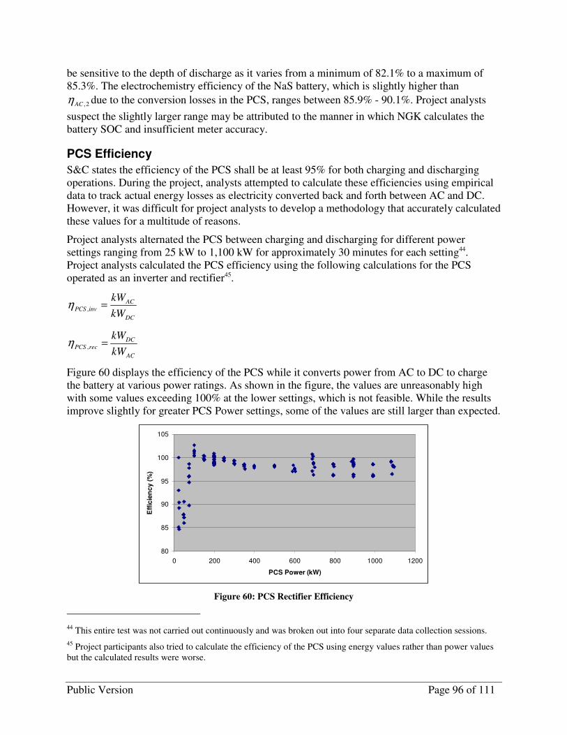
Public Version Page 96 of 111
be sensitive to the depth of discharge as it varies from a minimum of 82.1% to a maximum of 85.3%. The electrochemistry efficiency of the NaS battery, which is slightly higher than
2,ACη due to the conversion losses in the PCS, ranges between 85.9% - 90.1%. Project analysts
suspect the slightly larger range may be attributed to the manner in which NGK calculates the battery SOC and insufficient meter accuracy.
PCS Efficiency
S&C states the efficiency of the PCS shall be at least 95% for both charging and discharging operations. During the project, analysts attempted to calculate these efficiencies using empirical data to track actual energy losses as electricity converted back and forth between AC and DC. However, it was difficult for project analysts to develop a methodology that accurately calculated these values for a multitude of reasons.
Project analysts alternated the PCS between charging and discharging for different power settings ranging from 25 kW to 1,100 kW for approximately 30 minutes for each setting44. Project analysts calculated the PCS efficiency using the following calculations for the PCS operated as an inverter and rectifier45.
DC
AC
invPCSkW
kW=,η
AC
DC
recPCSkW
kW=,η
Figure 60 displays the efficiency of the PCS while it converts power from AC to DC to charge the battery at various power ratings. As shown in the figure, the values are unreasonably high with some values exceeding 100% at the lower settings, which is not feasible. While the results improve slightly for greater PCS Power settings, some of the values are still larger than expected.
80
85
90
95
100
105
0 200 400 600 800 1000 1200
PCS Power (kW)
Eff
icie
nc
y (
%)
Figure 60: PCS Rectifier Efficiency
44 This entire test was not carried out continuously and was broken out into four separate data collection sessions.
45 Project participants also tried to calculate the efficiency of the PCS using energy values rather than power values but the calculated results were worse.

Public Version Page 97 of 111
Figure 61 displays the efficiency of the PCS while it converts power from DC to AC to discharge the battery at various power ratings. Again, the values are unreasonably high with some values exceeding 100% at the lower settings. While the results improve slightly for greater PCS Power settings, some of the values are still larger than expected. A phenomenon that is also apparent in both graphs is that the variance of calculated efficiencies for small and large power levels is larger than those calculated for power settings between 200 kW and 600 kW.
80.0
85.0
90.0
95.0
100.0
105.0
-1200-1000-800-600-400-2000
PCS Power (kW)
Eff
icie
ncy (
%)
Figure 61: PCS Inverter Efficiency
Xcel Energy discussed these results with the National Renewable Energy Lab (NREL), S&C, and NGK, but unfortunately there was not a definitive explanation either for the invalid results or the variable ranges in efficiencies for the various power levels. NGK has experienced higher than expected PCS efficiency values in Japan as well and suspects it may have something to do with an error in which AC power is measured by the meter due to the presence of harmonic currents. S&C also mentioned that the accuracy and granularity of the meters installed in the PCS may not be sufficient enough for accurate efficiency measurements, especially at lower operating levels.

Public Version Page 98 of 111
DESS System Architecture
Introduction
In addition to evaluating the DESS technology, another primary focus of the W2B Project was to design and implement a communication system that enabled an external system aggregator to manage the operation of multiple distributed energy resources (DER) located within the same balancing area. Even though the project had only one DESS, Xcel Energy wanted a communication system that supported the virtual power plant concept, in which multiple DER units are aggregated into one effective resource that a grid operator can call upon to provide grid services. Because a virtual power plant would connect to a utility via a single interface, the company would not have to alter its communication system every time a new DER unit came online. In addition, grid operators could issue commitment and dispatch decisions for the entire DER pool rather than having to individually manage each unit.
Functional Requirements
The principal functional requirement for the W2B communication system was to enable remote control, monitoring, and data acquisition of the DESS. This requirement was driven by two project needs. First, due to the siting location of the battery, company employees based out of Minneapolis or Denver could not physically access the site with ease. Second, Xcel Energy wanted to design the system in a manner that aligned with other smart grid initiatives within the company.
Overview
The W2B Project was the first time Xcel Energy interfaced with an external system aggregator via the NSP EMS. The W2B Communication team, which consisted of individuals from Xcel Energy, S&C, and GridPoint, designed and implemented the communication system from July 2008 to May 2009.
Figure 62 on the next page is an architectural diagram of the system. The team had to create several interfaces for the project that involved multiple communication protocols, transport mechanisms, and source and destination applications. Furthermore, the design implemented the required security and encryption features to prevent any malicious network attacks on the system from outside users46.
The W2B communication design utilizes multiple communication circuits. Due to inadequate coverage from DSL, the communication team purchased a full T1 line at the site for internet connectivity. A 56k frame relay circuit over a dedicated leased line runs from Minneapolis, MN to Alexandria, VA to connect EMS MN and GridPoint for the external system aggregator functionality. Finally, another 56k frame relay circuit over a dedicated leased line runs from Sioux Falls, SD to Luverne, MN to provide Xcel Energy’s Angus Anson generation facility a SCADA connection to the DESS site for monitoring and system responder purposes.
46 Xcel Energy’s Enterprise Security department approved the design of the W2B communication system.
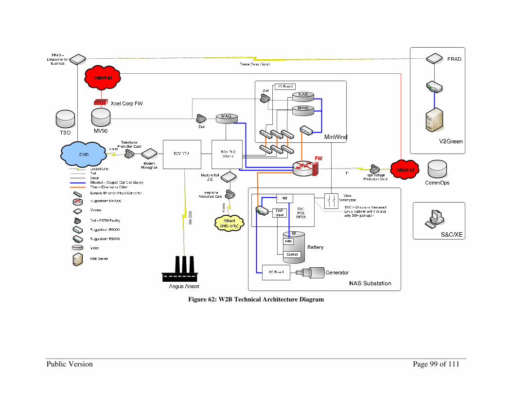
Public Version Page 99 of 111
4 wire
56k DDS
Figure 62: W2B Technical Architecture Diagram
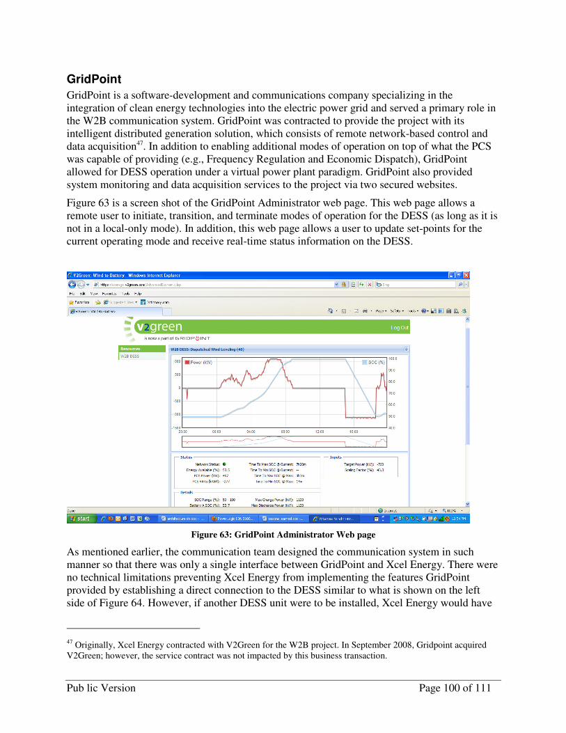
Pub lic Version Page 100 of 111
GridPoint
GridPoint is a software-development and communications company specializing in the integration of clean energy technologies into the electric power grid and served a primary role in the W2B communication system. GridPoint was contracted to provide the project with its intelligent distributed generation solution, which consists of remote network-based control and data acquisition47. In addition to enabling additional modes of operation on top of what the PCS was capable of providing (e.g., Frequency Regulation and Economic Dispatch), GridPoint allowed for DESS operation under a virtual power plant paradigm. GridPoint also provided system monitoring and data acquisition services to the project via two secured websites.
Figure 63 is a screen shot of the GridPoint Administrator web page. This web page allows a remote user to initiate, transition, and terminate modes of operation for the DESS (as long as it is not in a local-only mode). In addition, this web page allows a user to update set-points for the current operating mode and receive real-time status information on the DESS.
Figure 63: GridPoint Administrator Web page
As mentioned earlier, the communication team designed the communication system in such manner so that there was only a single interface between GridPoint and Xcel Energy. There were no technical limitations preventing Xcel Energy from implementing the features GridPoint provided by establishing a direct connection to the DESS similar to what is shown on the left side of Figure 64. However, if another DESS unit were to be installed, Xcel Energy would have
47 Originally, Xcel Energy contracted with V2Green for the W2B project. In September 2008, Gridpoint acquired V2Green; however, the service contract was not impacted by this business transaction.

Pub lic Version Page 101 of 111
to replicate the entire interface and individually manage and operate each battery. The external system controller functionality provided by GridPoint allows Xcel Energy to avoid implementing changes to its systems as additional DER units come online. As shown on the right side of Figure 64, the external system controller will setup a communication link to the new unit and then report to Xcel Energy the total MW and MWh capacity currently available from the pool of resources it has connectivity to. Depending on the control mode, the external system aggregator can either relay a dispatch command from Xcel Energy to the pool, or it can issue its own command in an automated fashion by embedding logic on a server.
Figure 64: External System Aggregator Concept
As with all designs, the W2B communication system does have some limitations. For this project, GridPoint’s intelligent distributed generation solution did not include responsibility for responding to system alarms. GridPoint only reported alarms to the appropriate stakeholders. As a result, the SCADA connection between Angus Anson and the DESS site was required.
Moreover, the DNP3 communication protocol is a sequentially polling protocol. Therefore, it is not possible for GridPoint to provide time-synchronized data from multiple data sources, which can complicate analytical tasks. Another drawback in the communication system is that there is no onsite data caching. Thus, when GridPoint loses communication with any of the devices or the T1 circuit goes down, there is no way to collect and archive data, resulting in incomplete datasets. Each week, project analysts tracked the availability and latency of GridPoint’s communication with the PCS in the executive summary reports.
System Context
Figure 65 on the next page is the system context diagram for the entire communication system. This diagram displays the source and destination of all the data flows. For purposes of simplification, a description of the data flows broken down by mode of operation is included on subsequent pages.
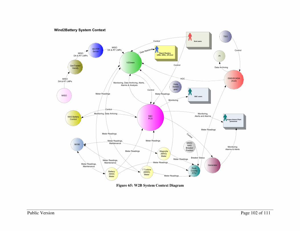
Public Version Page 102 of 111
V2Green
S&C
PCSNAS Battery
Control
Battery
(NAS)
Meter
EMS/SCADA
(Xcel)
7 Turbine
(MWD)
Meter
AGC
Magnolia
(MAG)
Meter
Monitoring, Data Arhiving
Meter Readings,
MaintenanceMeter Readings,
Maintenance
Meter Readings,
Maintenance
Control
Monitoring, Data Archiving, Alerts,
Alarms & Analysis
Meter Readings
Meter Readings
Meter Readings
GenTrader/
Versify
MISO
DA & RT LMPs
Rock
County
RTU
Meter Readings
Monitoring
PI
MV90
Meter Readings
MISO
MISO
DA & RT LMPs
Meter Readings
Control
Wind2Battery System Context
Report Readers
U/Min, NREL, GPI,Xcel
Xcel usersControl
S&C users
Generator
Meter Readings
Control
Meter Readings
MWD/
NAS
Breaker
Position
TSO
Angus Anson Plant
personnel
Monitoring,
Alerts and Alarms
XE FTP
Server
MISO
DA & RT LMPs
Data Archiving
Meter Readings
Breaker Status
Monitoring
Alarms & Alerts
Control
Vista
Switch
gear
Control
Data Ret
rieval
Figure 65: W2B System Context Diagram

Public Version Page 103 of 111
Basic GS
Figure 66 provides a layout of the data flow for the Basic GS (both wind-only and wind and grid charging) mode of operation. A system dispatcher logs in to GridPoint’s administrator web page, selects the desired Basic GS mode of operation, and specifies the “Basic GS Parameters”. The Basic GS parameters consist of the peak demand hour(s), wind scaling factor, discharge profile, and allowed charging times (including, if applicable, when charging from the grid is permissible)48. GridPoint relays the Basic GS parameters to the PCS, which uses the parameters to determine the appropriate magnitude and timing for charging and discharging operation. Xcel Energy’s TSO department sends either a kVAR or voltage set-point (depending on the configuration of the PCS) to GridPoint via EMS MN. GridPoint relays this set-point along to the PCS. Revenue grade metering information for both the battery and wind farm are sent to EMS MN by way of the RCY RTU. The RCY RTU also sends the power output of the wind facility to the PCS. GridPoint, TSO, EMS MN, and the system dispatcher all receive status information on the DESS in real-time.
Figure 66: System Context Flow for Basic GS Mode of Operation
48 The maximum and minimum allowed SOC values can be specified for each mode of operation; as a result they are not explicitly mentioned when listing the available user-configurable parameters for each mode.

Public Version Page 104 of 111
Wind Smoothing
Figure 67 provides a layout of the data flow for the Wind Smoothing mode of operation. A system dispatcher logs in to GridPoint’s administrator web page, selects this mode, and specifies the “Wind Smoothing Parameters”. The Wind Smoothing parameters consist of the wind scaling factor and the time constant for the 1st order lag function used by the PCS. GridPoint relays the Wind Smoothing parameters to the PCS, which uses the parameters to determine the appropriate magnitude and timing for charging and discharging operation. All other functionality is identical to that discussed in the description of the Basic GS mode of operation.
Figure 67: System Context Flow for Wind Smoothing Mode of Operation
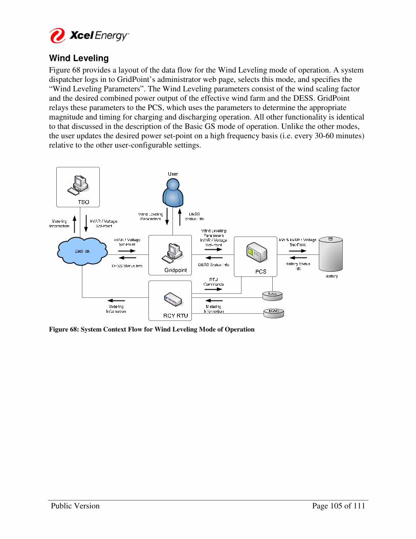
Public Version Page 105 of 111
Wind Leveling
Figure 68 provides a layout of the data flow for the Wind Leveling mode of operation. A system dispatcher logs in to GridPoint’s administrator web page, selects this mode, and specifies the “Wind Leveling Parameters”. The Wind Leveling parameters consist of the wind scaling factor and the desired combined power output of the effective wind farm and the DESS. GridPoint relays these parameters to the PCS, which uses the parameters to determine the appropriate magnitude and timing for charging and discharging operation. All other functionality is identical to that discussed in the description of the Basic GS mode of operation. Unlike the other modes, the user updates the desired power set-point on a high frequency basis (i.e. every 30-60 minutes) relative to the other user-configurable settings.
Figure 68: System Context Flow for Wind Leveling Mode of Operation

Public Version Page 106 of 111
Frequency Regulation
Figure 69 provides a layout of the data flow for the Frequency Regulation mode of operation. A system dispatcher logs in to GridPoint’s test administrator web page, selects this mode, and specifies the “AGC Parameters”. The AGC parameters consist of the ACE scaling factor (“Scaling Factor”), the upper ACE dead-band factor (“AceDb_BatU”), and the lower ACE dead-band factor (“AceDb_BatL”). GridPoint relays this information to EMS MN along with real-time status information on the PCS. In addition to data it receives from GridPoint, EMS MN also receives the real-time ACE values from MISO via its existing Inter-Control Center Communications Protocol (ICCP) connection. EMS MN uses this information to generate a four-second frequency regulation signal within its AGC system for the DESS to follow. EMS MN sends this command to GridPoint who relays it on to the PCS. All other functionality is identical to that discussed in the description of the Basic GS mode of operation.
Figure 69: System Context Flow for Frequency Regulation Mode of Operation

Public Version Page 107 of 111
Economic Dispatch
Figure 70 provides a layout of the data flow for the ED mode of operation. A system dispatcher logs in to GridPoint’s test administrator web page, selects this mode, and specifies the “Economic Dispatch Parameters”. The ED parameters are the most detailed of any of the required inputs from a system dispatcher, consisting of settings charge and discharge settings and rates for various SOC levels and pricing scenarios in the energy markets. In addition to the information GridPoint receives from the system dispatcher, it also receives daily award and pricing information from Xcel Energy’s Commercial Operations department via an Xcel Energy-hosted FTP server. GridPoint uses this information to determine the appropriate magnitude and timing of charge and discharge signals when the battery is in the ED mode of operation. All other functionality is identical to that discussed in the description of the Basic GS mode of operation.
Figure 70: System Context Flow for ED Mode of Operation

Public Version Page 108 of 111
References Denholm, Paul et al. “The Role of Energy Storage With Renewable Electricity Generation”. National Renewable Energy Laboratory. January 2010.
EPRI-DOE Handbook of Energy Storage for Transmission and Distribution Applications, EPRI, Palo Alto, CA, and the U.S. Department of Energy, Washington DC: 2003
Kirby, Brendan J. “Frequency Regulation Basics and Trends”. Oak Ridge National Laboratory. December 2004.
Lutz, Brad etal. Xcel Energy Wind2Battery Project: Data Analysis Report (Draft). National Renewable Energy Laboratory. January 2010.
Makarov, Y.V., et al. “Assessing the Value of Regulation Resources Based on Their Time Response Characteristics”. Pacific Northwest National Laboratory. June 2008.
North American Electric Reliability Corporation (NERC). “Accommodating High Levels of High Variable Generation. April 2009.
Ortech Power. “Wind Power Forecasting Pilot Project Part B: The Quantitative Analysis Final Report”. Submitted to The Alberta Electric System Operator. August 8, 2008.
Walawalkar, Dr. Rahul. “Market Analysis of Emerging Electric Energy Storage Systems”. National Energy Technology Laboratory. July 31, 2008.

Public Version Page 109 of 111
List of Acronyms
Acronym Definition ACE Area Control Error
AGC Automatic Generation Control
Ah Ampere-hours
ASM Ancillary Service Market
BMS Battery Management System
CAES Compressed Air Energy Storage
CO2 Carbon Dioxide
CPNode Commercial Price Node
DA Day-Ahead (a MISO energy market)
DER Distributed Energy Resource
DESS Distributed Energy Storage System
DNP3 Distributed Network Protocol 3.0
DOD Depth of Discharge
DSL Digital Subscriber Line
ED Economic Dispatch
EMS Energy Management System
FERC Federal Energy Regulatory Commission
FTP File Transfer Protocol
GPI Great Plains Institute
GS Generation Storage
HMI Human-Machine Interface
ICCP Inter-Control Center Communications Protocol
IGBT Insulated Gate Bipolar Transistors
LMP Locational Marginal Price
MISO Midwest ISO
MP Market Participant
MWD Minwind Energy LLC
NaS Sodium Sulfur
NERC North American Electric Reliability Corporation
NGK NGK Insulators, LTD
NREL National Renewable Energy Lab
NSP Northern States Power
OCV Open Circuit Voltage
PCS Power conversion system
PLC Programmable logic controller
RCY Rock County
RGOS Regional Generator Outlet Study
RSG Revenue Sufficiency Guarantee
RT Real-Time (a MISO energy market)
RTU Remote Terminal Unit
S&C S&C Electric
SER Stored Energy Resource
SOC State of Charge
TSO Transmission Systems Operations
V Volts
W2B Wind To Battery Project
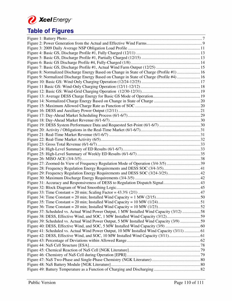
Public Version Page 110 of 111
Table of Figures Figure 1: Battery Photo................................................................................................................................. 7 Figure 2: Power Generation from the Actual and Effective Wind Farms..................................................... 9 Figure 3: 2009 Daily Average NSP Obligation Load Profile ..................................................................... 11 Figure 4: Basic GS, Discharge Profile #1, Fully Charged (12/11) ............................................................. 13 Figure 5: Basic GS, Discharge Profile #1, Partially Charged (12/15) ........................................................ 13 Figure 6: Basic GS Discharge Profile #4, Fully-Charged (1/8) .................................................................. 14 Figure 7: Basic GS, Discharge Profile #1, Actual Wind Farm Output (12/25) .......................................... 15 Figure 8: Normalized Discharge Energy Based on Change in State of Charge (Profile #1) ...................... 16 Figure 9: Normalized Discharge Energy Based on Change in State of Charge (Profile #4) ...................... 16 Figure 10: Basic GS: Wind Only Charging Operation (12/24-12/25) ........................................................ 17 Figure 11 Basic GS: Wind-Only Charging Operation (12/11-12/12) ......................................................... 18 Figure 12: Basic GS: Wind-Grid Charging Operation (12/30-12/31)........................................................ 19 Figure 13: Average DESS Charge Energy for Basic GS Mode of Operation............................................. 19 Figure 14: Normalized Charge Energy Based on Change in State of Charge ............................................ 20 Figure 15: Maximum Allowed Charge Rate as Function of SOC .............................................................. 20 Figure 16: DESS and Auxiliary Power Output (12/11) .............................................................................. 21 Figure 17: Day-Ahead Market Scheduling Process (6/1-6/7)..................................................................... 29 Figure 18: Day-Ahead Market Revenue (6/1-6/7) ...................................................................................... 30 Figure 19: DESS System Performance Data and Requested Set-Point (6/1-6/7) ....................................... 30 Figure 20: Activity / Obligations in the Real-Time Market (6/1-6/7)......................................................... 31 Figure 21: Real-Time Market Revenue (6/1-6/7) ....................................................................................... 31 Figure 22: Real-Time Market Activity (6/5)............................................................................................... 32 Figure 23: Gross Total Revenue (6/1-6/7) .................................................................................................. 33 Figure 24: High-Level Summary of ED Results (6/1-6/7).......................................................................... 33 Figure 25: High-Level Summary of Weekly ED Results (6/1-6/7) ............................................................ 35 Figure 26: MISO ACE (3/4-3/5)................................................................................................................. 38 Figure 27: Zoomed-In View of Frequency Regulation Mode of Operation (3/4-3/5) ................................ 39 Figure 28: Frequency Regulation Energy Requirements and DESS SOC (3/4-3/5)................................... 41 Figure 29: Frequency Regulation Energy Requirements and DESS SOC (3/24-3/25)............................... 42 Figure 30: Maximum Discharge Energy Requirements (3/4-3/5) .............................................................. 42 Figure 31: Accuracy and Responsiveness of DESS to Regulation Dispatch Signal................................... 43 Figure 32: Block Diagram of Wind Smoothing Logic................................................................................ 45 Figure 33: Time Constant = 20 min; Scaling Factor = 43.3% (2/1) ........................................................... 47 Figure 34: Time Constant = 20 min; Installed Wind Capacity = 1 MW (2/15).......................................... 50 Figure 35: Time Constant = 20 min; Installed Wind Capacity = 10 MW (1/24)........................................ 51 Figure 36: Time Constant = 20 min; Installed Wind Capacity = 10 MW (1/23)........................................ 52 Figure 37: Scheduled vs. Actual Wind Power Output, 1 MW Installed Wind Capacity (3/12) ................. 58 Figure 38: DESS, Effective Wind, and SOC, 1 MW Installed Wind Capacity (3/12)................................ 59 Figure 39: Scheduled vs. Actual Wind Power Output, 5 MW Installed Wind Capacity (3/9) ................... 59 Figure 40: DESS, Effective Wind, and SOC, 5 MW Installed Wind Capacity (3/9) ................................. 60 Figure 41: Scheduled vs. Actual Wind Power Output, 10 MW Installed Wind Capacity (3/11) ............... 61 Figure 42: DESS, Effective Wind, and SOC, 10 MW Installed Wind Capacity (3/11).............................. 61 Figure 43: Percentage of Deviations within Allowed Range...................................................................... 62 Figure 44: NaS Cell Structure [ESA].......................................................................................................... 78 Figure 45: Chemical Reaction of NaS Cell [NGK Literature].................................................................... 79 Figure 46: Chemistry of NaS Cell during Operation [EPRI] ...................................................................... 79 Figure 47: NaS Two-Phase and Single-Phase Chemistry (NGK Literature) .............................................. 80 Figure 48: NaS Battery Module [NGK Literature] ..................................................................................... 80 Figure 49: Battery Temperature as a Function of Charging and Discharging ............................................ 82

Public Version Page 111 of 111
Figure 50: Outage Response Time as Function of Depth of Discharge [NaS Instruction Manual]............ 82 Figure 51: Reference Discharge Profiles .................................................................................................... 84 Figure 52: Example of Standard NGK Battery Operation .......................................................................... 84 Figure 53: Example of Non-Standard NGK Battery Operation.................................................................. 85 Figure 54: NGK Cycle Counting Logic...................................................................................................... 85 Figure 55: NaS Cycle Life as a Function of Depth of Discharge [EPRI] ................................................... 86 Figure 56: NaS Battery Object Hierarchy................................................................................................... 87 Figure 57: PCS Enclosures ......................................................................................................................... 90 Figure 58: PCS and Battery One Line Diagram.......................................................................................... 91 Figure 59: Overall System Efficiency......................................................................................................... 95 Figure 60: PCS Rectifier Efficiency ........................................................................................................... 96 Figure 61: PCS Inverter Efficiency............................................................................................................. 97 Figure 62: W2B Technical Architecture Diagram...................................................................................... 99 Figure 63: GridPoint Administrator Web page......................................................................................... 100 Figure 64: External System Aggregator Concept ..................................................................................... 101 Figure 65: W2B System Context Diagram ............................................................................................... 102 Figure 66: System Context Flow for Basic GS Mode of Operation ......................................................... 103 Figure 67: System Context Flow for Wind Smoothing Mode of Operation............................................. 104 Figure 68: System Context Flow for Wind Leveling Mode of Operation ................................................ 105 Figure 69: System Context Flow for Frequency Regulation Mode of Operation..................................... 106 Figure 70: System Context Flow for ED Mode of Operation................................................................... 107
Table of Tables Table 1: Modes of Operation ........................................................................................................................ 8 Table 2: 2009 Monthly Peak Demand Hours.............................................................................................. 10 Table 3: Maximum Allowed Charge Rates................................................................................................. 12 Table 4: Basic GS System Performance Data Statistics Summary............................................................. 22 Table 5: Basic GS Selected Discharge Results ........................................................................................... 23 Table 6: Basic GS: Wind Only Selected Charging Performance Data ....................................................... 23 Table 7: Basic GS: Wind and Utility Selected Charging Performance Data .............................................. 23 Table 8: Basic GS All Discharge Results ................................................................................................... 24 Table 9: Basic GS: Wind Only All Charging Performance Data................................................................ 25 Table 10: Basic GS: Wind and Utility All Charging Performance Data .................................................... 26 Table 11: Economic Dispatch System Performance Data Statistics Summary .......................................... 34 Table 12: MISO ACE Statistics .................................................................................................................. 39 Table 13: DESS Frequency Regulation Performance Statistics (3/4-3/5) .................................................. 40 Table 14: Frequency Regulation System Performance Data Statistics Summary....................................... 44 Table 15: Effective Wind and Total Ramping Statistics for Selected Ramping Periods............................ 49 Table 16: DESS Ramping Statistics for Selected Ramping Periods........................................................... 49 Table 17: Wind Smoothing System Performance Data Statistics Summary .............................................. 53 Table 18: Effective Wind and Total Ramping Statistics for all Ramping Periods ..................................... 54 Table 19: DESS Ramping Statistics for all Ramping Periods .................................................................... 55 Table 20: Relative Allowed Deviations in Scheduled vs. Actual Wind Power as a Function of Wind Capacity ...................................................................................................................................................... 62 Table 21: Wind Leveling System Performance Data Statistics Summary.................................................. 63 Table 22: NaS Battery Pros and Cons......................................................................................................... 77 Table 23: W2B 1 MW Battery Specifications ............................................................................................ 88 Table 24: Nominal Specifications for DESS .............................................................................................. 89 Table 25: PCS Types of Modes of Operation ............................................................................................. 93 Table 26: DESS Efficiency Test Data......................................................................................................... 95