SludgePro Cloud Manual

1.1 Introduction SludgePro is a cloud-based software that reads, filters and plots the height

of the sludge measured in waste stabilisation ponds/lagoons with survey

tools.

The application is cloud-based with a logical user interface for easy

manipulation of files for each pond, and has a backend script based in

MATLAB to perform all of the calculations and plot.

The user interface guides the user into providing the information

necessary to process, analyse and visualise survey data. Also, all files and

data can be read and modified by the user without any programming

knowledge.

1.2 Login to SludgePro To access SludgePro, go to:

sludgeanalytics.com

Navigate to and click on the SludgePro software icon.

Note: The software will not open in Internet Explorer. Use a browser such

as Google Chrome or Mozilla Firefox.

The following login screen will appear (Figure 1.1). Log in using the

username and password provided.

Figure 0.1

SludgePro login window

1.3 Adding a Pond/Lagoon Navigate to the Manage Ponds tab as seen in Figure 1.2.

On the left pane, complete the form, following the instructions below:

Enter a Pond Name: Add a name for the pond.

KML File for Pond Perimeter: Select a KML file for the perimeter of the

pond. These can be drawn in Google Earth Pro©. Please see Section

1.4.6 (“Creating a KML file”) for information on how to create a

KML file.

Enter Depth (m): Enter the depth from asset data. If unsure of the

depth, enter a guess.

Enter rotation (degrees): Non-North facing ponds can be rotated in

SludgePro to allow better visualisation of the data. Ponds need to be

manually rotated as the default is to plot ponds according to their GPS

location, see Figure 1.3. Rotation is the angle between -90 and 90 (in

degrees) the pond faces with respect to North (default is 0 degrees)

(Figure 1.4). Can be checked using “View x/y”

Rotate About (South or West point): Allows you to choose which corner

of the pond to pivot the rotation around. Can be checked using “View

x/y”

Figure 0.2 Manage ponds tab.

angle

N

Figure 0.3

Example of a north facing pond system.

Figure 0.4

Example of a pond system that is non-north facing. In yellow, the angle to input into the rotation section. In this case a rotation to the left = -30 degrees.

1.4 Processing survey data

1.4.1 Adding a sampling period

To process survey data, you will first need to add a sampling period. This

can be done by navigating to the Manage Sampling Period tab across

the top navigation pane (Figure 1.5).

To add a new sampling period:

1. Select the pond you wish to add a sampling period for from the

Pond Name drop down menu.

2. Enter the Start date and End date of the profiling period. For

example if the profiling is completed on 1 January 2019, then the

start and end date are the same. Dates may be typed in as

DD/MM/YYYY format, or can be selected using the drop down

calendar.

3. Add any Comments about the survey. This could include relevant

weather conditions, areas that could not be accessed, operation

issues, etc.

4. Click on Add Period.

5. The sampling period will now appear on the right. This sampling

period may be edited or deleted as required using the buttons

located under Action on the right hand side..

Figure 0.5

Adding a sampling period

1.4.2 Adding survey data

The next step to process data is to upload the survey data to the server.

This can be done by navigating to the Manage Data Files tab across the

top navigation pane (Figure 1.6).

To upload data:

1. Select the pond you wish to upload data for from the Pond Name

drop down menu.

2. Select the Sampling Period from the drop down menu.

3. Water level above/below standard operating level (m): If it is known

that the pond water level is higher or lower than normal, please

indicate this here using + values for above and – values for below.

If the water level is normal, please enter 0.

4. Navigate to and choose the csv data file you wish to be uploaded

under Data Files. Only one file may be selected each time.

5. Click on Add File.

6. If more than one file, repeat steps 1-5.

7. Once a file is added the pane on the right will populate (Figure 1.7).

Figure 0.6

Uploading data files

More than one file may be added for the same pond, so long as the files

are <50MB in size.

If you want to check the survey coverage of the file uploaded (if you have

several files for the same pond) then click on View under the Action

column on the right side.

If you have uploaded a file in error, you may delete is using the Delete

option.

Figure 0.7

Manage data files tab with uploaded data files shown on the right.

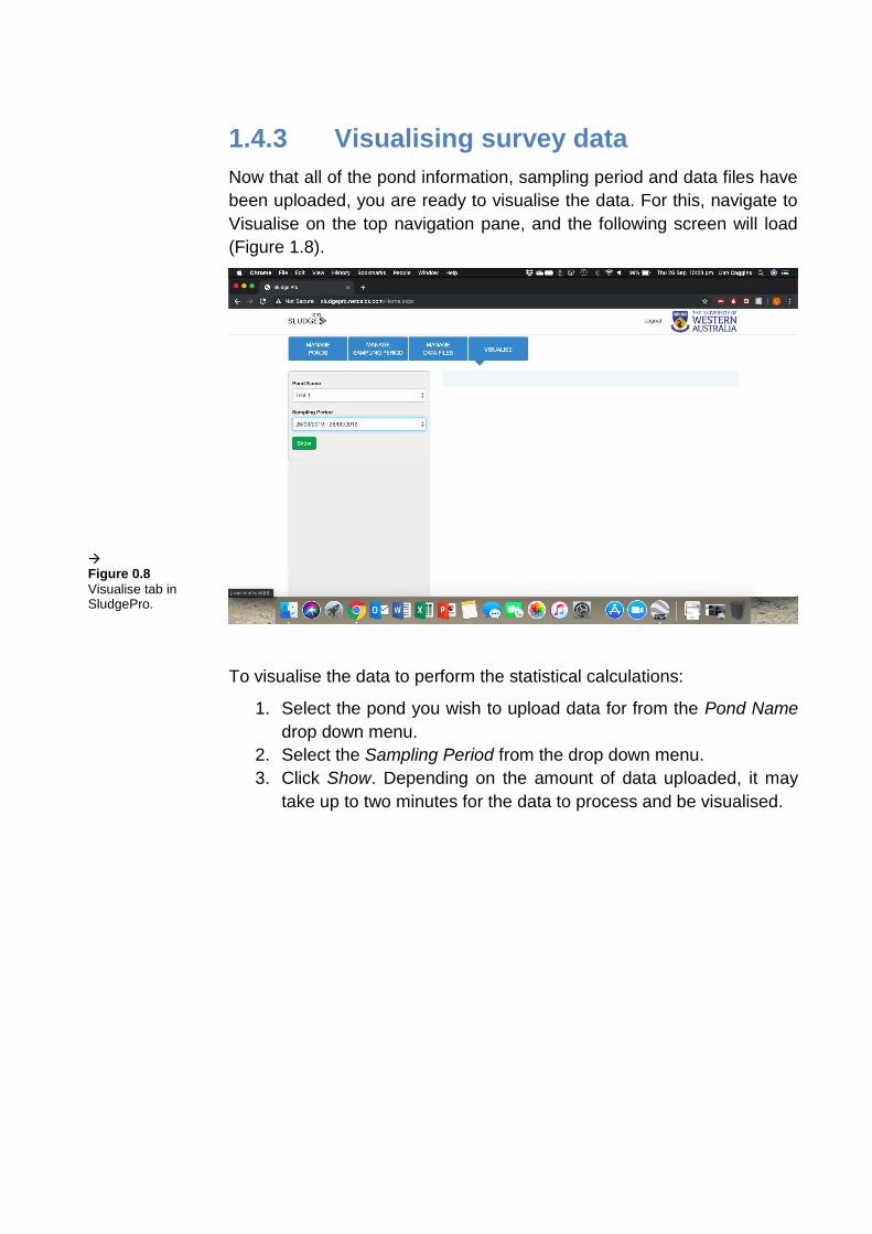
1.4.3 Visualising survey data

Now that all of the pond information, sampling period and data files have

been uploaded, you are ready to visualise the data. For this, navigate to

Visualise on the top navigation pane, and the following screen will load

(Figure 1.8).

To visualise the data to perform the statistical calculations:

1. Select the pond you wish to upload data for from the Pond Name

drop down menu.

2. Select the Sampling Period from the drop down menu.

3. Click Show. Depending on the amount of data uploaded, it may

take up to two minutes for the data to process and be visualised.

Figure 0.8

Visualise tab in SludgePro.

Once processing has completed, a screen like the following will appear

(Figure 1.9).

The default first screen shown on the right is that of a 3D surface of the water depth measured.

On the left navigation pane, you will find the following options:

Data points: This shows the data points plotted. If the depth of the pond entered at the beginning is too shallow, you may find sections of the pond do not have any blue x plotted there. In order to fix this, navigate back to Manage Ponds and edit the pond depth for the pond in question. Then navigate back to Visualise and let the calculations run again.

Water depth contours (as surveyed)

Sludge thickness contours (Depth – water depth)

3D Water Depth

3D Sludge Thickness

X Cross-section: SludgePro will plot 4 equidistant cross-sections along the x, which are indicated by the lines overlayed over the contour shown. These lines then correspond to the graph shown below.

Y Cross-section: Same as with the X, but in the Y direction.

Analytics: Under this tab you will find the following information o Pond depth (m): As entered when you added the pond

originally, this is the depth that is assumed for sludge volume calculations

o Total area (m2): Surface area of the pond, as traced using Google Earth (from the KML file added).

o Pond volume (m3): Pond depth × Total area o Water volume (m3): From survey data, the volume of water

calculated in the pond. o Sludge volume (m3): Pond volume - water volume

Figure 0.9

Visualise tab after data has been processed.

o Sludge infill (%): Sludge volume / Pond volume o Min water depth (m): Minimum water depth (to sludge) o Max water depth (m): Maximum water depth o Ave water depth (m): Average water depth o Area filled about 66%: Statistic to have a better under standing

of distribution of sludge in the pond o Area filled above 50%: As above o Area filled below 25% As above

PDF Report: You can generate a PDF report for the data visualised by selecting PDF report, and then selecting whether you would like to view data based upon water depth or sludge thickness. You can also enter you name, so that others know who the report was generated by.The PDF report will display the Sludge thickness and Water depth contours, as well as the X and Y cross sections based upon water depth/sludge thickness (depending on what you selected). It will also display a table of all of the statistics calculated. An example is shown below (Figure 1.10).

1.4.4 Analytics

If you have more than one sampling period recorded for a pond, you will

be able to see the trend in sludge infill, etc. in the Analytics tab. The titles

for:

o Water volume (m3) o Sludge volume (m3) o Sludge infill (%): o Min water depth (m) o Max water depth (m)

Figure 0.10

Example of PDF output generated in SludgePro.

o Ave water depth (m) o Area filled about 66% o Area filled above 50% o Area filled below 25%

Will appear in red, and you will be able to click on them. Clicking on each

of these headings will make a graph load below the table, showing you the

trend for that particular parameter over time.

1.4.5 Modify a pond

To modify the parameter of a pond navigate back to the Manage Ponds

menu, find the pond on the list, and click on Edit Pond.

1.4.6 Creating a KML file

To create a KML file you need to use Google Earth. Find the pond and

click on the icon Add Path. A pop up window will appear and the path

should be named with the pond name (e.g., Pond1). Then, DO NOT close

that window and start tracing the path around the pond until you close the

polygon by double clicking near the end. Click Ok. It will then save this

path to the temporary places on the sidebar in Google Earth. Right click

on this file and press Save Place As. A window will pop up. Name the file

with the pond name (e.g. Pond1) select type as kml. NOTE: kmz is the

default format, so you will need to change it to kml.

1.5 Troubleshooting The cloud-based SludgePro is new, and we are still looking for issues! If

you have any issue please contact: liah.coggins@uwa.edu.au

If the issue has caused a red box to appear in the top right hand corner of

the screen, please screenshot and send this to us, and we will try to sort

out the problem as soon as possible.