slide 1 t:/classes/bms602b/lecture 3 602_b.ppt © 1995-2004 j.paul robinson - purdue university...

t:/classes/BMS602B/lecture 3 602_B.ppt© 1995-2004 J.Paul Robinson - Purdue UniversityPurdue University Cytometry Laboratories

Week 4BME 695Y / BMS 634

Confocal Microscopy: Techniques and Application Module

Image Structure and 2D image Analysis Principles

& Sample Preparation Techniques

Purdue University Department of Basic Medical Sciences, School of Veterinary Medicine

& Department of Biomedical Engineering, Schools of Engineering

J.Paul Robinson, Ph.D.Professor of Immunopharmacology & Biomedical Engineering

Director, Purdue University Cytometry Laboratories

These slides are intended for use in a lecture series. Copies of the graphics are distributed and students encouraged to take their notes on these graphics. The intent is to have the student NOT try to reproduce the figures, but to LISTEN and UNDERSTAND

the material. All material copyright J.Paul Robinson unless otherwise stated, however, the material may be freely used for lectures, tutorials and workshops. It may not be used for any commercial purpose.

One useful text for this course is Pawley “Introduction to Confocal Microscopy”, Plenum Press, 2nd Ed. A number of the ideas and figures in these lecture notes are taken from this text.


Digital image analysis is Data Analysis.

• Data files are a representation of an original image, which is itself a representation of reality.

• The chain of digital image processing includes both creation of digital data from an image, and recreation of an image from the digital data.

• Data file formats are created in order to make specific operations more convenient. The most convenient format may differ with the particular application.

• For most purposes, a one-to-one mapping of pixels to data values is most useful, but the internal representation of the data values may be different for different file formats.

• Files can be either compressed, or not, and compression can be either lossy or not. For scientific analysis lossy compression is unacceptable; it may be useful for overview presentations.

• Image manipulation can take place before image acquisition, during image acquisition, on the digital data, or during recreation of an output image.• Simple image manipulation includes brightness or contrast variation, re-sizing, median filtering, and spatial kernel filtering.

• Brightness and contrast variation are controlled by a system input-output curve. Spatial kernel filtering and median filtering use information local to a particular area of an image to modify that area.


How an image is created


Noise removal


How do humans classify objects?

Human method is pattern recognition based upon multiple exposure to known samples. We build up mental templates of objects, this image information coupled with other information about an object allows rapid object classification with some degree of objectivity, but there is always a subjective element.

We are sensitive to differences in contrast. We will tend to overestimate the amount or size of an object if there is high contrast vs low contrast. We are sensitive to perspective and depth changes We are sensitive to orientation of lighting. We prefer light to come from above. We fill in what we think should be in the image


This illustration was first published in 1861 by Ewald Hering. Astronomers became very interested in Hering's work because they were worried that visual observations might prove unreliable.


This illusion was created in 1889 by Franz Müller-Lyon. The lengths of the two identical vertical lines are distorted by reversing the arrowheads. Some researchers think the effect may be related to the way the human eye and brain use perspective to determine depth and distance, even though the objects appear flat.


In 1860 Johann Poggendorff created this line distortion illusion. The two segments of the diagonal line appear to be slightly offset in this figure.


An ambiguous image by the Dutch artist Gustave Verbeek


The above figure represents a series of 3 pixel x 3 pixel kernels. Many image processing procedures will perform operations on the central (black) pixel by using use information from neighboring pixels. In kernel A, information from all the neighbors is applied to the central pixel. In kernel B, only the strong neighbors, those pixels vertically or horizontally adjacent, are used. In kernel C, only the weak neighbors, or those diagonally adjacent are used in the processing. It is various permutations of these kernel operations that form the basis for digital image processing.


modifying image contrast and brightness

• The easiest and most frequent method is histogram manipulation

• An 8 bit gray scale image will display 256 different brightness levels ranging from 0 (black) to 255 (white). An image that has pixel values throughout the entire range has a large dynamic range, and may or may not display the appropriate contrast for the features of interest.


It is not uncommon for the histogram to display most of the pixel values clustered to one side of the histogram or distributed around a narrow range in the middle. This is where the power of digital imaging to modify contrast exceeds the capabilities of traditional photographic optical methods. Images that are overly dark or bright may be modified by histogram sliding. In this procedure, a constant brightness is added or subtracted from all of the pixels in the image or just to a pixels falling within a certain gray scale level ( i.e. 64 to 128).


A somewhat similar operation is histogram stretching in which all or a range of pixel values in the image are multiplied or divided by a constant value. The result of this operation is to have the pixels occupy a greater portion of the dynamic range between 0 and 255 and thereby increase or decrease image contrast. It is important to emphasize that these operations do not improve the resolution in the image, but may have the appearance of enhanced resolution due to improved image contrast.


Histogram Stretching


A B

Histogram sliding and stretching


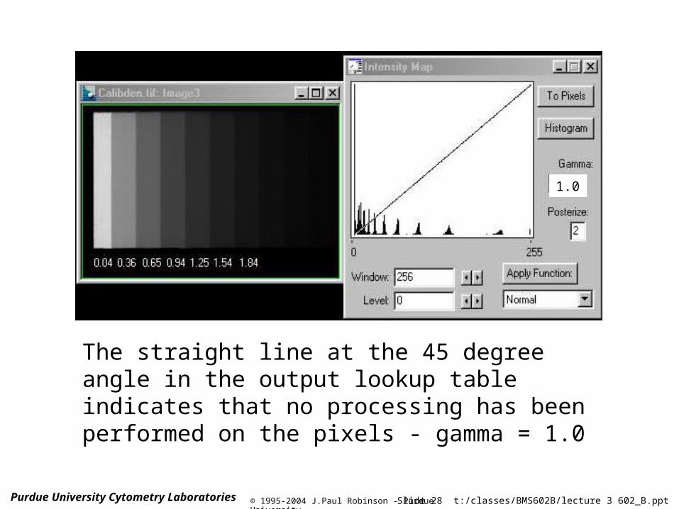
Gamma - The gamma of a histogram curve is the slope, expressed as a ratio of the logs of the output to input values. A gamma value of 1.0 equals an output:input ratio of 1:1 and no correction is applied. In some programs, a gamma function applies a lookup table function to compensate or correct for the bias which may be built into the video source. A camera's light response is often set to a power function (Gamma function) to mimic the photometric response of the human eye. This may result in a non-linear response from the video source and cause errors if you are making densitometric measurements. The camera bias can be removed by applying an inverse gamma function. This function calculates a lookup table to correct for the bias based on operator provided parameters. The gamma function for decalibrating the camera can be obtained from the camera manufacturer.


1.0

The straight line at the 45 degree angle in the output lookup table indicates that no processing has been performed on the pixels - gamma = 1.0


In this image a gamma factor of 1.8 has been applied to the histogram of the output LUT histogram


In this image a gamma factor of 2.2 has been applied to the histogram of the output LUT histogram


Inverse function applied to previous image


Arbitrary adjustment to the output LUT histogram


Removing noise in an Image

Images collected under low illumination conditions may have a poor signal to noise ratio. The noise in an image may be reduced using image averaging techniques during the image acquisition phase. By using a frame grabber and capturing and averaging multiple frames (e.g. 16 to 32 frames) the information in the image may be increased and the noise decreased. Cooled CCD cameras have a better signal to noise ratio that non-cooled CCD cameras. Noise in a digital image may also be decreased by utilizing spatial filters.


Filters such as averaging and gaussian filters will reduce noise, but also cause some blurring of the image. The use of these filters on high resolution images is usually not acceptable. Median filters cause minimal blurring of the image and may be acceptable for some electron microscopic images. These filters use a kernel such as a 3 x 3 or 5 x 5 to replace the central or target pixel luminance value with the median value of the neighboring pixels. The effect is a blending of the brightness of the pixels within a selection. The filter discards pixels that are too different from adjacent pixels.


Remove dirt and noise with a 3 x 3 median filter


Periodic noise in an image may be removed by editing a 2-dimensional Fourier transform (FFT). A forward FFT of the image below, will allow you to view the periodic noise (center panel) in an image. This noise, as indicated by the white box, may be edited from the image and then an inverse Fourier transform performed to restore the image without the noise (right panel).


Remove periodic noise with fast

fourier transforms


Pseudocolor image based upon

gray scale or luminance

Human vision more sensitive to color. Pseudocoloring makes it is possible to see slight variations in gray scales


Image Analysis: After adjustment for contrast and brightness, and noise, the next phase of the process is feature identification and classification.

Most image data may be classified into areas that feature closed boundaries (e.g. a cell), points - discrete solid points or objects that may be areas, and linear data. For objects to be identified they must be segmented and isolated from the background. It is often useful to convert a gray scale image to binary format (all pixel values set to 0 or 1). Techniques such as image segmentation and edge detection are easily carried out on binary images but may also be performed on grayscale or color images.


Simplest method for image segmentation is to use thresholding techniques.

Thresholding may be performed on monochrome or color images. For monochrome images, pixels within a particular grayscale range or value may be displayed on a computer monitor and the analysis performed on the displayed pixels.

Greater discrimination may be achieved using color images. Image segmentation may be achieved based upon red, green, and blue (RGB) values in the image, or a more powerful method is to use hue, saturation and intensity (HSI).


inte

nsity

hue

0°

saturation

black

whiteThe HSI method of color discrimination is closer to how the human brain discriminates colors. Hue = is the wavelength of light reflected from or transmitted through an object. Saturation = purity of the color and represents the amount of gray in proportion to the hue - 0% (gray) to 100% (fully saturated). Intensity = Relative lightness or darkness - 0 (black) , 100 (white)


Image thresholding based on RGB or HIS

Hue – Saturation - Intensity


Threshold objects of interest


Preparation Techniques, stereo and 3D Imaging

UPDATED February 2002


Characteristics of Fixatives• Chemical Fixatives• Freeze Substitution• Microwave Fixation

Ideal FixativePenetrate cells or tissue rapidly

Preserve cellular structure before cell can react to produce structural artifacts

Not cause autofluorescence, and act as an antifade reagent


Chemical Fixation• Coagulating Fixatives

• Crosslinking Fixatives

Coagulating Fixatives• Ethanol

• Methanol

• Acetone


Coagulating Fixatives

• Fix specimens by rapidly changing hydration state of cellular components

• Proteins are either coagulated or extracted

• Preserve antigen recognition often

Advantages

Disadvantages• Cause significant shrinkage of specimens

• Difficult to do accurate 3D confocal images

• Can shrink cells to 50% size (height)

• Commercial preparations of formaldehyde contain methanol as a stabilizing agent


Crosslinking Fixatives

• Glutaraldehyde

• Formaldehyde

• Ethelene glycol-bis-succinimidyl succinate (EGS)

• Form covalent crosslinks that are determined by the active groups of each compound


Glutaraldehyde• First used in 1962 by Sabatini et al*• Shown to preserve properties of subcellular structures by EM• Renders tissue autofluorescent so less useful for fluorescence

microscopy, but fluorescence can be attenuated by NaBH4.

• Forms a Schiff’s base with amino groups on proteins and polymerizes via Schiff’s base catalyzed reactions

• Forms extensive crosslinks - reacts with the -amino group of lysine, -amino group of amino acids - reacts with tyrosine, tryptophan, histidine, phenylalanine and cysteine

• Fixes proteins rapidly, but has slow penetration rate• Can cause cells to form membrane blebs

*Sabatini, D.D., et al, “New means of fixation for electron microscopy and histochemistry. j. hISTOCHEM.cYTOCHEM. 37:61-65.


Glutaraldehyde

• Supplied commercially as either 25% or 8% solution

• Must be careful of the impurities - can change fixation properties - best product from Polysciences (Worthington, PA)

• As solution ages, it polymerizes and turns yellow.

• Store at -20 °C and thaw for daily use. Discard.


Formaldehyde• Crosslinks proteins by forming methelene bridges between reactive groups• The ratelimiting step is the de-protonation of amino groups, thus the pH dependence of

the crosslinking• Functional groups that are reactive are amido, guanidino, thiol, phenol, imidazole and

indolyl groups• Can crosslink nucleic acids• Therefore the preferred fixative for in situ hybridization• Does not crosslink lipids but can produce extensive vesiculation of the plasma

membrane which can be averted by addition of CaCl2

• Not good preservative for microtubules at physiologic pH• Protein crosslinking is slower than for glutaraldehyde, but formaldehyde penetrates 10

times faster.• It is possible to mix the two and there may be some advantage for preservation of the

3D nature of some structures.


Ethelene glycol-bis-succinimidyl succinate (EGS)

• Crosslinking agent that reacts with primary amino groups and with the epsilon amino groups of lysine

• Advantage is its reversibility

• Crosslinks are cleavable at pH 8.5

• Mainly used for membrane bound proteins

• Limited solubility in water is a problem


Fixation and preparation of tissue

• Solutions– 8% glutaraldehyde EM grade

– 80 mM Kpipes, pH 6.8, 5 mM EGTA, 2 mM MgCl2, both with and without 0.1% Triton X-100 (triton for cytoskeletal proteins)

– PBS Ca++/Mg++ free

– PBS Ca++/Mg++ free, pH 8.0

• When using glutaraldehyde 8% - open new vial, dilute to 0.3% in solution of 80 mM Kpipes, pH 6.8, 5 mM EGTA, 2 mM MgCl2, 0.1% triton X-100. Store aliquots at -20°C. Never re-use once thawed out.


Fixation ProtocolpH-shift/Formaldehyde

• Method developed for fixing rat brain

• Excellent preservation of neuronal cells and intracellular compartments

• Formaldehyde is applied twice - once at near physiological pH to halt metabolism and second time at high pH for effective crosslinking


Method• Solutions

– 40% formaldehyde in H2O (Merck)

– 80 mM Kpipes, pH 6.8, 5 mM EGTA, 2 mM MgCl2

– 100 mM NaB4 O7 pH 11.0

– PBS Ca++/Mg++ free

– PBS Ca++/Mg++ free, pH 8.0 (plus both with and without 0.1% Triton X-100

– premeasured 10 mg aliquots of dry NaBH4

– see detailed methods page 314 of Pawley , 2nd ed.


Fluorescence Labeling• There are no “standard” methods for all

cells - each cell type will be different.

• It is useful to use vital labeled specimens to determine changes induced by the fixation procedure– e.g.: Rhodamine 123 [mitochondria]

– 3,3’-dihexyloxaccarbo-cyanine (DiOC6) [ER]

– C6-NBD-ceramide [Golgi]


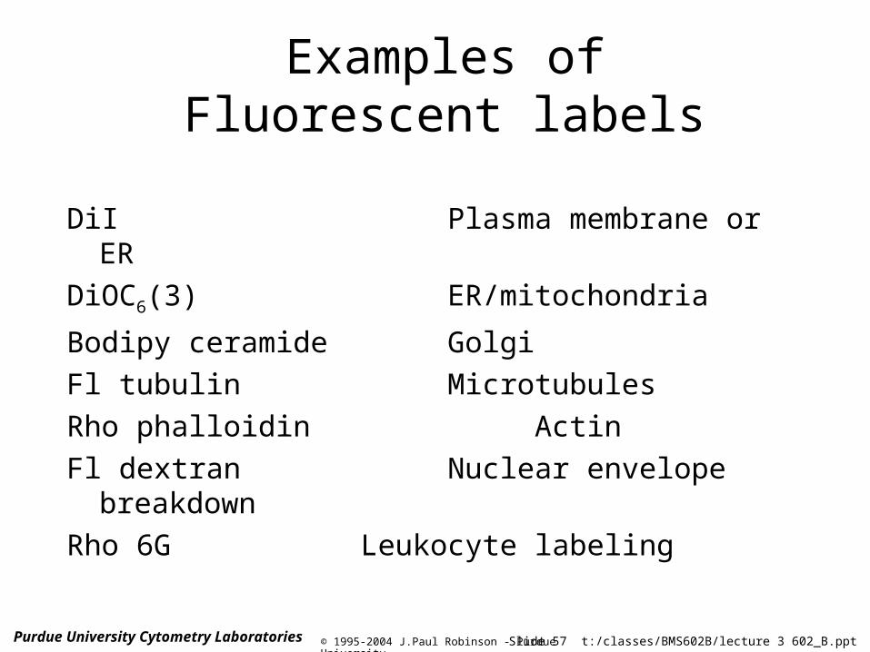
Examples of Fluorescent labels

DiI Plasma membrane or ER

DiOC6(3) ER/mitochondria

Bodipy ceramide Golgi

Fl tubulin Microtubules

Rho phalloidin Actin

Fl dextran Nuclear envelope breakdown

Rho 6G Leukocyte labeling


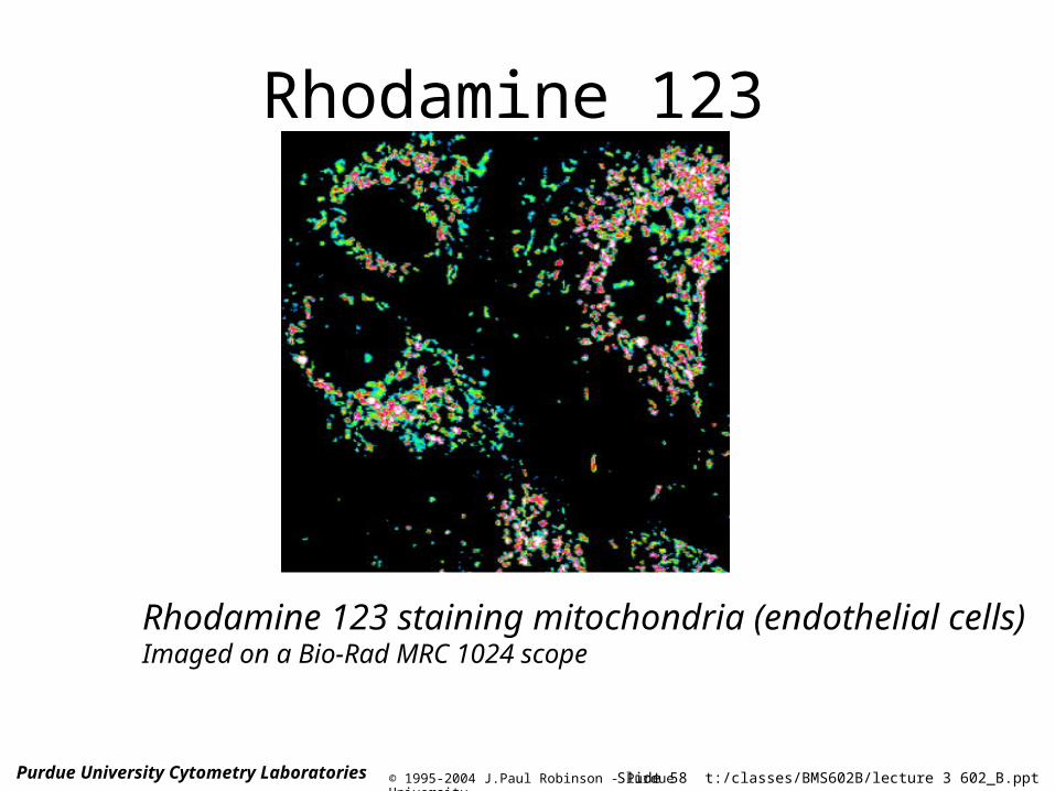
Rhodamine 123

Rhodamine 123 staining mitochondria (endothelial cells)Imaged on a Bio-Rad MRC 1024 scope


Test Specimen

• According to Terasaki & Dailey (p330,

Pawley, 2nd ed) a convenient test specimen for a living cell is onion epithelium

• Stain with DiOC6(3) (stock solution is 0.5 mg/ml in ethanol. For final stain dilute 1:1000 in water

• Stains ER and mitochondria


Test Specimen - Onion

Peel off epithelium

Stain with DiOC6(3)

ER and Mitochondria stainedModified from Pawley, “Handbook of Confocal Microscopy”, Plenum Press


Test images

Onion Fluorescence ImagesImaged on a Bio-Rad MRC 1024 scope


3D Imaging and 3D Reconstruction techniques

z

x

y

# z sections =#images


z

x

y

z

yy

3D Image Reconstruction


x

y

z

y

y

z

3D Image Reconstruction


Pine Tree pollen - collected on a Bio-Rad MRC 1024 at Purdue University Cytometry Laboratories

© J.Paul Robinson - Purdue University Cytometry Laboratories


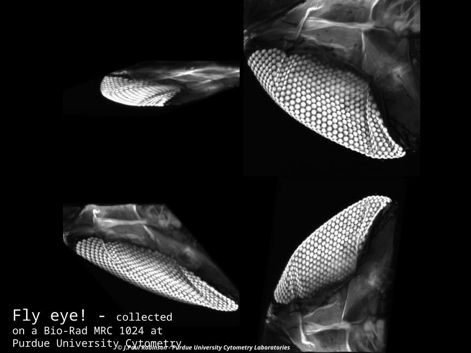
Fly eye! - collected on a Bio-Rad MRC 1024 at Purdue University

Cytometry Laboratories © J.Paul Robinson - Purdue University Cytometry Laboratories


Collagen fibers collected using transmitted light and fluorescence [collected on a Bio-Rad MRC 1024 at Purdue University Cytometry Laboratories ]


3D visualization tools


Stereo Imaging

There are two methods for creating stereo pairs:

1. Use different colors for each image eg. Anaglyphs of red-green which produce a monochrome 3D image

2. Side-by-side display of both images


Creating Stereo pairs

z

xy

Pixel shifting -ive pixel shift for left+ive pixel shift for right


• Top: Endothelial cells (live) cultured on a coverslide chamber. The cells were stained with stain that identified superoxide production (hydroethidine) and were color coded (red =high stain, green =low stain) then a 3D reconstruction performed and a vertical slice of the culture shown. Here, the original image was collected with many more pixels - so the magnified image looks better!

• Left: Same endothelial cells with hydroethidine stain (live cells) showing a fluorescence reconstruction - note fluorescence is only in nuclear regions - no cytoplasm is stained. Imaged on Bio-Rad MRC 1024 system.

• Top: Endothelial cells (live) cultured on a coverslide chamber. The cells were stained with stain that identified superoxide production (hydroethidine) and were color coded (red =high stain, green =low stain) then a 3D reconstruction performed and a vertical slice of the culture shown. Here, the original image was collected with many more pixels - so the magnified image looks better!

• Left: Same endothelial cells with hydroethidine stain (live cells) showing a fluorescence reconstruction - note fluorescence is only in nuclear regions - no cytoplasm is stained. Imaged on Bio-Rad MRC 1024 system.


Calculation and Measurement in 3D Imaging

• Depth and Thickness

• Length, Area and Volume

• Surface Area

• Fluorescence Intensity


Depth and Thickness

• Axial resolution is related to the square of the NA so use highest NA lens possible

• Refractive Index (RI) must (should!) be same between sample, and lens


Real and apparent depth

Diagram modified from Confocal Microscopy: Methods and Protocols Ed. Stephen Paddock, Humana Press 1999 p362 Fig 3)

Apparent depth2 mmReal depth

3 mm

Focus shift 2 mm


Summary• Structure of images & Image formats• Image Processing techniques• Image Analysis Techniques• Good confocal images require good preparation techniques• Preparations is the most significant factor in image quality• Preparation techniques can damage the 3D structure of specimens• Quality control of specimen preparation requires attention to

protocols• To create 3D structure requires careful imaging• Stereo images are rapid techniques for visualization• Quantitative imaging requires accurate collection information

slide 1 t:/classes/bms602b/lecture 3 602_b.ppt © 1995-2004 j.paul robinson - purdue university...

Documents

image acquisition

output image

original image

data analysis

simple image manipulation

data values

data files

creation of digital