SLAC-PUB-5593 December 1991

T/E

A Plumber’s View of Perturbative &CD*

J. D. BJORKEN

Stanford Linear Accelerator Center

Stanford University, Stanford, California 94309

ABSTRACT

The fractal phase space introduced by the Lund group for the description of

QCD multijet phenomena is discussed using a different choice of coordinates. We

advocate these coordinates as a useful diagnostic tool in the analysis of complex

event structures. Features of QCD such as color-coherence or “angular ordering,”

and the “string effect,” are described in this language.

Submitted to Physical Review D.

* Work supported by the Department of Energy, contract DE-AC03-76SF00515.

1. Introduction

The so-called lego plot, introduced to the best of my knowledge by some anony-

mous hero within the UAl collaboration, has taken its place as an important di-

agnostic tool in contemporary particle physics. This occurs because for many pur-

poses the most convenient variables to describe particle, parton, or jet coordinates

are the rapidity y (or pseudo-rapidity q), azimuthal angle q5 relative to the collision

axis (or, in e +e- applications, the thrust axis), and magnitude of the momentum

transverse to that axis, pt. The reasons for this choice include the following:

1. Invariant phase-space is simply described with this choice:

d3P - = ptdptdy d$ . E

2. These variables have simple transformation properties under longitudinal

Lorentz boosts

Pt + Pt c-4 y + y + const . P-2)

3. The populations of produced particles are, in the absence of QCD jets, dis-

tributed very uniformly in the variables y and 4, while they are rather sharply

centered in pt about the mean value (pt).

It is especially this third feature that motivated much work [l] in the early 1970s on

building an analogy between populations of produced particles in the y - q5 plane

with populations of particles in a 2-dimensional fluid. On average, uniform density

is expected in each case and, to large extent, this has been found experimentally.

2

With the advent of QCD, this picture has changed somewhat. The emission of

perturbative gluons by the partons participating in the underlying collision process

leads to clustering in the lego plot, and on occasion to strong concentrations of pt

(jets) within small regions of y and 4.

In an interesting series of papers [2] , G us a sson t f and his Lund collaborators

have shown how this leads to an extension of the ordinary phase space to one which

is fractal in nature and which provides, even in the presence of QCD jet phenomena,

a way of maintaining a uniform measure (produced particle density) in the extended

phase space. It is the purpose of this paper to elaborate on this approach, using

coordinates somewhat different than employed by the Lund group, but which we

find more convenient. The main point is simply the suggestion that fractal phase

space, using this choice of variables, may be a convenient and practical diagnostic

tool in the phenomenological analysis of multiparticle and multijet processes at

high energy.

In Section 2, we review the properties of the lego variables 17 and 4. In Section

3, we introduce jets into the lego plot, along with a definition of jets which leads to

the extension into fractal phase space. Section 4 is devoted to kinematics, where

the same multijet production phenomenology is viewed from a variety of reference

frames. Section 5 is devoted to a more geometrical view of extended phase space,

using an analogy to plumbing. In Section 6 we extend the picture to include

the leading-logarithm multijet description of perturbative QCD. In Section 7, we

describe in plumber’s language the “color-coherence,” or “angular-ordering” effects

present in QCD. Section 8 is devoted to an illustration of these ideas using the well-

known “string effect” in the processes eSe- t qqg and e+e- + qi.jy. In Section 9,

we make a few comments regarding hadron-hadron collisions. Concluding remarks

3

are contained in Section 10.

2. A Review of Lego Variables

In a high-energy fixed-target experiment almost all particles are produced at

small angles. If we place a screen transverse to the incident beam direction and

downstream of the target, the particle distribution impinging on that screen will

be nonuniform. However, if we subdivide it as shown in Fig. l(a), then within

each cell the mean number of particles will be roughly the same. Note that in Fig.

l(a) we have divided the azimuth into nine sectors, so that

A$ = 2n/9 = 0.698 M 0.70 . (24

Likewise the radial coordinate, essentially 8, is subdivided by factors 2, so that the

pseudorapidity 7’

77 = - log tan 8/2 (24

is divided, to excellent accuracy, into subintervals of the same size:

Aq = log 2 = 0.693 = 0.7 .

Actually the mean number of particles per cell as defined here is

(n) = 0.5 gj = g (f) < 1 77

P-3)

(24

even at SSC energies.

1 We shall not explicitly distinguish the rapidity y from pseudorapidity q in what follows.

4

lb)

701

A B C

A B C rl- 6%4Al

Figure 1. (a) Phase-space as seen in fixed-target geometry. (b) The same phase space as described in the lego variables 17 and q5.

The virtue of the usual lego plot is that it maps this picture into rectangular

77 - q5 coordinates, as shown in Fig. l(b), because the resultant particle density

is approximately uniform when expressed in this way, and the element of area is

proportional to the phase-space area.

5

3. Jets

A jet is a local concentration of produced particles in v,d space with a total

transverse-momentum pt in excess of some minimum value, typically at least a few

GeV.

There are a variety of possible algorithms for defining jets, but for our purposes

it is convenient [3] to define a jet as all particles within a circle in the Zego plot with

radius 0.7, provided the summed pt within the circle exceeds the threshold value.

To be sure, this algorithm does not state how to precisely choose the center of the

circle and how to deal with jets which overlap, i.e. jet pairs whose axes are, say, 1

unit of 7 - C#J apart. Both these questions will be addressed later.

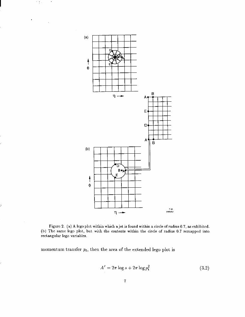
With the above definition of a jet, we may expect the population within the

circle of radius 0.7 to be nonuniform, and in fact similar to the fixed target popu-

lation of Fig. l(a). It is natural, therefore, to introduce polar coordinates within

the circle of radius 0.7 [Fig. 2(a)]. And, as before, it is again natural to remap

those polar coordinates into rectangular coordinates [Fig. 2(b)]. In this composite

phase-space the population of produced particles should be, within statistical fluc-

tuations, fairly uniform-provided there are no additional jets in either the original

lego plot or the extension we have created, and provided the pt of the jet is large

enough for a “central plateau” region to exist.

In a normal pp collision the area of the lego plot (i.e. the region populated by

the produced particles in a generic, “minimum-bias” event) is approximately

A=2nlogs. (34

If a pair of jets appear in the final state corresponding to a hard collision with

6

(b)

Figure 2. (a) A lego plot within which a jet is found within a circle of radius 0.7, as exhibited. (b) The same lego plot, but with the contents within the circle of radius 0.7 remapped into rectangular lego variables.

momentum transfer pt, then the area of the extended lego plot is

A’ = 2rlogs + 2alogp; (3.2)

7

and the multiplicity of produced particles grows accordingly.

In &CD, extra gluons of lower pt scales can also be radiated. This provides

new populations of jets which again extend the entire lego plot, including the

extensions we have exhibited. The self-similar character of this extension should

be evident. This gives rise to a phase-space area with a fractal dimension. The

total area will depend on the “resolution,” i.e. the value of minimum pt chosen.

We do not follow the mathematics of this here, much of which can be found in

the series of Lund papers [2]. If the minimum pt scale is chosen to be roughly

where ordinary hadronization takes over and below which observable jet structure

is at best obscure and at worst nonexistent, then once all jets with pt exceeding the

minimum value have been included, we expect the population of produced particles

in the extended phase space so generated to be reasonably smooth.

4. Some Kinematics

Before continuing this discussion, let us review a few kinematic facts of life.

These will help in resolving the aforementioned question of separating overlapping

jets and of distinguishing those properties of the picture we have introduced which

have an invariant meaning from those which depend upon the frame of reference

used. These ideas are best exhibited in examples drawn from eSe- physics, rather

than hadron-hadron collisions. The two points we make, quite elementary, are

that a rotation of coordinates can (1) create “kinematic” jets and (2) expand or

contract the “size”, as seen in the lego plot, of real jets.

We first consider the classic two-jet final state for the process e+e- + qq, as

seen in a variety of coordinate frames.:

8

f 2x

1

UN

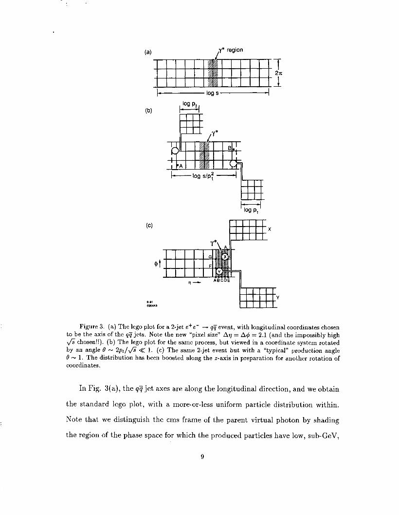
Figure 3. (a) The lego plot for a 2-jet e+e- + qq event, with longitudinal coordinates chosen to be the axis of the qij jets. Note the new “pixel size” An = AQ = 2.1 (and the impossibly high fi chosen!!). (b) The lego plot for the same process, but viewed in a coordinate system rotated by an angle 0 - 2~44 << 1. (c) Th e same 2-jet event but with a “typical” production angle 0 - 1. The distribution has been boosted along the r-axis in preparation for another rotation of coordinates.

In Fig. 3(a), the qij jet axes are along the longitudinal direction, and we obtain

the standard lego plot, with a more-or-less uniform particle distribution within.

Note that we distinguish the ems frame of the parent virtual photon by shading

the region of the phase space for which the produced particles have low, sub-GeV,

9

momentum in that frame. This has an invariant meaning, and can be useful in

more complicated situations to be described in what follows.

In Fig. 3(b), we have rotated coordinates by an angle

2Pt d=-<l G

(4.1)

and we see two “jets” at the edge of the longitudinal phase space. Note that the

longitudinal phase space has shrunk from an original length e - logs to a new

length

&logs-2logpt. (4.2)

This is compensated by the phase space, - 210g pt, contained within the jets

(circles of radius 0.7). This differs from the examples given in Section 3, which

extended the total phase-space area. Here a coordinate-rotation should not (and

does not) affect the physics.

It is interesting that if one draws, as shown, tangents to the circles of radius

0.7, they serve as a quite practical definition of the boundary of the phase space.

That is, if one estimates (Appendix 1) the mean number of particles (n) leaking

to the outside, the answer is

(n) = ie-2R (f) = $ (T) (4.3)

where R = 0.7 is the radius of the circle defining the jet, and dN/dq is evaluated

for the rapidity at the center of the circle; in our case 77 M log ,/T/pt.

Evidently if there is a stray particle on the outside, it will preferentially be

found at an azimuthal angle $ near that of the “jet.” Likewise there will be a

10

depletion within the “allowed” phase space in the azimuthal directions opposite to

those of the jets [points A and B in Fig. 3(b)]. Th is will be discussed further in

the context of the “string-effect” in Section 8.

In Fig. 3(c), we have rotated coordinates further to a “typical” value, so

that the separation Aq of the two jets is =S 2 units. We have also boosted the

configuration along the z axis into a “fixed-target” geometry-although this change

is not very noticeable at this point, due to the simple transformation properties of

the lego variables under the boost.

However, having made the boost, we again consider a rotation of coordinates.

The effect is best seen by first mapping the distribution into polar coordinates [Fig.

4(a)] and then making a small rotation-which simply amounts to a translation of

axes in Fig. 4(a).

Once the translation has been made [Figs. 4(b), 4(c)], polar coordinates may

be re-introduced and the map to lego variables performed. Depending upon the

magnitude of the rotation, we may end up again with a two-jet configuration,

overlapping jets [Fig. 5(a)], or a single jet [Fig. 5(b)]. This latter configuration

is what one would expect if one had fixed target kinematics (positrons incident

on atomic electrons) and a stupid choice of z-axis, i.e. one not along the beam

direction.

The example of overlapping jets in Fig. 5(a) is especially instructive. It shows

that even when jet products overlap in the lego plot they need not overlap intrinsi-

cally (although they occasionally will). A n d a way to resolve the ambiguity when it

occurs is to first make an appropriate longitudinal boost and to then make a simple,

small rotation of coordinates. The best choice is probably to rotate in such a way

that both jets shrink into a common circle-of-radius 0.7. Then, upon remapping

11

(a)

Circle of Radius 0. l-92

Figure 4. (a) The lego plot of Fig. 3(c) remapped into fixed-target polar coordinates. (b) The polar plot of Fig. 4( a a ) ft er a rotation of coordinates. The rotation angle is such that the jets X and Y overlap, i.e. have a separation of order 1. Notice that the circles defining the jet region have shrunk. (c) The same polar plot, but with a larger rotation angle, such that both jets X and Y shrink into a single circle-of-radius 0.7.

12

6-91 rl--, 6964A5

Figure 5. (a) The polar plot of Fig. 4(b) remapped into lego variables. The dashed lines show circles-of-radius 0.7 drawn around the jet cores X and Y, which have shrunk as a consequence of the coordinate-rotation. The circles of-radius 0.7 overlap, a situation best avoided by an additional coordinate rotation. Note we have chosen 4 = 0 at the center of the lego-plot in order to better display the jets. (b) The polar plot of Fig. 4( c remapped into lego variables. ) Essentially all collision products are now found within the circle-of-radius 0.7 shown.

the contents into lego variables, the two jets will in most cases be resolved.2

2 Another way is simply to choose a circle of radius R > 0.7 sufficient to contain all jet products, and then remap to polar coordinates. I am not sure which choice is to be preferred.

13

We also mention here a way of resolving the issue of how best to center the

circle-of-radius-O.7 surrounding a jet core. If the contents of the circle, when ex-

pressed in lego variables, have a leading “kinematic jet” [Fig. 3(b)], then the center

has been chosen unwisely. Any choice that does remove the leading “kinematic jet”

[Fig. 3(a)] may b e d eemed acceptable; i.e. the variation in such choices may be a

measure of the intrinsic uncertainty in determining the coordinates of the initiating

parton.

5. Plumbing

The lego-surface is periodic in 4, so that it really is the surface of a cylinder;

i.e. a pipe. From this point of view the addition of extra QCD jets to a collinear

two-jet lego plot, as in Fig. 3, simply amounts to cutting holes of radius 0.7 in

the pipe (which has in these units radius 1) and attaching new pipes to it, each of

length log pt (Fig. 6). L k i ewise the “kinematic jets” correspond to “elbows”-90

bends-in the pipe (Fig. 7). Th is collection of plumber’s fittings can be augmented

by “caps,” representing the leading-particle regions of phase-space at the ends of

the lego plot, regions which arguably ought to be left in polar coordinates rather

than being mapped into lego-variables (Fig. 8).

We now see that changes of coordinate systems can create or move elbows

in sections of pipe, without significantly changing their overall length, something

which, as mentioned in Section 4, is an intrinsic property. “Tees” and caps are

likewise intrinsic properties of the event as well. A “tee” represents a vertex where

a gluon was emitted, so it is labeled by an as(pf), with a reasonable estimate of

log pt being the length of the shortest section of pipe emergent from the tee.

14

7-91

6964A6

Figure 6. (a) The lego plot of Fig. 3(a) rolled up into a cylinder, or “pipe.” (b) A 2-jet event; the jet products are found on the surfaces of the new pipe segments.

One other type of plumber’s fitting, a connection or sleeve, is appropriate for

marking a specific region on a pipe (piece of lego plot). We encountered already

such a case in e+e- + q?j, where the shaded rapidity region (Fig. 3), which exhibits

the frame in which the initial state virtual photon is at rest, is an intrinsic property

of the event structure and is useful to mark.

There evidently are also generalized “tees” corresponding to vertices where two

or more gluon jets emerge form the same region of phase space. These are relatively

rare and will be neglected in what follows.

15

Figure 7. A plumber’s view of the “kinematic jets” of Fig. 3(b), generated by a small coordinate rotation from Fig. 6(a) [or 3(a)].

Fragmentation region “Cap”

(a)

’ Fragmentation “cap”

6-91 (b) 6964A6

Figure 8. (a) “Caps” attached to the ends of the lego plot, intended to cover the leading- particle, fragmentation region. (b) A plumber’s view of Fig. 8(a).

16

6. QCD Leading Logs: Decorating the Plumbing

For a given event, the basic architecture will be defined by the configuration of

the highest-pt jets, i.e. the pieces of pipe of greatest length. The generic e+e- + q?j

event we discussed has two pieces of pipe of length log &, connected by a y* (or

2) “sleeve,” which marks the e+e- ems frame.

7-91

6964A9

Figure 9. A plumber’s view of a “Mercedes” 3-jet final state in e+e- + qqg.

In most cases no additional QCD jet will have pt - fi. But occasionally

there will be “Mercedes” 3-jet events, where the junction “tee” occurs at the y*

“sleeve” (Fig. 9). But whatever the structure at the highest pt scale is, we may

then expect a “decoration” of the

The probability

quark line is [4]

per unit rapidity

9 in “leading log”

basic structure from lower-pt gluon (or qq) jets.

of finding an extra jet of scale pt attached to a

approximation

dP N 34P,2) dP,2 dq- 2n J-* P:

(64

So until the scale is quite low, not too many will occur.

One must “decorate” from the highest pt scales to the lowest. That is, one

breaks up the pt range into intervals. Starting with the highest pt which is relevant,

17

one appends the pieces of pipe of length log pt. Then one goes down in scale and

adds the shorter lengths to the entire structure. As already mentioned in Section 2,

this will generate an architecture for this plumbing which is fractal. The procedure

will terminate (as far as perturbative QCD is concerned) when the pipes to be

added have no significant length, but are all cap. At the lowest pt scale, one then

has to somehow address the physics of hadronization. The net result, however,

should be a quite uniform distribution of particles over the entire structure of

plumbing generated perturbatively.

7. QCD Coherence Effects: Coloring the Plumbing

Amplitudes for radiation of QCD jets must obey the rules of “color-coherence,”

or “angle-ordering” [5] , and it is appropriate here to describe (without derivation)

what it means in this language. We consider for definiteness the process e+e- +

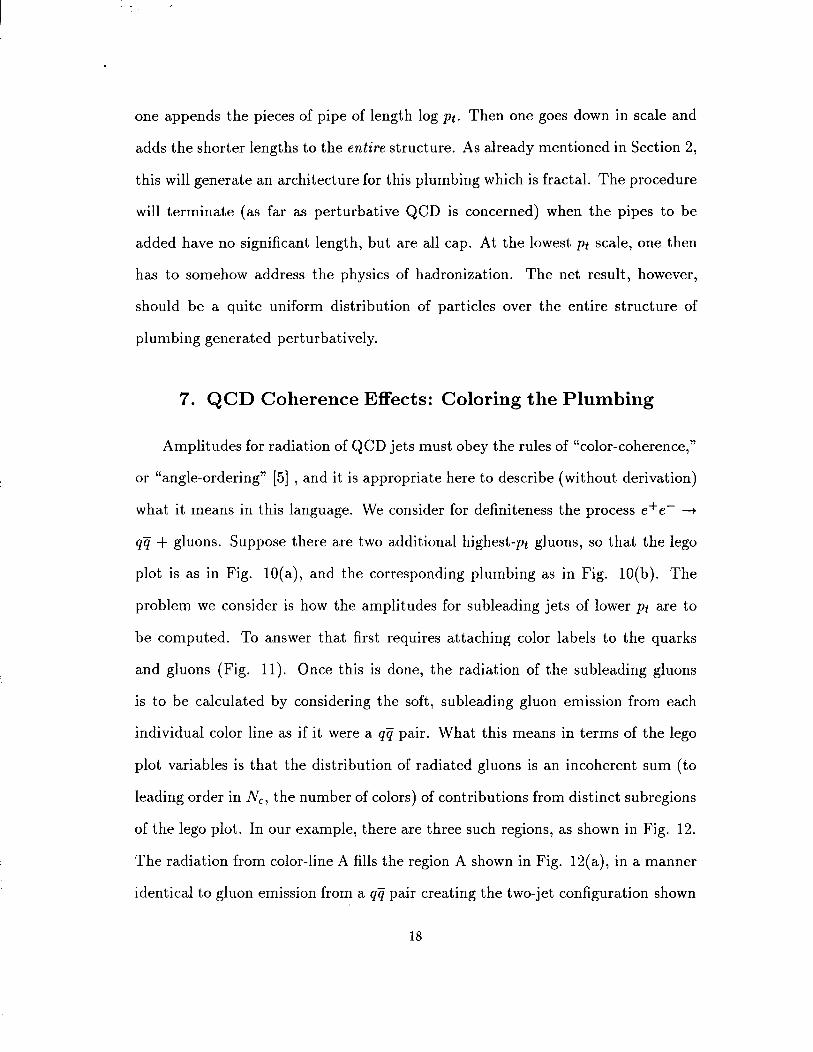
q?j + gluons. Suppose there are two additional highest-pt gluons, so that the lego

plot is as in Fig. 10(a), and the corresponding plumbing as in Fig. 10(b). The

problem we consider is how the amplitudes for subleading jets of lower pt are to

be computed. To answer that first requires attaching color labels to the quarks

and gluons (Fig. 11). 0 nce this is done, the radiation of the subleading gluons

is to be calculated by considering the soft, subleading gluon emission from each

individual color line as if it were a qij pair. What this means in terms of the lego

plot variables is that the distribution of radiated gluons is an incoherent sum (to

leading order in N,, the number of colors) of contributions from distinct subregions

of the lego plot. In our example, there are three such regions, as shown in Fig. 12.

The radiation from color-line A fills the region A shown in Fig. 12(a), in a manner

identical to gluon emission from a q?j pair creating the two-jet configuration shown

18

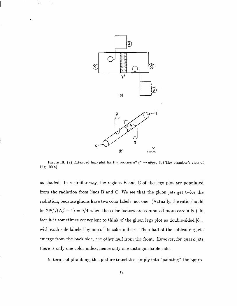
Figure 10. (a) Extended lego plot for the process e+e- + qijgg. (b) The plumber’s view of Fig. 10(a).

as shaded. In a similar way, the regions B and C of the lego plot are populated

from the radiation from lines B and C. We see that the gluon jets get twice the

radiation, because gluons have two color labels, not one. (Actually, the ratio should

be 2Nz/(Nz - 1) = 9/4 when th e color factors are computed more carefully.) In

fact it is sometimes convenient to think of the gluon lego plot as double-sided [6] ,

with each side labeled by one of its color indices. Then half of the subleading jets

emerge from the back side, the other half from the front. However, for quark jets

there is only one color index, hence only one distinguishable side.

In terms of plumbing, this picture translates simply into “painting” the appro-

19

(a)

4

A e+ e-

7.91 6964All

Figure 11. (a) Feynman diagram for the process e+e- + qqgg, with color labels attached to the lines. (b) Schematic of the color flow.

priate surfaces of the pipes with the appropriate color, A, B, . . ., in accordance

with the amplitude for the process. Emission of subleading jets from these sur-

faces is then an incoherent sum of gluon emissions from each section of plumbing

labeled by a given color index. Since any such subsystem is essentially a set of pipe

segments connected effectively by elbows, an easy way to determine the gluon ra-

diation from a given subsystem is to carry out a sequence of Lorentz-boosts which

straighten out the bends in that subsystem, leaving effectively a straight section of

20

(a)

(b)

6.91

6964A12

Figure 12. (a) Regions of phase space for which subleading gluons may be emitted from the leading quark lines. (b) R g e ion of phase space from which subleading gluons can be radiated from the virtual quarks produced by the y* .

pipe. The decoration of subleading jets onto that subsystem is identical to deco-

rating subleading gluons onto a collinear qij pair. [Of course once such a subleading

gluon is radiated, the lego surface must be “repainted” appropriately.]

There is, to be sure, some ambiguity on how to decorate elbows and tees. But

21

probably the most consistent rule is to perform the decoration of a subsystem in

its collinear reference frame as suggested above (i.e. in a frame where the plumbing

painted with the subsystem color index is a straight pipe). We shall give an example

of how this works in Section 8, where the “string effect” in S-jet production is

discussed.

In all this discussion, we again emphasize that the decoration process must

proceed from high-pt jets to low, so that the full fractal structure of the phase

space is created. Because of the running of CX~, it is mainly low-pt minijets which

will be the predominant feature generated by this process.

8. An Example: The “String Effect” in e+e- -+ 3 Jets

The processes e+e- t q?jg and e+e- -P qq-y have provided a classic example of

QCD coherence effects. [7] . W e h ere review the phenomenon in qualitative terms

from our point of view. What we will compare is the particle density emitted

opposite to each of the jets. This can be defined in a precise way, by specifying in

all cases a reference frame in which the remaining two jets are collinear.

Start with the process e+e- + qq-y and first estimate the particle production

opposite the y. The lego-plot is shown in Fig. 13 and the particle density is to be

computed at point A. Clearly this is just d2N/dq d4 for an ordinary e+e- + qq

event.

More interesting is to compute the density opposite the q jet in the frame in

which y and q are collinear. The lego plot is shown in Fig. 14, and the plumbing

is essentially an “elbow” as far as hadron emission is concerned, since we have

just boosted the uniform two-jet distribution seen in Fig. 13 to a different Lorentz

frame.

22

(4

Figure 13. (a) Lego plot for the process e+e- + qijy in a reference frame in which the qij pair is collinear. (b) A plumber’s view of Fig. 13(a).

To estimate the density at the base of the “elbow,” point B, it is convenient

to boost to a fixed target frame of reference and remap the configuration in polar

coordinates (Fig. 15). Th e d ensity at point B is just what one gets by extending

the lego variables centered around the q jet core into the remainder of the phase

space, since in this frame there is just a collinear jet configuration with axis in

that direction. What now needs to be done is to compare in the neighborhood of

point B this measure with the lego-plot measure centered about the 7-q jet axis.

This is just the area of the shaded sector versus the area of the cross-hatched one.

The ratio is about l/4. Hence we conclude that the particle density opposite the

q jet (in this collinear frame) is about 25% of the density opposite the photon jet

(in the qq collinear frame). In passing we note that the density expected in the

“forbidden” region of the lego plot, i.e. the region to the left of the tangent CD

in Fig. 14(a) is quite small since it corresponds to the region interior. to the circle

CDE in Fig. 15, which covers only 50% of a unit of A7 A$ as measured from the

23

Y*

(a)

c-

9 (W

7-91

6964A14

Figure 14. (a) The lego plot for e+e- + qij-y in a reference frame in which the yij pair is collinear. (b) A plumber’s view of Fig. 14(a).

q-jet axis. This qualitative result is made more quantitative in the appendix.

It is now straightforward to consider the process e+e- -+ qifs. Given the color

labeling shown in the Feynman diagram in Fig. 16, we paint the surfaces of the

lego-plumbing as shown in Fig. 17. Figure 17(a) is appropriate to consideration of

the particle density opposite the gluon jet where we see [Fig. 18(a)] a net depletion

of - 50% relative to the densities in the rest of the qQ jets. In Fig. 17(b), however,

where the kinematics is appropriate to the distribution opposite the if (or q) jet we

see an enhancement of 25% relative to what is expected in the quark jet. This is

the “string effect,” expected theoretically and seen experimentally.

24

0.7 x 0.7 Leg0 unit referenced lo y-q-axis

0.7 x 0.7 Leg0 unit referenced to q jet

Jet axisv

Figure 15. The lego plot of Fig. 14 remapped into polar coordinates after a large boost in the z-direction.

Figure 16. Color labels for the process e+e- -+ qijg.

9. Hadron-Hadron Collisions: “Hole Fragmentation”

In hadron-hadron collisions there is always the preferred axis of the incident

beams which provides the natural coordinate system for laying out the lego vari-

25

64

Figure 17. (a) C 1 fl o or ow in the lego plot for the process e+e- ---+ qqg in a collinear qij frame. (b) Color flow in the lego plot for the process e+e- + qqg in a collinear gij frame.

ables. In general, the analysis parallels what we have already discussed. Here

we only mention one additional feature, of importance because the initial-state

partons responsible for the hard collisions carry color. Initial-state color leads to

initial-state gluon radiation, and it is appropriate to describe its properties in the

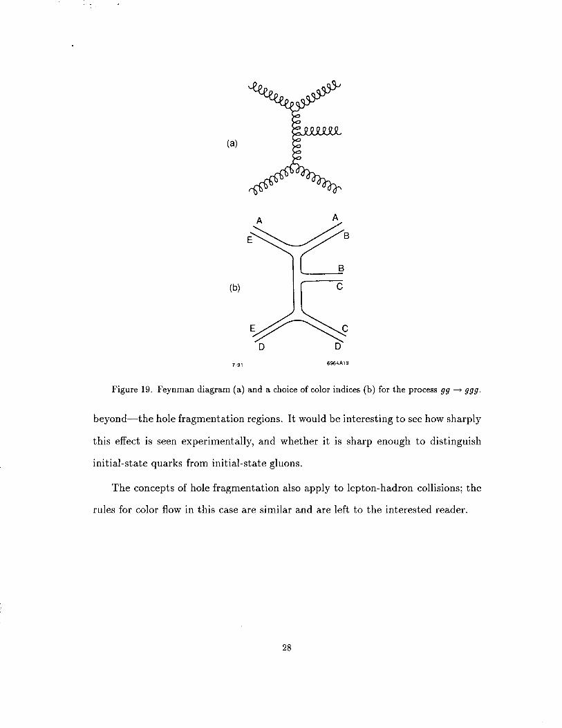
language we have introduced. Suppose for definiteness the process is gg + ggg,

with color indices labeled as shown in Fig. 19. The incident initial-state gluons

are usually specified to have a definite longitudinal momentum pa = xpbeam, and a

“small,” usually unspecified, transverse momentum pt. Once the pt is specified, say

0.7 GeV within a factor two, the initial-state rapidities of the incident gluons can

be estimated within an uncertainty of order f 0.7. We mark these regions of the

phase-space as “hole-fragmentation” regions, since in the collision those initial-state

partons are abruptly transported to some distant region of phase space, thereby

requiring some special final-state hadronization to occur in their original region of

phase space [8] .

The “color-dipole” rules of leading-log perturbative QCD may now be applied

26

(4

t Jet ‘Core 8-9, 6964A18

Figure 18. (a) Rapidity distribution of particles produced opposite the gluon jet in e+e- + qqg, as seen in a collinear q?j reference frame. (b) Rapidity distribution of particles produced opposite a q jet in e+e- + qijg, as seen in a collinear gq reference frame.

in a straightforward way. The extended lego plot is shown in Fig. 20, with the

rules for coloring the surfaces shown. Then the process of decoration of the phase

space with softer jets, minijets, and hadrons, as described in previous sections may

proceed as before.

In a high-pt binary gluon-gluon collision, there is predicted to be consider-

able extra multiplicity along the beam-jet directions, extending out to-but not

27

(a)

03

7-91 6964Al9

Figure 19. Feynman diagram (a) and a choice of color indices (b) for the process gg + ggg.

beyond-the hole fragmentation regions. It would be interesting to see how sharply

this effect is seen experimentally, and whether it is sharp enough to distinguish

initial-state quarks from initial-state gluons.

The concepts of hole fragmentation also apply to lepton-hadron collisions; the

rules for color flow in this case are similar and are left to the interested reader.

28

Hole

tl

Hole

8-91 b 6964A20

Figure 20. (a) Lego plot for gg + ggg. The “hole” fragmentation regions mark the estimated rapidities of the initial-state gluons. (b) Rules for “coloring” the lego plot for determining emission of subleading gluons, in accordance with the choice of color indices shown in Fig. 19(b).

29

10. Conclusions

Of what use is all this? We believe that the variables we have used are a practi-

cal tool for describing complex event structures containing jets in terms of (fractal)

extensions of the phase space, and also that the definition of jet that is used is suf-

ficiently precise to be a very practical one. The problem of distinguishing distinct

jets which overlap when viewed in the usual lego variables may be resolvable using

the flexibility in choosing coordinates, as described in Section 4. The description

appears to be eminently suited for visual computer displays of event structure, and

we hope that someone expert in software development might pick this idea up.

Important here is our emphasis on individual particles, and not on transverse-

momentum flow. There is a need to display distributions of “entropy” (particle-

numbers) as well as “energy” (transverse-momenta); these are complementary con-

cepts. Also noteworthy is the need for very good resolution in Aq and A$ of indi-

vidual hadrons (and photons) in order to delineate accurately the populations in

the extended phase space.

This work was stimulated in large part [9] by consideration of the physics

associated with a full-acceptance detector for SSC-scale proton-proton collisions. A

prime goal of such a detector, or any other having broad rapidity acceptance, should

be the perception and classification of patterns or morphologies of individual events

which have considerable complexity. One’s choice of coordinates or descriptive

elements is for such applications crucial. We believe the choice made here has

much virtue and is worth pursuing.

I thank A. Giovannini for encouragement and my colleagues at SLAC, espe-

cially Vittorio Del Duca and Philip Burrows, for useful discussions on this material.

30

APPENDIX

Consider the process e+e- + qq, with th e jets produced at a small angle 6

relative to the e+e- collision axis:

2Pt 6=-<l. lb-

(A-1)

Define the “kinematic jets” as the contents of the circle of radius 0.7 surrounding

the jet axes as seen in the lego-plot referenced to the e+e- beam directions. Then

draw tangents in the lego plot to those circles as shown in Fig. 3(b) [the dashed

lines]. We are interested here in how many produced particles leak to the region

exterior to the phase space bounded by those tangents. We assume pt >> 1 GeV

and also assume, in a frame of reference with z axis aligned along the jets, that the

relevant secondary hadrons are produced with a flat rapidity distribution. However

we work hereafter in the frame referenced to the eSe- beam directions.

The four-momentum of the primary quark is

and the four-momentum of a secondary hadron will be

(A-2)

64.3)

with

k; = (O,Ak,z) (A4

expected to be on average no more than 1 GeV. The longitudinal momentum Ak is

chosen such that e2 = 0. What we really need are the rapidities of primary quark

31

and secondary hadron, which are

qqnark = f en PO + ” = en if PO - Pz Pt

qhadron = +?n------ e. + ez = en -e. - e,

en

In order that the hadron rapidity exceed the jet rapidity by an amount R (the

radius of the circle defining the jet contents: R = 0.7), we must have

(?‘hadron - r]jet )=[n

or

I’~+~[ -R ISI <e * (A.7)

The condition in Eq. (A.7) can only be satisfied if

1x1 1 - eAR < ~ IGI

< 1 + eeR

(A4

(A4

and only then for a limited set of relative orientations. For a given magnitude of

32

kt and z, the geometry is shown in Fig. 21. We see that the azimuthal angle 4

7-21 6964A21

Figure 21. Geometry for the calculation of leakage into the rapidity-gap.

must be less than a value $0 which, to reasonable approximation, is given by the

expression

~2 = (4FwR)2 - (ZIZI - q2 0

IGil 121 * WY

For fixed Izl we may therefore estimate the “leakage” AN to be

(A.lO)

Here z = I~l/lF& and the integration only goes over values of the variable for

which the square root is positive. Since kt disappears from the estimate, we may

33

average over all values of kt. Finally, in the limit of large R the formula simplifies

with the substitution y = 1 + we -R. The result is, approximately,

(A.11)

which is what was quoted in Eq. (4.3).

A more complete analysis is straightforward, but is best done directly via Monte

Carlo simulations.

34

REFERENCES

[l] For a good review, see H. Harari, Proceedings of the 14th Scottish Univer-

sities Summer School in Physics (1973), ed. R. Crawford and R. Jennings,

Academic Press (N.Y.), 1974, p. 297.

[2] B. Andersson, P. Dahlqvist, and G. Gustafsson, Phys. Letts. B214, 604

(1988). A recent discussion is given by G. Gustafsson, Lund preprint, LU

TP 90-16 (N ovember 1990).

[3] Essentially this definition is advocated by J. Huth et al., Fermilab preprint

FERMILAB-CONF 90-249-E.

[4] See for example Ref. 2 for more details.

[5] Y. Azimov, Yu. Dokshitzer, V. Khoze, and S. Troyan, Phys. Lett. B165, 147

(1985).

[6] This idea goes back to G. Veneziano, Nuovo Cimento m, 190 (1968).

[7] For reviews see G. Gustafsson, Lund preprint LU TP 90-17 (November 1990),

and V. Khoze, CERN preprint CERN-TH 5849 (September 1990).

[8] J. Bjorken, Phys. Rev. D7, 2747 (1973). See also J. Bjorken, Journal de

Physique Cl, Suppl. 10, Vol. 34, 385 (1973).

[9] J. Bjorken, Expresion of interest to the SSC (EoI-19), SLAC-PUB-5545, to

be published in the Proceedings of the Sixth J. A. Suieca Summer School:

Particles and Fields, Campos do Jordao, Brazil (January 1991), ed. 0. Eboli.

35