Skewed Idiosyncratic Income Risk overthe Business Cycle: Sources and Insurance∗

Christopher Busch† David Domeij‡ Fatih Guvenen§

Rocio Madera¶

May 18, 2020

Abstract

Recent studies have shown that idiosyncratic labor income risk becomes moreleft-skewed during recessions. This procyclical skewness arises from a combi-nation of higher downside risk and lower chances of upward surprises duringrecessions. While this much is known, some important open questions remain.For example, how robust are these patterns across countries that differ in theirinstitutions and policies, as well as across genders, education groups, and oc-cupations, among others? What is the contribution of wages versus hours toprocyclical skewness of earnings changes? To what extent can skewness fluc-tuations in individual earnings be smoothed within households or with govern-ment policies? Using panel data from the United States, Germany, Sweden,and France, we find four main results. First, the skewness of individual incomegrowth (before-tax/transfer) is procyclical while its variance is flat and acyclicalin all three countries. Second, this result holds even for full-time workers con-tinuously employed in the same establishment, indicating that the hours marginis not the main driver; additional analyses of hours and wages confirm thatboth margins are important. Third, within-household smoothing does not seemeffective at mitigating skewness fluctuations. Fourth, tax-and-transfer policiesblunt some of the largest declines in incomes, reducing procyclical fluctuationsin skewness.Keywords: Idiosyncratic income risk, skewness, countercyclical risk.

∗For helpful comments, we thank Nick Bloom, Alexander Ludwig, Kurt Mitman, Luigi Pistaferri, Anthony Smith,and Kjetil Storesletten, as well as seminar and conference participants at various institutions. Busch acknowledgesfinancial support from ERC Advanced Grant (Agreement no. 324048 “APMPAL”) and from the Spanish Ministryof Economy and Competitiveness, through the Severo Ochoa Programme for Centres of Excellence in R&D. Domeijacknowledges financial support from the Jan Wallander and Tom Hedelius Foundation. Guvenen acknowledges financialsupport from the National Science Foundation.

†UAB, MOVE, and Barcelona GSE; chris.busch@movebarcelona.eu; www.chrisbusch.eu‡Stockholm School of Economics; david.domeij@hhs.se; https://sites.google.com/view/daviddomeij/§University of Minnesota, FRB Minneapolis, and NBER; guvenen@umn.edu; www.fatihguvenen.com¶Southern Methodist University; romadera@smu.edu; www.rocio-madera.com

1 IntroductionRecent empirical studies have shown that idiosyncratic labor income risk becomes

more left-skewed during recessions. This rise in left-skewness arises from a combinationof larger downside risks and smaller upward surprises during recessions. Put differently,the center of the earnings change distribution remains quite stable over the businesscycle, whereas the upper tail compresses and lower tail expands in recessions and viceversa in expansions, resulting in procyclical skewness fluctuations. A striking exampleof this phenomenon could be seen during the Great Recession: between 2007 and 2009,the average decline in the labor earnings of US men was almost 7%—the largest two-year decline since the Great Depression—whereas the median change in labor earningswas +0.1%—slightly positive. The large mean decline was entirely driven by the upperand lower tails collapsing during those two years as opposed to a negative aggregateshock pulling down the entire earnings distribution (Guvenen, Ozkan and Song (2014)).Therefore, skewness fluctuations can potentially matter both at the micro level (i.e.,the idiosyncratic risk faced by workers) and the macro level (for understanding thebehavior of aggregates).

While the procyclical skewness of earnings changes has been well documented, someimportant questions naturally raised by these new facts remain open. In this paper,we aim to shed light on four of these related questions. First, how robust are thesepatterns across countries—which differ in their institutions and policies—as well asacross genders, education groups, and occupations, among others? Second, what isthe contribution of hourly wages versus hours worked to the procyclical skewness ofearnings changes? Third, to what extent are households able to smooth the skew-ness fluctuations in the earnings growth of each spouse, thereby mitigating the effecton the household’s consumption and welfare? Fourth, and finally, how effective aregovernment social insurance policies (i.e., the tax-and-transfer systems) in smoothingskewness fluctuations over the business cycle?

To address these questions, we use five panel datasets on earnings histories fromfour different countries, which collectively provide the information necessary for theempirical analysis. The bulk of our analysis focuses on three countries—the UnitedStates, Germany, and Sweden—which differ in important dimensions relevant for ouranalysis, such as household structures, the tax-and-transfer systems, and labor marketinstitutions, among others. The datasets we use are based on Social Security records(the Sample of Integrated Labour Market Biographies, or SIAB, for Germany), tax

1

register data (the Longitudinal Individual Data Base, or LINDA, for Sweden), andhousehold surveys (the Panel Study of Income Dynamics, PSID, for the United Statesand the German Socio-Economic Panel, SOEP for Germany), covering more than threedecades in each country. We complement the main analysis with another administrativepanel dataset from France (Declaration Annuelle des Donnees Sociales, DADS), whichhas more detailed information on hours and wages, allowing us to shed more light onthe relative contribution of each to the skewness fluctuations in earnings changes.

Our analysis yields four results. First, starting with before-tax-and-transfer (“gross”)individual earnings growth, we find that skewness is robustly procyclical in all threecountries, with substantial fluctuations from peak to trough. In fact, if anything, thefluctuations are larger in Sweden and Germany compared with the United States. Togive one example, the skewness of individual earnings growth in Germany went from0.31 in 1990, the peak year before the start of a deep recession, to –0.28 in 1994 (thetrough), using the Kelley skewness measure which is a robust and convenient statistic(Figure 3). Put differently, these figures imply that, in 1990, the gap between the 90thpercentile and the median (hereafter, P90–P50) of the earnings growth distributionwas twice as large as the gap between the median and the 10th percentile (P50–P10),whereas this ratio had completely flipped by 1994, with the lower tail (P50–P10) grow-ing to twice the size of the P90–P50 by 1994 (using eq. (2) below). The changes werejust as large for Sweden. In contrast to these large swings in skewness, the varianceof earnings growth is mostly flat and acyclical—not countercyclical as it was typicallymodeled in the earlier literature.

These findings both confirm the empirical evidence found by Guvenen et al. (2014)from US administrative data and show that they hold more broadly—in administrativedata from two other developed economies, as well as in survey data (the PSID andSOEP). In addition, we show that this result is robust across sub-populations definedby gender, education, occupation, and private/public sector employment. Moreover,the cyclicality of skewness also holds for five-year income changes, which shows thatthe procyclical swings in skewness is present in the persistent component of earnings.

Second, we find that changes in hours and wages are both critical in generatingthe procyclical skewness in earning changes. We establish this result in several ways.Starting with Germany, while the SIAB dataset does not report work hours, dailywages can be calculated for full-time workers. Using this information, we can focuson full-time workers who are also continuously employed at the same establishment,a subsample where many potential sources of variation in hours and wages are either

2

absent or much more limited (e.g., unemployment, large drops in hours, changes inwages due to job changes, among others). Even for these strongly-attached workers,changes in daily wages is robustly procyclical, whereas the variance continues to beacyclical. We find the same result for Sweden by merging in extra information fromLISA, a separate administrative database.

While these results clearly show that skewness fluctuations are not primarily drivenby the hours margin, they pertain to full-time workers and there is no continuousmeasure of hours to study its cyclicality directly.1 Thus, to bring more direct evidencewe use the DADS, based on French Social Security records, which reports informationon work hours and wages for all workers. We find that changes in both wages and hoursare strongly procyclical with similar magnitudes to each other (Table III). Lookingat subsamples, in the sample of strongly-attached workers (same as defined above),procyclical skewness is almost entirely driven by changes in wages, with the skewnessof hours changes showing no cyclicality. The pattern is partially reversed for the restof the baseline sample, for whom skewness is procyclical for changes in both wagesand hours, but the latter is twice as volatile as the former. Collectively, these separatestrands of evidence all point to procyclical skewness as a robust property of fluctuationsin changes in individual earnings, wages, and hours.

Third, moving from individual earnings to household earnings, we did not findany evidence indicating that households are able to mitigate the higher in downsiderisk during recessions in each spouse’s individual earnings. For example, comparing thecyclicality of the earnings growth of actual households to synthetic households that areformed by randomly pairing unrelated men and women shows that the procyclicalityof skewness is not any lower for actual households. We have also studied the responseof spousal earnings to changes in the head’s earnings to see if there was any evidencethat the larger downside risk and smaller upside surprises in recessions triggered astronger spousal response. We have not found evidence of such a response despiteexamining households across the entire earnings distribution and earnings changesacross the distribution. This is not completely surprising given that spouses are facingthe same labor market conditions as the heads during recessions, so they are likely tohave difficulty increasing their work hours or finding a second job.

Fourth, moving from gross to disposable (or post-government) household income,1The PSID and the SIAB are not suitable for the purposes of this analysis because teasing out

the cyclicality of the skewness of changes in a variable essentially involves triple-differencing the data,which exacerbates the measurement error in reported hours in survey data (which is a more severeproblem for hours than annual earnings—see Bound et al. (2001) for evidence from validation studies).

3

we find that the tax-and transfer system reduces the procyclicality of skewness in allthree economies. In the United States and Sweden, the elasticity of Kelley skewnesswith respect to GDP growth is about half as large for the post-government householdearnings measure compared with its pre-government counterpart. However, this similareffect on skewness in the two countries are driven by different sources: In the UnitedStates, the tax-and-transfer system mainly reduces the cyclicality of the lower tail,whereas the opposite is true in Sweden—the major effect is on the upper tail, whichbecomes acyclical, with a smaller effect on the lower tail.2 We also unbundle thecomponents of the tax-and-transfer system and find differences in the effectivenessof each component in each country. Overall, we conclude that the tax-and-transfersystem plays an important role in reducing the magnitude of procyclical fluctuationsin the skewness for households. Our analysis does not address the costs of the tax-and-transfer system, which should clearly be weighed against any potential benefit.Furthermore, the reduced procyclicality of skewness in some cases comes from thereduced procyclicality of the upper tail, partly achieved through progressive taxation.

We have also examined the extent of business cycle fluctuations in the fourth mo-ment—the kurtosis—of earnings changes but did not find large and robust cyclicalpatterns. That said, one aspect of kurtosis matters greatly for evaluating the effects ofskewness fluctuations. Basically, earnings changes are highly leptokurtic—they havelong and fat tails—which interact with, and amplify, the effects of skewness fluctua-tions to generate a large rise in idiosyncratic risk in recessions.

The paper is organized as follows. The next section discusses the data sources, andSection 3 describes the empirical approach. Section 4 presents the results for grossindividual income for the three countries. Section 5 zooms in on various groups inthe population, and presents the results on the wages versus hours margin. Section 6expands the analysis to households and post-tax-transfer income. Section 7 concludes.

Related LiteratureEarlier empirical work in the literature was limited by the small sample size and

time span of the available survey-based panel datasets, such as the PSID, leadingresearchers to make parametric assumptions to obtain identification. One common

2As we discuss further in Section 6.2, the results for Germany were mixed. On the one hand, in theSOEP data, the skewness of post-government household earnings changes is essentially acyclical. Onthe other hand, the SOEP data also shows some important differences from SIAB data in cyclicalitypatterns for individuals, which raises some uncertainty about the reliability of this result for Germany.

4

assumption is that shocks to earnings are Gaussian, which implies zero skewness. Re-stricting attention to the changes in the mean and variance of income shocks, Storeslet-ten, Telmer and Yaron (2004) concluded that the variance of income shocks in the USdata is countercyclical.3

Guvenen et al. (2014) revisit this question using a large panel data set on theearnings histories of US males from SSA records. The large sample size allowed themto relax parametric assumptions as well as to examine variations in skewness. Theyfound that the variance of income shocks is stable over the business cycle and is robustlyacyclical, whereas the skewness of shocks varies significantly over time in a procyclicalfashion. The current paper goes substantially beyond their analysis by studying twonew countries and four datasets, shedding light on the contribution on hours versuswages, moving beyond before-tax-and-transfer individual earnings to analyze householdearnings with various levels of government provided social insurance, among others.

Busch and Ludwig (2020) adapt the parametric approach of Storesletten et al.(2004) to allow for skewness fluctuations and analyze the cyclicality of labor incomerisk in the United States. They come to the same substantial conclusion as we do,namely, that variation of income risk over the business cycle is asymmetric. In ongoingwork, Angelopoulos, Lazarakis and Malley (2019) follow the approach in the presentpaper to study the cyclicality of higher-order risk in the United Kingdom using paneldata from the British Household Panel Survey. They confirm the same finding ofstrongly procyclical skewness for the UK since the early 1990s. Similarly, Harmenbergand Sievertsen (2018) document procyclical skewness of individual earnings changesin administrative Danish data. In a recent paper, Pruitt and Turner (2018) analyzeindividual and household-level income dynamics using United States tax records fromthe IRS. They also document procyclical skewness of income changes for both male andhousehold incomes. Unlike in our four datasets, they find countercyclical dispersion ofmale (not household) earnings growth.

A couple of recent papers aim at exploring the role played by hours versus wages forthe observed cyclical dynamics of earnings changes. In an analysis of administrativeunemployment insurance data fromWashington State, Kurman and McEntarfer (2017)document procyclical skewness of hourly wage changes. They also explicitly show thatthe share of workers realizing a wage cut increases substantially in recessions. Pora

3Using a similar approach, Bayer and Juessen (2012) studied the cyclicality of the variance inGermany, the UK, and the US, and different patterns in Germany and the UK relative to the US andattributed it to differences in institutions.

5

and Wilner (2017) document in French administrative data that the distribution ofearnings changes was more negatively skewed in the 2008 recession than in the directlypreceding period. Conditioning on income, they find that for high-income workers,hourly wages account for this change of the distribution, while for low-income workershours worked are more important. Blass-Hoffman and Malacrino (2016) study datafrom Italian workers and find the employment margin to play an important role indriving skewness fluctuations in earnings.

Finally, our paper also contributes to a growing literature on the skewness in workerand firm outcomes (beyond labor earnings), such as in firm employment growth (e.g.,Decker, Haltiwanger, Jarmin and Miranda (2015), Ilut, Kehrig and Schneider (2018),and Salgado, Guvenen and Bloom (2019)), firm productivity (Kehrig (2011) and Sal-gado et al. (2019)) and stock returns (e.g., Oh and Wachter (2018), and Ferreira (2018),and many others).

A growing number of theoretical and quantitative studies emphasizes the impor-tance of the skewness and kurtosis of income shocks for various questions. In assetpricing, some studies found that the procyclical skewness of consumption and incomegrowth helps explain some puzzling features of asset prices (Mankiw (1986), Constan-tinides and Ghosh (2014), Schmidt (2016)). Recent research on monetary and fiscalpolicy also emphasizes the role of higher-order income risk in shaping optimal policyor in modifying the standard channels through which policy works. Examples includeKaplan, Moll and Violante (2016) who examine the monetary transmission mechanismin the presence of leptokurtic shocks, and Golosov, Troshkin and Tsyvinski (2016)who find that, in a Mirleesian setting, the optimal tax schedule is greatly affected bywhether or not one accounts for higher order moments of income shocks.

2 The DataThis section provides an overview of the datasets we use in our empirical analy-

sis, the sample selection criteria, and the variables used in the subsequent empiricalanalyses. Further details can be found in Appendix A. Briefly, we employ four paneldatasets corresponding to three different countries: the Panel Study of Income Dy-namics (PSID) for the United States, covering 1976 to 2010;4 the Sample of Integrated

4The PSID contains information since 1967. We choose our benchmark sample to start in 1976because of the poor coverage of income transfers before the 1977 wave. We complement our resultsusing a longer period whenever possible and pertinent.

6

Labour Market Biographies (SIAB5) and the German Socio-Economic Panel (SOEP)for Germany, covering 1976 to 2010 and 1984 to 2011, respectively; and the Longitudi-nal Individual Data Base (LINDA) for Sweden, covering 1979 to 2010. The PSID andthe SOEP are survey-based datasets. The PSID has a yearly sample of approximately2,000 households in the core sample, which is representative of the US population; theSOEP started with about 10,000 individuals (or 5,000 households) in 1984 and, afterseveral refreshments, covers about 18,000 individuals (10,500 households) in 2011.6

The SIAB is based on administrative social security records and our initial samplecovers on average 370,000 individuals per year. It excludes civil servants, students,and self-employed workers, which make up about 20% of the workforce. From theperspective of our analysis, the SIAB has two caveats: (i) income is top-coded at thelimit of income subject to social security contributions, and (ii) individuals cannotbe linked to each other, which prohibits identification of households. We deal with(i) by fitting a Pareto distribution to the upper tail of the wage distribution7 andwith (ii) by using data from SOEP for all household-level analyses. Throughout theanalysis, we focus on West Germany, which for simplicity we refer to as Germany.LINDA is compiled from administrative sources (the Income Register) and tracks arepresentative sample with approximately 300,000 individuals per year. In addition,for some of the analysis of individual level income dynamics we use the LongitudinalIntegrated Database for Health Insurance and Labour Market Studies (LISA), whichcovers the Swedish population of 16 years and older individuals. In it we are able toidentify annual workplace information. Furthermore, we back up the individual levelanalysis of earnings dynamics for full-time workers using additional data for 1995–2015from French social security records, the Declaration Annuelle des Donnees Sociales(DADS), which is described in the appendix.

The measure of labor earnings we use is meant to be comprehensive to the extentallowed by each dataset. In all cases, it includes wage and salary income (inclusive ofbonuses, overtime, paid time off, and so on) plus the labor portion of self employment

5We use the factually anonymous scientific use file SIAB-R7510, which is a 2% draw from theIntegrated Employment Biographies data of the Institute for Employment Research (IAB).

6These numbers refer to observations after cleaning but before sample selection. Only the repre-sentative SRC sample is considered in the PSID. The immigrant sample and high-income sample ofthe SOEP are not used, because they cover only subperiods.

7The imputation is done separately for each year by subgroups defined by age and gender. Forworkers with imputed wages, across years, we preserve the relative ranking within the age-specificcross-sectional wage distribution. The procedure follows Daly et al. (2014); see Appendix A.4 fordetails.

7

income. The earnings measure from SIAB does not include self employment incomebecause the dataset lacks information on it. More details of each variable can be foundin the data Appendix A.

For each country, we consider three samples: two at the individual level—onefor males and one for females—and one at the household level. The samples areconstructed as revolving panels: for a given statistic computed based on the timedifference between years t− s and t, the panel contains individuals who are ages 25 to59 in periods t− s and t (s = 1 in the case of Sweden and Germany, and s = 2 in thecase of the United States) and have yearly labor earnings above a minimum thresholdin both years. Imposing this threshold allows us to exclude individuals with very weaklabor market attachment during the year and also avoids problems with zeroes whendealing with logarithms as we will see below. The threshold is set to the earnings levelthat corresponds to 520 hours of employment at half the legal minimum wage, whichis about $1,885 US dollars for the United States in 2010.8 To avoid possible outliers,we exclude the top 1% of earnings observations in the PSID and SOEP, but not inLINDA (which is from administrative sources). For each individual, we record age,gender, education, and gross labor earnings. By gross earnings we mean a worker’scompensation from his/her employer before any kind of government intervention in theform of taxes or transfers.

Furthermore, the SIAB provides time-consistent occupational codes based on theKldB-88, the 1988 version of the classification of occupations by the German FederalEmployment Agency. In parts of the analysis of individual income dynamics, we useinformation on 30 occupational categories, which are listed in Appendix I for reference.

The household sample is constructed by imposing the same criteria on the house-hold head and adding specific requirements at the household level. More specifically, ahousehold is included in our sample if it has at least two adult members, one of thembeing the household head,9 that satisfy the age criterion and household income thatsatisfies the income criteria. At the household level, we analyze pre- and post govern-ment earnings. Pre-government earnings is defined as the sum of gross labor earnings

8For the United States, we use the federal minimum wage. There is no official minimum wagein Sweden or Germany during this period. For Germany, we follow Fuchs-Schündeln et al. (2010)and take a minimum threshold of 3 euros (in year 2000 euros) for the hourly wage. For Sweden, theeffective hourly minimum wage via labor market agreements was around SEK 75 in 2004 (Skedinger,2007). For other years, we adjust the minimum wage using the growth rate in the mean real wages.

9In PSID and SOEP, the head of a household is defined within the dataset. In LINDA, the headof a household is defined as the sampled male.

8

earned by the adults in the household. Post-government earnings is constructed byadding taxes and transfers.

3 Empirical ApproachFollowing the recent literature on higher-order risk discussed above, our empirical

approach is nonparametric and flexible. To analyze dynamics, we focus on incomechanges between two periods and analyze the behavior of this distribution over thebusiness cycle. Specifically, we compute moments m [∆syt], where yt ≡ logYt is thenatural log of individual income, Yt, and ∆syt ≡ yt − yt−s is the change or growthrate between years t − s and t. 10 For Germany and Sweden, we consider s = 1 and5 corresponding to short- and long-run changes, respectively. Starting with the 1997wave, the PSID switches to a biennial structure, so we use s = 2 instead of s = 1 forthe United States through the entire sample period.11

Our primary measures for volatility and skewness are quantile-based, which haveimportant advantages over standardized moments (variance and the skewness coeffi-cient). Some of these advantages are substantive—more below—whereas others aretechnical or practical: they are more robust to outliers; they allow scrutinizing differ-ent parts of the distribution by varying the quantiles used; and they are often easierto interpret than the values of standardized moments. The specific moments we focuson are the log differential between the 90th and 10th percentiles (L9010) as a measureof dispersion, dispersion in the upper (L9050) and lower (L5010) tails, and the Kelleymeasure of skewness defined as follows:

Sk =(P90− P50)− (P50− P10)

(P90− P10). (1)

The Kelley measure of skewness has a simple interpretation. It measures the dif-ference between the fraction of the overall dispersion, L9010, that is in the right tail,L9050, and the fraction that is in the left tail, L5010. Rearranging (1) gives a simplemapping from a a given Kelley value into the fraction of overall dispersion that is in

10We repeat the main analysis in this paper using the arc-percent measure of growth, 2(Yt −Yt−s)/(Yt + Yt−s), which allows us to drop the minimum threshold requirement described above andinclude observations with zero income in either t or t − s. This makes no substantive effect on theconclusions we report in this paper.

11We calculate overlapping s-year differences up to ∆sy1996, and non-overlapping s-year differencesfrom then and up to ∆sy2010, for s = 2, 4.

9

the right tail:P90− P50

P90− P10= 0.5 +

Sk

2, (2)

which is not possible to do with the skewness coefficient. A second advantage of Kelleyas noted above is that it does not suffer from the extreme sensitivity to outliers thatthe skewness coefficient does. Kim and White (2004) provide a cautionary analysisshowing that the skewness coefficient can reveal spurious relationships due to outliersfound in some commonly used datasets. This is especially relevant for the survey datafrom PSID and SOEP that we use in our analysis.

There is also a more substantive benefit of studying quantiles directly: it can reveala simpler underlying empirical structure or can uncover patterns that are obscuredwhen we focus too closely on standardized moments. Two examples—which will turnout to be empirically relevant—can help illustrate these points. In the first case,suppose that a common negative shock hits all the workers who would have been in thebottom 20% of the income growth distribution, thereby reducing P20 and all percentilesbelow, leaving the rest of the distribution unchanged. This would register as a rise inthe variance but it is not coming from a symmetric expansion of the distribution whichis customarily associated with a higher variance. Instead, it is directly related to thedistribution becoming more left-skewed, without any increase in higher percentiles.

For the second example, suppose that the same negative shock in the first examplehits not only the bottom 20% but also the top 20% of the income growth distribution,reducing all percentiles below P20 and above P80, without affecting the percentilesbetween P20 and P80. In this case, the variance may very well remain unchanged(notice that L9010, L8020, etc., are already constant) but skewness actually becomesmore negative. Even though this situation entails a large change in the distribution anda large increase in risk, the variance would not give a hint about this. Furthermore, ifwe were to describe the changes in the distribution in terms of standardized moments,we would characterize it as a negative shock to the first moment (the mean will falleven though the median is constant), no shock to the second moments, and a negativeshock to the third moment. This description obscures the fact that there was actuallyonly one shock that hit both tails in the same direction, and what looked like threeseparate shocks to three moments—the fall in the mean and skewness and the constantvariance—are actually all the consequence of this one tail shock.

10

Defining Business CyclesWe use two main indicators for business cycles. The first one is based on the

official classification of peaks and troughs by the National Bureau of Economic Research(NBER) for the United States and by the Economic Cycle Research Institute (ECRI)for Sweden and Germany.12 It is well known, however, that some key macroeconomicvariables do not perfectly synchronize with expansions and contractions, but theirfluctuations might still have an impact on earnings. For example, the US stock marketexperienced a significant drop in 1987, officially classified as an expansion year, andindeed the skewness of household income growth dips in that year (Figure 2a). Otherexamples (e.g., 1996) are easy to find for Germany and Sweden. To better capture thesemore continuous changes in aggregate conditions, we use the (natural) log growth rateof GDP over s years—∆s(logGDPt) ≡ log(GDP t) − log(GDP t−s) and regress eachmoment m on a constant, a linear time trend, and this indicator of business cycles:

m (∆syt) = α + γt+ βm ×∆s(logGDPt) + ut. (3)

The key parameter of interest is βm, which measures the cyclicality of moment m.For a quantitative interpretation of the results reported in the next sections, Figure 1reports annual log GDP growth for each country.

4 Empirical Results: Before-Tax Individual Income

We start our empirical analysis with labor income at the individual level, measuredbefore taxes and government transfers. This is the same income measure used in recentwork that found the skewness of the US income growth distribution to be volatile andprocyclical and its dispersion to be flat and acyclical (e.g., Guvenen et al. (2014)). Inthis section, we ask three questions that are left unanswered by this earlier work.

First, we ask if these cyclical features are specific to the United States or whetherthey are robust features of business cycles that are also observed in other countrieswhose labor markets differ greatly from that in the US. To give an example of these

12We make two adjustments to NBER and ECRI classifications. For the US, we classify the1980–1983 period as a single “double-dip” recession instead of two separate ones. For Sweden, un-like ECRI, we classify the 2001–2003 period as a recession because Swedish GDP fell by a similarmagnitude to that in the US and Germany during these years, as seen in Figure 1.

11

Figure 1: Annual log GPD Growth: US, Germany, and Sweden

Note: The figure plots log GDP growth for each country. The shaded areas indicate US recessions. The numbers inparentheses next to each country indicate the standard deviation of the short-run GDP growth series over the period1976-2010, where short-run is one-year difference for Germany and Sweden, and two-year difference for the UnitedStates, to be consistent with the timing of the PSID data used in our analysis. The corresponding number for the one-year change in the United States is 2.8%. The series for Germany corresponds to West Germany up to and includingthe 1990–91 change and to (unified) Germany from 1991–92 on.

differences, consider the fact that only 10.7% of US workers are unionized and only11.9% are covered by trade union agreements, whereas the corresponding fractionsare 18.1% and 57.6%, respectively, in Germany, and 67.3% and 89%, respectively, inSweden.13

A second question we ask is whether the patterns of cyclicality found by Guvenenet al. (2014) using US administrative earnings data from the Social Security Adminis-tration (SSA) are also borne out in the PSID (survey data), which is widely used in theanalysis of income dynamics. The answer is less than obvious because earlier papersthat used the PSID and adopted a Gaussian parametric econometric model (which re-stricts the skewness to zero) found a strongly countercyclical variance of shocks (e.g.,Storesletten et al. (2004)). This raises the question: is it the differences in the datasetsor in the methodologies (or both) that accounts for these different conclusions? Byremoving parametric restrictions, our analysis can shed light on this question.

Finally, because of the limited number of covariates available in the SSA data,Guvenen et al. (2014) were not able to explore potential variation in the cyclicalitypatterns by gender, education, occupation, private versus public sector employees,

13OECD (2016). The reported numbers are for 2013.

12

among others, which we address starting in this section.

4.1 Cyclicality of Variance and SkewnessWe begin in Figure 2 with a simple time-series plot of the standard deviation and

the skewness coefficient of the short-run income change distribution for male workers inthe United States (biennial), Germany (annual) and Sweden (annual).14 We start withstandardized moments because of their familiarity before we delve into the analysisof quantiles. Recessions are indicated as shaded areas. Two key patterns are clearlyevident here. First, in all three countries, the standard deviation varies little overtime and the small fluctuations it displays do not typically comove with the businesscycle. In contrast, the skewness coefficient shows significant procyclical fluctuations,with skewness dipping consistently in recessions and recovering in expansions. Hence,Figure 2 provides a visual confirmation of the procyclical skewness/flat dispersionpattern in both US Survey data as well as in Germany and Sweden.

Next, to quantify the degree of cyclicality and compare it across countries, weuse the regression framework described above in (3). Table I reports the cyclicalitycoefficient, βm, for four quantile-based moments—L9010, Kelley Skewness, L9050, andL5010—separately for each gender and the three countries.15 Starting with the UnitedStates, the coefficient on L9010 is quantitatively small, slightly negative for men andslightly positive for women, and statistically insignificant with t-stats less than 1.4for both genders. These estimates confirm the acyclicality of dispersion in the UnitedStates that we saw in Figure 2. The same acyclicality is also seen in the bottomtwo panels for Germany and Sweden with small point estimates that are statisticallyinsignificant.16

Cyclicality of Skewness

We next turn to the cyclical behavior of skewness. Starting with Figure 3 (leftpanels), the Kelley skewness for males shows the same procyclical pattern as the skew-

14The skewness coefficient of random variable x is the third standardized moment:E (x− E [x])

3/σ3, where σ is the standard deviation.

15We ran two alternative versions of these regressions and obtained the same substantive results.First, we used the arc-percent change rather than log change of income to capture the extensivemargin—or zeroes in income (Table C.1 in Appendix C.1). Second, we use a dummy for recessionsas a business cycle indicator rather than log GDP change, in the regression (Table C.2 in AppendixC.2). In both cases, we find the same substantive patterns described here.

16All regression results in the paper based on SIAB data are robust to various sensitivity checks weconducted to address issues of topcoding and a structural break in the wage variable. See AppendixF for details.

13

Figure 2: Standard Deviation and Skewness of Short-Run Income Growth: Males

(a) United States (b) Sweden

(c) Germany (SIAB)

Note: Linear trend removed, centered at sample average. Shaded areas indicate recessionary periods(see footnote 12). Year denotes ending year in the growth rate calculations.

ness coefficient in Figure 2, which is probably not surprising but still reassuring.17 Inthe PSID, Kelley skewness drops significantly during the 1980s double-dip recession,falling from 0.15 for the 1979–80 change to below –0.2 for the 1982–83 change, as wellas the two recessions in the 21st century. There is no drop in skewness during the early1990s recession, which may be due to potential data issues during the transition PSIDwent through from 1992 to 1993 or it may be due to the somewhat unusual timing ofthis recession which appears as two dips in economic activity and skewness in the SSAdata analyzed by Guvenen et al. (2014).

The synchronization between Kelley skewness and the business cycles is even clearer17To reduce the number of figures for readability, we have moved the analogous figure for females

to the appendix

14

Table I: Cyclicality of Log Annual Income Change Moments: Before-Tax/TransferIndividual Income

L9010 Kelley L9050 L5010United States

Males –0.54 2.25 0.68 –1.23(–1.38) (4.79) (2.49) (–4.27)

Females 0.40 1.17 0.86 –0.47(1.39) (3.01) (2.57) (–2.38)

SwedenMales –0.26 3.64 0.78 –1.04

(–0.64) (3.94) (4.51) (–2.50)

Females 0.33 1.77 0.65 –0.32(1.84) (2.64) (2.91) (–1.99)

Germany (SIAB)Males 0.15 5.48 0.95 –0.80

(0.36) (5.80) (3.14) (–4.11)

Females 0.34 2.55 0.80 –0.46(0.48) (2.05) (1.25) (–1.80)

Note: Each cell reports the cyclicality coefficient βm (on log GDP change) in a regression of themoment specified in the column header on log GDP change plus a constant and a time trend (eq. 3).Newey-West t-statistics are in parentheses.

in Sweden and Germany (middle and bottom left panels of Figure 3). In particular,Kelley skewness falls significantly during the early 1990s recession, which was muchdeeper in these countries compared with the United States. In Germany, the Kelleymeasure swung from 0.31 in 1989–90 down to –0.28 in 1993–94, implying a dramaticshift in the length of the tails: Whereas the upper tail (L9050) accounted for two-thirds(0.5+0.31/2≈ 0.66) of the overall L9010 gap in the 1989–90 period, with the remainingone-third accounted for by the lower tail (L5010), these ratios completely flipped by theend of the recession (1993–94), with L5010 growing to account for almost two-thirds(64%) and L9050 shrinking to one-third of L9010. Notice that Kelley skewness fallsfrom 1995 to 1996, which is technically an expansion year for Germany but the GDPgrowth did in fact fall between those years (see Figure 1). Finally, Sweden experienceda similar but slightly smaller drop with the Kelley going from 0.08 to –0.31 between

15

the same two years (with the share of the lower half, L5010 rising from 46% to 66%).

In Table I, the cyclicality coefficients for males in column 2 are all positive andstatistically significant at the 0.1% level, confirming the strong procyclicality of Kelleyskewness. The estimated βKelley for males is 2.25 for the US, 3.64 for Sweden, and5.48 for Germany, implying a 2.5-fold larger fall in Kelley in Germany than in the USfor the same 1% slowdown in GDP growth. This result is somewhat surprising giventhe higher prevalence of unions and other worker protection measures in Germany andSweden relative to the United States, so we will analyze it in greater detail in the nextsection.18

To give a quantitative interpretation to these coefficients, consider a two standarddeviation decline in log GDP growth in Sweden, swinging from one standard deviationabove average to one standard deviation below, which represents a moderate recession.With the estimated βKelley = 3.64, Kelley skewness will fall by 3.64×(2×0.0236) ≈ 0.17.For the sake of discussion, if the upper tail to lower tail ratio was 50/50 in an expansion,it would fall to 42/58 in a recession. A severe recession with a four standard deviationswing in GDP growth (such as the 1990–1993 period) would bring the upper-to-lowertail ratio from 50/50 to 33/67. These are very large changes in the relative size ofeach tail over just a few years, especially in a country like Sweden whose institutionsare geared toward social insurance.19 Finally, skewness is also procyclical for femaleworkers in all countries, with positive and statistically significant coefficients for Swedenand the US at 1% level, and for Germany at 5% level.

4.2 Inspecting the TailsSkewness can become more negative from either the compression of the right tail or

the expansion of the left tail or both. Each tail is informative about different aspectsof labor market outcomes: for example, the compression in the right tail could resultfrom a decline in upward moving opportunities (smaller wage gains with promotionsor job changes), whereas the expansion in the left tail is likely to result from largerdownside risk (higher likelihood of job losses, increased duration of unemployment,and so on). Furthermore, the government policies that we study below have differenteffects on each tail. All of these lead to the question: What is the contribution of eachtail to the procyclical fluctuations in skewness? And how does this contribution varyacross these three countries?

18Running the regression with the skewness coefficient instead of Kelley measure yields very similarresults.

19The corresponding changes in Sk for the U.S and Germany are 0.15 and 0.22, respectively.

16

Figure 3: L9010, Skewness, and Tails of Short-Run Income Growth: All Males

(a) United States (b) United States

(c) Sweden (d) Sweden

(e) Germany (SIAB) (f) Germany (SIAB)

Note: Linear trend removed, centered at sample average. Shaded areas indicate recessionary periods(see footnote 12). Horizontal gray line in the right axis of the left panel indicates zero (symmetry)reference line. Year denotes ending year in the growth rate calculations.

17

The right panels in Figure 3 plot L9050 and L5010 over time. While the magni-tudes somewhat differ, in all three countries both tails contribute significantly to theprocyclical skewness. In particular, L9050 starts falling while L5010 starts rising rightaround the beginning of the recession and they reverse the roles with the start of theexpansion. The last two columns of Table I report the cyclicality coefficients for thetwo tails, which are positive for L9050 and negative for L5010, confirming the patternwe see in Figure 3. The statistical significance of the estimated coefficients is fairlyhigh for men (t-stats between 2.49 and 4.51) and somewhat lower but still significantfor women (ranging from 1.80 to 2.91, with the exception of L9050 in Germany with at-stat of 1.25).

Another point to notice in Table I is that, for all countries, the estimated β’sfor each tail are of similar magnitudes to each other. For example, for Sweden, thecoefficient for L9050 is 0.78 and for L5010 it is –1.04. The corresponding coefficientsare 0.68 and –1.23 for the US, and 0.95 and –0.80 for Germany. Thus, the shrinking ofone tail is largely offset by the expansion of the other tail, making total dispersion, theL9010, move very little over the cycle. As a result, skewness becomes more negative inrecessions without any significant change in the variance. One partial exception is alsoilluminating: L9010 rises slightly during the 1990s recession in Sweden and Germany(less so in the US) because the left tail expands more than the right tail contracts. So,the rise in dispersion is in fact due to a change that is mostly asymmetric in nature,which would not have been apparent by focusing on the variance alone.

These new insights and more nuanced interpretations of income risk over the busi-ness cycle underscore the importance of the finer-grain analysis through quantiles un-dertaken here compared with the simpler analysis of a few standardized moments. Inparticular, interpreting changes in the variance without considering the changes inskewness delivers an incomplete picture that can be highly misleading.

Turning to the estimates for females in Table I, we observe the same patterns ofcyclicality as those of men, whenever the coefficient is significant. In particular, L9050is procyclical for the US and Sweden, whereas L5010 is countercyclical for all threeeconomies (though only significant at the 10% level for Germany). That said, themagnitudes of coefficients are smaller for women, especially for Kelley skewness, whichis largely driven by the much smaller coefficients on L5010 compared with men (about1/3 that of men’s in the US and Sweden and about 1/2 in Germany). In other words,compared with men, the right tail compresses during recession in a comparable fashion,whereas the expansion of the lower tail–or the rise in downside risk—is much smaller.

18

We will return to this finding when we analyze households earnings.

4.3 Persistence of Skewness FluctuationsIt is well understood that the economic implications of transitory income changes

are very different from those of persistent changes. Hence, a natural question is theextent to which the procyclical fluctuations in skewness pertain to the persistent com-ponent of earnings. To fix ideas, consider the standard permanent-transitory model ofearnings dynamics:

yt = zt + εt

zt = zt−1 + ηt

where ηt and εt are zero-mean disturbances, and zt and εt represent the permanent andtransitory components, respectively. The s-year difference of log income is yt − yt−s =

Σsj=1ηt−j + εt − εt−s,which contains s permanent innovations and always 2 transitory

ones, so longer-term changes increasingly reflect the properties of permanent shocks.Thus, to investigate the persistence of skewness fluctuations, in this section we studyfive-year changes for Germany and Sweden and, given the biennial nature of the PSIDafter 1997, four-year changes for the United States. That said, regressions that useoverlapping long-term changes face serious econometric problems in sample sizes foundin time series data.20

With these issues in mind, we use more transparent graphical constructs to an-alyze the properties of persistent changes. Starting in Figure 4, each panel shows ascatterplot of either L9010 or Kelley skewness of longer-run earnings changes for malesagainst five-year log GDP growth. The patterns are fairly easy to discern. For Swedenand Germany, the scatterplots of L9010 are clouds showing no evident relationshipwith GDP growth as confirmed by the flat fitted line. For the United States, thereis some evidence of a downward slope, which is partly attributable to the outlier onthe left top corner. The scatterplots for Kelley skewness reveal a stronger positive

20For example, if five-year changes are computed for every year of the sample, the overlap betweenobservations induce strong serial correlation, which makes the autocorrelation consistent standarderrors of coefficients to be downward biased, inflating the significance of estimates coefficients (e.g.,Richardson and Stock (1989)). This can be an empirically serious problem, for example as hasbeen recognized in the literature on stock return predictability regressions (e.g., Kirby (1997) andreferences therein). Using only non-overlapping observations reduces the already modest sample sizedramatically. We did estimate the cyclicality regressions using five-year changes and found the samepatterns but do not include them because of the concerns outlined here.

19

Figure 4: Cyclicality of Dispersion and Skewness of Long-Run Income Changes, Males:United States, Sweden, and Germany (SIAB)

(a) United States (b) United States

(c) Sweden (d) Sweden

(e) Germany (f) Germany

Note: Each figure is a scatterplot of either the L9010 or Kelley skewness of five-year earnings changeagainst five-year log GDP change (four-year change used for the United States).

20

relationship with GDP growth, which is especially strong in Sweden and Germany.21

Appendix G shows the same figures for women, which are again qualitatively tellingthe same story. It also shows the time-series of moments of five-year income changes.

Additional Evidence from Sub-Populations

We bring additional evidence on the persistence of skewness fluctuations by recog-nizing that time series data on the entire population is also panel data on subpopu-lations, and in this particular case, on occupational groups. We conduct this analysisusing the SIAB dataset from Germany, the other datasets are either too small to allowthis finer grain analysis (the PSID and SOEP) or lack information on occupations (inour version of LINDA)

In SIAB, we assign each worker to one of 30 occupational categories in year t basedon their occupation in t − 5. We compute the same moments of five-year changes asbefore but now individually for each occupation group. We also construct a businesscycle indicator for each occupation by taking the five-year change in average earningsin that occupation. The top left panel of Figure 5 shows the scatterplot of L9010for each occupation-year cell against average earnings growth for the same cell, whichbasically shows no relationship, confirming the acyclical nature of dispersion foundabove. In contrast, the scatter plots for Kelley skewness in the top right panel showsa very clear upward pattern, with substantial range of variation in the magnitude ofKelley skewness (in the y-axis). The bottom two panels make clear that both tails areindividually strongly cyclical with L9050 showing a somewhat larger range of variationover the occupation-specific cycle than L5010.

These conclusions are not sensitive to using occupation-specific cycles. Table G.1in Appendix G reports the raw correlations of each moment with five-year aggregateGDP growth. For Kelley skewness the correlations are all positive, with a correlationof 0.49 even at the 10th percentile of correlations. In contrast, the correlations forL9010 range from –0.35 at the 10th percentile to 0.29 at the 90th percentiles with amedian of –0.12.

Overall, these findings corroborate our main results by showing that the same21In an earlier draft of this paper, we have also estimated a more formal econometric process for

earnings dynamics featuring permanent and transitory shocks, targeting a large number of momentsof short- and long-run earnings changes. The estimated process revealed a strong procyclical variationin the skewness of the permanent component. Similarly, Busch and Ludwig (2020) estimate earningsprocesses using moments of the cross-sectional income distribution, allowing for state-dependent dis-tributions of income shocks. They find systematic variation of cross-sectional skewness, which can beattributed to procyclical skewness of the persistent component.

21

Figure 5: Distribution of Five-Year Income Growth; Occupation-Specific Cycles(SIAB): Males

(a) Males, L9010 (b) Males, Kelley’s skewness

(c) Males, L9050 (d) Males, L5010

Note: Scatterplot of moments of five-year earnings change against occupation-specific average incomegrowth over the same horizon. There are 900 data points: 30 five-year changes for 30 occupationseach.

patterns we observed in the aggregate economy hold, more strongly, at the more dis-aggregated level. The patterns for females look qualitatively the same; see AppendixG for details.

5 Digging Deeper into the Main FindingsIn this section, we extend our analysis of individual earnings in two directions.

First, we examine the robustness of our findings in different subgroups of the popu-lation, defined by educational attainment, by private/public sector employment, and

22

occupation. Second, we ask the degree to which the procyclical fluctuations in skewnessare explained by changes in hours worked or to changes in wages, or both.

5.1 Heterogeneity across Groups of WorkersEducation and Public vs. Private Sector

We begin by classifying workers (separately for each gender) by educational attain-ment (college versus non-college graduates) and, separately, by whether they hold aprivate- or public-sector job. The share of male workers who are college educated is12%, 16%, and 25%, respectively, in Germany, Sweden, and the United States (theanalogous numbers for women are 8%, 17% and 25%). Differences in the size of pub-lic sector employment are even larger and also vary significantly between men andwomen.22 Moreover, public sector jobs are often thought of as less risky, offering gen-erous employment protection and less volatile compensation, so it is interesting to askif this perception is actually borne out in the data.

To avoid producing too many different figures, we pool the statistics from the threecountries as follows: For a given group, we first construct a statistic, say L9010, andlog GDP growth for each country-year pair, and assign the statistic to its correspond-ing quartile of the log GDP growth distribution (pooled over all years), and averagewithin each quartile. Figure 6 shows the L9010 and Kelley skewness for males. Thestandardization of moments and log GDP changes is performed independently for eachcountry before pooling across countries, which implies that a deviation from zero indi-cates a standardized deviation from the country-specific mean of the moment. For eachquartile, the bars correspond to the average moment for (ordered from the left) the fullsample, college graduates, non-college graduates, private employment, and public em-ployment, respectively. Figure 6 shows that the nature of income risk is qualitativelysimilar across all male subgroups: overall dispersion is acyclical (panel a), whereas Kel-ley skewness is strongly procyclical (panel b). Furthermore, as Figure B.1 in AppendixB shows, the upper tail is procyclical, and the lower tail is countercyclical. The resultsfor females look qualitatively the same (Figure B.2).

22For men, the share of public jobs is 23% in Sweden, and 10% and 13% in Germany and theUnited States. For women, the corresponding figures are 63%, 36% and 18%. For these statistics, wedefine public sector employment as jobs in public administration, health care, and education (sectorswhich in Germany and Sweden are dominated by public sector jobs or by jobs funded by the public).Historically, most workers in these sectors were employed by the public; this is less true today.

23

Figure 6: Higher-Order Moments by Quartiles of Log GDP Change: Males

(a) Dispersion (L9010) (b) Kelley skewness

Note: For different samples, each bar shows the average moment across years and countries by quartilesof log GDP change. Both log GDP changes and moments are standardized by country.

Occupational Groups

We return to the occupational groups in SIAB data for Germany, analyzed in thelast section, and focus on annual—rather than five year—changes, which allows us torun the cyclicality regression in (3) separately for each occupation without running intothe overlapping observations problem (see footnote 20). Figure 7 shows the estimatedβ’s for L9010 and Kelley skewness for each occupation. As seen in the bottom panel,the estimated β′s for Kelley skewness are positive for every occupation and statisticallysignificant for the vast majority of them. As before, β’s for dispersion are close to zerofor the vast majority of occupations and is not statistically significant for any of them.Further results for the upper and lower tails are in Appendix B.2.

5.2 Earnings versus WagesA workers’ earnings can change because of a change either in hourly wages or in

hours worked or a combination of both. So, an important question is to understandwhether the fluctuations in the skewness of earnings growth is driven by wages orhours or both. Reliable data on hours worked is scarce because it is often unavailablein administrative data sets (such as the US SSA data, which prevented Guvenen et al.(2014) from addressing this question) and measurement error in survey data is a moresevere problem for reported hours than for annual earnings (see Bound et al. (2001)for a review of evidence from validation studies). This problem is exacerbated by the

24

Figure 7: Dispersion and Skewness of Short-Run Income Growth by Occupation: Males(Germany (SIAB))

(a) Dispersion (L9010)

(b) Kelley skewness

Note: Separate regressions for each of 30 occupation segments. Each marker reports the coefficient onlog GDP change of a regression of a moment of the distribution of changes in an income measure onlog GDP change, a constant, and a linear time trend. The confidence bands are based on Newey-Weststandard errors (maximum lag length considered: 3).

25

fact that teasing out the cyclicality of the skewness of changes in a variable essentiallyinvolves triple-differencing the data, which amplifies the measurement error in theunderlying data.

In this section, we shed light on this question using SIAB for Germany and alsobringing additional evidence from two datasets that we did not use so far in the analysis.We start with SIAB, which contains information on the duration of each employmentspell and on whether it is a part-time or full-time job. Next, we perform a comparableanalysis for Sweden. In particular, we go beyond our baseline dataset LINDA andlook at the LISA dataset, which covers the whole population and which has a focuson individuals’ labor market experiences rather than on family and transfers. Ofmain relevance for our analysis is that it has workplace (establishment) information.Neither SIAB nor LISA contain direct information on hours worked. We thereforecomplement this analysis using French social security data (the DADS) from 1995 to2014, which contains hours worked for each employment spell as reported by employers(see Appendix D for a description of the data).

Full-Time Workers in Germany and Sweden

We first look at workers with stable employment relationships. To accommodatethe different structures of SIAB and LISA, we perform slightly different but comparableanalyses. In both datasets, we focus on subsamples of workers whose earnings dynamicsare not driven by changes in the extensive margin.

In the SIAB, we define a full-time worker if her full-time spells add up to at least50 weeks of employment in a given year. (A less strict definition of full-time workers as45 weeks of employment does not change the results.) The wage variable is the averagedaily wage rate, where the average is taken over all full-time spells during the year.This is the same measure used in Dustmann et al. (2009) and Card et al. (2013). Weconsider the annual change in the average daily wage rate of male workers who are inthe full-time sample in both years.

For completeness, the first row of Table II reproduces the estimated β’s for thebaseline sample from Table I. Row 2 reports the corresponding β’s using average dailywages for full-time workers instead of annual earnings of all workers. Notice howsimilar the coefficient on skewness is compared with the baseline sample in the firstrow (4.73 versus 5.48). Note that 88% of males (73% of women) are in the full-timesample.23 Naturally, the dispersion of earnings changes is wider than that of wage

23The sample of full-time female workers contains about 73% of women (who make up only 54%

26

Table II: Cyclicality of Log Annual Income Change Moments for Males: IndividualIncome vs. Daily Wages, Germany (SIAB) and Sweden (LISA)

L9010 Kelley L9050 L5010Germany

Earnings 0.15 5.48 0.95 –0.80(Baseline Sample) (0.36) (5.80) (3.14) (–4.11)

Daily Wages –0.09 4.73 0.30 –0.39(Full-Time Workers) (–0.54) (6.31) (3.77) (–3.20)

Daily Wages –0.12 4.98 0.28 –0.40(Establishment Stayers) (–0.81) (5.78) (3.29) (–3.20)

SwedenEarnings –0.06  3.64    0.87   –0.94(Baseline Sample) (–0.73)      (4.34)      (4.30)     (–3.81)

Earnings   –0.12    1.78    0.16   –0.28(Establishment Stayers) (–4.53)     (7.43)      (5.34)     (–7.90)

Note: Each cell reports the coefficient on log GDP change of a regression of a moment of the dis-tribution of changes in an income measure on log GDP change, a constant, and a linear time trend.Newey-West t-statistics are included in parentheses (maximum lag length considered: 3). Full-Timeare those that work full time for at least 50 weeks in both years for which the change is calculated.

changes, which is reflected by the point estimates on the tails (last two columns),which are about half as big for wage changes. In the third row, we further restrictthe sample by selecting workers who not only work full time but also work at least50 weeks at the same establishment in two consecutive years. For these workers notonly changes in hours but also changes in daily wages should be smaller than for theprevious sample.24 Perhaps surprisingly, the estimated β coefficients, including the oneon skewness (4.98), barely change.

For the question at hand, there are two shortcomings of LISA relative to SIAB.First, we cannot identify the duration of job spells in LISA, and second, we can onlylook at total annual earnings, not at daily wages. Still, we can select a sample of workers

of the observations) that contribute to the measures of earnings changes for women. The correspond-ing figures are 88% of individuals and 82% of observations for males. This implies that part-timeemployment plays a more important role for the female sample.

24The sample of full-time female workers that do not switch establishments contains about 61%of women (who make up about 40% of the observations) that contribute to the measures of earningschanges for women. The corresponding figures are 80% of individuals and 65% of observations formales.

27

with minimal room for the extensive margin of labor supply to affect their earningschanges. We do this by selecting workers who earn income from the same establishmentin four consecutive years, from t−2 to t+1, and have that establishment as their mainemployer in t− 1 and t. Clearly, this is a more selected group of stayers than the onein SIAB.

The second panel of Table II shows the corresponding estimation results for Sweden.The first row shows the estimates for the full population covered by LISA, which arevirtually identical to the estimates based on LINDA. The second row shows the resultsfor the workers staying at their establishment. The coefficient on skewness is abouthalf the size of row 1 but continues to be very significant. An intermediate conclusionis thus that the overall dynamics are not exclusively driven by the extensive marginin either Germany or Sweden. Taken together, this points in a similar direction asrecent evidence by Kurmann and McEntarfer (2019), who document in data fromWashington that during the Great Recession the incidence of nominal wage cuts forjob stayers increased substantially—accompanied by systematic reductions in hoursworked, which further decreases earnings.

Hours versus Wages: Additional Evidence from FranceWhile the spell data for Germany allows us to explore the roles of days worked

vs. changes in daily wages, part of the variation in daily wages can potentially beattributed to changing hours worked during the day. We thus consider those variablesseparately, using the same regression framework for France.25 Table III shows resultsfor earnings, hours, and hourly wage changes for males. First, earnings changes displaythe same patterns we have seen so far, with a cyclicality coefficient on Kelley skewnessthat is even higher (7.38) than any of the three other countries (Table I), while L9010is acyclical with small and statistically insignificant coefficients in column 1.

Second, as seen in the second and third rows, the skewness of both changes in hourlywages and hours worked display significant procyclicality with coefficients of 3.37 and4.27, respectively. However, one important difference between the two is seen in thetails: whereas the cyclicality coefficient for L9050 are similar for wages and hours (0.80and 0.72), the left tail of the wage growth distribution is much less countercyclical(–0.22) than that of hours (–1.02). This is consistent with the downward rigidity of

25Given the available data from the DADS, we use the years 1995–2015 in the analysis, which gives20 years for which we can estimate one-year changes. The standard deviation of log GDP growth overthat time period is 0.98%.

28

Table III: Cyclicality of Hours Worked vs. Hourly Wages; France (DADS): Males

L9010 Kelley L9050 L5010Baseline Sample

Earnings –0.28 7.38 1.37 –1.65(–0.58) (7.60) (4.27) (–5.4)

Hourly Wages 0.58 3.37 0.80 –0.22(1.55) (2.78) (2.49) (–1.2)

Hours Worked –0.3 4.27 0.72 –1.02(–0.57) (4.19) (5.04) (–2.23)

Subsample A: Full-Time, Establishment StayersEarnings –0.04 5.43 0.46 –0.50

(–0.14) (2.58) (1.79) (–2.28)

Hourly Wages 0.47 4.96 0.74 –0.27(1.35) (2.63) (2.15) (–1.83)

Hours Worked 0.47 –1.69 0.03 0.44(0.98) (-0.22) (0.11) (0.64)

Baseline Excluding Subsample AEarnings –0.23 4.63 2.94 –3.16

(–0.18) (5.55) (4.33) (–3.24)

Hourly Wages 0.4 2.33 0.77 –0.38(1.04) (2.40) (2.60) (–1.16)

Hours Worked –0.02 4.71 3.13 –3.15(–0.01) (5.93) (3.81) (–3.58)

Note: Each cell reports the coefficient on log GDP change of a regression of a moment of the distri-bution of changes in the indicated measure on log GDP change, a constant, and a linear time trend.Newey-West t-statistics are included in parentheses (maximum lag length considered: 3). Full-timeEstablishment Stayers are those workers working in Full-time employment for the same establishmentfor at least 50 weeks in both t− 1 and t. Baseline without Full-time are those workers who are not in50 weeks full-time employment in either t− 1 or t.

wages, making hours a more elastic margin to adjust for employers. Overall, thisevidence confirms that the procyclicality of skewness is driven both by wages andhours.

To gain further insights, we split the baseline sample into full-time workers that stayin the same establishment and the rest of the baseline sample. The results in the middle

29

and bottom panels of Table III. Earnings changes display strong procyclicality butslightly smaller than the baseline (βKelley = 5.43); however, almost all of it is now due towages (4.96) and almost none from hours (–1.69 and statistically insignificant). Resultsare partially flipped for for the rest of the sample in the bottom panel: the skewness ofearnings changes is still procyclical but now a larger component is coming from hours,which is both volatile and very cyclical (bottom row). Overall, the additional evidencefrom France confirms and complements our results from Germany and Sweden. Bothwages and hours play significant roles in generating skewness fluctuations in earnings.For more strongly attached workers, wages play a more important role and displaysubstantially procyclical skewness driven more by the upper tail, whereas the oppositepattern emerges for less strongly attached workers.

6 Introducing InsuranceSo far, our analysis focused on individual labor earnings before taxes and trans-

fers and documented how idiosyncratic risk as measured by this variable varies overthe business cycle. While this is an important first step, many questions economistsultimately care about are more directly linked to consumption, which is separatedfrom individual gross earnings by several layers of implicit or explicit insurance. Inthis section, we study two of these broad sources—insurance within the household andfrom government social insurance policies—to gauge the extent to which they mitigatedownside idiosyncratic risks in recessions.

6.1 Within-Family InsuranceIn Table IV, the first row of each panel reports the estimated β’s for the same

moments but now using household earnings, which can be compared to their coun-terparts for individual earnings in Table I. For the United States and Sweden, thecyclical patterns for households are essentially the same as for individuals: procycli-cal skewness, with each tail’s movements almost perfectly canceling out each other,leaving P9010 acyclical. As for magnitudes, the estimated coefficient for Kelley skew-ness of households falls in between the coefficients reported for males and females inTable I. For example, in the US, βKelley = 2.25 for males and 1.17 for females versus1.91 for households here, which is not too surprising since the latter combines eachspouse’s earnings.26 But comparing these coefficients does not tell us much about the

26The comparison between individual and household earnings is less informative for Germanybecause the former in Table IV uses SIAB data whereas the latter is based on SOEP. It turns out

30

Table IV: Cyclicality of Earnings Growth Moments: Actual vs. Synthetic Households

L9010 Kelley L9050 L5010United States

Actual households 0.04 1.91 0.81 –0.78(0.15) (6.57) (5.93) (–3.78)

Synthetic households† –0.01 1.59 0.72 –0.73(–0.03) (3.88) (3.00) (2.52)

SwedenActual Households –0.02 2.24 0.50 –0.52

(–0.08) (3.33) (4.94) (–2.00)Synthetic households –0.24 1.93 0.35 –0.59

(–0.83) (3.33) (3.23) (-2.19)Germany (SOEP)

Actual households –1.17 1.79 –0.03 –1.15(–3.33) (2.76) (–0.12) (–4.22)

Synthetic households –0.97 0.98 –0.17 –0.80(–3.34) (2.09) (–1.06) (3.48)

Note: Each cell reports the coefficient on log GDP change in the cyclicality regression (3). Newey-West t-statistics are included in parentheses. †Synthetic households are formed by randomly assigningtwo workers of opposite genders from the sample conditional on certain observables. For the US andGermany, the observables are age and education; for Sweden, the observables are age, region, andaverage income (binned). The reported parameters are the means of 250 bootstrap estimates, whichare also used to compute standard errors.

the extent of smoothing that happens within households. In particular, we want tounderstand whether each spouse actively responds to the earnings shock of their part-ner (i.e., the added worker effect), and more importantly, whether this response helpsdampen the business cycle fluctuations in tail shocks and skewness. In other words,our main focus is not so much on the level effect of spousal response but on whetherthis response changes over the business cycle in a way that mitigates the larger tailshocks in recessions.

To shed light on this question we begin by creating a control group of “synthetichouseholds,” whose composition mimic the baseline sample but in which syntheticspouses have no actual connection to each other and therefore, unlike actual households,cannot respond to each others’ earnings shocks. Thus, to the extent that within-

that even for individuals, the coefficient for Kelley skewness is quite a bit smaller in SOEP than inSIAB (e.g., 1.55 versus 5.48 for men) and L9050 is acyclical for individual earnings as well. So, weneed to be cautious in comparing the estimates of β from SOEP to SIAB directly, although SOEPwill still be useful for other analyses below.

31

household insurance is present, the cyclicality for actual households should be smallerthan for this control group. We construct this control group by taking each head ofhousehold and drawing a synthetic spouse from a subsample of the baseline sample withobservable characteristics similar to that of his actual spouse. Specifically, for the USand Germany, we condition on age (seven groups) and education level. For Sweden, wecontrol for age (three groups), region (capital, high-density and low-density regions),and 5-year average income. The pairing is done separately for each (t − 1, t) timeperiod.

The second row of each panel in Table IV reports the cyclicality coefficients for thesesynthetic households. Perhaps surprisingly, we see no evidence of within-household in-surance. For example, in Sweden, the coefficients for Kelley skewness are 1.93 and 2.24for synthetic and actual households, respectively. If we were to go strictly by the pointestimates, in all three countries the skewness for actual households seems to be moreprocyclical than two randomly-paired individuals.27 One possible explanation wouldbe the presence of highly correlated shocks: for example, a regional economic shock willhit both spouses of an actual household who live together but not spouses in randomlypaired households unless they are not formed by conditioning on region. Similarly, tothe extent that couples sort on other job or labor market characteristics—such as in-dustry, firm, education, etc.—their income shocks will have common components. Asjust discussed, we have conditioned on some of these characteristics when forming syn-thetic couples to partially control for some of these common shocks, which makes thelack of apparent insurance even more surprising, while still leaving open the possibilitythat the common component could be based on some other characteristics.

This apparent lack of within-household insurance against idiosyncratic businesscycle risk at the population level does not preclude the possibility of such insurancebeing present within subsets of the population. To investigate this possibility, we takea finer grain approach that requires a larger sample size than what is available inthe PSID or SOEP, so we focus on the Swedish LINDA dataset for this analysis. Toallow the magnitude of spousal response to vary by household earnings, we first sorthouseholds based on their average earnings over the previous five years and split theminto three groups: the bottom quintile, the top quintile, and the combined middlethree quintiles (P20 to P80). For each group, we sort households by the head’s logannual earnings change, and group them into twenty equally sized bins. Then for

27The point estimate for L5010 for Sweden is slightly smaller (in absolute value) for actual couplesthan for random couples, however, this difference is not statistically significant.

32

Figure 8: Spousal Earnings Response to Head’s Earnings Change over the BusinessCycle in Sweden: Households with Earnings between P20 and P80

Note: Figure shows spouse’s log earnings growth against household head log earnings growth forhouseholds with five-year average earnings between the 20th and 80th percentiles of the distribution.For each marker, the x-axis shows the median earnings growth of heads in that five-percentile widebin and the y-axis shows the 90th, 50th, or 10th percentile of spouse log earnings growth, the of thecorresponding quantile of head earnings growth. Red and blue markers correspond to recession andexpansion years, respectively.

each of these twenty groups, we calculate the 10th, 50th, and 90th percentiles of thedistribution of spouses’ log earnings growth during the same period. Figure 8 showsthe plots for the middle-income household group (P20 to P80). The slope of the spousalresponse percentile lines tells us about the correlation between spouses’ earnings growthrates. A (large) negative correlation—which would indicate the presence of spousalinsurance—would manifest itself as a (large) negative slope, especially in the rangewhere head’s earnings growth is negative. The interpretation is reversed for a positiveslope. Because our main interest is in the insurance channel, we focus our discussionon the left half of the figure where head’s earnings growth is negative.

Before getting into the business cycle patterns, let us first discuss the broad patternswe see here. First, the median spousal response is quite flat, which is consistent withthe extant literature that focused on the average size of the added worker effect andfound it to be small. Having said that, there is also a wide range of spousal responsesand they display some systematic variation, with the P90 and P10 lines drawing a

33

Table V: Summary of Spousal Response

Spousal Response PercentilesP10 P50 P90 P10 P50 P90

Head’s earnings change: Expansion RecessionP0–P10  0.34 0.13 0.05 0.20 0.06 –0.01P10–P50  0.40 –0.06 –0.59 0.43 0.01 –0.40

Recession – ExpansionP0–P10  –0.14 –0.07 –0.06P10–P50  0.04 0.08 0.19

Note: Each cell in the top-left panel reports the slope of the fitted line to each spousal responsepercentile indicated in the column header (P10, P50, P90) over the range of the head’s earningschanges in each row (P0–P10 and P10–P50) shown in Figure 8 during expansions. Other panels areinterpreted analogously.

bowtie-like shape.

For small to medium size negative changes (on the x-axis), the P90 line is downwardsloping, indicating a positive spousal response that offsets part of the decline in head’searnings. To see the magnitudes more clearly, Table V reports the slope of differentsegments of each line in this figure. For example, during an expansion, for earningschanges of the head that fall between the 10th percentile and the median, the slope ofP90 is –0.59, which corresponds to a substantial spousal response of 0.59 (log) percentfor a one (log) percent drop in head’s earnings. Notice that these numbers do not implythat household earnings will only fall by 0.41 log percent in this scenario because thetwo spouses’ initial earnings does not have to be the same. We will return to the effecton household earnings below.

At the other end, P10 is sloping upward in the same earnings change range for thehead, with a slope of 0.40 (Table V, first column, second row). So for these households,a 1 log percent drop in head’s earnings coincides with a 0.40 log percent additional dropin spouse’s income. Putting the two pieces together, spouse’s earnings systematicallyvary with changes in head’s earnings but not always in a way to offset the changein head’s earnings. This is not surprising for reasons discussed above. For example,spousal insurance might be in response to truly idiosyncratic shocks whereas amplifyingresponses might represent a common component to the shocks of both spouses. Finally,spousal responses to tail shocks have the same sign but are muted compared to whatwe saw for smaller shocks.

34

So, how do these spousal response patterns change over the business cycle? First,comparing the lines of recessions to those for expansions in Figure 8, the slowdownin earnings growth for both spouses is easy to see (red lines are shifted both downand to the left). In terms of magnitudes, the bottom panel of Table V reports thechanges in slopes (for the same segments of each line discussed above) from recessionsto expansions. There are a couple of main takeaways. First, for small- to medium-sizenegative changes in head’s earnings (P10–P50), the median spousal response goes froma small insurance (slope: –0.06) in expansions to effectively zero (0.01) in recessions,for a net change of 0.08. However, there is a larger change in the tails of the spousalresponse distribution with the P90 response falling from –0.59 in expansions to –0.40in recessions. This is a 19 log percent drop in the spousal offset over the business cycleat the top end. In contrast, the change in P10 is very modest.

Second, for negative tail shocks to the head (P0–P10), the slope of the spousalresponse lines get flatter, although still positive but small, meaning that spousal earn-ings growth is less positively correlated in recessions than in expansions. Finally, thecounterparts of Figures 8 for households in the top and bottom quintiles show thesame qualitative patterns discussed here (see Figure H.2 in Appendix H). Overall, theimportant takeaway from these numbers is that for all but the largest negative shocksto head’s earnings, spousal insurance declines in recessions, which is consistent withthe highly cyclical skewness in households earnings growth we found above.

While this analysis tells us about spousal response, it does not directly tell usabout how household earnings change because that also depends on the relative shareof household earnings coming from each spouse. In Appendix H, we present a slightlyaltered analysis, which instead displays the conditional distribution of household in-come changes.

Finally, our results do not imply that there is no insurance against individual incomerisk within households. Rather, they show that the channels available to couples tomitigate individual (downside) risk become weaker when the aggregate economy is in acontraction. This is in line with evidence in Pruitt and Turner (2018), who documentin tax data from the United States that recessions are times in which female earningsgrowth is only weakly correlated with male earnings growth, and female labor supplyadjustments along the extensive margin in reaction to male earnings losses are lesspronounced (i.e., the “added worker effect” is weaker).

35

6.2 Government: Taxes and Social Insurance PolicyBroadly speaking, government policies affect household earnings through two main

channels: one is through income taxation and the other is through transfers or socialinsurance policies. Here, we first analyze the total effect of these policies by comparingthe cyclicality of post-government (i.e., post taxes and transfers) household earningsgrowth and compare with the cyclicality of pre-government (or gross) household earn-ings growth we documented in the previous subsection. We then disaggregate taxesand each transfer component and assess the role of each policy separately.

The Overall Effect of the Tax and Transfer System

Table VI reports the cyclicality coefficients for pre-government (first row) and post-government (second row) household earnings. Figure H.1 in Appendix H complementsthis table by plotting the time series of these moments for these two earnings measures.The general pattern we see in the table shows that taxes and transfers have a nontrivialeffect on reducing business cycle fluctuations in skewed idiosyncratic risk. Starting withskewness, βKelley is about half the size for post-government household earnings growthcompared with their pre-government counterparts in the United States and Sweden,and shows essentially no cyclicality in Germany.

Looking at each tail separately, the effect of government policies on the lower tail isgreatest in Germany (with βL5010 shrinking from –1.15 to –0.18) followed by the UnitedStates (shrinking from –0.78 to –0.21), with the smallest effect seen in Sweden (–0.52to –0.38). The ordering is reversed for the upper tail, with βL9050 falling the most inSweden (0.50 to –0.03), followed by the United States (0.81 to 0.55), with the smallesteffect seen in Germany where L9050 appears acyclical even in pre-government earnings.(As noted earlier, this is one aspect of SOEP data that differs substantially from SIAB,so this last piece of evidence should be interpreted with care.) Putting these piecestogether, we conclude that tax and transfer policies reduce skewness fluctuations bydampening the cyclicality of the lower tail in Germany, the upper tail in Sweden, withthe United States falling in between the two. So even though government policiesreduce skewness fluctuations, they achieve this by affecting very different parts of theearnings growth distribution.

Unbundling Government Taxes and Transfers

We consider three subcomponents of government transfers that are comparableacross countries and are consistently measured in each country over time. These com-ponents are: (1) labor-market-related policies, (2) aid to low-income families, and (3)

36

Table VI: Cyclicality of Household Annual Earnings Growth Moments: Total Effect ofTaxes and Transfers

L9010 Kelley L9050 L5010United States

Pre-Gov 0.04 1.91 0.81 –0.78(0.15) (6.57) (5.93) (–3.78)

Post-Gov 0.34 1.09 0.55 –0.21(1.57) (3.40) (3.20) (–1.43)

SwedenPre-Gov –0.02 2.24 0.50 –0.52

(–0.08) (3.33) (4.94) (–2.00)

Post-Gov –0.41 0.94 –0.03 –0.38(–2.00) (2.38) (–0.44) (–2.33)

Germany (SOEP)Pre-Gov –1.17 1.79 –0.03 –1.15

(–3.33) (2.76) (–0.12) (–4.22)

Post-Gov –0.36 –0.00 –0.18 –0.18(–2.04) (–0.00) (–1.09) (–0.98)

Note: Each cell reports the coefficient on log GDP change of a regression of a moment of the distri-bution of changes in the indicated measure on log GDP change, a constant, and a linear time trend.Newey-West t-statistics are included in parentheses (maximum lag length considered: 3 for SOEPand LINDA, 2 for PSID).

pension and disability payments.28 The largest component of labor-market-relatedpolicies mainly is unemployment benefit payments, which acts as an automatic stabi-lizer against rising risk of job/income losses during recessions. The second component,aid to low-income families, consists of several measures of social insurance policiesspecifically aimed at at-risk households. These would be expected to matter mostfor low-income households who have a higher likelihood of satisfying at-risk criteria

28The components are measured as follows. “Labor-market-related policies” in all three datasetsare unemployment benefits; in LINDA additionally labor market programs; in PSID additionallyworkers’ compensation. “Aid to low-income families”: LINDA: family support, housing support, cashtransfers from the public (no private transfers); SOEP: subsistence allowance, unemployment assis-tance (before 2005), unemployment benefits II (since 2005); PSID: Supplemental Security Income;Aid to Families with Dependent Children (AFDC); Food Stamps; Other Welfare.“pension pay-ments: LINDA: (old-age) pensions; SOEP: combined old-age, disability, civil service, and companypensions; PSID: combined (old-age) social security and disability (OASI).

37

during recessions. Although the third component, pension payments and disabilityinsurance, may not seem directly related to business cycles, they provide additionalmargins for adjustments (through early retirement for eligible workers or disabilityclaims) in response to job losses and the difficulty of finding jobs during recessions.

To assess the contribution of each component, we construct three hypotheticalhousehold earnings measures, each obtained by adding one of these three componentsto pre-government household earnings. The first three rows of each panel in TableVII reports the cyclicality coefficients for each of these three measures. The fourthrow reports the cyclicality when all three types of transfers are added at once. Thismeasure does not apply income taxes, so the differences between the coefficients in row(4) and those from post-government earnings in Table VI are informative about theeffects of income taxes.29

There are a few main takeaways. First, in all countries, labor market relatedpolicies seem to be the most effective at reducing the cyclicality of skewness. In theUnited States, it brings down βKelley halfway between 1.91 and 1.09 for pre- and post-government household earnings reported in Table VI. The effect is similar in Germany.But the largest effect is seen in Sweden, where adding labor transfers brings βKelley from2.24 for pre-government earnings down to 1.14, very close to 0.94 obtained for post-government earnings Table VI. In other words, in Sweden, labor transfers is by farthe most important component of government policies, including taxation, for reduc-ing the cyclicality of skewness in household earnings growth. At the other extreme,pension/disability payments are the least effective (again judging on their effect onskewness) with aid-to-low income families falling in between the two.

Finally, comparing the total effect of all transfers (βKelley in row 4) to its coun-terparts for post-government earnings in Table VI shows that income taxes play animportant role in further reducing the cyclicality of skewness in Germany and theUnited States but has a much smaller effect in Sweden.30

29Notice that a flat rate income tax will not affect the growth rate of wages, so to the extent thatit affects the distribution of earnings growth, it will be indirectly through labor supply. In contrast, aprogressive tax will affect both wage growth and labor supply, which suggests that the progressivityof the income tax system is likely to be critical for its impact on smoothing fluctuations in skewedincome risk.

30Given the differences noted earlier between SOEP and SIAB, we conducted further investigationusing the latter on the effects of taxes versus labor market transfers. In particular, we ran thecyclicality regressions at the individual level with and without unemployment benefits added in theincome measure and found its effect on cyclicality to be modest, consistent with our results here formSOEP, leaving an important room for the tax system (see Table H.1 in Appendix H.1).

38

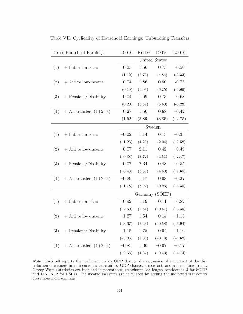
Table VII: Cyclicality of Household Earnings: Unbundling Transfers

Gross Household Earnings L9010 Kelley L9050 L5010United States

(1) + Labor transfers 0.23 1.56 0.73 -0.50(1.12) (5.73) (4.84) (-3.33)

(2) + Aid to low-income 0.04 1.86 0.80 -0.75(0.19) (6.09) (6.25) (-3.66)

(3) + Pensions/Disability 0.04 1.69 0.73 -0.68(0.20) (5.52) (5.60) (-3.28)

(4) + All transfers (1+2+3) 0.27 1.50 0.68 –0.42(1.52) (3.86) (3.85) (–2.75)

Sweden(1) + Labor transfers –0.22 1.14 0.13 –0.35

(–1.23) (4.23) (2.04) (–2.58)

(2) + Aid to low-income –0.07 2.11 0.42 –0.49(–0.38) (3.72) (4.51) (–2.47)

(3) + Pensions/Disability –0.07 2.34 0.48 –0.55(–0.43) (3.55) (4.50) (–2.68)

(4) + All transfers (1+2+3) –0.29 1.17 0.08 –0.37(–1.78) (3.92) (0.96) (–3.30)

Germany (SOEP)(1) + Labor transfers –0.92 1.19 –0.11 –0.82

(–2.60) (2.64) (–0.57) (–3.35)

(2) + Aid to low-income –1.27 1.54 –0.14 –1.13(–3.67) (2.23) (–0.58) (–3.94)

(3) + Pensions/Disability –1.15 1.75 –0.04 –1.10(–3.36) (3.06) (–0.18) (–4.62)

(4) + All transfers (1+2+3) –0.85 1.30 –0.07 –0.77(–2.68) (4.37) (–0.43) (–4.14)

Note: Each cell reports the coefficient on log GDP change of a regression of a moment of the dis-tribution of changes in an income measure on log GDP change, a constant, and a linear time trend.Newey-West t-statistics are included in parentheses (maximum lag length considered: 3 for SOEPand LINDA, 2 for PSID). The income measures are calculated by adding the indicated transfer togross household earnings.

39

To sum up, the government plays an important role in smoothing the businesscycle fluctuations in skewness, which is a crucial aspect of idiosyncratic income risk.The key contributors to this smoothing are unemployment benefit type policies aswell as income taxation. One point that we have not discussed so far but is in factcrucial for an overall assessment is the cost at which this smoothing comes. To see anextreme example, a 100% income tax coupled with a lump sum transfer will completelyeliminate all idiosyncratic income risk but is clearly not a sensible or practical policy.But it illustrates the point that the potential benefits from dampening of skewnessfluctuations delivered by income taxation must be weighed against the myriad othereffects of, including the distortions created by, an income tax system. Such an analysisrequires a full fledged dynamic model, which is beyond the scope of this paper.

7 ConclusionThis paper has characterized how higher-order income risk varies over the business

cycle, as well as the extent to which such risk can be smoothed within households orwith government social insurance policies. We have studied panel data on individualsand households from the United States, Germany, and Sweden, covering more thanthree decades for each country. This allowed us to take a broad perspective whenapproaching the two sets of questions raised in the introduction. One, what is theprecise nature of idiosyncratic income risk, and how does it change in recessions? Andtwo, how successful are various ways by which individual income fluctuations are mit-igated in an economy, which prevents these fluctuations from affecting an individual’sconsumption?

We documented first that the underlying variation in higher-order risk is similaracross these countries that differ in many details of their labor markets. In particular,in all three countries, the variance of earnings changes is almost entirely constant overthe business cycle, whereas the skewness becomes much more negative in recessions.We further showed that these general patterns hold true for different groups definedby education, gender, public- versus private-sector jobs, and occupation. Also, wedocumented that the relationship between skewness and average earnings changes holdsfor longer-horizon income changes as well, and thus affecting persistent income changes.

Second, the skewness cyclicality of individual earnings is a robust feature also forfull-time workers who are continuously employed at the same establishment over thebusiness cycle in both Germany and Sweden. An increased left-skewness in aggregate

40

contractions is thus not just driven by a higher occurrence of unemployment periods,but also by income adjustments on-the-job. We complement this analysis by bringingadditional evidence from France, where we observe employer-reported hours worked.The cyclicality of skewness is driven by both hours and wage adjustments, and againthe sample of full-time workers displays strong skewness cyclicality, which is driven byadjustments of hourly wages. For those workers who are not continuously full-timeemployed, the extensive margin of employment adjustment is important to explain theincreased downside risk in contractions.

Third, within-household smoothing appears to be not effective at mitigating individual-level business cycle fluctuations in skewness. It is worth emphasizing that this doesnot contradict the existence of family insurance in general. Instead, it points towardsfamily insurance reaching its limits in particularly hard times. It is consistent with alower ability of each spouse to respond to the other’s income change in recessions. Also,to the extent that spouses work in, e.g., the same regional labor market, or industrythey can be expected to be exposed to similar semi-aggregate shocks. The detailedevaluation of this channel is on our agenda and left for future research.

Fourth, government-provided insurance—unemployment insurance, aid to low-incomehouseholds, social security benefits, among other transfers and taxes—plays an im-portant role in reducing the cyclicality of downside risk in all three countries. Aninteresting assessment that is beyond the scope of this paper would be to quantify therelative roles of automatic stabilizers, active expansions of the social safety net, andtax progressivity (which could be an important driver of changes in the upper tail ofincome changes) through the lens of a structural model.

41

ReferencesAngelopoulos, K., Lazarakis, S. and Malley, J. (2019). Cyclical income risk

in Great Britain. Working paper no. 7594, CESifo.

Bayer, C. and Juessen, F. (2012). The life-cycle and the business-cycle of wage risk- cross-country comparisons. Economics Letters, 117 (3), 831 – 833.

Blass-Hoffman, E. and Malacrino, D. (2016). Employment Time and the Cycli-cality of Earnings Growth. Tech. rep., Department of Economics, Stanford Univer-sity.

Bound, J., Brown, C. and Mathiowetz, N. (2001). Measurement error in surveydata. In J. Heckman and E. Leamer (eds.), Handbook of Econometrics, 59, Elsevier,pp. 3705–3843.

Busch, C. and Ludwig, A. (2020). Higher-Order Income Risk over the BusinessCycle. Cepr dp 14538.

Card, D., Heining, J. and Kline, P. (2013). Workplace Heterogeneity and the Riseof West German Wage Inequality. The Quarterly Journal of Economics, 128 (3),967–1015.

Constantinides, G. M. and Ghosh, A. (2014). Asset Pricing with CountercyclicalHousehold Consumption Risk. Working paper, University of Chicago.

Daly, M., Hryshko, D. and Manovskii, I. (2014). Reconciling estimates of earn-ings processes in growth rates and levels, manuscript.

Decker, R., Haltiwanger, J., Jarmin, R. and Miranda, J. (2015). Where hasall the skewness gone? The decline in highgrowth (young) firms in the US. WorkingPaper 21776, National Bureau of Economic Research.

Dustmann, C., Ludsteck, J. and Schönberg, U. (2009). Revisiting the germanwage structure. Quarterly Journal of Economics, 124 (2), 843–881.

Ferreira, T. (2018). Stock market cross-sectional skewness and business cycle fluc-tuations.

42

Fitzenberger, B., Osikominu, A. and Völter, R. (2006). Imputation rulesto improve the education variable in the IAB employment subsample. SchmollersJahrbuch. Zeitschrift für Wirtschafts- und Sozialwissenschaften, Jg. 126.

Fuchs-Schündeln, N., Krueger, D. and Sommer, M. (2010). Inequality trendsfor germany in the last two decades: A tale of two countries. Review of EconomicDynamics, 13 (1), 103–132.

Golosov, M., Troshkin, M. and Tsyvinski, A. (2016). Redistribution and socialinsurance. American Economic Review, 106 (2), 359–386.

Guvenen, F., Ozkan, S. and Song, J. (2014). The Nature of Countercyclical In-come Risk. Journal of Political Economy, 122 (3), 621–660.

Harmenberg, K. and Sievertsen, H. H. (2018). The Labor-Market Origins ofCyclical Income Risk. Working paper, Institute for International Economic Studies.

Huggett, M. and Kaplan, G. (2016). How large is the stock component of humancapital? Review of Economic Dynamics, 22, 21–51.

Ilut, C., Kehrig, M. and Schneider, M. (2018). Slow to hire, quick to fire: Em-ployment dynamics with asymmetric responses to news. Journal of Political Econ-omy, 126 (5), 2011–2071.

Kaplan, G., Moll, B. and Violante, G. L. (2016). Monetary Policy Accordingto HANK. Working paper, Princeton University.

Kehrig, M. (2011). The Cyclicality of Productivity Dispersion. Working Paper 11-15,Center for Economic Studies, U.S. Census Bureau.

Kim, T.-H. and White, H. (2004). On more robust estimation of skewness andkurtosis. Finance Research Letters, 1 (1), 56–73.

Kirby, C. (1997). Measuring the predictable variation in stock and bond returns.Review of Financial Studies, 10 (3), 579–630.

Kurman, A. and McEntarfer, E. (2017). Downward Wage Rigidity in the UnitedStates: New Evidence from Administrative Data. Working paper.

Kurmann, A. and McEntarfer, E. (2019). Downward Nominal Wage Rigidity inthe United States: New Evidence from Worker-Firm Linked Data. Working Papers19-07, Center for Economic Studies, U.S. Census Bureau.

43

Mankiw, N. G. (1986). The equity premium and the concentration of aggregateshocks. Journal of Financial Economics, 17 (1), 211–219.

OECD (2016). Economic policy reforms 2016: Going for growth interim report. OECDPublishing.

Oh, S. and Wachter, J. A. (2018). Cross-sectional Skewness. Working paper, Whar-ton School at University of Pennsylvania.

Pora, P. and Wilner, L. (2017). The individual dynamics of wage income in franceduring the crisis. Economie et Statistique / Economics and Statistics, (494-496),179–199.

Pruitt, S. and Turner, N. (2018). The Nature of Household Labor Income Risk.Working paper.

Richardson, M. and Stock, J. H. (1989). Drawing inferences from statistics basedon multiyear asset returns. Journal of Financial Economics, 25 (2), 323–348.

Salgado, S., Guvenen, F. and Bloom, N. (2019). Skewed Business Cycles. Work-ing Paper 26565, National Bureau of Economic Research.

Schmidt, L. D. W. (2016). Climbing and Falling Off the Ladder: Asset PricingImplications of Labor Market Event Risk. Working paper, University of Chicago.

Shin, D. and Solon, G. (2011). Trends in men’s earnings volatility: What doesthe panel study of income dynamics show?,. Journal of Public Economics, 95 (7-8),973–982.

Skedinger, P. (2007). The Design and Effects of Collectively Agreed Minimum Wages:Evidence from Sweden. Working Paper Series 700, Research Institute of IndustrialEconomics.

Storesletten, K., Telmer, C. I. and Yaron, A. (2004). Cyclical dynamics inidiosyncratic labor market risk. Journal of Political Economy, 112 (3), 695–717.

vom Berge, P., Burghardt, A. and Trenkle, S. (2013). Sample-of-Integrated-Labour-Market-Biographies Regional-File 1975-2010 (SIAB-R 7510). Tech. rep., Re-search Data Centre (FDZ) of the German Federal Employment Agency (BA) at theInstitute for Employment Research (IAB).

44

Appendices

A Data AppendixThis appendix briefly describes the variables used for each of the datasets and lists thenumbers of observations after the sample selection steps.

A.1 PSID

Variables

Demographic and SocioeconomicHead and Relationship to Head. We identify current heads and spouses as thoseindividuals within the family unit with Sequence Number equal to 1 and 2, respec-tively. In the PSID, the man is labelled as the household head and the woman as hisspouse. Only when the household is headed by a woman alone is she considered thehead. If the family is a split-off family from a sampled family, then a new head isselected.

Age. The age variable recorded in the PSID survey does not necessarily increase by1 from one year to the next. This may be perfectly correct, since the survey datechanges every year. For example, an individual can report being 20 years old in 1990,20 in 1991, and 22 in 1992. We thus create a consistent age variable by taking the agereported in the first year that the individual appears in the survey and add 1 to thisvariable in each subsequent year.

Education Level. In the PSID, the education variable is not reported every year andit is sometimes inconsistent. To deal with this problem, we use the highest educationlevel that an individual ever reports as the education variable for each year. Since oursample contains only individuals that are at least 25 years old, this procedure does notaffect our education variable in a major way.

IncomeIndividual Male Wages and Salaries. This is the variable used for individualincome in the benchmark case. It is the answer to the question: How much did(Head) earn altogether from wages or salaries in year t-1, that is, before anythingwas deducted for taxes or other things? This is the most consistent earnings variable

1

over time reported in the PSID, as it has not suffered any redefinitions or change insubcomponents.31

Individual Male Labor Earnings. Annual Total Labor Income includes all in-come from wages and salaries, commissions, bonuses, overtime and the labor part ofself-employment (farm and business income). Self-employment in PSID is split intoasset and labor parts using a 50-50 rule in most cases. Because this last component hasbeen inconsistent over time,32 we subtract the labor part of business and farm incomebefore 1993.

Individual Female Labor Earnings. There is no corresponding Wages and Salariesvariable for spouses. We use Wife Total Labor Income and follow a similar procedureas in the case of heads.

Annual Hours. For heads and wives, annual hours is defined as the sum of annualhours worked on main job, extra jobs, and overtime. It is computed using usual hoursof work per week times the number of actual weeks worked in the last year.

Pre-Government Household Labor Earnings. Head and wife labor earnings.

Post-Government Household Labor Earnings. Pre-government household earn-ings minus taxes plus public transfers, as defined below.

Taxes. The PSID reports own estimates for total taxes until 1991. For the remainingyears, we estimate taxes using TAXSIM.

Public Transfers. Transfers are considered at the family unit level whenever possi-ble. We group social and welfare programs into three broad categories. Due to changesin the PSID design, the specific definition of each program is different every year. Wegive an overview below and leave the specific replication details for the online DataAppendix.

TransfersSee Table A.1 below for a description of the three groups of programs considered, aswell as their subcomponents. In the PSID, obtaining an annual amount of each type

31See Shin and Solon (2011) for a comparison of PSID male earnings variables in inequality analyses.32In particular, total labor earnings included the labor parts of farm and business income up to

the 1993 survey but not in subsequent waves.

2

of benefits is almost wave-specific. Every few survey years, the level of aggregationwithin the family unit and across welfare programs is different for at least one of ourgroups. To impose some common structure, we establish the following rules.

For survey years 1970-199333 and 2005-2011, the total annual amount of each pro-gram is reported for the head, spouse, and others in the family unit. Occasionally,the amount appears combined for several or all members.34 Because in those cases itis impossible to identify separate recipiency of each member, we consider the benefitamount of the whole family. That is, we add up all available information for all familymembers, whether combined or separately reported.

In survey years 1994-2003, most benefits (except Food Stamps and OASDI) arereported separately for the head and the spouse only. The way amounts are reportedchanges as well. First, the reported amount ($X) received is asked. Second, thefrequency of that amount ($X per year, per month, per week, etc.) is specified. Weconvert all amounts to a common frequency by constructing a monthly amount $x

using these time values. Finally, the head and spouse are asked during which monthsthe benefit was received. The final annual recipiency of transfers is then obtained bymultiplying $x by the number of months this benefit was received. For Food Stampsand OASDI, we follow the rules described for the other waves.

Detailed Sample Selection

We start with an initial sample of 584,392 SRC individuals interviewed between 1976and 2011. We then impose the next criteria every year. The number of individuals keptat each stage in the sample selection is listed in Table A.2. Previous to this selectionprocess, we have cleaned the raw data and corrected duplicates and inconsistencies(for example, zero working hours with positive labor income). We also require thatthe individuals have non top-coded observations in income.

1. The individual must be from the original main PSID sample (not from the Surveyof Economic Opportunities or Latino subsamples).

2. In the benchmark individual sample, we select male heads of family. In the ref-erence household sample, we require at least two adult members in the unit and

33Our main sample refers to survey years 1977-2011, but complementary results are provided forthe annual subsample of the PSID, that is, for 1970-1997. We drop the first two waves in all cases,since benefits such as OASDI, UI, and WC are only reported for the family head and benefits suchas SSI are not reported at all.

34This is always the case for Food Stamps.

3

Table A.1: Components of Social Policy

LINDA SOEP PSID1. Labor market transfers: Unemployment

benefits;Labor market programs

Unemployment benefits Unemploymentbenefits;Workers’ compensation

2. Aid to low-income families: Family support;Housing support;Cash transfers from thepublic;(no private transfers)

Subsistence allowance;Unemploymentassistance(up to 2004);Unemployment benefitsII (since 2005)

Supplemental SecurityIncome;Aid to Families withDependent Children(AFDC);Food Stamps;Other Welfare

3. Social security and pensions: (Old Age) Pensions Combined old-age,disability, civil service,and company pensions

Combined (Old Age)Social Security andDisability (OASI)

Note: The table lists the measures used in the three datasets to construct subcompo-nents of transfers.

that individuals had no significant changes in family composition. More specif-ically, we require that they responded either “no change” or “change in familymembers other than the head or wife” to the question about family compositionchanges.

3. The household must not have missing variables for the head or wife labor income,or for education of the head. The individuals must not have missing income oreducation themselves.

4. The individual must not have income observations that are outliers. An outlieris defined as being in the top 1% of the corresponding year.

5. We require the income variable of analysis to be positive.

6. Household heads must be between 25 and 65 years old.

A.2 LINDAVariables

Demographic and SocioeconomicHead and Relationship to Head. LINDA is compiled from the Income Registerbased on filed tax reports and other registers. Statistics Sweden samples individualsand then adds information for all family members, where family is defined for tax

4

Table A.2: Number of Observations Kept in Each Step: PSID

Male Heads Households All FemalesSRC 586,187 586,187 586,187Family Composition 90,106 75,202 110,711Non-Missing y or College 83,039 69,443 97,990Positive Income 63,875 58,551 54,214Outliers 63,065 57,262 53,257Age Selection 54,593 50,102 45,330Final #Obs for transitory changes 42,623 38,171 33,687Final #Obs for persistent changes 34,985 30,985 27,269

Note: Table lists number of person-year, or household-year, observations in the three panels for thesample from PSID.

purposes. This implies that there is no information about “head of households.” Wetherefore define the head of a household as the sampled male.

Age. As defined by Statistics Sweden.

Education Level. LINDA contains information about education from 1991 and on-ward. An individual is assigned “college” education if he/she has at least three yearsof university education.

Private/Public employment An individual is defined as as working in the publicsector, if he/she works in public administration, health care or education. LINDAcontains consistent comparable information for the years 1991 and onward. For theyears 1991-1992, we use SNI90 codes 72000-72003, 90000-93999, and >=96000 to definepublic sector employment. For 1993-2006, we use SNI92 codes 64110-64202, 73000-74110, 75000-92000, 92500-92530, and >=96000. For 2007-2010, we use SNI2007 codes64110-64202, 73000-74110, 75000-92000, 92500-92530, and >=96000.

IncomeFor the years 1985-2010, we use the measures suggested by Statistics Sweden to becomparable between years in LINDA. We construct comparable measures for the years1979-1984.

Individual Labor Earnings. Labor earnings consist of wages and salaries, the partof business income reported as labor income, and taxable compensation for sick leaveand parental leave.

Pre-Government Household Labor Earnings. Defined as the sum of individuallabor income within the family.

5

Post-Government Household Labor Earnings. Post-government earnings is cal-culated as pre-government earnings minus taxes plus public transfers.

Taxes. LINDA provides observations of total taxes paid by the individual. Sincetaxes paid on capital income constitute a small part of total tax payments, and sincewe cannot separate taxes on capital income from those on labor income, we assumethat all taxes are labor income taxes.

Public Transfers. LINDA provides observations of total public transfers at the in-dividual level (Statistics Sweden has individualized transfers given to families) and atthe household level. We also consider three subcategories of transfer as listed below.

TransfersTransfers in subcategories 1 and 3 are individual-level transfers. Transfers in subcat-egory 2 are family level transfers but have been individualized by Statistics Sweden.For each subcategory, we take all transfers received by all members of the households.

• HH-level transfers subcategory 1 (labor market transfers): sum of unemploymentbenefits received by all members of household.

• HH-level transfers subcategory 2 (family aid): sum of transfers to support familiesreceived by all members of household.

• HH-level transfers subcategory 3 (pensions): sum of old-age pensions received byall members of household.

Detailed Sample Selection

To be included in the individual sample, the individual has to be sampled and between25 and 60 years old. A family is included in the household sample if the sampledindividual is a man between 25 and 60 years old and there are at least two membersages 25-60 in the family.

A.3 LISAThe LISA database covers all individuals between 16 and 64 years of age for the

period 1990-95 and all individuals above age 16 thereafter. Like in LINDA, all incomedata is based on tax records. Using the same definitions for all variables and the samesample selection procedure as in LINDA results in a sample with around 1.6 million

6

one-year income changes per year. It contains annual information on employers of indi-viduals, as well as on the establishment. We use this additional information in order toidentify workers that stay at the same main establishment for a given t to t+1 change.We restrict this sample of stayers to individuals whose main establishment in both tand t+1 is the same, and who in addition received income from this establishment inboth t-1 and t+2.

A.4 SIABWe use the scientific use file SIAB-R7510 provided by the Institute for EmploymentResearch (IAB). The SIAB data from which the scientific use file is constructed are a2% random sample of all individuals covered by a dataset called IEB. This dataset isfrom four different sources, which can be identified in the data. For construction ofour sample, we use earnings data stemming from BeH (employee history) and transferdata from LeH (benefit recipient history). Records in BeH are based on mandatorysocial security notifications from employers and hence cover individuals working inemployment subject to social security, which excludes civil servants, students, andself-employed individuals. A new spell starts whenever there is a new notification,which happens when a new employment relationship changes, an ongoing contractis changed, or a new calendar year starts. BeH covers all workers subject to socialsecurity contributions, which excludes civil servants, self-employed individuals andstudents. For details on the dataset, see vom Berge et al. (2013).

Variables

Demographic and SocioeconomicHead and Relationship to Head. SIAB does not contain information on house-holds. We use only individual-level data.

Age. Birth year is reported consistently in SIAB data.

Education Level. Each individual spell in SIAB contains information on the high-est degree of formal education as reported by the employer. In order to construct aconsistent measure of education we apply imputation rules proposed by Fitzenbergeret al. (2006).

Private/Public Employment. An individual is defined as working in the pub-lic sector, if he/she works in public administration, health care or education. SIABcontains consistent comparable information for all years of the sample. We use the

7

classification WZ93 as provided in the data, which aggregates 3-digit codes of the orig-inal WZ93 classification into 14 categories. The industry of an employer is registeredonce a year and assigned to the worker spells of that year. This implies that for someindividual spells, there is no information on the industry. For each year, a worker isassigned the industry from the longest spell in that year. We classify as public em-ployment those in sectors 13 (3-digit WZ93 801-804, 851-853: Education, social, andhealth-care facilities) and 14 (751-753, 990: public administration, social security).

IncomeIndividual Labor Earnings. We calculate annual earnings as the sum of totalearnings from all valid spells for each individual. As marginal employment spells werenot reported before 1999, we drop marginal employment in the years where they arereported in order to obtain a time consistent measure. For the same reason, we dropspells with a reported average daily wage rate below the highest marginal employmentthreshold in the sample period, which is 14.15 euros (in 2003 euros). The available datahave two drawbacks: the structural break of the wage measure in 1984 and top-coding.

Structural Break in Wage Measure. Since 1984 the reported average daily wagerate from an employment spell includes one-time payments. We correct for this struc-tural break following a procedure based on Dustmann et al. (2009): we rank individualsfrom 1976 to 1983 into 50 quintiles of the annual full-time wage distributions. Then wefit locally weighted regressions of the wage growth rate from 1982 to 1983 on the quin-tiles in 1983 and the same for 1983 to 1984. We then define as the correction factor thedifference between the quintile-specific smoothed value of wage growth between 1984and 1983. The underlying assumption is that wage growth should be higher from 1983to 1984 because the wage measure includes one-time payments. In order to controlfor overall wage growth differences, we subtract the average of the correction factor ofthe second to 20th quintiles. The resulting percentile-specific correction factor is thenapplied to wages in 1976-1983.

Imputation of Top-Coded Wages. Before aggregating earnings from all spells, wecorrect full-time wage spells for the top-coding. We therefore follow Daly et al. (2014)and fit a Pareto tail to the cross-sectional wage distribution. The Pareto distribution isestimated separately for each year by age group and sex. We define seven age groups:25-29, 30-34,...,55-60. As a starting point for the Pareto distribution, we choose the60th percentile of the subgroup-specific distribution. As in Daly et al. (2014), wedraw one random number by individual, which we then apply to the annual specific

8

distributions when assigning a wage to the top-coded workers. We apply the imputationmethod to the annual distribution of average full-time wages, and hence an individualcan be below the cutoff limit if, for example, from two full-time spells in a year onlyone is top-coded. We therefore define as the top-coding limit the annual specific limitminus 3 DM (1995 DM) as in Dustmann et al. (2009).

TransfersIn SIAB we observe consistently over time unemployment benefits at the individuallevel.

Detailed Sample Selection

To be included in the sample, the individual has to be between 25 and 60 years oldand earn a gross income above 520*0.5*minimum wage. We drop all workers that haveat least one spell reported in East Germany.

A.5 SOEPVariables

Demographic and SocioeconomicHead and Relationship to Head. For each individual in the sample, SOEP reportsthe relationship to the head of household in any given wave. Whenever there is a non-couple household, (that is no spouse is reported), the reported head is classified ashead. Whenever we observe a couple household and the reported head is a male, wekeep this; when the reported head is a female and the reported spouse is a male, wereclassify the male to be head and the female to be spouse.

Age. The age is measured by subtracting the year of birth from the current year.

Education Level. The education variable used categorizes the obtained maximumeducation level by ISCED 1997. An individual with category 6 is assigned “college”education; an individual with categories 1-5 is assigned “non-college.” Category 6includes a degree obtained from a university, from technical college, from a universityabroad, and a PhD. An individual still in school (category 0) is assigned a missingvalue. For a small number of individuals, the described procedure yields inconsistenciesin the sense that for some year t, the assignment is “college” and some later year t+sthe assignment is “non-college”; in these cases, we assign “college” to the later year.

9

Income and HoursIndividual Labor Income. Labor earnings are calculated from individual laborincome components and include income from first job, secondary job, 13th and 14thsalary, Christmas bonus, holiday bonus, and profit sharing. For consistency with thePSID measure, we assign 50% of income from self-employment to labor income.

Household-Level Labor Income. Defined as the sum of individual labor incomeof head and spouse.

Annual Hours. SOEP measures the average actual weekly hours worked and thenumbers of months an individual worked. From these measures SOEP, provides aconstructed measure of annual hours worked of an individual.

Pre-Government Household Labor Earnings. Head and spouse labor earnings.

Post-Government Household Labor Earnings. Pre-government household earn-ings minus taxes plus public transfers, as defined below.

Taxes. SOEP provides estimates of total taxes at the household level.

Public Transfers. Transfers are considered at the family unit level and at the in-dividual level. We group social and welfare programs into three broad categories aslisted below.

TransfersTransfers are partly observed at the individual level and partly at the household level.For each subcategory, we take all transfers received by all members of the households.

• HH-level transfers: we use transfers received by all individual household mem-bers in order to calculate measures that are consistent over time. For eachindividual, total transfers are the sum of the following components: old-agepensions, widow’s pensions, maternity benefit, student grants, unemploymentbenefits, subsistence allowance, unemployment assistance (up to 2004); at thehh-level we measure received child allowances and the total unemployment ben-efits II received by all household members (since 2005 replacing unemploymentassistance).

10

• HH-level transfers subcategory 1 (labor market transfers): sum of unemploymentbenefits received by all members of household.

• HH-level transfers subcategory 2 (family aid): sum of subsistence allowance ofall members, + sum of unemployment assistance received by all members (up to2004), + hh-level measure of unemployment benefits II (since 2005).

• HH-level transfers subcategory 3 (pensions): sum of old-age pensions received byall members of household.

Sample Selection

In order to be in the initial sample for a year, the individual or household head mustbe between ages 25 and 60 and live in West Germany. In order to have a consistentsample, we drop the immigrant subsample and the high-income subsample. This givesinitial sample sizes of 87,582 individual-year observations for the male sample, 76,249individual-year observations for the female sample, and 76,051 household-year observa-tions for the household sample (see Table A.3). The sample selection then follows thesteps listed below for each sample. All cross-sectional statistics are calculated usingappropriate cross-sectional individual or household weights, respectively.

1. drop if no info on education or if no degree obtained yet

2. drop if currently working in military

3. drop if no info on income

4. drop if no info on hours worked

5. keep if income > 0 and hours ≥ 520

6. drop if in highest percentile (sample outliers)

7. drop if below 520*0.5*minimum wage, where minimum wage is set to be 6€ inyear 2000 euros

8. for transitory change measure: keep if in sample in t and t-1

9. for permanent change measure: keep if in sample in t and t-5

11

Table A.3: Number of Observations Kept in Each Step: SOEP

selection step Male Heads Households All Femalesinitial 87,582 95,982 95,716drop if no coll. info 86,737 95,008 94,456drop if in military 86,712 94,990 94,454drop if no obs on ymin 86,009 94,990 93,960drop if no obs on hours 86,009 94,990 93,960keep if >=520 hrs and ymin>0 77,501 87,332 57,979drop top 1% of ymin per year 76,641 86,379 57,475drop if ymin<.5*520*min wage 76,460 85,429 56,803Final #Obs for transitory changes 64,824 71,287 44,805Final #Obs for persistent changes 38,555 41,048 24,968

Note: Table lists number of person-year, or household-year, observations in the three panels for thesample from SOEP.

A.6 DADSThe DADS (“Declaration Annuelle des Donnees Sociales”) panel is extracted from

exhaustive administrative records of annual employer-employee information with com-pulsory completion by all firms and establishments within firms. These administrativerecords are used for taxation and social security purposes. All private sector firms,regardless of the number of employees, are included. Regarding the public sector, itincludes dependent workers from semi-public firms. To constitute the panel, a 4% sam-ple of workers was extracted from the records since 1976 and until 2001. These consistof all workers born in October of an even calendar year. Since 2002, workers bornin October of all years have been included. This results in samples of approximately8%. We use data on earnings, number of days paid, start and end date of the spell,and, importantly, number of hours worked, which is recorded since 1993. Due to dataprocessing changes between 1993 and 1994, those years are dropped in the analysis,and thus we end up with usable data from 1995–2015. Given the similar nature of thedataset, we follow the same basic steps of sample selection as for the SIAB.

12

Figure B.1: L9050 and L5010 against the Quartiles of Log GDP Change: Males

(a) Upper Tail (L9050) (b) Lower Tail (L5010)

Note: For different samples, each bar shows the average moment across years and countries by quartilesof log GDP change. Both log GDP changes and moments are standardized by country.

B Cyclicality of Individual Earnings by Groups

B.1 Education and Sector of Employment

Figure B.1 complements Figure 6 in the text and reports L9050 and L5010 formales in the same format. The next figure (B.2) reports the counterparts of these twofigures for females.

Furthermore, we show results of the individual level earnings regressions discussed inSection 4 by subgroups. For each group and country, we estimated our baseline regres-sion (equation 3). The estimated sensitivity coefficients are displayed in Figure B.3,followed by Tables B.1 to B.5 showing the specific estimates, as well as the correspond-ing t-statistics. Each panel in the figure shows, starting from the left, the regressioncoefficients along with 95% confidence intervals for males (solid) in Sweden (red, trian-gles), Germany (green, squares), and the US (blue, bullets), followed by the equivalentregression coefficients for females (dotted). Within each country-gender grouping, thecoefficients are (ordered from the left) those from the full sample, college graduates,non-college graduates, private employment, and public employment, respectively.

Figure B.3 confirms the picture that emerged in Figures 6 and B.2: higher-orderearnings risk is similar across groups. However, we see some noteworthy differences.

13

Figure B.2: Higher-Order Moments by Quartiles of Log GDP Change: Females

(a) Dispersion (L9010) (b) Kelley skewness

(c) Upper Tail (L9050) (d) Lower Tail (L5010)

Note: For different samples, each bar shows the average moment across years and countries by quartilesof log GDP change. Both log GDP changes and moments are standardized by country.

The magnitude of cyclicality is stronger for non-college graduates as compared tocollege graduates. The difference is particularly large for males in the US and Sweden,where the regression coefficient for Kelley skewness is about two to three times largerfor non-college graduates (insignificant 0.97 vs. 2.37 for the US and 1.80 vs. 4.03 forSweden). Moreover, the magnitude of cyclicality for public sector workers is weaker inall countries—and insignificant in the cases of Germany and the US.

In Sweden, the procyclicality of Kelley’s measure of earnings is lower for the publicsector (2.10 for males and 1.10 for females) compared with the private sector (3.83 for

14

males and 1.99 for females). For males, this is due to differences in the top tail; itcompresses strongly for private sector employees, whereas it is acyclical in the publicsector. The L5010 gap, on the other hand, fluctuates by comparable magnitudes forboth groups. For women, the reduced cyclicality is due to both tails fluctuating slightlyless.

Overall, it is somewhat surprising that for workers in the public sector in a coun-try like Sweden with a reputation for high levels of public insurance, there is robustevidence of higher downside risk in recessions—compression of the top and expan-sion of the bottom of the distribution of income changes—even if the magnitudes aresomewhat smaller than in the private sector.35 This finding further strengthens theconclusion in Section 4 that increasing downside (individual) earnings risk appears tobe a robust feature of business cycles in developed countries.

35One explanation (suggested by a referee) could be in employment protection that creates con-centration of earnings changes. If most workers’ earnings cannot fall by statute or contract, thenthe measured declines of earnings are likely to be concentrated among the set of people who work atfirms that are sufficiently hard hit, which would then generate an expansion of the left tail of earningschanges.

15

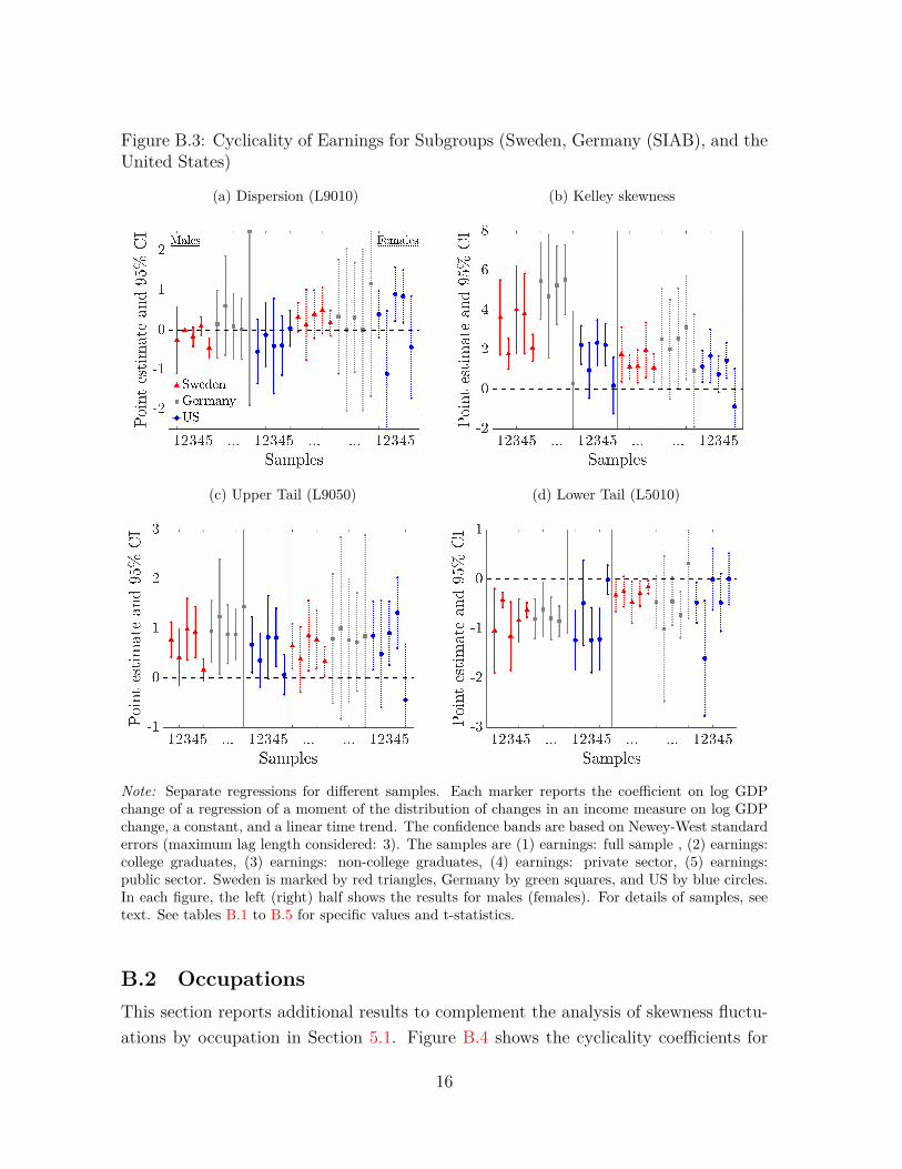
Figure B.3: Cyclicality of Earnings for Subgroups (Sweden, Germany (SIAB), and theUnited States)

(a) Dispersion (L9010) (b) Kelley skewness

(c) Upper Tail (L9050) (d) Lower Tail (L5010)

Note: Separate regressions for different samples. Each marker reports the coefficient on log GDPchange of a regression of a moment of the distribution of changes in an income measure on log GDPchange, a constant, and a linear time trend. The confidence bands are based on Newey-West standarderrors (maximum lag length considered: 3). The samples are (1) earnings: full sample , (2) earnings:college graduates, (3) earnings: non-college graduates, (4) earnings: private sector, (5) earnings:public sector. Sweden is marked by red triangles, Germany by green squares, and US by blue circles.In each figure, the left (right) half shows the results for males (females). For details of samples, seetext. See tables B.1 to B.5 for specific values and t-statistics.

B.2 OccupationsThis section reports additional results to complement the analysis of skewness fluctu-ations by occupation in Section 5.1. Figure B.4 shows the cyclicality coefficients for

16

Table B.1: Cyclicality of Male Earnings, by Education Groups

L9010 Kelley L9050 L5010United States

College Graduates –0.12 0.97 0.36 –0.48(–0.31) (1.42) (1.39) (–1.15)

Non-College –0.40 2.37 0.83 –1.23(–0.69) (4.29) (2.04) (–3.88)

SwedenCollege Graduates –0.00 1.80 0.42 –0.42

(–0.01) (4.93) (1.58) (–5.72)Non-College –0.17 4.03 0.99 –1.15

(–1.52) (3.86) (3.39) (–3.53)Germany (SIAB)

College Graduates 0.62 4.70 1.24 –0.61(1.01) (3.10) (2.17) (–2.29)

Non-College 0.10 5.26 0.89 –0.79(0.25) (5.41) (3.07) (–3.78)

Note: Each cell reports the coefficient on log GDP change of a regression of a moment of the dis-tribution of changes in an income measure on log GDP change, a constant, and a linear time trend.Newey-West t-statistics are included in parentheses (maximum lag length considered: 3 for SIAB andLINDA, 2 for PSID).

L5010 and L9050 to complement the L9010 and Kelley skewness shown in Figure 7.Table B.5 reports the cyclicality regressions for five broader occupational categoriesas instead of the 30 detailed categories in Figure 7). Figures B.5 and B.6 are theanalogues of Figures 7 and B.6 for females.

17

Table B.2: Cyclicality of Female Earnings, by Education Groups

L9010 Kelley L9050 L5010United States

College graduates –1.11 1.70 0.49 –1.60(–1.44) (2.61) (0.94) (–2.84)

Non-college 0.91 0.78 0.91 –0.00(2.77) (1.75) (2.91) (–0.01)

SwedenCollege graduates 0.13 1.15 0.28 –0.25

(0.31) (4.03) (1.22) (–1.74)Non-college 0.50 1.81 0.75 –0.25

(1.96) (3.40) (2.78) (–2.71)Germany (SIAB)

College graduates 0.01 2.03 1.01 –1.00(0.01) (1.65) (1.12) (–1.39)

Non-college 0.32 2.58 0.77 –0.45(0.47) (2.08) (1.27) (–1.88)

Note: Each cell reports the coefficient on log GDP change of a regression of a moment of the dis-tribution of changes in an income measure on log GDP change, a constant, and a linear time trend.Newey-West t-statistics are included in parentheses (maximum lag length considered: 3 for SIAB andLINDA, 2 for PSID).

18

Table B.3: Cyclicality of Individual Earnings, Public vs. Private Sector Employment,Males

L9010 Kelley L9050 L5010United States

Private –0.39 2.26 0.82 –1.21(–1.08) (4.43) (2.88) (–4.03)

Public 0.05 0.20 0.07 –0.01(0.23) (0.29) (0.36) (–0.07)

SwedenPrivate 0.10 3.83 0.93 –0.83

(0.93) (4.02) (3.81) (–4.08)Public –0.45 2.10 0.17 –0.62

(–3.93) (6.55) (1.64) (–9.11)Germany

Private 0.03 5.55 0.88 –0.85(0.08) (6.44) (3.55) (–5.64)

Public 2.50 0.30 1.45 1.06(1.16) (0.17) (1.08) (1.01)

Note: Each cell reports the coefficient on log GDP change of a regression of a momentof the distribution of changes in an income measure on log GDP change, a constant,and a linear time trend. Newey-West t-statistics are included in parentheses (maximumlag length considered: 3 for SIAB and LINDA, 2 for PSID).

19

Table B.4: Cyclicality of Individual Earnings, by Sector of Employment, Females

L9010 Kelley L9050 L5010United States

Private 0.85 1.47 1.32 –0.47(2.64) (3.38) (3.82) (–1.67)

Public –0.43 –0.87 –0.44 0.01(–0.69) (–0.94) (–0.81) (0.04)

SwedenPrivate 0.50 1.99 0.78 –0.29

(1.87) (3.02) (2.81) (–2.43)Public 0.18 1.10 0.34 –0.16

(1.19) (3.29) (2.43) (–2.61)Germany

Private 0.01 3.13 0.73 –0.72(0.01) (2.44) (1.50) (–3.15)

Public 1.17 0.95 0.85 0.32(0.84) (0.68) (0.85) (0.59)

Note: Each cell reports the coefficient on log GDP change of a regression of a momentof the distribution of changes in an income measure on log GDP change, a constant,and a linear time trend. Newey-West t-statistics are included in parentheses (maximumlag length considered: 3 for SIAB and LINDA, 2 for PSID).

20

Figure B.4: Tails of Short-Run Income Growth by Occupation: Males (Germany(SIAB))

(a) Upper Tail (L9050)

(b) Lower Tail (L5010)Note: Separate regressions for each of 30 occupation segments. Each marker reports the coefficient onlog GDP change of a regression of a moment of the distribution of changes in an income measure onlog GDP change, a constant, and a linear time trend. The confidence bands are based on Newey-Weststandard errors (maximum lag length considered: 3)

21

Table B.5: Cyclicality of Earnings by Occupational Area: Germany (SIAB)

L9010 Kelley L9050 L5010Males

Farming and related 4.56 5.64 3.80 0.76(1.23) (1.51) (1.52) (0.45)

Mining, Mineral Extraction 2.62 3.23 1.32 1.30(1.25) (1.39) (2.43) (0.72)

Manufacturing, Fabrication 0.17 11.39 2.00 -1.83(0.20) (5.53) (3.21) (-3.99)

Technical Occupations 0.13 12.36 1.51 -1.38(0.19) (4.04) (2.72) (-3.64)

Service Occupations 0.59 8.89 1.76 -1.17(0.68) (3.92) (2.41) (-3.09)

FemalesFarming and related 2.90 0.96 2.06 0.84

(0.73) (0.31) (0.71) (0.61)Mining, Mineral Extraction -5.59 12.26 1.61 -7.20

(-1.02) (1.54) (0.34) (-2.59)Manufacturing, Fabrication -0.72 10.59 2.48 -3.20

(-0.48) (4.95) (2.00) (-6.01)Technical Occupations -0.75 8.44 1.41 -2.16

(-0.83) (2.70) (1.56) (-2.82)Service Occupations 0.85 4.09 1.45 -0.60

(0.59) (1.63) (1.13) (-1.15)

Note:Each cell reports the coefficient on log GDP change of a regression of a momentof the distribution of changes in an income measure on log GDP change, a constant,and a linear time trend. Newey-West t-statistics are included in parentheses (maximumlag length considered: 3).

22

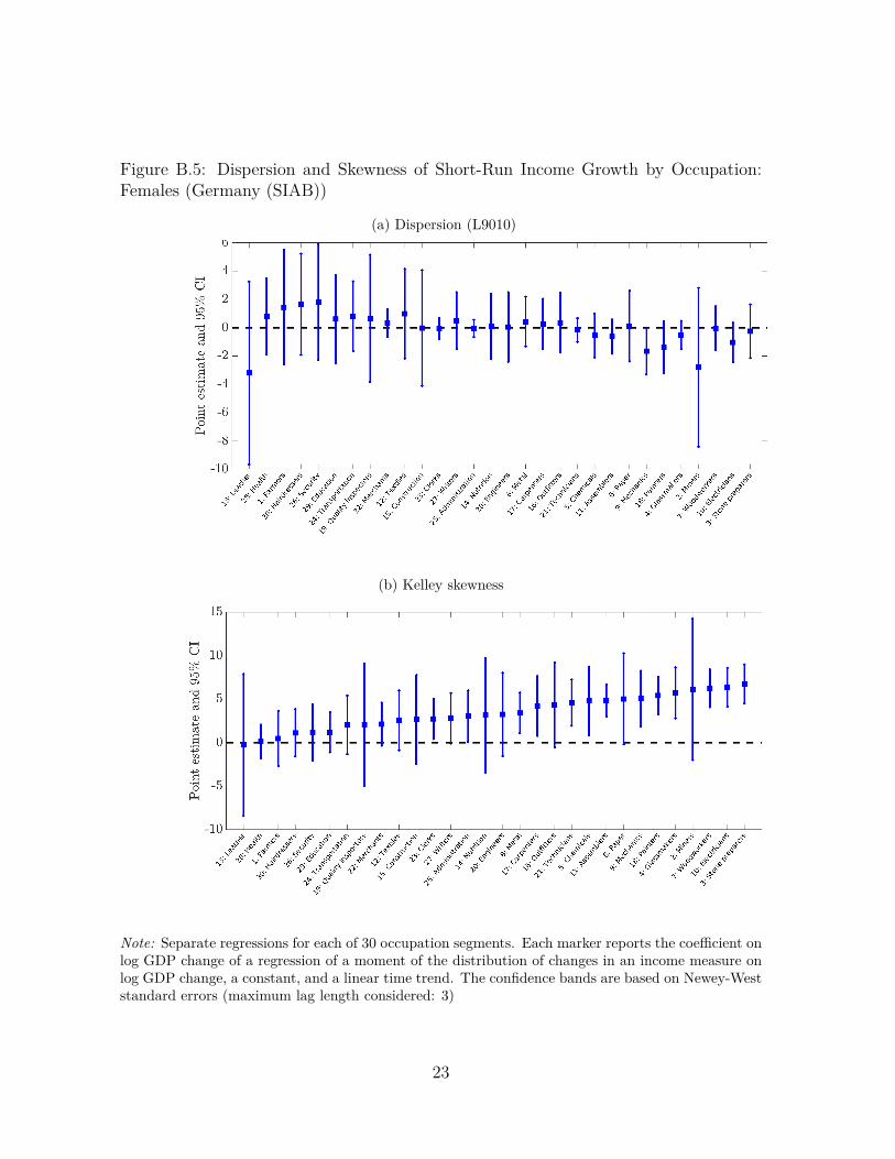
Figure B.5: Dispersion and Skewness of Short-Run Income Growth by Occupation:Females (Germany (SIAB))

(a) Dispersion (L9010)

(b) Kelley skewness

Note: Separate regressions for each of 30 occupation segments. Each marker reports the coefficient onlog GDP change of a regression of a moment of the distribution of changes in an income measure onlog GDP change, a constant, and a linear time trend. The confidence bands are based on Newey-Weststandard errors (maximum lag length considered: 3)

23

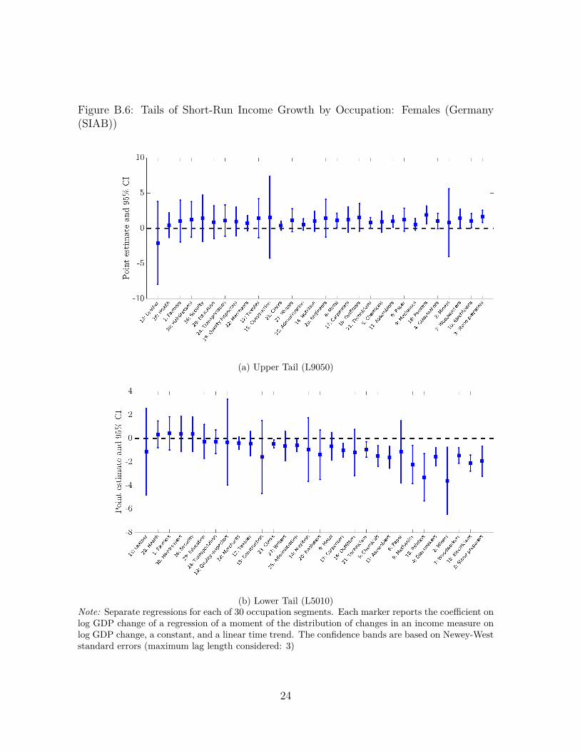
Figure B.6: Tails of Short-Run Income Growth by Occupation: Females (Germany(SIAB))

(a) Upper Tail (L9050)

(b) Lower Tail (L5010)Note: Separate regressions for each of 30 occupation segments. Each marker reports the coefficient onlog GDP change of a regression of a moment of the distribution of changes in an income measure onlog GDP change, a constant, and a linear time trend. The confidence bands are based on Newey-Weststandard errors (maximum lag length considered: 3)

24

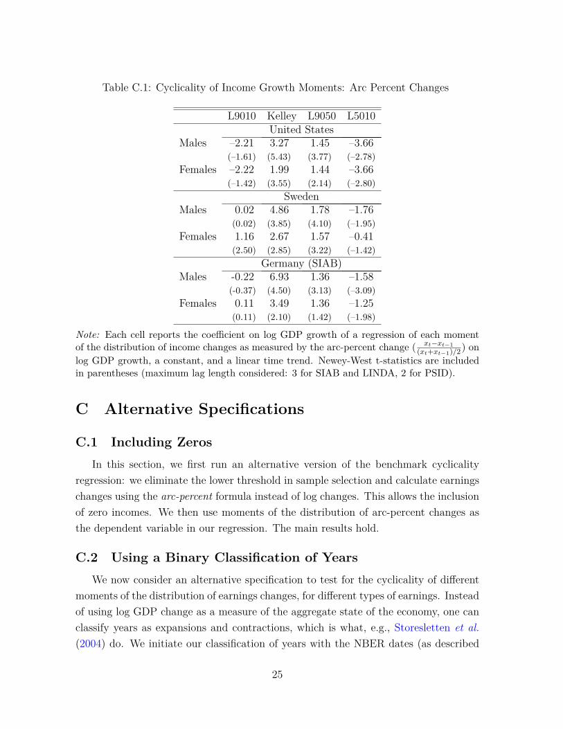
Table C.1: Cyclicality of Income Growth Moments: Arc Percent Changes

L9010 Kelley L9050 L5010United States

Males –2.21 3.27 1.45 –3.66(–1.61) (5.43) (3.77) (–2.78)

Females –2.22 1.99 1.44 –3.66(–1.42) (3.55) (2.14) (–2.80)

SwedenMales 0.02 4.86 1.78 –1.76

(0.02) (3.85) (4.10) (–1.95)Females 1.16 2.67 1.57 –0.41

(2.50) (2.85) (3.22) (–1.42)Germany (SIAB)

Males -0.22 6.93 1.36 –1.58(-0.37) (4.50) (3.13) (–3.09)

Females 0.11 3.49 1.36 –1.25(0.11) (2.10) (1.42) (–1.98)

Note: Each cell reports the coefficient on log GDP growth of a regression of each momentof the distribution of income changes as measured by the arc-percent change ( xt−xt−1

(xt+xt−1)/2) on

log GDP growth, a constant, and a linear time trend. Newey-West t-statistics are includedin parentheses (maximum lag length considered: 3 for SIAB and LINDA, 2 for PSID).

C Alternative Specifications

C.1 Including ZerosIn this section, we first run an alternative version of the benchmark cyclicality

regression: we eliminate the lower threshold in sample selection and calculate earningschanges using the arc-percent formula instead of log changes. This allows the inclusionof zero incomes. We then use moments of the distribution of arc-percent changes asthe dependent variable in our regression. The main results hold.

C.2 Using a Binary Classification of YearsWe now consider an alternative specification to test for the cyclicality of different

moments of the distribution of earnings changes, for different types of earnings. Insteadof using log GDP change as a measure of the aggregate state of the economy, one canclassify years as expansions and contractions, which is what, e.g., Storesletten et al.(2004) do. We initiate our classification of years with the NBER dates (as described

25

in the main text). We extend the measure by considering the average growth of maleearnings (as done in Huggett and Kaplan (2016)).36 Our preferred specification remainsthe continuous measure in the main text, because it is more flexible and simplifies thecross-country comparison. Furthermore, it does not come with the difficulty of exactlytiming recessions at the yearly level

Still, there are advantages of resorting to a binary characterization. To beginwith, it makes our results more easily comparable to previous work Storesletten et al.(2004); Pruitt and Turner (2018); Guvenen et al. (2014). More importantly, it teststhe robustness of our results in the case we thought of cyclicality as a regime switchingrather than a linear relationship between the aggregate state and the distribution ofearnings.37

The following tables show regression results for an alternative specification wherewe regress on a dummy that takes the value 1 in expansions instead of regressing on logGDP growth. The results are virtually unchanged, i.e., they tell exactly the same storyas our benchmark specification: entering an expansion is associated with a significantincrease in skewness and a non-significant change in dispersion. We document the fourmain types of earnings, but there are no significant changes from any of the results inthe main text.We focus on the case of the US since the main issue is comparabilitywith previous work—which is focused on the US—and specification robustness. All inall, we can conclude that, if the cyclical relationship is more a regime-switching modelwith reasonable noise and realistic dynamics, our regression picks up the relationship.

36This results in contraction years 1970, 1974, 1980, 1981, 1982, 1983, 1990, 1991, 2001, 2002,2008, 2009, 2010, and 2012.

37We thank one of the referees for suggesting this extension and the thoughtful interpretation.

26

Table C.2: Cyclicality of Individual Earnings using binary Measure of Business Cycles:United States

L9010 Kelley L9050 L5010Males (GOS) 0.00 0.15 0.07 –0.07

(–0.06) (6.66) (6.14) (–4.06)Males -0.02 0.15 0.05 -0.08

(-0.91) (4.17) (3.54) (-3.13)Females 0.04 0.06 0.06 -0.01

(2.10) (2.07) (2.43) (-0.85)HH Earnings 0.01 0.12 0.06 -0.04

(0.63) (5.10) (7.68) (-2.42)HH Post-Gov 0.03 0.08 0.04 -0.01

(2.05) (4.36) (4.70) (-1.23)

Note: Each cell reports the coefficient on a dummy—1 in expansions and 0 in recessions—of a regres-sion of each moment of the distribution of income changes on such dummy, a constant, and a lineartime trend. Newey-West t-statistics are included in parentheses (maximum lag length considered: 2).Males (GOS) uses the moments of Guvenen et al. (2014).

D Hours versus Wages: FemalesTable D.1 shows the regressions of full time workers and stayers for German andSwedish females. Table D.2 shows the results for females in SIAB who are not in thefull-time sample. The results for females mirror the findings for males in the maintext. The systematic variation of skewness of earnings changes over the business cyclecannot be entirely explained by the extensive margin of employment changes. Instead,also the incomes of workers who are continuously full-time employed over the cycledisplay an increase of left-skewness in aggregate downswings.

E Survey versus Administrative DataAs noted earlier, it is not possible to link individual data from the SIAB dataset

to obtain household-level information. This is why we use survey data (PSID for theUS and SOEP for Germany) to answer questions regarding insurance provided withinhouseholds and by the government. These datasets, however, suffer from having fairlyfew observations, which may imply that higher moments are imprecisely estimated.

Specifically, we have rerun the regression in equation (3) using moments from theSSA data (reported in Guvenen et al. (2014)), and from SOEP data. The resultingcoefficients for US males using SSA data for each of the four moments are –0.07, 2.31,

27

Table D.1: Cyclicality of Individual Earnings vs. Daily Wages; Germany (SIAB) andSweden (LISA): Females

L9010 Kelley L9050 L5010Germany

Earnings (Full population) 0.34 2.55 0.80 –0.46(0.48) (2.05) (1.25) (–1.80)

Full-Time Daily Wages 0.03 2.12 0.17 –0.14(0.18) (5.11) (2.61) (–1.58)

Full-Time Daily Wages 0.02 2.28 0.16 –0.14(Establishment Stayers) (0.13) (4.84) (3.17) (–1.61)

SwedenEarnings (Full population) 0.38  1.64    0.64   –0.26

(1.85)       (3.69)      (2.97)     (–3.24)Establishment Stayers  –0.08    0.69    0.05  –0.13

(–1.55)     (2.55)      (1.23)    (–2.62)

Note: Each cell reports the coefficient on log GDP change of a regression of amoment of the distribution of changes in an income measure on log GDP change,a constant, and a linear time trend. Newey-West t-statistics are included inparentheses (maximum lag length considered: 3). Full-Time are those that workfull time for at least 50 weeks in both years for which the change is calculated.

Table D.2: Cyclicality of Days Worked vs. Daily Wages; Germany (SIAB): Females

L9010 Kelley L9050 L5010Earnings 0.37 1.89 0.92 –0.55

(0.47) (2.34) (1.31) (–2.21)Daily Wages 0.21 1.04 0.26 –0.05

(0.86) (2.38) (1.63) (–0.39)Days Worked 0.22 2.34 0.81 –0.59

(0.22) (2.12) (0.96) (–2.08)

Note: Each cell reports the coefficient on log GDP change of a regression of amoment of the distribution of changes in the indicated measure on log GDP change, aconstant, and a linear time trend. Newey-West t-statistics are included in parentheses(maximum lag length considered: 3). Workers from the baseline sample that are notworking full-time×full-year in either t-1 or t.

28

1.02, and –1.09, respectively. These estimates are strikingly similar to those in thefirst row of the top panel in Table I. The equivalent estimates using SOEP data are–1.27, 1.55, –0.23, and –1.04. While these numbers differ somewhat from those in thefirst row of the bottom panel in Table I, they tell the same story. In particular, maleearnings changes in both SOEP and SIAB are characterized by asymmetric movementsof the tails rather than uniform expansions and contractions of both tails.38 The maindifference is that, in the SOEP, there is evidence of countercyclical dispersion, whichwas not observed in the SIAB.

However, this is best understood by looking directly at the tails. The lower tailis countercyclical in both datasets, whereas the upper tail is procyclical in SIAB butacyclical in SOEP. As a result, the L9010 is acyclical in SIAB and countercyclical inSOEP. This is yet another example in which limiting the analysis to the overall measureof dispersion gives an incomplete picture: the L9010 is countercyclical, but due to anexpansion of the lower tail in contractions while the upper tail is unchanged, not toa symmetric expansion of both tails. This evidence of asymmetric risk is reflected inprocyclical skewness.

F Robustness of the Empirical Results in SIAB DataWe perform a number of robustness checks for the analyses based on SIAB data, whichdeal with (i) top-coding of incomes and (ii) a structural break in the income measurein 1984. In addition to Kelley skewness, we consider two alternatives: two versionsof Hinkley’s measure of skewness. Instead of L9050 and L5010, these measures relateL8550 and L5015 or L8050 and L5020, respectively.

The first four rows of table F.1 show the results of the regressions for male andfemale earnings wages, respectively. The results are the ones from the main text andserve as a comparison to the robustness analyses. Columns 7-12 show the results for thetwo versions of Hinkley’s skewness measures and the corresponding tails. Comparedto Kelley skewness and L9050 and L5010, the estimates show that the substantiveconclusion is also robust for these smaller log percentile differentials. Rows 5 and 6show the results for the wage regressions when applying a less strict criterion of workingfull-time for only 45 weeks in two consecutive years. Again, the results are very similarto those reported for 50 weeks.

38We have also run regression 3 using the standard deviation of earnings changes as our measure foroverall dispersion instead, and the coefficients are small (0.07 (SIAB), –0.09 (SOEP)) and insignificant(t-stat of 0.42 (SIAB), –0.38 (SOEP)) in both datasets.

29

In order to ensure that top-coding does not drive our results, we redo the analysisusing reduced samples in which an individual is considered in the distribution of incomechanges from t to t+1 only if income is below the top-coding thresholds in both t andt+1. About 11% and 2% of all observations are top-coded in the male and femalebase samples, respectively. Table F.2 shows the results of the respective regressionsfor earnings, wages, and wages of firm stayers for both males and females. Second,we rerun the regressions completely ignoring top-coding, that is, all individuals fromthe base sample are in the sample, but with their reported incomes again for earnings,wages, and wages of stayers. Results are in Table F.3.

A rerun of the regression analysis using only observations after 1983, thereby drop-ping all years for which the reported income measure does not include one-time pay-ments such as bonuses, does not change the results (see the lower panel of Table F.3).

30

TableF.1:

Sensitivity

ofRegressionResults

-SIA

BI

Std

Dev

L901

0Sk

ewK

elle

yL9

050

L501

0H

inkl

ey1

Hin

kley

2L8

550

L805

0L5

015

L502

0M

ale

Earn

ings

0.07

0.15

14.4

25.

480.

95-0

.80

5.84

5.85

0.51

0.32

-0.5

4-0

.36

(0.4

2)(0

.36)

(4.2

8)(5

.80)

(3.1

4)(-

4.11

)(9

.85)

(7.5

1)(4

.10)

(3.5

7)(-

4.77

)(-

3.43

)Fe

mal

eEa

rnin

gs0.

100.

344.

342.

550.

80-0

.46

2.75

2.71

0.43

0.25

-0.2

4-0

.14

(0.4

7)(0

.48)

(1.7

7)(2

.05)

(1.2

5)(-

1.80

)(2

.62)

(3.8

5)(1

.40)

(1.6

5)(-

2.56

)(-

1.87

)M

ale

Wag

es0.

01-0

.09

14.5

54.

730.

30-0

.39

4.94

4.88

0.22

0.18

-0.2

8-0

.20

(0.2

3)(-

0.54

)(4

.58)

(6.3

1)(3

.77)

(-3.

20)

(4.3

5)(3

.37)

(2.5

9)(2

.66)

(-2.

55)

(-2.

07)

Fem

ale

Wag

es0.

040.

038.

982.

120.

17-0

.14

2.20

2.09

0.14

0.11

-0.0

9-0

.04

(0.6

6)(0

.18)

(2.0

2)(5

.11)

(2.6

1)(-

1.58

)(4

.79)

(4.6

7)(2

.68)

(2.6

5)(-

1.24

)(-

0.83

)M

ale

Wag

es0.

01-0

.08

13.2

04.

650.

31-0

.39

4.88

4.85

0.23

0.18

-0.2

9-0

.20

(45

week

s)(0

.27)

(-0.

54)

(4.5

5)(6

.60)

(3.9

0)(-

3.30

)(4

.50)

(3.4

8)(2

.70)

(2.7

8)(-

2.61

)(-

2.09

)Fe

mal

eW

ages

0.04

0.04

8.80

2.07

0.17

-0.1

42.

202.

100.

140.

12-0

.09

-0.0

5(4

5we

eks)

(0.7

2)(0

.25)

(2.0

2)(5

.21)

(2.7

2)(-

1.57

)(4

.85)

(4.7

2)(2

.73)

(2.6

6)(-

1.23

)(-

0.84

)

Not

e:Ea

chce

llre

port

sthe

coeffi

cien

ton

log

GD

Pch

ange

ofa

regr

essio

nof

am

omen

toft

hedi

strib

utio

nof

chan

ges

inan

inco

me

mea

sure

onlo

gG

DP

chan

ge,a

cons

tant

,and

alin

ear

time

tren

d.N

ewey

-Wes

tt-

stat

istic

sar

ein

clud

edin

pare

nthe

ses

(max

imum

lag

leng

thco

nsid

ered

:3)

31

TableF.2:

Sensitivity

ofRegressionResults

-SIA

BII

Std

Dev

L901

0Sk

ewK

elle

yL9

050

L501

0H

inkl

ey1

Hin

kley

2L8

550

L805

0L5

015

L502

0N

otto

p-co

ded

work

ers

only

:M

ale

Earn

ings

0.08

0.26

14.4

94.

980.

96-0

.70

4.83

4.65

0.48

0.31

-0.4

4-0

.28

(0.4

1)(0

.53)

(4.2

6)(4

.28)

(2.5

3)(-

3.07

)(6

.66)

(8.8

6)(3

.13)

(3.4

0)(-

4.06

)(-

3.08

)M

ale

Wag

es-0

.01

-0.0

58.

763.

390.

23-0

.28

3.49

3.36

0.19

0.14

-0.2

0-0

.14

(-0.

14)

(-0.

29)

(6.0

7)(1

0.76

)(3

.52)

(-2.

91)

(8.4

3)(8

.09)

(3.7

4)(3

.49)

(-2.

34)

(-2.

00)

Mal

eW

ages

-0.0

3-0

.08

11.4

13.

660.

22-0

.30

3.67

3.48

0.17

0.13

-0.2

1-0

.14

(sta

yers

)(-

0.75

)(-

0.52

)(5

.77)

(9.0

9)(4

.12)

(-2.

96)

(7.5

2)(7

.65)

(4.1

4)(3

.63)

(-2.

42)

(-2.

10)

Fem

ale

Earn

ings

0.09

0.33

4.67

2.54

0.80

-0.4

62.

722.

670.

430.

25-0

.23

-0.1

3(0

.45)

(0.4

7)(1

.90)

(2.0

3)(1

.24)

(-1.

83)

(2.5

7)(3

.76)

(1.4

0)(1

.67)

(-2.

46)

(-1.

71)

Fem

ale

Wag

es0.

040.

052.

042.

050.

17-0

.12

2.11

2.12

0.13

0.11

-0.0

8-0

.05

(0.7

1)(0

.31)

(0.6

6)(4

.42)

(2.6

4)(-

1.34

)(4

.10)

(4.5

6)(2

.77)

(2.7

4)(-

1.08

)(-

0.92

)Fe

mal

eW

ages

0.02

0.03

3.87

2.17

0.16

-0.1

22.

252.

180.

130.

10-0

.08

-0.0

5(s

taye

rs)

(0.5

6)(0

.25)

(0.7

8)(4

.11)

(3.1

6)(-

1.38

)(4

.04)

(4.4

6)(3

.24)

(2.9

9)(-

1.15

)(-

0.98

)

Not

e:Ea

chce

llre

port

sthe

coeffi

cien

ton

log

GD

Pch

ange

ofa

regr

essio

nof

am

omen

toft

hedi

strib

utio

nof

chan

ges

inan

inco

me

mea

sure

onlo

gG

DP

chan

ge,a

cons

tant

,and

alin

ear

time

tren

d.N

ewey

-Wes

tt-

stat

istic

sar

ein

clud

edin

pare

nthe

ses

(max

imum

lag

leng

thco

nsid

ered

:3)

32

TableF.3:

Sensitivity

ofRegressionResults

-SIA

BIII

Std

Dev

L901

0Sk

ewK

elle

yL9

050

L501

0H

inkl

ey1

Hin

kley

2L8

550

L805

0L5

015

L502

0Ig

nore

Top-

Cod

ing:

Mal

eEa

rnin

gs0.

070.

1514

.72

5.68

0.91

-0.7

65.

976.

170.

480.

30-0

.52

-0.3

7(0

.40)

(0.4

0)(4

.30)

(5.7

0)(3

.14)

(-4.

68)

(10.

66)

(8.0

2)(4

.27)

(3.4

6)(-

5.60

)(-

4.51

)M

ale

Wag

es-0

.01

-0.0

913

.36

4.93

0.29

-0.3

85.

405.

380.

210.

15-0

.30

-0.2

2(-

0.27

)(-

0.69

)(4

.24)

(7.5

9)(4

.59)

(-3.

86)

(5.1

1)(3

.76)

(2.5

7)(1

.95)

(-3.

59)

(-3.

22)

Mal

eW

ages

-0.0

4-0

.13

16.0

65.

190.

27-0

.39

5.55

5.36

0.19

0.14

-0.3

1-0

.22

(sta

yers

)(-

1.15

)(-

1.06

)(3

.47)

(6.6

7)(4

.03)

(-3.

85)

(4.6

3)(3

.51)

(2.1

1)(1

.85)

(-3.

58)

(-3.

17)

Fem

ale

Earn

ings

0.10

0.34

4.36

2.51

0.79

-0.4

52.

702.

630.

410.

24-0

.23

-0.1

3(0

.48)

(0.4

8)(1

.76)

(2.0

2)(1

.24)

(-1.

78)

(2.6

1)(3

.98)

(1.3

9)(1

.65)

(-2.

55)

(-1.

84)

Fem

ale

Wag

es0.

030.

021.

912.

030.

15-0

.13

2.16

2.17

0.13

0.11

-0.0

9-0

.05

(0.6

5)(0

.16)

(0.6

0)(4

.79)

(2.6

4)(-

1.51

)(4

.68)

(5.1

0)(2

.74)

(2.6

8)(-

1.29

)(-

1.11

)Fe

mal

eW

ages

0.02

0.01

3.52

2.20

0.14

-0.1

32.

352.

270.

120.

10-0

.09

-0.0

5(s

taye

rs)

(0.4

8)(0

.09)

(0.7

5)(4

.45)

(3.3

1)(-

1.58

)(4

.70)

(4.9

0)(3

.30)

(3.0

1)(-

1.40

)(-

1.18

)

1984

-201

0:M

ale

Earn

ings

-0.0

4-0

.07

13.2

55.

100.

81-0

.88

5.82

6.22

0.46

0.31

-0.6

1-0

.42

(-0.

26)

(-0.

18)

(3.8

4)(5

.85)

(2.9

6)(-

3.99

)(1

1.04

)(9

.21)

(3.8

3)(3

.12)

(-5.

48)

(-4.

33)

Fem

ale

Earn

ings

0.04

0.30

3.86

2.46

0.75

-0.4

62.

792.

880.

420.

26-0

.26

-0.1

6(0

.21)

(0.3

9)(1

.51)

(1.8

4)(1

.10)

(-1.

65)

(2.4

6)(3

.65)

(1.2

4)(1

.49)

(-2.

29)

(-1.

87)

Not

e:Ea

chce

llre

port

sthe

coeffi

cien

ton

log

GD

Pch

ange

ofa

regr

essio

nof

am

omen

toft

hedi

strib

utio

nof

chan

ges

inan

inco

me

mea

sure

onlo

gG

DP

chan

ge,a

cons

tant

,and

alin

ear

time

tren

d.N

ewey

-Wes

tt-

stat

istic

sar

ein

clud

edin

pare

nthe

ses

(max

imum

lag

leng

thco

nsid

ered

:3)

33

G Long-Run Earnings GrowthFigure G.1 shows L9010 and Kelley’s skewness of long-run earnings growth, that is,five-year changes for Germany and Sweden, and four-year changes for the United Statesagainst log GDP growth for females.

Figures ?? to G.2 characterize the distribution of long-run earnings growth, that is, five-year changes for Germany and Sweden, and four-year changes for the United States.

34

Figure G.1: Cyclicality of Five-Year Income Growth; United States, Sweden, andGermany (SIAB): Females

(a) United States (b) United States

(c) Sweden (d) Sweden

(e) Germany (f) Germany

Note: Scatterplot of moment of five-year earnings change against log GDP change over the samehorizon. Five-year income changes for Germany and Sweden, four-year income changes for the UnitedStates. 35

Figure G.2: Standard Deviation, Kelley skewness, and Tails of Long-Run EarningsGrowth: Germany, IAB Sample

(a) Std. Dev. and Kelley skewness (b) Upper and Lower Tails

Note: Linear trend removed, centered at sample average. Shaded areas indicate recessionary periods(see footnote 12). Year denotes ending year in the growth rate calculations. Five-year income changesfor Germany and Sweden, four-year income changes for the United States.

Table G.1 shows the correlation of L9010 and Kelley’s skewness of five-year earningschanges with log GDP growth for workers by occupational segment. A worker con-tributes to the occupation-specific moment if in year t-5 he or she is in that occupation.Figure G.3 shows the relationship between occupation-specific average earnings growthand moments of the distribution for females.

36

Table G.1: Correlation of Five-Year Income Growth with GDP growth: Germany(SIAB)

Males FemalesOccupation L9010 Kelley L9010 Kelley1 0.41 0.53 0.15 0.532 0.32 0.46 0.10 0.463 -0.12 0.53 -0.11 0.534 0.24 0.56 0.07 0.565 -0.51 0.83 -0.08 0.836 -0.29 0.72 0.01 0.727 0.32 0.37 -0.02 0.378 0.09 0.67 0.12 0.679 0.20 0.54 -0.17 0.5410 0.22 0.61 0.43 0.6111 -0.24 0.75 0.24 0.7512 -0.11 0.71 0.36 0.7113 -0.01 0.66 -0.22 0.6614 -0.19 0.64 0.12 0.6415 -0.27 0.63 -0.01 0.6316 -0.31 0.71 -0.02 0.7117 -0.16 0.51 0.20 0.5118 -0.34 0.35 -0.44 0.3519 -0.08 0.68 -0.02 0.6820 -0.12 0.60 0.20 0.6021 -0.26 0.63 -0.25 0.6322 -0.35 0.68 -0.09 0.6823 -0.32 0.65 -0.11 0.6524 -0.10 0.69 0.00 0.6925 -0.33 0.60 -0.26 0.6026 0.12 0.55 -0.19 0.5527 -0.45 0.65 -0.09 0.6528 0.20 0.52 0.45 0.5229 0.43 0.58 0.62 0.5830 -0.08 0.63 0.20 0.63

Note: Each entry is the correlation of occupation-specific moments of the distribution of incomegrowth with log GDP changes over a five-year horizon.

37

Figure G.3: Distribution of Five-Year Income Growth; Occupation-Specific Cycles(SIAB): Females

(a) Females, L9010 (b) Females, Kelley’s skewness

(c) Females, L9050 (d) Females,L5010

Note: Scatterplot of moment of five-year earnings change against occupation-specific average growthover the same horizon.

38

H Household InsuranceFor the ranking we first remove year and household head age fixed effects from house-hold earnings. Then, for each year t, we calculate pre-episode earnings as averageearnings over the last five years (t − 5 to t − 1). We only include households whereboth the head and the spouse separately satisfy the minimum income criteria. We thengroup households into 3 income groups based on their pre-episode earnings belongingto the 1st - 20th, 21st - 80th, 81st - 100th percentile of the earnings distribution. Thisranking is done separately by age (3 groups; <35, 36-45, 46-59) and region (7 regions;capital, south, west, east, central, mid-north and north).

Figure H.3 shows percentiles of the conditional distribution of household log earn-ings growth for several quantiles of head log earnings growth separately for expansion(blue) and contraction (red) years. The 45◦-degree line is the reference point for per-fectly correlated incomes of head and spouse. Notice that the larger the income losses(gains) of the head, the more the distribution of household income changes tends to lieabove (below) the 45◦-degree line, implying that there is insurance at the householdlevel. To the extent that spousal income changes are uncorrelated this insurance israther passive in the sense that it is explained by having two as opposed to one in-come, which implies that changes of one of the two incomes less that proportionatelytranslate into changes of the overall income.

39

Figure H.1: Tails of Short-Run Earnings Growth: United States, Germany (SOEP),and Sweden

(a) United States, Upper Tail (L9050) (b) United States, Lower Tail (L5010)

(c) Sweden, Upper Tail (L9050) (d) Sweden, Lower Tail (L5010)

(e) Germany, Upper Tail (L9050) (f) Germany, Lower Tail (L5010)

Note: Linear trend removed, centered at sample average. Shaded areas indicate recessionary periods(see footnote 12). Horizontal gray line in the right axis of the left panel indicates zero (symmetry)reference line. Year denotes ending year in the growth rate calculations.

40

Figure H.2: Spousal Response to Head’s Income Change, Bottom and Top Quintiles:Sweden

(a) Bottom Quintile (b) Top Quintile

Note: Figure shows percentiles of spouses log earnings growth against household head log earningsgrowth. The three panels group households based on average household earnings over the last 5 years.For each marker, the y-axis shows the 90th, 50th, or 10th percentile of spouse earnings growth, thex-axis shows the median of the corresponding quantile of head earnings growth. Red and blue markerscorrespond to recession and boom years, respectively. The dashed line is the 45◦-line. For details seetext.

41

Figure H.3: Household Income Change against Head’s Income Change: Contractionsvs. Expansions; Sweden

(a) Middle 3 Quintiles

(b) Bottom Quintile (c) Top Quintile

Note: Figure shows percentiles of household log earnings growth against household head log earningsgrowth. The three panels group households based on average household earnings over the last 5 years.For each marker, the y-axis shows the 90th, 50th, or 10th percentile of household earnings growth,the x-axis shows the median of the corresponding quantile of head earnings growth. Red and bluemarkers correspond to recession and boom years, respectively. The dashed line is the 45◦-line. Fordetails see text.

42

Table H.1: Cyclicality of Individual Earnings Including Unemployment Benefits inGermany (SIAB)

L9010 Kelley L9050 L5010Male earnings 0.11 5.71 0.97 –0.86

(0.26) (5.32) (2.93) (–4.40)+Unempl. benefits 0.15 5.12 0.84 –0.70

(0.34) (5.24) (2.61) (–4.01)Female earnings 0.46 2.69 0.89 –0.44

(0.60) (1.92) (1.26) (–1.74)+ Unempl. benefits 0.50 2.43 0.82 –0.32

(0.67) (1.82) (1.22) (–1.43)

Note: Each cell reports the coefficient on log GDP change of a regression of amoment of the distribution of changes in an income measure on log GDP change, aconstant, and a linear time trend. Newey-West t-statistics are included in parentheses(maximum lag length considered: 3 for SIAB and LINDA, 2 for PSID). The incomemeasures are individual earnings, and individual earnings + unemployment benefits.Differences between estimates in Table I are due to regressions starting in 1981 insteadof 1976.

H.1 Tax and Transfer Policies: Additional Results from SIAB

I Classification of OccupationsThe SIAB records 120 occupation groups, which we aggregate to 30 occupational seg-ments according to the KldB88 classification, listed in Table I.1.

43

Table I.1: Classification of Occupations

Segment Description1 Farmers, fishers, gardeners2 Miners, mineral winners3 Stone preparers, manufacturers of building materials4 Potters, glassmakers5 Chemical workers, plastics processors6 Paper manufacturers, processors, printers7 Woodworkers and related8 Metal producers9 Mechanics and associated professions10 Electricians11 Assemblers and related12 Textile workers13 Leather manufacturers, leather and fur processors14 Nutrition professionals15 Construction workers16 Outfitters, decorators, upholsterers17 Carpenters, modelers18 Painters and related19 Quality inspectors and related20 Engineers, chemists, physicists, mathematicians21 Technicians, special technical professionals22 Merchants23 Clerks, insurance agents, related24 Traffic and transportation25 Administration26 Security27 Writers, artists28 Health29 Social sector, education and related30 Hairdressers, cleaners, hoteliers

Note: The thirty occupation segments used in the analysis. Segments are based on KldB88 classifi-cation of occupations.

44