SKETCHES OF KDV

ENRICO ARBARELLO

To Herb Clemens, on his 60th birthday.

Abstract. This is a survey of some of the links between geometry and thetheory of Korteweg de Vries equations.

Introduction

A few years ago, Herb asked me to tell him the story of the connections betweenalgebraic geometry and the KdV equation. I wrote for him a few handwrittenpages, mostly on the origin of the fascinating interaction between these seeminglydistant subjects. More recently, on the occasion of a Colloquium talk at the CourantInstitute, I thought again about the multiple facets of these subtle connections. Thepresent survey grew out of these two occurences. It reflects the particular path Ihappened to take in learning this subject and it exposes the many things I do notknow about it. This is also an opportunity to thank the friends and collegues atCourant for their kindness and their precious hospitality and Domenico Fiorenzafor very helpful suggestions.

1. Solitons and theta-function solutions of KdV

Few papers or books on this subject resist the temptation of quoting John ScottRussel’s beautiful prose describing his first encounter of a solitary wave at thetime when he was offering his engineering’s work to the Union Canal Society ofEdinburgh. What follows is extracted ¿From his report to the British Associationin 1844, ten years after his discovery:

“ I believe I shall best introduce this phaenomenon by describing the circumstances of my

own first aquaintances with it. I was observing the motion of a boat which was rapidly

drawn along a narrow channel by a pair of horses, when the boat suddenly stopped — not

so the mass of water in the channel which it had put in motion; it accumulated round the

prow of the vessel in a state of violent agitation, then suddenly leaving it behind, rolled

forward with great velocity, assuming the form of a large solitary elevation, a rounded,

smooth and well defined heap of water, which continued its course along the channel

apparently without change of form or diminution of speed. I followed it on horseback and

overtook it still rolling on at a rate of some eight or nine miles an hour, preserving its

original figure some thirty feet long and a foot to a foot and a half in height. Its height

gradually diminished and after a chase of one or two miles I lost it in the windings of

the channel. Such in the month of August 1834 was my first chance interview with that

singular and beautiful phaenomenon which I have called the Wave of Translation...”

Date: May 2001.

1

2 ENRICO ARBARELLO

More than half a century elapsed, since Scott Russell’s discovery, before two dutchscientiest, Korteweg and de Vries [Kd95],derived, in 1895, the equation that governsthe propagation of a solitary wave in a shallow canal. Not taking care of factorsdepending on the the particular nature of the fluid under exam, the equation canbe written in the form:

(1.1) ut = −6uux − uxxx .

This equation is known, nowdays, as the KdV equation. In it, the variable t denotestime, the variable x is the space coordinate along the canal, while the unknownfunction u = u(x, t) represents the elevation of the fluid above the bottom of thecanal.

x

u

Of course, multiplying u by a constant, or making a change in the coordinates xand t has the effect of modifying the coefficients of 1.1. We will feel free to makethese changes whenever convenient.

It is easy to find explicit, solitary waves, solutions of the KdV. Since we are lookingfor waves of translation, that is translation invariant, we try solutions u(x, t) of theform

u(x, t) = f(x− ct)

The KdV then reduces to the equation

(1.2) f ′′′ = −6ff ′ + cf ′

Imposing the condition of fast decrease at ±∞, one easily finds solutions of 1.2 (see[ ]p. 22 for details) given by

f(y) = 12c · sech

2( 12

√c y)

[sech(x) = 2

(ex + e−x

)−1]

which have a bell-shape graph, as in figure 1. We then obtain a family of solitarywave solutions of KdV given by

(1.3) u(x, t) = 12c · sech

2( 12

√c (x− ct) + x0)

where x0 is an arbitrary real number. To anticipate some of the themes we willdiscuss in this note and to bring immediately algebraic geometry into the picture,we notice that equation 1.2 is very reminiscent of the equation

(1.4) ℘ ′′′ = 12℘℘ ′

satisfied by the Weierstrass function

℘(z) =1

z2+

∑

ω∈Λ\0

(1

(z − ω)2− 1

ω2

),

where Λ is a lattice in

2 generated by two independent vectors ω1 and ω2 (see[MM97]). This being observed, one immediately realizes that the functions

(1.5) uΛ(x, t) = − 12 c · ℘( 1

2

√c (x− ct) + x0) − 1

6c

SKETCHES OF KDV 3

are also solutions of the KdV . What is more delicate, but very important, is torealize that, when the period ω2 is purely imaginary and the period ω1 is real andtends to +∞, this family of solutions tends to the family 1.3. The picture thatis beginning to take form is that each elliptic curve provides a family of periodicsolutions of the KdV and that, when the elliptic curve degenerates to a rationalnoded curve, these solutions tend to solitary wave solutions.

→

We can also perceive the features of a broader picture: it is the simple remarkthat the family of elliptic curves or, equivalently, the family of their ℘-functions, isdetermined by the stationary equation satisfied by u(x, 0):

(1.6) uxxx = −6uux .

Let us now examine another aspect of the KdV. The equation ut = ux−6uux−uxxxis a variant of the KdV. Without the non-linear term uux the above equation reducesto the simplest form of a dispersive wave equation with dispersive term uxxx . Itis the balance between dispersion and non-linearity that make the behaviour ofsolitary waves so distinctive and interesting. The most surprizing phenomenonwas already recorded by Scott Russel. It regards the interaction of several solitarywaves. One can imagine two solitary waves travelling in shallow waters at differentspeed: the tall one going faster the shorter one more slowly. The tall wave startsat the back of the slow one and, as it catches it, the interaction between the twocauses a local turbulence, but soon after the tall wave reappears with intact profileand unchanged speed in front of the slow one , which also reappears with identicalprofile and speed as if no interaction between the two had ever taken place.

x x x x

This strange phenomenon, evoking a sort of superposition property, began to beunderstood in Los Alamos in 1955, when the KdV made its next surprising ap-pearance. Studying a dynamical system consisting of a finite number of particles ofunitary mass distributed along a line segment with forces acting on adjacent pairs,Fermi, Pasta and Ulam [FPU55] introduced a natural non-linear perturbation whichgave rise to an unexpected, discrete version of the KdV equation. Starting fromthis model, ten years later, Zabusky and Kruskal [ZK65] undertook a numericalstudy of the KdV which exhibited, for the first time, solutions of KdV having theappearence of packets of N localized waves which collide and resurrect in the sameway as Scott Russel’s waves do in a shallow canal. Because of the particle-likebehaviour of these collisions, they named these solutions: N -solitons.

4 ENRICO ARBARELLO

To exhibit a 2-soliton solution of the KdV we follow the astute method devised byHirota in 1971 [Hir76], [Hir71]. The computational idea is to use the substitution

(1.7) u = 2d2

dx2log f .

This is best done in two steps. Substituting u = gx in the KdV, integrating once,with respect to x and taking into account fast decrease at ∞ to set the constant ofintegration equal to zero, one gets the equation

gt + 3g2x + gxxx = 0.

Setting g = 2 ddx log f , one finally gets the KdV in Hirota bilinear form

(1.8) ffxxxx + 3f2xx − 4fxfxxx − ftfx + fftx = 0.

If one wishes to see, in this framework, the solitary wave solutions we already foundin 1.3, it would suffice to set

(1.9) f = 1 + exp(αx− α3t+ x0) .

In fact, setting α =√c and defining u(x, t) via 1.7, one gets back the family of

solitons 1.3 . A little more work (see [DEGM82], p. 12 for details) gives a familyof 2-soliton solutions

(1.10)

f =1 + exp(αx − α3t+ x0) + exp(α ′x− α ′3t+ x′0))+

+

(α− α ′

α+ α ′

)2

· exp((α+ α ′)x− (α3 + α ′3)t+ x0 + x′0)

).

The substitution 1.7, which is the basis of Hirota’s bilinear form of the KdV, is verysuggestive ¿From an algebro-geometrical point of view, and its implications are farreaching. Let us in fact consider an elliptic curve whose lattice is generated byperiod vectors ω1 = 1 and ω2 = Ω. Its Weierstrass function is of course a functionof z and Ω and it is a classical fact (see [Mum83a], p. 25) that

℘(z,Ω) = − d2

dz2log θ(z + 1

2 (1 + Ω),Ω) + k ,

where k is an appropriate constant and θ is Riemann’s theta function

θ(z,Ω) =∑

n∈ expπi(n2Ω + 2nz).

Looking back at the family of solutions 1.5, the Hirota substitution turns out to bemuch more than a computational trick: it realizes the passage from the Weierstrass℘-funcyion to Riemann’s θ-function.

One of the many beauties of Riemann’s theta function is that, unlike the Weirstrass℘-function, it generalizes, as is, to arbitrary dimension N . Fix a point Ω in thegeneralized Siegel upper-half space HN , which is the set of hermitian matrices withpositive definite imaginary part. Denote by z a variable in

N and set

(1.11) θ(z,Ω) =∑

n∈ N

expπi(< n|Ω|n > +2 < n|z >).

We will touch on some of the magnificent geometrical properties of this functionin the next section. For the moment, we will content ourselves with the following

SKETCHES OF KDV 5

simple remark. Consider, just to simplify notation, the case N = 2 and supposeour period matrix Ω is given by

Ω(λ) =

(λ−1a ib−ib λ−1a

)

where a, b, and λ are real. Then, following the computation in [Tata2], p. 3.253,we get

limλ→0

θ(z − a

2λ,Ω) = 1 + exp(2πiz1) + exp(2πiz2)+

+ exp(2πib) · exp(2πiz1 + 2πiz2).

But then, making the obvious substitutions for z1 and z2, and taking the suitableb, we get the 2-soliton solutions 1.10 of the KdV in Hirota bilinear form 1.8. Thiscomputation is very promising. It suggests that, in general, in fact for any N , weshould look for solutions of the KdV of the form

(1.12) u(x, t) = 2d

dx2log θ(~αx+ ~γt+ ~x0 ,Ω) ,

where ~α , ~γ and ~x0 are appropriate vectors inN . The same computation also

suggests that N -soliton solutions should appear as limit of 1.12 when Ω approachesa decomposable matrix in the Siegel generalized upper-half plane HN . If all of thisis going to work, upon substituting z with ~αx + ~γt + ~x0, a theta function θ(z,Ω)should satisfy Hirota’s bilinear relation

(1.13) θθxxxx + 3θ2xx − 4θxθxxx − θtθx + θθtx = 0.

This is true only if N ≤ 2, but it is false in general. Not all theta functions satisfy abilinear equation of type 1.13. As we shall explain in the next section, the truth isthat this happens if and only if the matrix Ω is the period matrix of a hyperelliptic

curve of genus N . So, if one looks in the N(N+1)2 -dimensional Siegel domain HN ,

and suitably interprets the KdV in the Hirota form 1.13, as a system of equations inthe entries of Ω, the subvariety cut out by this system is the (2N − 1)-dimensionallocus of hyperelliptic jacobians.

In 1970, well before KdV’s burst into geometry, nature suggested yet another funda-mental incarnation of this remarkable equation: in plasma physics, when Kadomt-sev and Petviashvilii [KP70] introduced a 2D analogue of the KdV which is nowknown as the KP equation

(1.14) 3uyy =d

dx(4ut − uxxx − 6uux)

(notice that the KdV equation appears under the partial derivative sign with theslight change of constants, achieved via the transformation: t → −t/4, u → −u).Now, as strange as it may sound, and in a way we shall explain later, this equationleads to the most genaral hierarchy of non-linear differential equations of KdV type.Again, using Hirota substitution, one finds 1-soliton solutions

(1.15) u(x, y, t) =d2

dx2log f(x, y, t) , f = 1 + exp(αx + α2y + α3t+ x0)

6 ENRICO ARBARELLO

which can be viewed as degenerate theta-function solutions. Again one is naturallylead to the problem of finding theta-function solution of the type

(1.16) u(x, y, t) = 2d2

dx2log θ(~αx+ ~βy + ~γt+ ~x0 ,Ω) ,

This, in turn leads to the study of the KP in bilinear form

(1.17) θθxxxx − 4θxθxxx + 3θ2xx − 3θ2y + 3θyyθ + 4θtθx − 4θθtx + cθ2 = 0

(where c is a constant). The question is: are there theta function solutions to thisequation? and if so, how many? The answer to the first question was found byKrichever in 1976: start from a Riemann surface C of genus N , fix a point p onC and a local coordinate z defined in a neighborhood of p and vanishing at p. Leta1, . . . , aN , b1, . . . , bN be a symplectic basis of H1(C,

) and let φ1, . . . , φN be a

basis for the space of holomorphic forms on C normalized by∫

ai

φj = δij , i, j = 1, . . . , N .

Set ~φ = (φ1, . . . , φN ) and write down the local expansion

(1.18)

∫ z

p

~φ := ~αz + ~βz2 + ~γz3 + . . .

Look at the period matrix

Ω = (Ωij) =

(∫

bj

φi

)∈ HN .

Then, for every x0 ∈ N , the function 1.16 is a solution of the KP equation.

Ten years later Shiota, answered the second question proving that, as conjecturedby Novikov, these are the only theta function solution of the KP equation.

In the next section we will discuss the geometry lying behind these theorems. Toend this section let us simply recognize why, within Krichever’s framework, theKdV equation should correspond to hyperelliptic curves. Confronting 1.12 with

1.16 we see that the latter reduces to the former when ~β vanishes Let us recognizethis as the sign of hyperellipticity. Let then C be hyperelliptic, let f : C → 1

be the hyperelliptic double cover and ι its hyperelliptic involution. Take as p aWeierstrass point of C and let the local coordinate z be such that z2 = f , in a

neighborood of p. We can also assume that ι∗~φ = −~φ. It is then immediate tocheck that

~αz + ~βz2 + ~γz3 + · · · =

∫ z

p

~φ =

−∫ −z

p

~φ = ~αz − ~βz2 + ~γz3 + . . .

so that ~β must vanish. Clearly this fact is also reflected in the soliton case as onecan notice confronting 1.9 with 1.15.

SKETCHES OF KDV 7

Sources: The literature concerning non-linear equations of KdV type is immense.There is a large number of books and articles giving an introduction to or anoverview of this theory. We will quote just a few. From an analytical standpointone could look in [DEGM82], [Fad63], [Mos83], [Lax68], [Lax96], [CD82], [Dra83],[FM78b], [FM78a], [Miu76], [Kru78], [Whi74], [AMM77], [DT80]. From a geometri-cal or an algebraic point of view possible references are [Kri77a], [Kri77b], [Dub81],[Dic91], [SW85], [KR87], [DKJM83], and the overviews [Man78], [Mul94a], [Mul83],[Pre96]. All of these books , articles and overviews contain extensive bibliography.

2. Geometry of the Theta-divisor

A polarized abelian variety is a complex torus X together with an ample line bundleL on X , called the polarization of X . The polarization is said to be principal if Lhas only a one-dimensional space of holomorphic sections. The basic geometricaltheorems about abelian varieties, like the Riemann-Roch theorem or the descriptionof the Picard variety are completely dictated and proved via Fourier analysis. Inparticular, one can show that any N -dimensional, principally polarized abelianvariety is of type (XΩ,ΘΩ), where:- Ω, the so called “period matrix”, is a point in the generalized Siegel upper-halfplane HN .- X =

N /ΛΩ and ΛΩ is the lattice generated by the columns of the N×2N matrix(1N ,Ω).- ΘΩ is the divisor on X defined as the zero locus of Riemann’s theta function 1.11,which, we recall, satisfies the quasiperidicity condition

θ(z + n+ |Ω|m >, Ω) = exp 2πi− 12 < m|Ω|m > − < m|z >θ(z,Ω) .

The rather glacial geometry of an abelian variety X , comes to life when the matrixΩ is the period matrix of some other (non-abelian) algebraic variety V . In thiscase X , and more so its theta divisor Θ, reflects faithfully even the most hiddengeometrical properties of V . This is what happens, for instance, when V is athreefold and X is its intermediate jacobian.

Of course the classical case is the one in which V = C is a curve of positive genusg and X = J(C) is its jacobian. Let us recall the construction of J(C). Once asymplectic basis a1, . . . , ag, b1, . . . , bg of H1(C,

) has been chosen, one takes a basis

ω1, . . . , ωg of the vector space of holomorphic differentials on C in such a way that∫aiωj = δij . The matrix of b-periods Ω = (

∫biωj) turns out to be an element of

Hg, and J(C) is defined to beg /ΛΩ. The interplay between the geometry of C

and J(C) is madiated by the Abel-Jacobi embedding

u :C → J(C)

p 7→∫ p

p0

~ω

where p0 is a fixed point of C, and ~ω = (ω1, . . . , ωg). Using the addition on X , alsothe d-fold symmetric product Cd can be mapped to J(C) by setting u(p1+· · ·+pd) =

8 ENRICO ARBARELLO

u(p1)+ · · ·+u(pd). Following, are examples of how C and J(C) are linked (see, forexample, [Mum99] or [ACGH85])

• Abel’s theorem: u−1u(D) = |D|, for every D in Cd.• Riemann’s Therem: the theta divisor on J(C) is a translate of u(Cg−1):

Θ = u(Cg−1) − κ

• Riemann’s singularity theorem: for D ∈ Cg−1, multu(D)−κ Θ = dim |D|+1.• Torelli’s theorem: the pair (J(C),Θ) determines C (and in view of Rie-

mann’s theorem this is equivalent to the statement that Cg−1 determinesC).

• Andreotti and Mayer’s theorem: for a non-hyperelliptic curve the singularlocus of Θ is (g − 4)- dimensional and the tangent cones at the singularpoints, viewed as quadrics in g−1, generate the ideal of the canonicalimage of C, at least if C is not trigonal nor a plane quintic. This is anotherform of Torelli’s theorem.

• Darboux’s theorem: Θ is a doubly translation variety.• Poincare’ and Matsusaka’s theorem: the cycle [Θg−1] is divisible by (g−1)!

and [ 1(g−1)!Θ

g−1] = [u(C)].

Each of the last three theorems essentially characterizes jacobians among generalabelian varieties. As we shall presently see, also the KP equation can be usedfor the same purpose. To establish the contact between the KP equation and thegeometry of the theta divisor on a Jacobian, we follow appendix D of [Mumf inv].We are going to show that the theta function of an algebraic curve satifies the KPequation. To prove this, Mumford goes back to a beautiful remark by Andre Weilbased on the following easy consequence of Abel’s theorem (details can be found in[ACGH85] p. 265 and [AC90] p.99) . Take four points p, q, r, s ∈ C, then

u(Cg−1) ∩ [u(Cg−1) + u(p− q)] ⊂ [u(Cg−1) + u(p− r))] ∪ [u(Cg−1) + u(s− q))] .

Now set α = u(s), β = u(q), γ = u(p), 2ζ = u(r) − α − β − γ and denote by Γthe curve u(C). Using Riemann’s theorem, we obtain(2.1)

Θβ+ζ ∩ Θγ+ζ ⊂ Θ−(α+ζ) ∪ Θα+ζ , ∀ α, β, γ ∈ Γ and ζ ∈ 12 (Γ − α− β − γ)

This decomposition of the intersection of translates of the theta divisor can beexpressed in functional terms as

(2.2) θ(z−ζ−α)θ(z+ζ+α) = hθ(z−ζ−β)θ(z+ζ+β)+kθ(z−ζ−γ)θ(z+ζ+γ)

where h and k are constant depending on α, β, γ and ζ. The formula 2.2 is knownas Fay’s trisecant formula. We will now let α, β and γ come together, along Γ, tothe point 0 ∈ Γ. To accomplish this, it is convenient to fix a parametrization of thecurve 1

2Γ near 0 ∈ J(C). Let this parametrization be given by

ε 7→ ζ(ε) = ε ~W 1 + ε2 ~W 2 + ε3 ~W 3 + . . .

where ~W i ∈ g . Set ~W i = (W i1, . . . ,W

ig) and denote by

(2.3) Di =∑

W ij∂∂ζj

SKETCHES OF KDV 9

the complex derivation in the direction of ~W i. Also set D(ε) =∑

i≥0 Diεi and

eD(ε) =∑j≥0 ∆jε

j , so that

(2.4) ∆0 = 1, ∆1 = D1, ∆2 = 12D

21 +D2, ∆3 = 1

3!D31 +D1D2 +D3, . . .

We shall use the formula

f(ζ + ζ(ε)) = eD(ε)f(ζ) =∑

j≥0

∆j(f)εj

Of course, when dealing with the parametrization of Γ, which is given by 2ζ(ε), theoperators in 2.4 should be substituted with

∆0 = 1, ∆1 = 2D1, ∆2 = 2(D21 +D2), . . .

Now we look at 2.2, we substitute ζ with ζ(ε) and we let α, β and γ tend to zeroon Γ independently from one another. The first significant relation we get is

d(ε)∆0[θ(z − ζ(ε) − ζ)θ(z + ζ(ε) + ζ)]∣∣ζ=0

+

c(ε)∆1[θ(z − ζ(ε) − ζ)θ(z + ζ(ε) + ζ)]∣∣ζ=0

+ b(ε)∆2[θ(z − ζ(ε) − ζ)θ(z + ζ(ε) + ζ)]∣∣ζ=0

,

where b(ε), c(ε) an d(ε) are suitable power series in ε. 1 In fact it is possibleto show that one can normalize the Di’s to obtain b(ε) = −1, c(ε) = −ε andd(ε) =

∑i≥3 di+1ε

i, (see [AC90] , p 112 for details). Setting ∆2 = D21 + D2, we

then obtain

eD(ε)[D1 − ε∆2 + d(ε)]θ(z + ζ)θ(z − ζ)∣∣ζ=0

= 0 .

Since

eD(ε)[D1 − ε∆2 − d(ε)] =∑

s≥0

(∆s∆1 − ∆s−1∆2 +

s∑

i=3

di+1∆s−i

)εs ,

we obtain the system of differential equations

(2.5) [∆s∆1 − ∆s−1∆2 +

s∑

i=3

di+1∆s−i]θ(z + ζ)θ(z − ζ)∣∣ζ=0

= 0.

1 One way of deducing this relation from 2.2 is the following. A fundamental identity byRiemann says that there exist second order theta-functions θ1, . . . , θN which form a basis ofH0(C, 2Θ), (so that N = 2g), such that

θ(z + ζ)θ(z − ζ) =N∑

ν=1

θν(z)θν(ζ) .

We write this identity as: θ(z + ζ)θ(z − ζ) = ~θ(z) · ~θ(ζ), where ~θ = (θ1, . . . , θN ). Via this identity,

the trisecant formula 2.2 says that the vectors ~θ(ζ + α), ~θ(ζ + β), ~θ(ζ + γ) are linearly dependent:~θ(ζ + α) ∧ ~θ(ζ + β) ∧ ~θ(ζ + γ) = 0.

Setting α = 2ζ(ε1), β = 2ζ(ε2), γ = 2ζ(ε3), and looking at the coefficient of ε2ε23 gives:

∆0~θ(ζ) ∧ ∆1

~θ(ζ) ∧ ~∆2θ(ζ) = 0,

for ζ ∈ 12Γ. To obtain our relation it now suffices to set ζ = ζ(ε) and use Riemann’s identity

in reverse.

10 ENRICO ARBARELLO

The first non-trivial equation corresponds to s = 3. In this case, setting d4 = d onegets

D41θ(z) · θ(z) − 4D3

1θ(z) ·D1θ(z) + 3(D21θ(z))

2 − 3(D2θ(z))2

+ 3D22θ(z) · θ(z) + 3D1θ(z) ·D3θ(z) − 3D1D3θ(z) · θ(z) + dθ(z) · θ(z).

Setting z = x ~W 1 + y ~W 2 + t ~W 3 this is exactly the KP equation 1.17 proving, as weannounced, that the theta function of a Riemann surface satisfies this equation. Inthe following sections we shall see that the equations 2.5 are part of the so calledKP hierarchy. As for now, these equations simply appear as the analytic translationof Weil decomposition 2.1 while the KP equation appears as the infinitesimal ap-proximation of this decomposition. Geometrically, this infinitesimal approximationcan be expressed by a relation analogous to 2.1

(2.6) θ = 0 ∩ D1θ = 0 ⊂ (D21 +D2)θ = 0 ∪ (D2

1 −D2)θ = 0

Gunning [Gun82] and Welters [Wel84], [Wel83] realized that Weil’s decomposition isso peculiar to Jacobians as to characterize them among all abelian varieties. Build-ing from that, it is possible to show (see [AC84]) that a finite number of equationsfrom 2.5 suffices to characterize Jacobians among general abelian varieties (Mulase[Mul84], with completely different methods, showed that the entire KP hierarchyaccomplishes the same purpose). What seemed more elusive was Novikov’s conjec-ture according to which the single KP equation, or equivalently the decomposition2.6, suffices to characterize jacobians. This was finally proved by Shiota [Shi86]. Acompletly geometrical argument, more in the spirit of our presentation, was thengiven by Marini in [Mar98].

Sources: Regarding the theta-function solution of KdV and KP equations ad-ditional references are [MFK94], [Mum83a], [Mum84], [Kri77b], [Dub81], [Dub82],[DMN76], citeermc, [McK85], [Rai89], [AC90], [Arb87].

3. Hamiltonian structure of the KdV

We leave, for the moment, algebraic geometry and go back to some of the themesdiscussed in Section 1. The 1965 work of Zabusky and Kruskal was taken up,two years later, by Garden, Green, Kruskal and Miura . In their fundamentalpaper [GMKM67] (see also[GMKM75]), they showed that the peculiarity of theKdV equation 1.1, lies in the existence of an infinite number of conservation laws

satisfied by its solutions. Let us take, for the moment, a low brow approach toconservation laws, without making appeal to the Hamiltonian formalism.

Consider an evolution equation for a function u = u(x, t)

(3.1) ut = K(u)

where K is a functional of u, ux, uxx, . . . . If one takes K(u) = 32uux + 1

4uxxx, thenone gets the following version of the KdV equation

(3.2) 4ut = 6uux + uxxx

SKETCHES OF KDV 11

(the choice of constants will later turn out to be useful). A conservation law forthe evolution equation 3.1 is an equation

∂J

∂t+∂F

∂x= 0

where J and F are functionals of u, ux, uxx, . . . . The function J is the conserveddensity while F is the associated flux. If we assume that u and its derivative allvanish at ±∞, we obtain the constant of motion :

I =

∫ +∞

−∞

J(u, ux, uxx, . . . ) dx = constant.

One should think that u belongs to a certain space of functions F , that I is a(non-linear) functional on F and that, when u evolves with time according to 3.1,it is confined to stay in one of the level hypersurfaces of I .

Let us examine the KdV. It can be itself written as a conservation law with

J = −4u , F = uxx + 3u2.

One can easily find two more conservation laws for the KdV, by setting

J = −4u2 , F = 4u3 + 2uuxx − u2x,

J = 8u3 − 4u2x , F = −9u4 − 6u2uxx − 12uu2

x + 2uxuxxx − u2xx .

Correspondingly, one gets the conserved quantities

I1 =

∫ +∞

−∞

4udx , I2 =

∫ +∞

−∞

4u2dx , I3 =

∫ +∞

−∞

(8u3 − 4u2x) dx .

As we said, Garden, Green, Kruskal and Miura found an infinite number of theseconserved quantities, for instance, the next one is

I4 =

∫ +∞

−∞

(5u4 − 10uu2x + u2

xx) dx .

In order to understand the intricate algebra and the differential geometry hiddenin the above expression, we shall break our discussion into several points.

The Lax Equation. One of the most important contributions of Garden, Green,Kruskal and Miura was to realize that the eigenvalues of the Schrondinger operator

(3.3) L = ∂2 + u

are conserved quantities for the KdV flow. Peter Lax, in [Lax75] p. 165, gives alucid explanation of this fact and takes it as a basis for an entirely new formulationof the KdV equation that naturally points out to wide generalizations. We arelooking at a varying Schrondinger operator

(3.4) L(t) = ∂2 + u(x, t)

where the evolution in time is dictated by the fact that u(x, t) satisfies the KdVequation and we want to prove that the spectrum L(t) does not depend on t. Thefirst remark is of a general nature and has nothing to do with either the KdVequation or the Schrondinger operator. We look for conditions under which a

12 ENRICO ARBARELLO

varying self-adjoint operator L(t) has constant spectrum. Certainly, the spectrumis constant if one can find a family of unitary operators U(t) such that

(3.5) U−1(t)L(t)U(t) = L(0) .

Differentiating this equation one gets a so called Lax equation

(3.6) Lt = [P,L]

where P is a skew-symmetric operator such that

(3.7) Ut = PU

Viceversa, starting from Lax equation, and solving 3.7, which can be done undersuitable regularity assumptions, one gets the isospectral equation 3.5. Hence a Laxequation provides a sufficient condition for L(t) to be an isospectral deformation ofL(0).

Now we return to the Schrondinger operator. In this case Lt = ut is an operatorof order 0. If we take the skew-symmetric operator

(3.8) P = ∂3 +3

4(∂u+ u∂) = ∂2 +

3

2u∂ +

3

4ux

we see that 3.6 translates exactly into the KdV equation 3.2. The pair of operatorsP and L appearing in Lax equation is called a Lax pair. Its peculiarity is thatthe Lie bracket [P,L] a 0th-order differential operator. The question is: how is theoperator P constructed? If u = 0 the answer is easy: any linear operator withconstant coefficient will do, i.e. any linear combination of operators of the formP = ∂r. Following an idea of Gel’fand and Dikii (see for instance [GD76], [Dic91],[SW85]), one can reduce the general case to this trivial case via conjugation bypseudo-differential operators. Since the framework of the study we are about tomake is the one of differential algebra, more than the one of analysis, we will workwith formal power series.

Let us denote by P the algebra of pseudo-differential operators in the variablex, with coefficients in the algebra of formal power series B =

[[x, t]]. Such an

operator is a formal power series

(3.9) P =

N∑

i=−∞

ai(x, t)∂i , for some N ∈

,

where ∂ := ∂∂x . The ring structure on P is determined by

∂−1a =

∞∑

i=0

(−1)ia(i)∂−i−1 , where a(i) =∂ia

∂xi,

which follows from Leibnitz rule

∂a = a∂ + a(1) .

Given a pseudo-differential operator as in 3.9, we denote by P+ its “differentialoperator part”

P+ :=

N∑

i=0

ai(x, t)∂i

SKETCHES OF KDV 13

and by P− its “integral operator part”

P− :=

−∞∑

i=−1

ai(x, t)∂i .

The basic invariant of a pseudo-diffferential operator is its residue , which, bydefinition is the coefficient of ∂−1.

Res (P ) = a−1(x, t) .

It is very useful to consider, on P , conjugation by Volterra operators. These areoperators of the form

(3.10) K = 1 +∞∑

i=1

ai∂−i

We put them immeditely to work by conjugating the Schrondinger operator L. Itis an easy exercise to show that there is a Volterra operator K such that

(3.11) K∂2K−1 = L ,

and that K is unique up to multiplication by Volterra operators with constant

coefficients. One just finds, by recurrence, the coefficients of K as differentialpolynomials in u. Incidentally, it is important to notice that, in this way, we arealso able to define fractional power of L:

(3.12) Lr2 := K∂rK−1 .

For example

(3.13) L12 = ∂ + 1

2u ∂−1 − 1

4ux ∂−2 + 1

8 (−u2 + uxx)∂−3 + . . .

(3.14) L32 = ∂3 + 3

4 (∂u+ u∂) − 18 (3u2 + uxx)∂

−1 + . . .

We are now in the position of describing how to to find Lax pairs (P,L). Weproceed as follows. We differentiate 3.11, and get the equation

Lt =

[∂K

∂tK−1, L

].

Therfore, given any Lax equation 3.6, one gets by subtraction[∂K

∂tK−1 − P,L

]= 0 ,

and by conjugation [K−1∂K

∂t−K−1PK, ∂2

]= 0 .

Now we impose the condition that K−1 ∂K∂t − K−1PK should be a differential

operator. But we know that the only differential operators commuting with ∂ i

are differential operators with constant coefficients:

K−1 ∂K

∂t−K−1PK =

N∑

r=0

cr∂r

14 ENRICO ARBARELLO

Conjugating again we get

(3.15) P =∂K

∂tK−1 −

N∑

r=0

crLr2 .

Since P is a differential operator, while K−1 ∂K∂t only involves negative powers of ∂,

we finally get

P = −N∑

r=0

cr(Lr2 )+ .

Of course in this sum we can take r to be odd, because r = 2m, leads to the trivialequation [L,Lm] = 0. Moreover, defining ∂∗ = −∂, one readily checks that K isunitary and L

r2 antisymmetric, for odd r. If we try r = 3, we get

L32 = ∂2 +

3

2u∂ +

3

4ux ,

which is the example we anticipated in 3.8. In general, the evolution equation

(3.16) Lt = [(Lr2 )+, L]

is called the r-th equation of the KdV hierarchy.subring of P

∗ ∗ ∗ ∗ ∗

The KdV hierachy has a number of natural generalizations.

The nth KdV hierarchy. Instead of starting with the Schrondinger operator,start with an n-th order differential operator of the form

(3.17) L = ∂n + un−2∂n−2 + · · · + u1∂ + u0 , ui ∈ B .

By definition, the r-th equation of the n-th KdV hierarchy is the given by

(3.18) Lt = [(Lrn )+, L]

(here of course we skip the r’s which are multiple of n). This equation shouldbe seen as an evolution equation for the n-tuple (u0, . . . , un−2). For example, ifn = 3, r = 2, u1 = u, u0 = v, one gets

ut = −uxx + 2vx

vt = vxx −2

3uxxx −

2

3uux

and eliminating v gives the Boussinesq equation:

utt = −1

3uxxxx −

2

3(uux)x .

SKETCHES OF KDV 15

The KP hierarchy. The n-th square root of an operator like 3.17 looks like anoperator Q of the form

(3.19) Q = ∂ +

∞∑

i=1

qi∂−i

We start with an operator of this form (which is not necessarily an n-th root). Bydefinition, the r-th equation of the KP hierarchy is the given by

Qt = [(Qr)+, Q]

It is not difficult to see that passing from L to Q = L1n establishes a one-to-one

correspondence between solution of the n-th KdV hierarchy and solutions of theKP hierarchy whose n-th power are differential operators (see [SW85], [Wil79],).It is in this sense that the KP hierarchy is the most general hierarchy of equationof KdV type. Actually , it is very useful, sometimes essential, to consider all theequations of a given hierarchy at the same time. To do this, it is convenient tointroduce independent time coordinates t2, t3, . . . , and set x = t1. Accordingly, inthe definition of the ring B of formal power series in x, t and in the one of the ringP of pseudo-differential operators with coefficients in B,we shall substitute the pair(x, t) with (t) := (t1, t2, t3, . . . ). The KP hierarchy now looks

(3.20)∂Q

∂tr= [(Qr)+, Q] , r ≥ 2 .

If one takes the first two equations of the hierarchy and sets t1 = x, t2 = y, t3 = t,and q1 = u one obtains the KP equation:

3uyy =∂

∂x(4ut − uxxx − 6uux) .

∗ ∗ ∗ ∗ ∗

Let us return to the KdV equation 3.2. The generalizations of it we have justdiscussed were triggered by the general form of the Lax equation which, in turn,originated from the fundamental remark that the eigenvalues of the Schrondingeroperator are conserved quantities for the KdV flow. These eigenvalues appear asfuntionals of u in a highly implicit form and there is no hope that by lookingdirectly at them one could find the infinite chain of conservation laws whose firstelements we wrote down at the beginning of this section. To find this chain andto understand its nature, we have to uncover the hamiltonian stucture of the KdVhierarchies.

Let us anticipate some of the results that we shall presently illustrate. We willconfine ourselves with the first KdV hierarchy. The i-th equation is

(3.21)∂L

∂t= [(Li+

12 )+, L] , L = ∂2 + u , i ≥ 0 .

Since the fractional powers of L commute with L, we have that

16 ENRICO ARBARELLO

[(Li+12 )+, L] = −[(Li+

12 )−, L] = 2

∂

∂xResLi+

12 .

Set Ri+1[u] = 2 ResLi+12 . Of course Ri+1[u] is a differential polynomial in u and

the equation 3.21, can be written as a flow

(3.22) ut =∂

∂xRi+1[u] .

which already presents itself as a conservation law. But much more is true:

• All of the∫Rj [u]dx are conserved quantieties for any given flow 3.22.

• The flows 3.22 commute with each other in the sense that, starting with afunction u(x, 0), flowing with the i-th flow for a time t0 and then with thej-th flow for a time t1 gives the same result as flowing first for a time t1

with the j-th flow and then for a time t0 with the i-th flow .• The Rj [u] can be explicitly computed via the following recursive relation

(3.23)

R−i = 0 , for i ≤ −2 , R−1 = 1 , R0 = u ,

2∂Ri+1 =1

2[∂3 + 2(∂u+ u∂)]Ri .

Hamiltonian flows and Gel’fand-Dikii equations. We recall the basic set-upof the theory of Hamiltonian systems . Let (M,ω) be a symplectic manifold, sothat M is an even dimensional manifold and ω is a closed, non-degenerate 2-form

on it. The differential form ω induces an isomorphism

(3.24) H : Ω1(M) → Vect(M)

between the space of 1-forms on M and the space of vector fields on M . Of courseω and H determine each other via the relation

ω(H(φ), Y ) = 〈φ, Y 〉where 〈 , 〉 is the duality pairing. The conditions on ω can be translated in termsof H by insisting that H should be skew-symmetric, non-degenerate and that theSchouten bracket [H,H] vanishes. The hamiltonian structure induces a Lie algebrastructure on the space of C∞ functions on M , via the Poisson bracket

f, h := 〈H(df), dh〉 , f, g ∈ C∞(M).

This, in turn, defines a Lie algebra homomorphism

(3.25)C∞(M) → Vect(M)

f 7→ Xf := H(df)

so that

f, h = Xf (h) and Xf,h = [Xf , Xh]

Vector fields of type Xf are called hamiltonian vector fields . Hence the Poissonbracket of two functions vanishes if and only if their corresponding hamiltonianvector fields commute. A hamiltonian flow is simply the flow associated to a hamil-tonian vector field so that its equation is given by

(3.26) γ(t) = (Xh)γ(t) , Xh = H(dh) .

SKETCHES OF KDV 17

(here (Y )p means “the vector field Y at the point p”). We say that two hamiltonianflows commute if the corresponding vector fields do. The evolution equation for afunction f along the hamiltonian flow 3.26, is then given by

(3.27) ft = Xh(f) , or equivalently ft = f, hand this is what is usually called a hamiltonian system . It follows that a functionk is constant along the hamiltonian flow 3.26 if and only if k, h = 0. This meansthat the flow moves along the level surfaces of k. In this case one also says thatk is a first integral or a constant of motion for the flow and that k and h are ininvolution . Finally, a hamiltonian system is said to be completely integrable if it hasn = 1

2 dim(M) first integrals fi, which are mutually in involution: fi, fj = 0. Ifthis happens, a classical theorem of Liouville asserts that, if a common level surfaceof the fi’s, is connected, compact and non-singular, then it is an n-dimensional torusand that, moreover, the flow linearizes on this torus. When we will study again thealgebro-geometric solutions of the KdV flows, we will see that these tori are thereal part of jacobians of curves.

Let us go back to the Schrodinger operator L = ∂2 + u and to the KdV flows3.22. We want to recognize each of these flows as an infinite dimensional analogof a completely integrable hamiltonian system. We shall pursue this analogy bykeeping in the back of our mind the idea that the first integrals for these flowsshould be expressed in terms of the spectrum of the Schrodinger operator ∂2 + u.

The role played by the manifold M will be played by the infinite dimensionalfunction space F whose typical point we denote by u. The role of the space ofC∞(M) is going to be played by the space of functionals on F which we denote byC(F). Elements in C(F) will be functional of type

(3.28) u 7→ F [u] =

∫F (u, ux, uxx, . . . )dx.

Here, of course, the meaning of the integral changes according to the space offunctions we start with. The integral will be extended to the real line, if F is thespace of C∞-functions on with fast decrease at ±∞, it will be extended to theperiod if F is a space of periodic functions of fixed period. A distinctive feature inboth cases is that

(3.29)

∫d

dxF (u, ux, uxx, . . . )dx = 0.

The integrands, in our functionals, will be taken in the space

A = R[u, ux, uxx, . . . ]

where R could be ,, C∞( ), or the space of distributions D( ). Clearly, A is

an infinite dimensional differential algebra with differential: ∂ = ∂∂x .

Following Gel’fand and Dikii, one could be more abstract and define C(F) to bethe quotient A/∂A. In this case one denotes the image of an element F ∈ A underthe projection

A → C(F) = A/∂A ,

18 ENRICO ARBARELLO

either by F or by∫Fdx. Moreover one should insist that the pairingA×A → C(F),

given by

(Φ, ψ) 7→∫

Φψ dx ,

be non-degenerate.

Whatever attitude one takes, the property 3.29 holds and this is what allows thecalculus of variation to take full advantage of integration by parts. As a sample, letus look at the connection between variational derivative and Gatteaux derivative.For F ∈ A, the variational derivative of F is defined to be

δF

δu=

∞∑

k=0

(−∂)k(

∂F

∂u(k)

),

on the other hand, given Φ ∈ A, the Gatteaux derivative (of F in the direction ofΦ) is defined by

F ′Φ[u] = lim

ε→0

1

εF (u+ εΦ, u(1) + εΦ(1), . . . ) =

∞∑

k=0

∂F

∂u(k)Φ(k)

Here, of course u(1) stands for ux, and so on. Integration by parts yields∫δF

δu· Φ dx =

∫F ′

Φ[u] dx .

This immeditely suggests that, as a space V(F) of vector fields on F , we shouldtake A itself , where the action of a vector field Φ ∈ V(F) = A, on the space C(F),should be given by 2

Φ

(∫F dx

)=

∫δF

δu· Φ dx ∈ C(F) .

The Lie algebra structure on V(F) will be based on the bracket

[Φ,Ψ] =

∞∑

k=0

(∂Ψ

∂u(k)Φ(k) − ∂Φ

∂u(k)Ψ(k)

)

We now turn to 1-forms. In the finite dimensional case, given a function f and avector field Φ we have Φ(f) = df(Φ). This suggests that, in our case, we should takeΩ1(F) to be the space of functionals on A given by integration against elements in A(so that Ω1(F) and A can be identified ), and that the differential d : C(F) → Ω1(F)should be defined by : 3

d

(∫Fdx

)=

∫δF

δu( )dx ∈ Ω1 .

We summarize the analogy between the infinite dimensional case in exam and thefinite dimensional one in the following box.

2 The classical notation from variational calculus is the following: δ∫

Fdx =∫

δFδu

δudx , where

δu (that is our Φ), is considered ”arbitrary”.3It is an exercise to show that δF ′

δu= 0

SKETCHES OF KDV 19

M FC∞(M) C(F)

V ect(M) V(F) = A

Ω1(M) Ω1(F) =

∫Ψ( )dx : A → C(F)

∼= A

d : C → Ω1 d

(∫Fdx

)=

∫δF

δu( )dx

V ect(M) × Ω1(M) → C∞(M) (Φ,Ψ) 7→∫

ΦΨ dx

We now come to the Hamiltonian structure. We define one such as a linear, skew-symmetric map H : Ω1(F) → V(F), such that [H,H] = 0 and such that Im(H) is aLie subalgebra of V(F). This last condition is a relaxation of non-degeneracy. Thecondition on the vanishing of the Schouten bracket can be reformulated by sayingthat the 2-form ω, defined on Im(H) ⊂ V(F) by

(3.30) ω(H(Φ),H(Ψ)) = 〈Φ,Ψ〉is closed. Now, it is not too hard to show that the map

(3.31)

H∞ : Ω1(F) → V(F)

Ψ 7→ H∞(Ψ) = 2∂

∂xΨ

is hamiltonian in the above sense. In this setting, the hamiltonian vector field

associated to a functional F =∫Fdx ∈ C(F) is, in analogy with 3.25,

XF = 2∂

∂x

δF

δu.

The corresponding hamiltonian flow is then given by

ut = 2∂

∂x

δF

δu.

What has to be shown is that the KdV flows 3.22 are hamiltonian for this structure.Looking at 3.22, we must recognizeRi+1[u] = 2 ResLi+

12 as a variational derivative.

This is easy, in fact 4

δ

δu

(ResLi+

12

)= 2i+1

2 ResLi−12 .

Thus the i-th KdV flow is now in hamiltonian form

4 The proof of this formula can be done as follows. It suffices to prove that∫

δ

δu

(

Res Ln2

)

Φ = n2

∫

Res Ln2−1Φdx , for every Φ .

In classical notation this means: δ∫

Res Ln2 dx = n

2

∫

Res Ln2−1δudx . Now one observes that

a): δLn2 =

∑n−1i=0 L

i2 (δL

12 )L

n−i−12 , b): δu = (δL

12 )L

12 + L

12 (δL

12 ) , c):

∫

Res ABdx =∫

Res BAdx. See [Dic91], p.50, for more details.

20 ENRICO ARBARELLO

(3.32) ut =∂

∂x

δ

δu(Hi+1) , where Hi+1 = 2

2i+3Ri+2 .

Two things remain to be shwon: the complete integrability and the recursion fomulafor the Ri’s. Here, a very surprising feature of the KdV comes into play . Namelythe fact that there is a second symplectic structure, actually an entire pencil ofsymplectic structures, with respect to which the KdV flows are hamiltonian. Thesecond symplectic structure is given, in hamiltonian form, by

(3.33)

H0 : Ω1(F) → V(F)

Ψ 7→ H0(Ψ) =1

2

(∂3 + 2(u∂ + ∂u)

)Ψ , ∂ =

∂

∂x

The pencil H0 + z2H∞ will be simply denoted by Hz . The fact that H∞, or Hz,is hamiltonian is not obvious at all. One way of making this second structure revealitself is by using the resolvent L−1

z := (L−z2)−1 of the Schrodinger operator. Thisidea goes back to Gel’fand and Dikii [GD76], [GD75] while the bridge with Laxformalism is due to Dubrovin [Dub75],. We have

(L− z2)−1 =∞∑

i=1

z2n+2L−n =∞∑

i=−∞

z2n+2(L−n)−

We also set

T =1

2

∞∑

n=−∞

zn−2(L−n2 )− , T =

1

2

∞∑

n=−∞

(−1)nzn−2(L−n2 )−

so that

L−1z = (L− z2)−1 = T + T .

The pseudo-differential operators T and T are called the basic resolvents of L. Letus examine one of them, for instance T . Of course T is not the inverse of Lz, butit has the nice property that its product with Lz is a purely differential operator:

(3.34) (TLz)− = (LzT )− = 0

Next, introduce the operator Hz : P → P defined by

Hz(Γ) = (LzΓ)+Lz − Lz(ΓLz)+ .

As we shall presently see, Hz is closely related to the hamiltonian Hz. From 3.34it immediately follows that

(3.35) Hz(T ) = 0 .

This simple relation, due to Adler [Adl79], is full of consequences. The first one isthat one can derive from it the fact that Hz is a hamiltonian structure in the sensedescribed above(see [Dic91] p. 42 for the lenghty computations). But one can alsouse 3.35 to get the recursion relations 3.23. To better understand Adler’s equation,we first expand T

T = R∂−1 + S∂−2 + . . . ,

here, R and S are in A((z−1)) and R =∑∞

i=−1Ri+1z−2i+3. Next, we expand 3.35

and get

0 = Hz(T ) = −(R ′′ + 2S )∂ + (Ru ′ + 2R ′u− S′′ − 2z2R ′) + ( )∂−1 + . . .

SKETCHES OF KDV 21

This gives the Riccati equation :

(3.36)

12

[∂3 + 2(u∂ + ∂u)

]− 2z2∂

R = 0 ,

which, on the one hand, is exactly the recursion relation 3.23 and, on the other,can be written as

Hz(R) = 0 ,

thus establishing the link between Adler’s equation and the pencil of hamiltonianstructures, as we announced. Let us exploit this relation to prove the completeintegrability of the hamiltonian structure Hz . We will prove that the first integrals

Hi :=

∫Hi dx

are in involution with respect to the hamiltonian structures Hz. This means that

Hi, Hjz =

∫Hz

(δHi

δu

)Hj dx = 0 , for all i and j .

It suffices to show this for both H∞ and H0. Looking at the coefficient of z−2i−3

in the Riccati equation 3.36 gives

H0(Ri) = H∞(Ri+1) .

But then one sees that

Hi, Hj0 = Hi+1, Hj∞ = −Hi+1, Hj−10 .

As Hi = 0, for i < 1, the assertion follows by iteration. This iterative processwas first deviced by Lenart and then systematically studied by Magri [Mag78].The involutive property we just proved tells us, as we anticipated, that the KdVflows commute with each other. The same properties, including the existence of apencil of symplectic structures, hold for the higher KdV hierarchy and for the KPhierarchy, just more sophistication has to be exercised in defining the spaces V(F)and Ω1(F), (see [Dic91], p. 42 and p. 70).

The spectral curve. Before ending this section centered around Lax pairs andhamiltonian structures, we would like to make again contact with algebraic geome-try. As we anticipated at the end of section 2, there are solutions of the n-th KdVhierarchy 3.18 that can be expressed in terms of theta functions of algebraic curves.It is then natural to ask how to recognize these curves in the framework of the Laxformalism. As we hinted in first section, if a solution of KdV, or of KP, comes froma curve then the curve itself should be detected by the stationary equation . Thus,we start with the n-th order differential operator L, as in 3.17, we set t = 0 (sothat the coefficients ui ’s only depend on x), and we look for differential operatorsP such that

[P,L] = 0 .

This is the stationary equation. And here comes the beautiful theorem that Burch-nall and Chaundy proved in 1922 [BC23], [BC28]: if such an operator P exists,

then there is a polynomial F (λ, µ) ∈ [λ, µ] such that:

F (P,L) ≡ 0 .

22 ENRICO ARBARELLO

Morever, if P is of order m > n, then the total degree of F is m and

(3.37) F (λ, µ) = µn + an−1(λ)µn−1 + an−2(λ)µ

n−2 + · · · ± λm .

The proof is easy and instructive. We look at the common eigenvector problem

(3.38)Lψ = λψ

Pψ = µψ .

The fact that P and L commute tells, in particular, that P acts as an endomorphismon each eigenspace

Vλ = Ker(L− λ)

of L. Let A(λ) be a matrix representation of this endomorphism. The conditionfor 3.38 to have a solution is: det(A(λ) − µI) = 0. Set F (λ, µ) = det(A(λ) − µI).Reversing the roles of P and L, we see that F (λ, µ) is a polynomial of the requiredform 3.37. 5 On the other hand, for each λ, one can find a vector ψ ∈ Vλ such that:F (L, P )ψ = F (λ, µ)ψ = 0. But this means that the differential operator F (L, P )has too many solutions not to vanish.

Let us make one further assumption. Namely, that m is the minimal degree of anoperator commuting with L. To avoid trivial cases we also assume that m and n arerelatively prime. In this case, the polynomial F (λ, µ) is irreducible and its zeroesdefine an affine curve Γ, which, for evident reasons, is called the spectral curve (see[Krich], [Mumf. van Moerb.], [Drinf.], [SW]). The fact that the stationary equationdetermines the plane curve Γ is now expressed by the isomorphism

[Γ] =

[λ, µ]/(F (λ, µ)) ∼=

[L, P ] .

The stationary equation provides further geometrical data. First of all, one cansee that the affine curve Γ can be completed by adding “at infinity” a single pointp. We denote by Γ this completion. The curve Γ, or better its corrrespondingRiemann surface, is an n-sheeted cover of the λ-axis which is totally ramified atthe point p which lies above the point at infinity of the λ-axis. Notice that thefunction z−1 = λ1/n is a local coordinate around p whose n-th power extends to arational function on Γ. Again, we see that , when it comes to curves, the classicalKdV hierarchy (n = 2) is associated with hyperelliptic curves while the n-th KdVhierarchy is associated with curves that can be expressed as n-sheeted covers of 1

with a point of total ramification. The second geometrical datum associated withthe stationary equation, is a line bundle L on Γ (actually, in general, L is onlya torsion-free sheaf) whose fiber over the point (λ, µ) is simply the simultaneous(λ, µ)-eigenspace of L and P . We can then make the following conclusion:

If the stationary equation [L, P ] = 0 of the n-th KdV hierarchy has a non-trivial

solution P of order prime with n, then a 4-tuple (Γ, p, z,L) is determined, where Γ

is a complete curve, p a smooth point on Γ, z−1 a local coordinate around p having

the property that zn extends to a rational function on Γ having p as its only pole,

and L is a torsion free-sheaf on Γ.

5 The explicit computation of A(λ) goes as follows. Let y0, . . . , yn be a basis of Vλ with

y(i)j (0) = δij , for 0 ≤ i, j ≤ n − 1. Thus Aij(λ) = ∂j(Pyi)(0) is a linear combination of y

(s)j (0),

0 ≤ s ≤ j + m. Using Lyj = λyj , one sees that y(s)j (0) is a polynomyal of degree not greater than

s/n.

SKETCHES OF KDV 23

These data, including the operator P which can be expressed as a linear combination

P =∑n−1

i=1 ciLin of the positive part of fractional powers of L, are determined by the

initial value L(x, 0) or, equivalently, by the (n− 1)-tuple (u0(x, 0), . . . , un−2(x, 0)).Once the initial data is specified, the n-th KdV flow simply consists of a straightline motion on the generalized jacobian of Γ. From the hamiltonian point of view,and by virtue of the complete integrability of the KdV flow, this jacobian is nothingbut one of Liouville’s tori!

As we already mentioned, the study of the Schrodinger operator L = ∂2 + u inparticle physics lead to the discovery of N -soliton solutions of the KdV equation.The case of N -solitons solutions corresponds to the case in which the potential uis real, rapidly decreasing function. From the point of view of algebraic curves thiscase corresponds to N -noded rational curves.

Novikov [Nov74], [DMN76] studied the case in which the potential u is real andperiodic: in this case the complement of the spectrum of L consists, in general,of infinitely many real intervals (called “lacunae ”, “bands” or “forbidden zones”)whose lenghts decrease rapidly at ±∞. He discovered that, when there is only afinite number of lacunae, I1, . . . , IN+1, the dynamics of the KdV equation can becompletely described as a linear motion on the Jacobian of the genus-N hyperellipticcurve obtained by taking a two-sheeted cover of 1 branched along the end pointsof the lacunae. This discovery marked the starting point of the algebro-geometrictheory of the KdV equation.

Of course, Novikov’s hyperelliptic curve is the spectral curve in the sense we de-scribed above. The delicate study of a general periodic potential in which thetwo-sheeted cover has infinitely many branch points , is one of the few instances inwhich infinite genus curves are systematically studied. This study was carried onby McKean and his collaborators [MT78], [McK80], [MvM80].

Sources: Regarding the Lax formalism and inverse scattering we refer to [Lax75],[Lax76], [Lax96], [ZS79], [SS80]. For the derivation of the Gel’fand-Dikii equa-tions we followed Dikii’s presentation [Dic91]. There are many papers dealing withthe (doubly) hamiltonian structure of KdV. Among them are: [AMM77], [Mos83],[Dei96], [Wil81], [Wil80], [ZF71], [Lax78], [KW81], [Mag97], [Mag98]. There arealso several references were to look for the theory of spectral curves. Among themare the following: [Kri78],[Mum78],[vMM79], [Man78], [Inc56], [Gri85], [Bea90].

4. KP and the Heisenberg algebra

There is a beautiful geometrical picture of the KP hierarchy that was discovered bySato and his school. What they found is that the KP hierarchy, when expressed asan infinite set of bilinear relations of Hirota type, can be interpreted as the set ofPlucker relations defining an infinite dimensional Grassmannian. The basis for thisinterpretation is a remarkable property of the Fock representation of the Hiesenbergalgebra.

We denote by an, n ∈ , and the generators of the Heisenberg algebra

24 ENRICO ARBARELLO

= ⊕n∈

an .They satisfy the relations

[am, an] = mδm,−n , [an, ] = 0 .

We define the Fock space B to be the space of polynomials in infinitely many vari-ables B =

[t1 , t2, . . . ], but sometimes it will be convenient to pass to its completion

B =[[t1 , t2, . . . ]]. The Fock representation (of type α) of the Heisenberg algebra

in B is given by

(4.1)an 7→ ∂

∂tn, a−n 7→ ntn, for n > 0

a0 7→ αI , 7→ I

This representation is irreducible and has ψ0 = 1 as its vacuum vector . By this wemean that the vector ψ0 satisfies

an(ψ0) = 0 , for n > 0 , and (ψ0) = ψ0 , a0(ψ0) = α(ψ0) .

It is not hard to show that : given any irreducible representation V of

having a

vacuum vector ψ, then the elements aν1−1 · · · aνN

−N (ψ) form a basis of V and that

V is isomorphic to B, as a representation of.

To emphasize the fact that the multiplicative structure of B is commutative, theFock representation is also called the bosonic representation of

. We are now going

to construct a non commutative, fermionic representation of. To construct this

representation we start from an infinite dimensional complex space H with basisvi, i ∈

. A model for this space is given by H =

[z, z−1 ], where vi = zi.

Actually this space turns out to be too small to accomodate the objects coming¿From geometry and we will need to work with various completions of H . Forexample

H =[[z]][z−1 ], or

H = L2(S1), or else

H = limε→0 O(·

Dε), where·

Dε = z ∈ | 0 < |z−1| < ε.For the time being we need not worry about these completions. We define thefermionic space as an infinite wedge product of H by letting

∧∞H = ⊕n∈ (∧∞H)n ,

(∧∞H)n = span of (vin ∧ vin−1 ∧ · · · ) , with in > in−1 > . . .

and is = −s+ n , for s >> 0 .

For brevity we set F = ∧∞H and Fn = (∧∞H)n. The Heisenberg algebra acts oneach of the Fn via

an(vi ∧ vj ∧ · · · ) = (an(vi) ∧ vj ∧ · · · ) + (vi ∧ an(vj) ∧ · · · ) + . . .

(vi ∧ vj ∧ · · · ) = (vi ∧ vj ∧ · · · )

SKETCHES OF KDV 25

where

(4.2)an(vi) = vi−n , for n 6= 0 ,

a0(vi) = vi , for i > 0 , a0(vi) = 0 , for i ≤ 0 .

Notice that the last definition cures the anomaly that one would get by naivelysetting a0(vi) = vi, ∀i. It is easy to check (see [KR87] p. 49) that in this wayone gets an irreducible representation of

with vacuum vector ψn = (vn ∧ vn−1 ∧

. . . ). By what we said above, these representations are all isomorphic to the Fockrepresentation.

σn : Fn = (∧∞H)n∼=−→ B =

[t1 , t2, . . . ] .

Here, for k > 0 , the operator ak corresponds to ∂∂tk

, the operator a−k corresponds

to ktk while a0 = nI , = I and the vacuum vector ψ0 = (v0 ∧ v−1 ∧ . . . ) is sentto 1. The above isomorphism is sometimes referred to as the boson-fermion corre-

spondence. It is indeed a rather astonishing isomorphism in view of the symmetricnature of B and the antisymmetric nature of F . The challenge is to make thisisomorphism explicit. The case of n = 0 is particularly interesting. Here one canshow (see[KR87] p. 61) that the basis vector (vi0 ∧ vi−1 ∧ . . . ) is sent to the Schurpolynomial sλ(t1, t2, . . . ) where λ is the partition (i0, i−1 + 1, i−2 + 2, . . . ). But thereal surprise comes when one wants to describe the subset Ω ⊂ F0 consisting ofdecomposable vectors:

Ω = (w0 ∧ w−1 ∧ . . . ) | wi ∈ H ⊂ F0 = (∧∞H)0

as a subset of B. This brings us to the Plucker relations. Let us look at the finitedimensional case. Supose V is a vector space with basis v1, . . . , vd and denote byv∗1 , . . . , v

∗d the dual basis. It is an elementary exercise in multilinear algebra to show

that a vector φ ∈ ∧kV is decomposable if and only if

d∑

i=1

(vi ∧ φ) ⊗ (v∗i ` φ) = 0.

These equations, when expressed in the coordinates of ∧kV , become the usualPlucker relations defining the set of decomposable vectors in ∧kV , or equivalently,the Grassmannian in (∧kV ). This being observed, we go back to our infinitedimensional setting where we need to make some preliminary remarks. First of all,the operation vi ∧ (−) brings from Fn to Fn+1, while the operation v∗i ` (−) bringsfrom Fn to Fn−1, so it is convenient to organize the isomorphisms σn in a singleisomorphism

σ : F −→ B[u, u−1]

in such a way that σ|Fn= σn : Fn → unB .6 Secondly, in order to be able write

down infinite sums, we need to extend this isomorphism to the formal completions:σ : F → B[u, u−1]. Now, following [K] p.53, we look at the operators from F to Fdefined by the following generating series:

X(z) =∑

i∈ zivi ∧ (−) and X∗(z) =

∑

i∈ z−iv∗i ` (−)

6 Here, for the purposes of our presentation, we are exchanging the roles played by z and u in[KR87], p. 53 .

26 ENRICO ARBARELLO

where z is a complex number. Using the above expression for Plucker relations, weconclude that an element φ ∈ F0 is decomposable, i.e. lies in Ω ⊂ F0, if and only if

(4.3) Resz=∞[X(z)(φ) ⊗X∗(z)(φ)]dz = 0.

These equations live in the world of F0, the task is to translate them in the worldof B, i.e. we want to find the equations defining σ(Ω) ⊂ B, which means that

we regard our Grassmannian as embedded in B, via the boson-fermion corre-spondence. This translation is based on the fundamental remark that the elementgiven by

∑i∈ [vi ∧ (−) · v∗i+k ` (−)] acts on F as ak, while the element given by∑

i>0[vi ∧ (−) · v∗i ` (−)] −∑i≤0[v∗i ` (−) · vi ∧ (−)] acts on F as a0. Let then φ

be a solution of 4.3, write

τ(t1, t2, . . . ) = σ(φ) ∈ B

and consider the operators from B to B defined by

Γ(z) = σX(z)σ−1 , Γ∗(z) = σX∗(z)σ−1 .

The Plucker relations in B are then given by

(4.4) Resz=∞[Γ(z)(τ) ⊗ Γ∗(z)(τ)]dz = 0 .

This equation takes place in B[u, u−1]⊗B[u, u−1] which we identify with the tensorproduct

[[t1 , t2, . . . ]][u, u

−1] ⊗ [[s1 , s2, . . . ]][u, u

−1]. Now the heart of the com-putation is elementary, but non-trivial, and it consists in showing that the explicitexpressions of Γ(z) and Γ∗(z) as operators in the bosonic space are

Γ(z) = uze(∑ziti)e

(−∑

z−i

i∂

∂ti

)

Γ∗(z) = u−1e(−∑zisi)e

(∑z−i

i∂

∂si

)

.

The equation 4.4 becomes

(4.5) Resz=∞

[e(∑

i≥1 zi(ti−si))e

−(∑

i≥1z−i

i( ∂

∂ti− ∂

∂si))

τ(t)τ(s)dz

]= 0 .

where t = (t1, t2, . . . ) and s = (s1, s2, . . . ). Changing variables from t to t− s andfrom s to t+ s we get

(4.6) Resz=∞

[e(−

∑i≥1 2zisi)e

(∑i≥1

z−i

i∂

∂si

)

τ(t− s)τ(t + s)dz

]= 0 ,

which can be written as

(4.7)∑

i≥1

∆i(−2s)∆i+1(∂s)τ(t − s)τ(t+ s) = 0 .

Here, ∂s = ( ∂∂s1

, 12∂∂s2

, 13∂∂s3

, . . . ) and, as usual, the ∆’s are defined by

(4.8) exp

∑

i≥1

yiAi

=

∑

i≥0

∆i(A)yi ,

where A = (A1, A2, . . . ) and the Ai’s could be complex numbers or operators.

SKETCHES OF KDV 27

Equations 4.7 are known as Hirota biliner equations, and a solution to 4.7 is simplyreferred to as a τ -function. Our next goal is to show that 4.7 is equivalent to theKP hierarchy 3.20.

Before doing this, let us show right away how the equations 4.7 are related with the

equations 2.5 satisfied by the theta-function of a Riemann surface. Setting 2si = εi

i ,the equations 4.7 become

(4.9) (∆1(2∂v) − ∆2(2∂v))e∑

i≥0 εi ∂∂vi τ(t − v)τ(t+ v)|v=0 = 0

which are of course very close in shape to the equations 2.5. On the other hand,it is possible to see that those same equations 2.5 tell us that, given a curve C ,a point p ∈ C, a local parameter z−1 on C, vanishing at p, and a point ~z0 on theJacobian of C, the function

(4.10) τ[C,p,z,~z0](t1, t2, . . . ) := e(∑

i≥3 di+1t2ti−1) · θ(∑

ti ~Wi + ~z0)

satisfies 4.9, and therefore is a τ -function.

We now proceed to show that 4.7 is equivalent to the KP hierarchy 3.20. The goalis to perform, in reverse, and for the entire KP hierarchy, the procedure Hirotaproposed for the single KdV equation. In practice, we must attach to a τ -functiona solution Q of the KP hierarchy 3.20. As we observed in Section 3, such a solutioncan be obtained as a conjugate of the operator ∂ via a Volterra operator:

(4.11) Q = K∂K−1 , K = 1 +∞∑

i=1

ai(t)∂−i .

Now, given τ , we define the ai(t)’s, and thus the Volterra operator K, by setting

(4.12) 1 +∞∑

i=1

ai(t)z−i :=

τ(t1 − z−1, t2 − z−2/2, . . . )

τ(t)=e−(∑

i≥1z−i

i∂

∂ti

)

τ(t)

τ(t)

We must show that Q = K∂K−1 satifies the KP hierarchy. Introduce the wave

funtion of Q

(4.13) ψ(t, z) = e∑

i≥1 tizi · (1 +

∞∑

i=1

ai(t)z−i) = K · e

∑i≥1 tiz

i

In terms of wave function the equations 4.5 can be written as

(4.14) Resz=∞ ψ(t, z)ψ(s,−z)dz = 0 .

To prove that these equations imply the KP hierarchy is surprisingly easy. First ofall 4.14 implies that

(4.15) Resz=∞

(∂ψ(t, z)

∂tr− (Qr)+ψ(t, z)

)ψ(s,−z)dz = 0 .

28 ENRICO ARBARELLO

On the other hand, since ∂ψ(t,z)∂tr

−(Qr)+ψ(t, z) is of the form e∑tiz

i ·(∑∞i=1 bi(t)z

−i),equations 4.15 imply that

∂ψ(t, z)

∂tr− (Qr)+ψ(t, z) = 0 .

Using the definition of Q and ψ, one gets the KP hierarchy 3.20 (see, for instance[AC90] p. 122).

The wave function ψ, which is also referred to as the formal Baker-Akhiezer function(see [SW85] p. 26), or as the Bloch function (see [Dub81] ) has its origin in theclassical theory of Floquet exponents (see [Mos83] ). Let us look at the case of then-th KdV hierarchy in which Qn = L = ∂n + un−2∂

n−2 + · · ·+ u1∂ + u0. We thenhave K−1LK = ∂n and

(4.16) Lψ = znψ .

The wave function is thus an eigenvector of L. When a solution of the n-th KdVhierarchy comes from a curve C, the wave function ψ can be expressed in terms ofthe theta-function of C. Namely

(4.17) ψ(t, z) = e∑

i≥1(ti−ci)ziθ(∑

i≥1(ti − z−i) ~Wi + ~z0

)

θ(∑

i≥1 ti~Wi + ~z0

)

for suitable constant ci. In this case one should think of z−1 as a local parameterat point p of C having the property that the eigenvalue zn extends to a globalmeromorphic function on C, exhibiting C as an n-sheeted covering of 1 totallyramified at p. As we already mentioned, these fundamenal facts were establishedby Novikov in the hyperelliptic case (n = 2) and, in the general case, by Krichever.

It can be shown that the the passage from the Hirota bilinear relations 4.5 to the KPhierarchy 3.20 is completely reversible, so that the τ -function and the operator Qare equivalent data which define each other via 4.11 and 4.12. To be more precise,it appears that τ -functions differing by a non-zero multiplicative constant definethe same operator Q.

As we saw, the τ -function can be interpreted as the image, in the Fock space Bof a decomposable vector in F0 = (∧∞H)0, via the boson-fermion correspondence,and the KP hierarchy is nothing but the system of Plucker relations defining thelocus Ω of decomposable vectors, viewed as a subvariety of B. Therefore, fromthis point of view, the solutions of the KP hierarchy are parametrized by points ofthe projectivization Ω ⊂ F0 of Ω. This is an infinite dimensional grassmannianwhich is usually denoted by Gr0(H) . It was introduced by Sato in the late 70’s,exactly for the purpose of giving an algebraic framework to the study of solitonequations. But now the following question naturally arises. Suppose you are givena point x ∈ Gr0(H), is there a more geometrical way, without using the boson-fermion correspondence, to define a τ -function τx ∈ B? The answer to this questioninvolves a closer study of the infinite dimensional grassmannian and more preciselyof what happens geometrically when one passes from finite to infinite dimension. Inour preceding discussion this passage was quickly hinted to in the remark following

SKETCHES OF KDV 29

the definition 4.2 where we pointed out that, due to infinite dimensionality, we hadto cure an “anomaly”. We are now going to address this question more extensively.

Sources:For the derivation of KdV from Plucker relations we followed [KR87].References regarding the interplay between infinite dimensional Lie algebras andKdV are [AvM80],[SW85], [Kac90], [DKJM83], [Sat81], [DS85].

5. Sato’s Grassmannian

In this section we shall set H = limε→0 O(·

Dε). Fixing a coordinate z on, gives

a decomposition H = H+ ⊕H−, where H+ (resp H−) is densly generated by thenon-negative (resp. negative) powers of z. The decomposition is orthogonal withrespect to the inner product

(f, g) = Resz=∞ fg dz .

The index 0, infinite dimensional grassmannian Gr0(H) is the space of closed sub-spaces of H for which the orthogonal projection π+ : W → H+ is Fredholm ofindex zero. 7 Let us now look at the natural linear group acting on Gr0(H). Anyisomorphism g of H decomposes according to the decomposition of H

(5.1) g =

(g++ g+−

g−+ g−−

),

the right hand side beeing a matrix of size ∞×∞. It is clear that the isomorphismsof H for which g++ is Fredholm of index zero form a group , which we denote byG∞, acting on Gr0(H).

The difference between the finite and the infinite-dimensional case, manifests itselfwhen one tries to lift this action to the determinant bundle, since not all elementsin G∞ admit a determinant.

The fiberwise description of the determinant bundle det over Gr0(H) is quite easy.Fix a point [W ] ∈ Gr0(H). By definition, the kernel KW and the cokernel CWof the orthogonal projection π+, are finite dimensional of the same dimension dW .Clearly, there should be an identification between the fiber det[W ] and the onedimensional space

dW∧ (KW ) ⊗ dW∧ (C∗W )

But again, the global definition of det involves determinants of infinite matrices. Letw = (w0, w1, . . . ) be a basis of W and denote by the same letter the isomorphismbetween H+ and W sendig zi to wi. The basis w is said to be admissible if theisomorphism w has a determinant, meaning that the series

det (w) := 1 +∑

i≥1

Tr (i∧w)

7 For details on the topology of H and Gr0(H) we refer to[AC90] , with the warning that therethe roles of H+ and H−, with respect to the Fredholm property, are interchanged ; for the caseH = L2(S1) see [SW85].

30 ENRICO ARBARELLO

converges. One then defines the determinant line bundle setting

det = (w, λ) | w admissible basis for [W ] ∈ Gr0(H) , and λ ∈ / ∼where (w, λ) ∼ (w′, λ′) if and only if λ′ = λ · det (w−1w′)−1. Obviously, with thisdefinition, we have the desired identification of fibers. Since, for w admissible andg ∈ G∞, the basis gw is not necessarily admissible, the action of G∞ does not liftto det. To remedy this, one defines the central extension

1 → ∗ → G∞ → G∞ → 1

by setting

G∞ = (g, α) ∈ G∞ ×GL(H+) | g++α−1 is admissible / (1, α) | det(α) = 1

Now, the action of G∞ on Gr0(H), which is simply the one given by G∞, has awell defined lifting to det given by

[g, α] · [w, λ] = [gwα−1, λ] .

The determinant line bundle has a canonical section σ defined by

σ([W ]) = [w, det(π+w)]

where w is an admissible basis for W . The zero set of this section is the locus ofthose points [W ] for which W is not transversal to H−, meaning that it is not thegraph of a linear map from H+ to H−.

The fundamental observation is that τ -functions can be described in terms of thissection, i.e. in terms of infinite determinants.

For this purpose, consider the subgroup Γ+ := exp(zH+) ⊂ G∞. An element

γ ∈ Γ+ will be written as γ = e∑

i≥1 tizi

. We think of it as the infinite matrixcorresponding to the multiplication map γ : H → H sending h to γ · h. Since[γ, γ++] is a lifting of γ to G∞, the group Γ acts on det . For each [W ] ∈ Gr0(H)we define

(5.2) τ[W ](γ) =σ(γ−1[W ])

γ−1s[W ]

where s[W ] is an arbitrarely chosen non-zero vector in the fiber det[W ]. This ar-bitrariness makes τ[W ] only defined up to a multiplicative constant, as it shouldbe. In the “generic” case, the subspace W is transversal to H−, so that it can bedescribed as the graph of a linear map A : H+ → H−. Then our definition tells us,that we can write

(5.3) τ[W ](γ) = det (1 + a−1bA) , where γ−1 =

(a b0 d

).

Of course, since γ = e∑

i≥1 tizi

, we can view τ[W ](γ) as a function of the ti′s:

τ[W ](γ) = τ[W ](t1, t2, . . . ) , with γ = e∑

i≥1 tizi

.

To realize that this function is a τ -function in the sense we already defined, wemust show that it satisfies Hirota’s bilinear relations. Equivalently we could showthat the wave function

(5.4) ψW (t, ζ) := e∑

i≥1 tiζi · τW (t1 − ζ−1, t2 − ζ−2/2, . . . )

τW (t1, t2, . . . )

SKETCHES OF KDV 31

satisfies 4.14. The first thing we want to prove is that, as a function of ζ, the wavefunction ψW (t, ζ) belongs to W . We have

τW (t1 − ζ−1, t2 − ζ−2/2, . . . )

τW (t1, t2, . . . )=τW (γq)

τW (γ),

where

q = e−∑

i≥11i( z

ζ)i

.

From definition 5.2, it follows that

(5.5)τW (γq)

τW (γ)= τ[γ−1W ](q)

For simplicity, we assume that γ−1W is transverse to H−, so that γ−1W is thegraph of a linear map A : H+ → H− and

(5.6) τ[γ−1W ](q) = det (1 + a−1bA) , where q−1 =

(a b0 d

).

But a−1b : H− → H+ is the rank 1 map sending a function f(z) to the constantf(ζ) so that

(5.7) τ[γ−1W ](q) = 1 + Tr(a−1bA) = 1 + a−1bA(1) ∈ γ−1W ,

where we agree to write the elements of γ−1W as functions of ζ. This shows thatψW (t, ζ) belongs to W . The second remark concerns W⊥ which is the orthogonalspace to W . It is not hard to show that also [W⊥] is a point of the Grassmannianand that τ[W ](t1, t2, . . . ) = τ[W⊥](−t1,−t2, . . . ) (see [AC90] p. 131). It follows that

ψW (s,−ζ) = ψW⊥(−s, ζ) ∈W⊥.

But since ψW (t, ζ) ∈ W , we have

(ψW (t, ζ), ψW (s,−ζ)) = Res ζ=∞ ψW (t, ζ)ψW (s,−ζ)dζ = 0 ,

which is exactly 4.14.

At this stage, not only do we know that the Plucker relations defining Sato’s Grass-mannian Gr0(H) can be viewed, in the bosonic space, as the KP hierarchy, butwe also have two ways of constructing a solution τW of the KP hierarchy for eachpoint [W ] ∈ Gr0(H): one via the boson-fermion correspondence and one via infinitedeterminants. Also, it is very interesting to notice how the various KdV hierarchiescan be described in the grassmannian setting. The condition for a τ -function τWto satisfy the n-th KdV hierarchy translates into a symmetry condition on thesubspace W ⊂ H , namely the invariance under multiplication by zn:

(5.8) τW satisfies the n-th KdV hierarchy ⇔ znW = W

(cf. [SW85] p.30 and p.40)

We are now going to explain how do curves and theta-functions fit in the Grass-mannian picture.

32 ENRICO ARBARELLO

Krichever’s construction. Krichever’s construction starts from five data: a genusg curve C, a point p ∈ C, a local parameter z−1 on C, vanishing at p, a degreeg− 1 line bundle L and a local trivialization φ of L near p. We denote this 5-tupleof data by the letter x:

x = (C, p, z, L, φ) .

Although not originally expressed in terms of Grassmannian, Krichever’s construc-tion consists in associating to x a point [Wx] in Gr0(H). It goes as follows. Take asmall disk ∆ε around p. Look at the Mayer -Vietoris sequence

0 → H0(C,L) → H0(C \ p, L)⊕H0(∆ε, L) → H0(∆ε \ p, L) → H1(C,L) → 0 .

Via the trivialization and the local coordinate, each one of the three spacesH0(∆ε, L),H0(∆ε \ p, L) and H0(C \ p, L) embeds in H . Taking the limit as ε tends to 0,gives

0 → H0(C,L) → H0(C \ p, L)⊕H− → H → H1(C,L) → 0 .

In the middle terms of the above sequence, the commom summand H− can beerased to get the exact sequence

(5.9) 0 → H0(C,L) → H0(C \ p, L)π+→ H+ → H1(C,L) → 0 .

We set

Wx := H0(C \ p, L) ⊂ H .

As L is of degree g − 1 we have h0(C,L) = h1(C,L) showing that [Wx] ∈ Gr0(H) .MoreoverWx is transverse to H+ when L has no sections, which is the generic case.To get explicitly the wave function associated to Wx, and hence a solution to theKP hierarchy we know how to proceed: we just recall 5.7, 5.5 and 5.4. So, if welook at the orthogonal projection,

γ−1 ·H0(C \ p, L)π+→ H+ ,

which we assume to be an isomorphism , and we set

π−1+ (1) = 1 +

∞∑

i=1

ai(t)z−i ,

we obtain

ψWx(t, z) = e

∑tiz

i · (1 +

∞∑

i=1

ai(t)z−i) , where γ = e

∑i≥1 tiz

i

.

Using 5.4 and 4.10 we can express the wave function as a quotient of theta function.It is this expression that Krichever finds directly.

It should be noticed that, in 4.10, the point ~z0 is the point of the Jacobian of C,corresponding to the isomorphism class of L under the identification between J(C)and Picg−1(C), given by L0 7→ L0((g − 1)p). We can therefore conclude that thetau-function τWx

coincides with

(5.10) τ[C,p,z,L,φ](t1, t2, . . . ) = e(∑

i≥3 di+1t2ti−1) · θ(∑

ti ~Wi + ~z0

).

which is the formula we found in 4.10. It should also be noticed that a change inthe trivialization φ changes τWx

by a multiplicative constant or rather it does notchange it at all, being τWx

defined only up to a multiplicative constant.

SKETCHES OF KDV 33

An important part of Krichever’s construction is the observation that the point[Wx] ∈ Gr0(H) completely determines the 5-tuple x up to isomorphisms. In factthe point [Wx] determines an isospectral flow. The spectrum is given by C itselfand the triple (C, p, z) is determined by the corresponding stationary equation. Theflow is realized as a linear motion on the Jacobian of C and the pair (L, φ) is justthe initial statum of the flow. The coordinate ring of C \p can be described solelyin terms of W as the ring (see [SW85] p. 38)

(5.11) AW =f ∈ H | f is analytic and fW alg ⊂W alg

,

where W alg is the subspace of W whose elements are of the form h =∑i≤ν aiz

i,for some ν depending on h.

The symmetry condition 5.8, which characterizes the n-th KdV hierarchy, has a verynice interpretation ¿From the point of view of algebraic curves. In fact the 5-tuplesx = (C, p, z, L, φ) such that znWx = Wx are exactly those for which zn extends toa global meromorphic function on C, thus exhibiting C as an n-sheeted ramifiedcovering of the Riemann sphere totally ramified at the point p. Suppose that C isof genus g and suppose that, in the 5-tuple x, the point p is a Weierstrass pointon C while z is a g-th root of a general element in H0(C,O(gp)) then, regardlessof what L and φ are, the tau function 5.10 sartisfies the g-th KdV hierarchy. Itmay well happen that the Weierstrass point p is such that dim H0(C,O(np)) ≥ 2for some n < g (e.g. n=2 if C is hyperelliptic), in that case, taking as z an n-throot of a general element in H0(C,O(np)) the resulting tau-function 5.10 satisfiesthe n-the KdV hierarchy. Of course, in the expression 5.10, what is effected by the

choice of the coordinate z is the osculating frame given by the vectors ~Wi’s andtherefore, in the final analysis, the operators Di’s appearing in Hirota’s equations2.5 .

In global terms, the picture resulting from Krichever’s construction can be describedas follows. Look at the moduli spaces

Picg−1 = C, p, z, L, φ/iso

M1g = C, p, z, /iso

Here, as usual, C is a genus g curve, p a point in C, z−1 a local coordinate vanishingat p, L a degree g − 1 line bundle on C, and φ a local trivialization of L at p,the notion of isomorphism being the obvious one. These are of course infinitedimensional varieties, but it is fairly clear that they are homotopically equivalentto their finite dimensional analogues:

M1g ∼M1

g := C, p, v, /iso , where v ∈ Tp(C) , v 6= 0 ,

Picg−1 ∼ Picg−1 := C, p, v, L/isoThe moduli space M1

g can be viewed as the tangent bundle to the moduli spaceM1,g, of pointed genus g curves, minus its 0-section and Picg−1 is just the relativePicard variety over it. The first variety is (3g − 1)-dimensional, the second is(4g − 1)-dimensional and they are both smooth, since a pointed curve with a non-zero tangent vector has no automorphisms. The natural projection

(5.12) η : Picg−1 → M1g

34 ENRICO ARBARELLO

is a fibration having fibers isomorphic to the product of a g-dimensional torus (thejacobian of a curve) times an infinite dimensional vector space (the space of localtrivializations). The projection η admits many sections which paly an importantrole. They are defined as follows, for every α ∈

(5.13)σα : M1

g → Picg−1

[ C, p, z ] 7→ [ C, p, z, KαC((2α− 1)(1 − g) p), z(2α−1)(1−g)dzα ] ,

where KC is the canonical bundle on C.

Summing up, Krichever’s construction gives an injective morphism

W : Picg−1 −→ Gr0(H)

x = [ C, p, z, L, φ ] 7→ [Wx] .

In this picture we see the infinite dimensional Grassmannian as the KP flow andwe must imagine that whenever the flow starts at a point [Wx] then it continueslinearly along the invariant torus W (Picg−1(C)).

Riemann’s theorem tells us that the theta-divisor on J(C) corresponds in Picg−1(C)to the divisor of effective, degree g, line bundles. Varying C, these divisors fit intoa relative divisor on Picg−1, over M1

g , whose associated line bundle we denote byθη. The relation between τ -functions and theta-functions or , from another pointof view, the exact sequence 5.9 tell us that

W ∗(det−1) = θη.

(The exact sequence 5.9 says that, over Picg−1(C), a section of det−1 vanishes onthe theta-divisor). It is also interesting to look at the morphisms

(5.14) Wα := W σα : M1g −→ Gr0(H) .

It is not too hard to show [ACKP88] that the pullback of det under Wα is the α-thHodge bundle:

W ∗α(det) = Eα .

We recall that Eα = π∗((ωπ)α), where ωπ is the relative cotangent bundle of the

projection π : Mg,1 →Mg.8

The first instance in which the Grothendieck-Riemann-Roch theorem was usedto make computations on moduli spaces of curves occurs in [Mum83b] where thefollowing remarkable formula was proved

(5.15) c1(Eα) = (6α2 − 6α+ 1)c1(E1)

The fact that there must be a formula is a consequence of Harer’s theorem [Har83]stating that

H2(Mg; ) ∼= .

8 By the Riemann-Roch theorem, Eα has rank g, for α = 1 and rank (2α − 1)(g − 1) forα > 1. The Hodge bundles and their Chern classes are of fundamental importance in the studyof the geometry of moduli spaces of curves. To give an example, we may recall Mumford’sconjecture stating that the stable cohomology of Mg is freely generated by Mumford’s classesκi := π∗(c1(ωπ)i+1). But using the Grothendieck-Riemann-Roch theorem, it can be shown that

the ring generated by the κi’s coincides with the one generated by the the Chern classes of theHodge bundles (infact just by the Chern classes of E2).

SKETCHES OF KDV 35

We shall look at this formula more closely and we will realize that it is the “pull-back” , under the Krichever map W , of an analogous but much more elementaryformula, related to the geometry of the infinite dimensional Grassmannian.

Sources: For Sato’s Grassmannian [Sat81], the standard reference is [SW85]. Ad-ditional references are: [Dic91], [Wil85], [Mul94a], [DKJM83], [Wit88], [AC90].

6. KP and the Virasoro algebra

The feature that distinguishes the infinite dimensional Grassmannian ¿From itsfinite dimensional analogue is, without doubt, the impossibility of lifting the naturalaction of the linear group G∞ on Gr(H) to the universal determinant bundle det

and the consequent need to work with the central extension G∞.

In this section we will explain the geometrical aspects of this central extension fromthe point of view of curves and their moduli.

As we shall see, in the theory of curves there is no good analogue for the groupsG∞ and G∞, but there are perfectly acceptable analogues for their respective Liealgebras. So we will start by recalling a few facts about Lie algebras and theircentral extensions.

Let then be a complex Lie algebra. As is is well known, central extensions of areclassified, up to isomorphisms, by H2( ,

). We recall that the cochain complex of

is defined by considering

as a trivial -module and letting

Cq( ,) =Hom(∧q ,

)

dψ(g1, . . . , gq+1) =∑

1≤s<t≤q+1

(−1)s+t−1ψ([gs, gt], g1, . . . , gs, . . . , gt, . . . , gq+1)

+∑

1≤s≤q+1

(−1)sgs · ψ(g1, . . . , gs, . . . , gq+1)

Therefore, a 2-cocycle ψ(−,−) satisfies ψ([g, h], k) − ψ([g, k], h) + ψ([h, k], g) = 0,and determines a central extension ˆ of by letting ˆ = ⊕

c, as a vector spaceand defining the Lie bracket [ , ]ψ by

[g, h]ψ = [g, h] + ψ(g, h)c , [g, c]ψ = 0 .

The above central extension is isomorphic to the trivial one exactly when ψ is acoboundary. The central element c is often referred to as the central charge.

Let us go back to our infinite dimensional linear group G∞ and its central extensionG∞. Their respective Lie algebras can be readily described as follows. The Liealgebra ∞ of G∞ is symply the Lie algebra of continous endomorphisms of H :

∞ = Endcont(H)

36 ENRICO ARBARELLO

Writing the elements of ∞ in the usual block form, as in 5.1, one defines an elementψ ∈ H2( ∞,

) by setting

ψ(a, b) = Trace(b+− · a−+ − a+− · b−+) ,

and one can verify that the central extension ∞ of ∞ given by this cocycle is theLie algebra of G∞.

The elementary matrices Eij , where −∞ < i, j <∞, densely generate ∞ and, onthem, the above cocycle is given by:

ψ(Eij , Eji) = −ψ(Eji, Eij) = 1 for i ≤ 0 , j > 0 ,

ψ(Eij , Enm) = 0 , otherwise .

Exactly as we observed at the level of Lie groups, the natural action of ∞ onH does not induce one on the Fock space F0 = (∧∞H)0. For instance, a naivedefinition would yield:

∑i≤0Eii(v0 ∧ v−1 ∧ . . . ) = ∞ · (v0 ∧ v−1 ∧ . . . ). The way

to fix this anomaly is simply to let all the Eij act in the naive way if i 6= j ori = j > 0, and modify the action of Eii, i ≤ 0, by letting it act as Eii − I . This nolonger defines a representation of ∞ but it does define a representation of ∞ assoon as one lets c act as the identity, since then

[Eij , Eji]ψ = Eii −Ejj + I = −[Eji, Eij ]ψ , for i ≤ 0 , j > 0 ,

[Eij , Enm]ψ = [Eij , Enm] , otherwise .

The represantation obtained is called the Fock representation of ∞. Looking at4.2, we see that it induces the Fock representation of the Heisenberg algebra, viathe embedding

−→ ∞

ak 7→ Λk :=∑

j∈

Ej,j+k , 7→ c ,

TheVirasoro algebra. We now consider the Lie algebra d := H ddz which we may

think of as a completion of the complexification of the Lie algebra Lie((Diff(S1)),where Diff(S1) is the group of diffeomorphisms of the unit circle. The Lie algebrad is densely generated by dn = zn+1 d

dzn∈ and

[dm, dn] = (m− n)dm+n .

By an elementary computation (cf [K], p. ) one shows that H2( d,) is 1-

dimensional and generated by the cocycle

ψ1(dm, dn) = δm,−n · m3 −m

12

Vector fields act on differential forms as Lie derivatives. Let us look at the actionof d on the space of α-differential forms Hdzα:

(fd

dz

)(gdzα) = (fg′ + αgf ′) dzα .

SKETCHES OF KDV 37

This defines a representation

φα : d −→ ∞ = Endcont(H)

dn 7→∑

k∈ (k − α(n+ 1))Ek−n,k ,

(here we are using basis vectors vi = z−idzα and, as usual, Ek−n,k(vk) = vk−n ).We then consider the induced homomorphisms

φ∗α : H2( ∞,) −→ H2( d,

) .

First, one observes that φ∗1(ψ) = ψ1 . Then, setting

(6.1) φ∗α(ψ) = ψα ,

one easily checks that

(6.2) ψα = (6α2 − 6α+ 1)ψ1

We will see that the striking resemblance between 6.2 and 5.15 is not at all afortuitous. The deeper equality 5.15 will be deduced ¿From the elementary equality6.2 by studying the differential

dWα : T (M1g ) −→ T (Gr0(H))

of the Krichever maps 5.14. To do this, we need to introduce another relevant Liealgebra, namely the Lie algebra

:= H ⊕H

d

dz

of regular differential operators of degree less than or equal to one on∗ . Of course,

d is a Lie sub-algebra of

. The Lie algebras ∞,

and d fit into a commutativediagram

(6.3) φ0 ∞

d

sα

φα

where sα(f ddz ) = f d

dz +αf ′. We shall see that the above diagram is an infinitesimalversion of the diagram

(6.4) Picg−1W

Gr0(H)

M1g

σα

Wα

defined in terms of Krichever’s maps.

Let us make a few comments on diagram 6.4. The first thing we can see is thatmoduli spaces of smooth curves of arbitrary genus embed in the infinite dimensionalgrassmannian. As a matter of fact, the infinite dimensional grassmannian accomo-dates many more solutions coming from curves. First of all, to get a solution ofKP one could have started from a singular curve C. The only requirement is forthe base point p ∈ C to be smooth and for L to be a torsion free sheaf on C (see

38 ENRICO ARBARELLO

[SW85]). For example, the solution of KP, corresponding to the center of a Schu-bert cell Cλ ⊂ Gr0(H), comes from a rational projective curve having a cusp withPuiseux powers determined by the partition λ (see [SW85], [ACKP88]). In a differ-ent direction, one could look for infinite genus curves. Only few people ventured inthis inhospitable land. As was first shown in [MT78], one can explicitly and quitebeautifully, construct such infinite genus curves in the hyperelliptic case, and de-scribe the corresponding KdV solution in terms of theta-functions. We mentionedthis result in section 3. Again McKean shows that infinite genus trigonal curvesare linked to the Boussinesque equation [McK84], [McK81]. However, when leavingthe hyperelliptic and the trigonal case, everything becomes more complicated anda general theory, unfortunately, is still missing.

The differential of Krichever’s map. Our first objective is to study the differ-entials of the maps in 6.4 and interpret them in terms of infinite dimensional Liealgebras. More precisely, passing to the tangent bundles in 6.4, we will find thefollowing picture:

(6.5) × Picg−1

φ0×1

p

∞ × Gr0(H)

p

d × M1g [u]; [rrr]

sα×1

p d

φα×1 !

T (Picg−1)dWT (Gr0(H))

T (M1g )

dσα

dWα

The projections p , p and p d are bundle maps whose kernels are subbundles inLie subalgebras, so that

(6.6) T (Gr0(H)) = ( ∞ × Gr0(H)) /L ∞ ,

(6.7) T (Picg−1) =( × Picg−1

)/L , T (M1

g ) =(

d× M1g

)/L d .

Before proving these facts, let us pause for a brief digression.

The equality 6.6 is not surprising at all, since a grassmannian, wether finite orinfinite-dimensional, is a homogeneous space. Given a point W ∈ Gr0(H) the fiberof L ∞ over W is isomorphic to the Lie algebra of the stabilizer of W , which wedenote by W , so that:

TW (Gr0(H)) ∼= ∞/ W ∼= Homcont(H,H/W ) .

On the other hand, the equalities 6.7 are more subtle because moduli spaces ofcurves, are not homogeneous spaces. Let us look more closely at a finite dimen-sional example. One has Mg,1 = Γg,1\Tg,1 where Tg,1 is the Teichmuller spaceof one-pointed genus g curves and Γg,1 is the Teichmuller modular group. Again,Tg,1 is not a homogeneous space. By contrast, consider the moduli space Ag of

SKETCHES OF KDV 39

g-dimensional, principally polarized abelian varieties. As Ag = Sp(2g,

)\Hg, thegeneralized Siegel upper-half plane Hg plays the same role of Tg,1 but has the addi-tional property of being a homogeneous space: Hg = Sp(2g,

)/U(g). The spaces

Ag and Mg,1 share many properties (e.g. the shape of their Euler characteristic,the stability theorems for their rational cohomology, not to mention the fact thatA1 = M1,1, etc.). But these properties are established following completely differ-ent paths ( for example, most cohomological results, which in the theory of abelianvarieties are established using Lie algebra cohomology, are instead established, inthe theory of curves, via combinatorics). The difference stems exactly from the factthat Hg , unlike Tg,1, is a homogeneous space. Notwithstanding these differences,what 6.7 is pointing at is that, when passing from the finite dimensional modulispace Mg,1 to its infinite dimensional analogue M1

g , a structure of a homogeneousspace makes its appearence , at least at an infinitesimal level.

Let us check 6.7. It is a straightforward application of the Kodaira-Spencer theory.As is well known, the tangent space to the moduli spaceMg at a point correspondingto a genus g curve C is H1(C, T ), where T is the tangent bundle to C. In a similarvein, if M1

g,(n) denotes the moduli space of triples (C, p, jn) where C is a genus g

curve, p a point on it, and jn a jet of order n ≥ 1 at p, the Kodaira-Spencer theorytells us that: T[C,p,jn](M

1g,(n))

∼= H1(C, T (−np)). The Mayer-Vietoris sequence

gives:

H1(C, T (−np)) =(H0(∆ \ p, T )

)/

(H0(∆, T (−np)) ⊕H0(C \ p, T )

).

Given a local coordinate z−1 at p ∈ C, the Lie algebraH0(∆\p, T ) gets identifiedwith H d

dz = d, and letting n tend to infinity we get

Ty(M1g ) = d / H0(C \ p, T )

where y = [C, p, z] is a point of M1g . Observe that H0(C \ p, T ) is a Lie sub-

algebra of d and, as y moves in M1g , these Lie sub-algebras fit together as fibers of

a line bundle L d on M1g :

(L d) → M1g , (L d)y = H0(C \ p, T ) ⊂ d , for y ∈ M1

g

The case of Picg−1 is completely analogous. In the finite dimensional case onehas the Picard fibration π : Picg−1 → Mg and, at a point [C,L] ∈ Picg−1, thedifferential of this fibration is given by

0H1(C,O)

H1(C,DL)

H1(C, T )

0

T[L](Picg−1(C)) T[C,L](Picg−1) T[C](Mg)

Where DL is the sheaf of differential operators of order less than or equal to oneacting on sections of L. Using the local coordinate z and the local trivialization φ,we get, as above

Tx(Picg−1) =

/ H0(C \ p,DL) ,

40 ENRICO ARBARELLO

where x = [C, p, z, L, φ] is a point of Picg−1. Moreover, as x moves in Picg−1, theLie subalgebras H0(C \ p,DL) ⊂

fit together as fibers of the bundle L .

Having established 6.7, we turn to the diagram 6.5. We will just show that, underthe identifications above, the differential of the Krichever map W is given by φ0:

/(L )x

φ0

∼=

∞/ W

∼=

Tx(Picg−1)dW TW (x)(Gr0(H)) Homcont(W (x), H/W (x))

Let then D = a(z) + b(z) ddz be an element of

, and x = [C, p, z, L, φ] a point of

Picg−1. Let v = p ((D, x)) be the corresponding tangent vector to Picg−1 at x.Then for any f(z) ∈W (x) ⊂ H , we have:

dW (v)(f(z)) = [coefficient of ε in: (1 + εa(z))f(z + εb(z))] , mod W (x)

= a(z)f(z) + b(z)df

dz, mod W (x)

= D(f), mod W (x) .

The commutativity of the remaining part of diagram 6.5 is proved similarly.

Let us now briefly explain how to deduce Mumford’s relation 5.15 from the elemen-tary relation 6.2. One first proves (see [ACKP88], p.26 ) that, given any centralextension

0 → → d → d → 0 ,

one can lift canonically the inclusion:

(L d)x = H0(C \ p, T ) → d , where x = [C, p, z] ∈ M1g

to an inclusion (L d)x → d. This defines an extension of the tangent bundle T (M1g )

whose fiber at x is d/(L d)x. Thus, one obtains a homomorphism

µ : H2( d,) → Ext1(TM1

g, OM1

g) .

On the other hand, associating to a line bundle L on M1g the class of the extension

0 → OM1g→ DL → TM1

g→ 0

where DL is the sheaf of differential operators of order less than or equal to one,acting on sections of L, defines a homomorphism

c : H1(O∗M1

g

) → Ext1(TM1g, OM1

g) .

To prove that 6.2 implies 5.15 one must check that µ(ψα) = c(Eα), which is quitestraightforward, and then use the exponential sequence, together with the fact thatH2(M1

g ,) ∼= H2(Mg ,

), (cf. [ACKP88] ).

∗ ∗ ∗ ∗ ∗

SKETCHES OF KDV 41

We end this section with a remark regarding the Virasoro algebra. Consider theFock representation 4.1 of the Heisenberg algebra

. One can represent the Virasoro

algebra d1, with central charge equal to one, in the Fock space B by letting

(6.8) dk −→ Lk :=1

2

∑

j∈ : a−jaj+k : ∈ End(B)

(see [KR87] p.15 ) where : aiaj : denotes the normal order

: aiaj :=

aiaj , if i ≤ j ;

ajai , if i > j .

In the more general context of Kac-Moody Lie algebras, this is called the Sugawara

construction. Via the boson-fermion correspondence, the Lie algebra d1 acts on theinfinite dimensional Grassmannnian and, when restricted to the infinite dimensionalmoduli spaces M1

g , this action is the one given by vector fields on M 1g . On the

other hand, the Heisenberg algebra, which is a central extension of the trivial Lie

algebra H , naturally acts on the fibers of η : Picg−1 → M1g . In more simple terms,

as we saw above, when local coordinates and local trivialization are given, thereare canonical surjections:

d1 → H1(C, T ) , → H1(C,O)

From this point of view, the Sugawara construction 6.8 is related to the canonicalhomomorphism from H1(C, T ) to S2H1(C,O). These ideas are studied in [?],[AC91].

Sources: The idea that the Virasoro algebra governs the infinitesimal beheaviourof the moduli space of curves, although implicit in the concept of Schiffer variation,originated in the work of Polyakov [Pol81], (see also [Man86],[BM86]) and underliesseveral articles. Among them are [BMS87], [BS88], [KNTY88], [Kon87],[BNS96],[ACKP88].

7. KdV and the geometry of moduli spaces curves

The last emergence of the KdV we would like to discuss is the one connected withthe intersection theory in moduli spaces of stable pointed curves. The story of thissurprising connection is long and takes unexpected paths. Before tracing it backto its development, let us immediately state the result we want to concentrate on,namely Kontsevich’s solution [Kon92] of Witten’s conjecture [Wit91].

Let Mg,n denote the moduli space of stable, n-pointed curves of genus g. AsGrothendieck suggested, in the ”Esquisse d’un programme” [Gro84], one shouldconsider these moduli spaces all at once together with their mutual links providedby the following two types of maps.

1. The projection π : M g,n+1 →Mg,n, which forgets the (n+ 1)-st point.

42 ENRICO ARBARELLO

This projection should be viewed as the universal n-pointed curve of genus g.

2. The boundary maps ξΓ : MΓ = ×v∈V (Γ)

Mg(v),n(v) →Mg,n.

Here Γ is a connected graph, g(v) is an integral valued function of v , and n(v)denotes the valency of the vertex v. The map ξΓ is defined as follows. Given(Cv)v∈V (Γ) ∈ MΓ, label the n(v) marked points of Cv with the half edges of Γstemming from v and identify one of these points with one of the n(v′) markedpoints of Cv′ if and only if the corresponding half edges form an edge of Γ. Ofcourse, g = g(Γ) +

∑v g(v) and n =

∑v n(v) − 2e(Γ), where e(Γ) is the number of

edges of Γ having two vertices.

··

·

· ·

·

·

·

· →

··

·

·

·

• •1 0 → • •1 0

The building blocks for constructing algebraic cycles on M g,n are the 1-st Chernclasses of some very natural line bundles. One simply looks at the realtive dualizingsheaf ωπ of the projection π defined above, and sets

ψi := c1(σ∗i (ωπ)) , i = 1, . . . , n ,

where σi is the i-th section of π which picks the i-th marked point in the fibers ofπ. As of now, the only known classes in the Chow ring of M g,n are those obtainedobtained by pulling-back or pushing-forward polynomials in the ψi’s, via the map πand the maps ξΓ’s. These are called tautological classes. An example of tautologicalclass is Mumford’s class κi which is equal to π∗(ψ

i+1n+1).

In explaining his conjecture, Witten, almost parenthetically, shows that the inter-section theory of the classes κi’s and ψi’s reduces to the intersection theory of theψi’s alone. It should be stressed that we are looking at the intersection theory ofthe ψi’s on all moduli spaces M g,n’s. An analogous reduction statement is false

for a single moduli space M g,n. Actually, working out the combinatorics of theboundary strata, one can reduce any intersection computation among tautologicalclasses to a computation of intersection among the ψi’s. It is to these cycles thatWitten restricts his attention.

Following a formalism suggested by topological field theory, Witten sets

(7.1) < τd1 , . . . τdn>:=

∫

Mg,n

ψd1 · · ·ψdn ,

SKETCHES OF KDV 43

where < τd1 , . . . τdn> is defined to be equal to zero if

∑di 6= 3g− 3 +n, and looks

at the function

(7.2) F (t0, t1 . . . ) =∑

d1,...dn

1

n!< τd1 , . . . τdn

> td1 · · · tdn,

whose exponential is the partition function

(7.3) Z(t0, t1 . . . ) := exp(F (t0, t1 . . . )).

Witten shows that F satisfies the string equation:

(7.4)∂F

∂t0=

∞∑

i=0

ti+i∂F

∂ti+t202

and conjectures that the function U := ∂2F/∂t20 satisfies the KdV equation inGel’fand -Dikii form:

(7.5)∂U

∂ti=

∂

∂t0Ri[U ] .

where the differential polynomials Ri[u] are defined by

(7.6) R0 = U ,∂Rn+1

∂t0=

1

2n+ 1

(∂U

∂t0+ 2U

∂

∂t0+

1

4

∂3

∂t30

)Rn.

This is what Kontsevich proves. 9 It should also be stressed that Witten provedthat the string equation and the KdV equation allow to explicitly compute theintersection numbers < τd1 , . . . τdn

>.

If one looks back at the way in which the connection between the KdV and theintersection theory in the moduli spaces of stable pointed curves has been estab-lished, the matrix model appears as the bridge between the two theories. Let usfirst examine how the matrix model connects with moduli spaces of curves.

Matrix model and sums over graphs. In the study of nuclear reactions involv-ing a high number of energy levels, the Hamiltonian, following Wigner, is taken tobe a hermitian N ×N matrix X , with large N , whose entries are random variables.The appropriate probability density in the space HN of hermitian N ×N matricesshould satisfy two basic properties: the statistical independence of the entries of Xand unitary invariance . As is shown in [Met91], these two conditions nail downthe probability density to be of type

dµX = c · exp

(−λ TrX

2

2

)dX

9 To make our notation consistent we recall that, following 3.22, the KdV flow with infinitelymany variables T1, T3, T5 . . . is given by

∂u

∂T2i+1=

∂

∂T1Ri[u]

To show that 7.5 and 7.6 can be expressed in this form, it suffices to make the substitutionsti = (2i + 1)!!T2i+1 and u = 2U . Under this substitutions the Ri’s are transformed into the Ri’s.

44 ENRICO ARBARELLO

where c and λ real and positive and

dX = ΠidXii Π

i<jd<Xij d=Xij .

The energy levels are the eigenvalues λ1, . . . , λN of a random hermitian matrix andthe relevant physical quantities, such as correlation functions, partition functions,etc. are obtained by averaging appropriate functions of λ1, . . . , λN . This is usuallyachieved by considering integrals of the form

(7.7)

∫

HN

P (X)dµX ,

where, P is invariant under the action of the unitary group:

P (gXg−1) = P (X) , for g ∈ U(N) .

Upon integrating over the unitary group, one gets an integrand and a measure thatare expressed solely in terms of λ1, . . . , λN , as desired. Typically, one takes as P afunction of the traces of X , for example:

(7.8) P (X) = exp(∑

i≥1

tiiT rX i).

and, as probability distribution,

(7.9) dµX = exp

(−1

2TrX2

)dX .

The corresponding partition function is then given by

(7.10) ZN (t1, t2, . . . ) :=

∫

HN

exp

∑

i≥1

tiiT rX i

exp

(−1

2TrX2

)dX .

The way in which the matrix model makes contact with moduli spaces of curves isvia the graphical calculus.

The basic tool to understand the link between a partition function expressed as amatrix integral and the graphical calculus is a lemma due to Wick.

We put ourselves in d . Only later will our basic vector space become a spaceof hermitian matrices. We fix a real, positive, d × d symmetric matrix A and weconsider the Gaussian measure

dµ = e−12 (Ax,x)dx .

We then have

∫

d

dµ =(2π)d/2√detA

.

We denote by < f > the expectation value of a function f with respect to theabove Gaussian measure:

< f > : =

∫

d fdµ∫

d dµ.

Wick’s Lemma computes the expectation values of monomials. Namely:

SKETCHES OF KDV 45

1. < xν1xν2 , . . . , xνn>= 0 , if n is odd,

2. < xν1xν2 >= (A−1)ν1ν2 ,

3. < xν1xν2 , . . . , xν2n>=

∑

P

< xνs1xνs2

> · · · < xνs2n−1xνs2n

> ,

where P is the set of all distinct pairings, i.e. decompositions:

1, . . . , 2n = s1, s2 ∪ · · · ∪ s2n−1, s2n .

Since A is symmetric, passing from x to −x proves the first assertion. To prove theremaining two assertions, look at < et(y,x) >, where t is a real parameter and y anon-zero vector. Substituting x with t(A−1y) − x, one gets

(7.11) < et(y,x) >= et2

2 (A−1y,y)

Looking at the coefficient of t2 on both sides gives the second assertion. For thelast assertion one computes the coefficient of t2n. From the right hand side one gets

(7.12)1

(2n)!

∑

ν1,...,ν2n

yν1yν2 . . . yν2n< xν1xν2 . . . xν2n

>

while, on the left hand side, the coefficient of t2n is(7.13)

1

2nn!(A−1y, y)n =

1

2nn!

∑

ν1,...,ν2n

yν1yν2 . . . yν2n< xν1xν2 > . . . < xν2n−1xν2n

>

Because of the symmetry of the symbol < xν1xν2 . . . xν2n>, the coefficient of

yν1yν2 . . . yν2nin 7.12 is equal to |G|−1· < xν1xν2 . . . xν2n

>, whereG is the subgroupconsisting of the elments σ ∈

2n such that νσ(i) = νi for every i = 1, . . . , 2n. Onthe other hand, the coefficient of yν1yν2 . . . yν2n

in 7.13 is

1

2nn!

∑

σ∈ 2n/G

< xνσ(1)xνσ(2)

> . . . < xνσ(2n−1)xνσ(2n)

>

It follows that

< xν1xν2 . . . xν2n>=

1

2nn!

∑

σ∈ 2n

< xνσ(1)xνσ(2)

> . . . < xνσ(2n−1)xνσ(2n)

>

But the set P of pairings is acted on transitevely by

2n with stabilizer isomorphicto (

2)n ×

n.10 The result follows from this.

To illustrate a typical use of Wick’s lemma, we consider the case d = 1 and expressthe integral

⟨exp

∞∑

j=1

tjj!x

j

⟩

=1√2π

∫e∑∞

j=1

tjj! x

j

e−x2

2 dx ,

in terms of graphs. Observe that in the expression we just wrote, the term xj isdivided by j! while, for instance in 7.10, we divided TrX j simply by j. The rule is todivide each tensor by the cardinality of its symmetry group or of a specific subgroup

10 In particular |P | = (2n − 1)!! := (2n − 1)(2n − 3) · · · 3 · 1

46 ENRICO ARBARELLO

of it. This has interesting combinatorial consequences. For instance, we will see

that while the integral⟨exp

(∑∞j=1

tjj!x

j)⟩

has an asymptotic expansion in terms

of ordinary graphs, the integral⟨exp

(∑∞j=1

tjj x

j)⟩

has an asymptotic expansion in

terms of ribbon graphs.

To be concrete, let us compute < exp( t3!x3) >. Using Wick’s lemma we get the

asymptotic expansion11

< exp( t3!x3) >

∞∑

ν=0

1

ν!(3!)ν< x3ν > tν =

∞∑

ν=0

|P3ν |ν!(3!)ν

tν .

We now express the coefficient |P3ν |ν!(3!)ν in terms of graphs. Denote by Gν,3 the set

of (isomorphism classes of) graphs with ν vertices, all of which are trivalent. Weare going to associate a graph in Gν,3 to each element in P3ν . Fix, once and for all,ν points. At each of these points draw three half edges originating ¿From it andnumber the 3ν half edges so obtained in an arbitrary way. Each element of P3ν

gives a way of joining the half-edges to get an element in Gν,3.

−→

Either permuting the vertices, or permuting the half -edges at each vertex, doesnot change the isomorphism class of the graph constructed above, so that, at first

sight, one would say that |P3ν |ν!(3!)ν = |Gν,3|. A closer look (see for instance [ FM])

shows that this is the case if no graph in Gν,3 possesses automorphisms, but thatin general one should take into account the automorphism group of Γ:

(7.14) < x3ν > =|P3ν |ν!(3!)ν

=∑

Γ∈Gν,3

1

|Aut(Γ)| .

In conclusion

< exp( t3!x3) >

∞∑

ν=0

∑

Γ∈Gν,3

1

|Aut(Γ)| tν ,

where |Aut(∅)| = 1. In the same vein⟨

exp

∞∑

j=1

tjj!x

j

⟩

∑

Γ∈G

1

|Aut(Γ)|∏

j≥1

tνj(Γ)j ,

where G is the set of isomorphism classes of graphs and νj(Γ) is the number ofj-valent vertices of Γ.

11 Given holomorphic functions f, f1, f2, . . . defined on a domain D ⊂ ˆ , and a point t0 ∈ ∂D,one says that

∑

∞

i=1 fi is an an asymptotic expansion of f at t0 and one writes f(t) ∑

∞

i=1 fi, if

the error f −∑n

i=1 fi is of a lower order of magnitude than the last term fn, when t tends to t0.

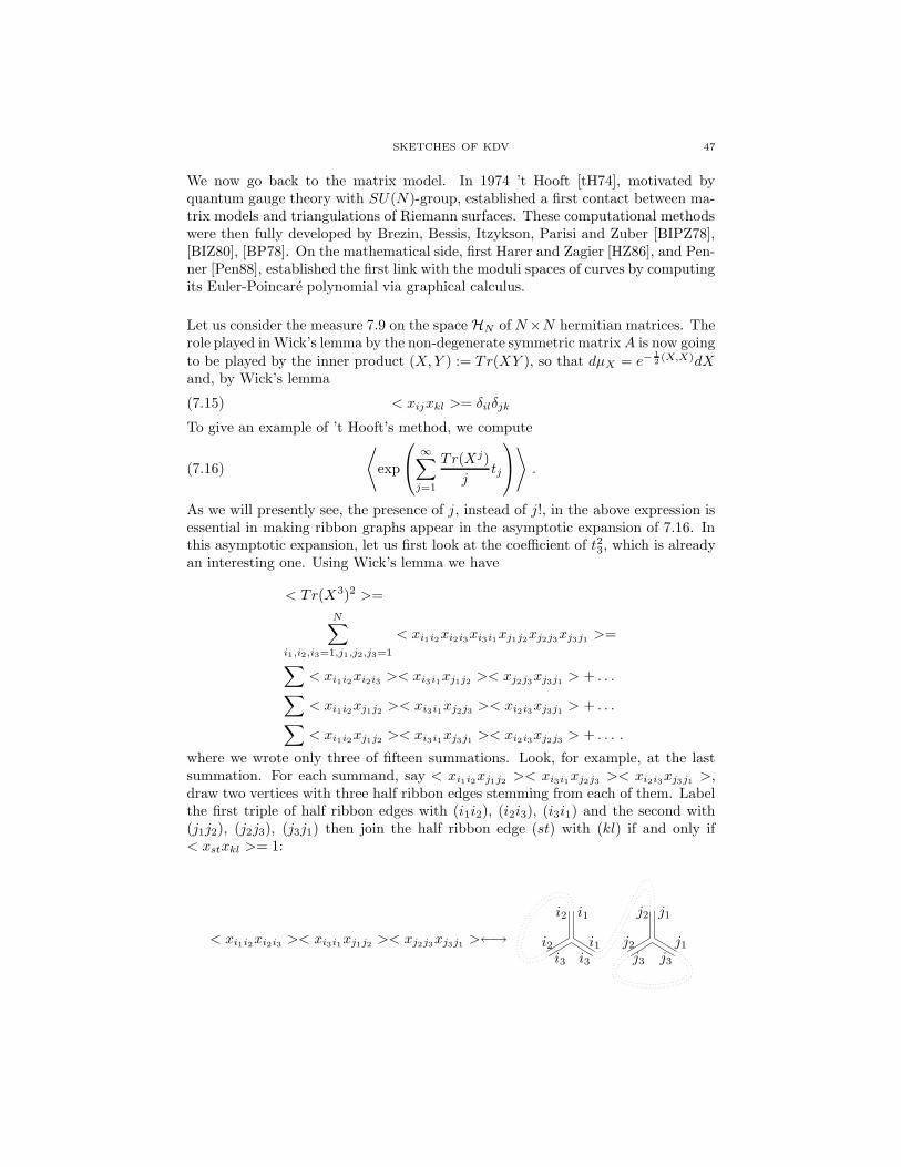
SKETCHES OF KDV 47

We now go back to the matrix model. In 1974 ’t Hooft [tH74], motivated byquantum gauge theory with SU(N)-group, established a first contact between ma-trix models and triangulations of Riemann surfaces. These computational methodswere then fully developed by Brezin, Bessis, Itzykson, Parisi and Zuber [BIPZ78],[BIZ80], [BP78]. On the mathematical side, first Harer and Zagier [HZ86], and Pen-ner [Pen88], established the first link with the moduli spaces of curves by computingits Euler-Poincare polynomial via graphical calculus.

Let us consider the measure 7.9 on the space HN of N×N hermitian matrices. Therole played in Wick’s lemma by the non-degenerate symmetric matrixA is now going

to be played by the inner product (X,Y ) := Tr(XY ), so that dµX = e−12 (X,X)dX

and, by Wick’s lemma

(7.15) < xijxkl >= δilδjk

To give an example of ’t Hooft’s method, we compute

(7.16)

⟨exp

∞∑

j=1

Tr(Xj)

jtj

⟩.

As we will presently see, the presence of j, instead of j!, in the above expression isessential in making ribbon graphs appear in the asymptotic expansion of 7.16. Inthis asymptotic expansion, let us first look at the coefficient of t23, which is alreadyan interesting one. Using Wick’s lemma we have

< Tr(X3)2 >=

N∑

i1,i2,i3=1,j1,j2,j3=1

< xi1i2xi2i3xi3i1xj1j2xj2j3xj3j1 >=

∑< xi1i2xi2i3 >< xi3i1xj1j2 >< xj2j3xj3j1 > + . . .

∑< xi1i2xj1j2 >< xi3i1xj2j3 >< xi2i3xj3j1 > + . . .

∑< xi1i2xj1j2 >< xi3i1xj3j1 >< xi2i3xj2j3 > + . . . .

where we wrote only three of fifteen summations. Look, for example, at the lastsummation. For each summand, say < xi1i2xj1j2 >< xi3i1xj2j3 >< xi2i3xj3j1 >,draw two vertices with three half ribbon edges stemming from each of them. Labelthe first triple of half ribbon edges with (i1i2), (i2i3), (i3i1) and the second with(j1j2), (j2j3), (j3j1) then join the half ribbon edge (st) with (kl) if and only if< xstxkl >= 1:

< xi1i2xi2i3 >< xi3i1xj1j2 >< xj2j3xj3j1 >←→

i2

i2

i1

i1i3 i3

j2

j2

j1

j1j3 j3

48 ENRICO ARBARELLO

We get the following ribbon graphs (one of genus 1 and two of genus 0):

In the sum above, nine summands give a graph of type (a), three of type (b) andthree of type (c). Notice that each of the above two ribbon graphs is coloured ,meaning that each boundary component is coloured with a colour i ∈ 1, . . . , N.Hence < Tr(X3)2 >= 12N3 + 3N . The coefficient of t23 , in the asymptotic ex-

pansion of 7.16, is equal to <Tr(X3)2>18 = N3

2 + N3

6 + N6 and this is nice, since the

automorphism group of a graph of type (a) is cyclic of order 2 while the automor-phism group of a graph of type (b) or (c) is

3. The general formula is

(7.17)

⟨exp

∞∑

j=1

Tr(Xj)

jtj

⟩

∑

Γ∈G

N b(Γ)

|Aut(Γ)|∏

j≥1

tνj(Γ)j ,

where G is the set of isomorphism classes of ribbon graphs and νj(Γ) is the numberof j-valent vertices of Γ and b(Γ) is the number of its boundary components.

The connection between ribbon graphs and moduli spaces of curves is provided bya remarkable theorem by Strebel [Str84]. The theorem states that, given a smoothn-pointed, genus g curve (C, x1, . . . , xn), with n ≥ 1, and n positive real numbersa1, . . . , an there exists a unique quadratic differential ω, called a Jenkins-Strebel

differential, having the following properties. First, the non-critical horizontal tra-jectories of ω are closed. Secondly, if Γ is the union of all the critical trajectories,

then C \ Γ is the union af n discs ∆1, . . . ,∆n and ω = − ai

2πdz2

z2 in ∆i. One couldimagine that the surface C is made of water and that one is throwing n stones ofdifferent weights producing circular waves mutually interfering along Γ.

•

•

−→

.

.

.

.

.

.

.

.

.

.

.

.

.

.

.

.

.

.

.

.

.

.

.

.

.

.

.

.

.

.

.

.

.

.

.

.

.

.

.

.

.

.

.

.

.

.

.

..

The orientation of C gives Γ the structure of a connected ribbon graph. The verticesof Γ correspond to the zeros of ω: a ν-valent vertex of Γ corresponds to a zero oforder ν − 2 of ω. The metric induced by |ω| on C, is smooth and flat everywhereexcept at the zeros of ω. In this metric, the punctured disc ∆i \ xi appears as aninfinite cylinder whose parallels are the horizontal trajectories of ω which are circlesof ω-length equal to ai. The Jenkins-Strebel differential ω can thus be thought of as

SKETCHES OF KDV 49

a way of discretizing the metric of C by concentrating the curvature on the verticesof Γ.

Mumford realized, in the early 80’s, that Jenkins-Strebel differentials offered abeautiful way of defining a cellular decomposition of Mg,n or, rather, of Mg,n× n+ .Given a point y = (C, x1, . . . , xn, a1, . . . , an) ∈Mg,n× n+ , take the Jenkins-Strabeldifferential ω associated to it and look at its critical graph Γ equipped with itsω-metric. Then the point y can be viewed as a point of the orbi-cell

eΓ := l(Γ)+ /Aut(Γ)

where l(Γ) is the number of sides of Γ. Moving from one cell to another of smaller(resp. bigger) dimension corresponds to the contraction of a side (resp. the ex-pansion of a vertex) i.e. to a Feynman move. Moving around on a cell eΓ justmeans changing the ω-length of the sides of Γ. Using this cell decomposition andan appropriate matrix model, Harer and Zagier, and then Penner, computed thevirtual Euler-Poincare characteristic of Mg,n which is defined by

χvirt(Mg,n) =∑

Γ∈Gg,n

(−1)l(Γ)

Aut(Γ),

where Gg,n is the set of isomorphism classes of ribbon graphs of genus g with nboundary components. Kontsevich, in proving Witten’s conjecture, shows that asimilar method can be used to compute the intersection numbers < τd1 , . . . τdn

>.

The Kontsevich matrix model. One of the basic steps in Kontsevich’s proofof Witten’s conjecture is to reduce the computation of the intersection numbers7.1 or, better, of the partition function 7.2, to the graphical calculus based on aspecific matrix model. The matrix model proposed by Kontsevich is based on theprobability distribution

dµΛ,X = exp(−1

2TrΛX2)dX ,

where Λ = diag(Λ1, . . . ,ΛN ) is a real non-singular diagonal matrix. The elementarycorrelators for this probability distribution are given by

< xij , xkl >Λ= δilδjk2

Λi + Λj

The first result proved by Kontsevich is that Witten’s partition function 7.3 can beexpressed as a matrix integral in the asymptotic form

(7.18) Z(t0(Λ), t1(Λ), . . . ) Λ−1→0

⟨exp

(√−1

6TrX3

)⟩

Λ

where

ti(Λ) = −(2i− 1)!!TrΛ−(2i−1) ,

and where < >Λ denotes the expectation value with respect to dµΛ,X . To prove7.18 the first step is to give a combinatorial expression of the (3g − 3 + n)-form

ψd11 · · ·ψdnn on a cell eΓ of maximal dimension. It turns out that if lj1 , . . . , ljki

50 ENRICO ARBARELLO

are the successive lengths of the i-th boundary component of Γ, numbered in thecounterclockwise way, and if pi = lj1 + · · · + ljki

then

ωi := ψi|eΓ =∑

1≤µ<ν≤ki−1

d

(ljµpi

)∧ d(ljνpi

).

Setting d = 3g− 3 + n, and looking at a fiber q−1(p∗) of q : Mg,n × n+ → n+ , oneobtains

∫

q−1(p∗)

(∑p2iωi)

d

d!=

∑∑di=d

< τd1 , . . . , τdn>

n∏

i=1

p2di

i

di!.

Taking the Laplace transform of both sides, i.e. intergrating along n+ against∏ni=1 dpie

−λipi , one obtains

∫

Mg,n×

n+

n∏

i=1

dpie−λipi

((∑p2iωi)

d

d!

)=

∑∑di=d

< τd1 , . . . , τdn>

∫ ∞

0

n∏

i=1

dpie−λipi

(p2di

i

di!

)=

∑∑di=d

< τd1 , . . . , τdn>

n∏

i=1

(2di − 1)!!λ−(2di+1)i .

Clearly there must be a constant c such that

1

d!

n∏

i=1

dpi ∧

n∑

i=1

∑

1≤µ<ν≤ki−1

d liµ ∧ d liν

d

= c · d l1 ∧ · · · ∧ dll(Γ) .

where l(Γ) is the number of edges of Γ. The innocent-looking computation of thisconstant turns out to be highly non-trivial and gives

c = 2(5g−5+2n) .

From this it is not too hard to show (see [Kon92] ) that

∑

3g−3+n=d

< τd1 , . . . , τdn>

n∏

i=1

(2di − 1)!!λ−(2di+1)i =

∑

Γ∈Gcg,n,3

2v(Γ)

|Aut(Γ)|∏

e∈E(Γ)

2

λi(e) + λi′(e),

where Gcg,n,3 is the set of isomorphism classes of connected trivalent ribbon graphsof genus g with n boundary components, E(Γ) is the set of edges of Γ and, for eachedge e, the indices of the boundary components on the two sides of e are i(e) andi′(e). But now, the graphical calculus of matrix integral we discussed above gives,

SKETCHES OF KDV 51

after some computations 12

(7.19)

Z(t0(Λ), t1(Λ), . . . ) =∑

g≥0,n≥12−2g−n<0

∑

Γ∈Γg,n,3

2v(Γ)

|Aut(Γ)|∏

e∈E(Γ)

2

λi(e) + λi′(e)

Λ−1→0N→∞

∫HN

e√

−16 TrX3− 1

2TrΛX2

dX∫HN

e−12TrΛX

2dX

=

⟨exp

(√−1

6TrX3

)⟩

Λ

as desired. In the last formula Γg,n,3 is the set of isomorphism classes of tr ivalent,N -coloured, ribbon graphs of genus g, with n boundary components (see [Loo93],[Kon92]).

In each of the above formulae, whenever the symbol |Aut(Γ)| appears in a sum-mation over a certain set S of graphs, one should understand that Aut(Γ) is theautomorphism group of the (ribbon) graph Γ equipped with the extra structuredescribed in the definition of S ( coloured, numbered, etc.): a remarkable fact.

The connection with KdV. The first link between the matrix model and theKdV was found in 1989-90 through the works by Kazakov [Kaz89], Brezin-Kazakov[BK90], Douglas [Dou90], Douglas-Shenker [DS90], Gross-Migdal [GM90], whereit was discovered that the matrix model could be used to give a non-perturbativedescription of 2D gravity. The partition function of this matrix model is of type

Z(β) =

∫

HN

eβTrV (X)dX,

where V (X) =∑giX

i is some potential. To evaluate these integrals one may usethe method of orthogonal polynomials (see [Kak00] p.357) and then the discreteToda lattice makes its appearence. Passing from a discrete to a continuous param-eter, one gets the KdV equation. More or less at the same time Witten, Dijkgraaf,Verlinde and Verlinde [Wit91], [DW90], [DVV91], [Dij92], discoverd that the samepartition function arises in 2D topological gravity. But here a new feature makesits appearence. The string equation and the KdV equation appear, so to speak, on

12 Here one uses a standard trick: exponentiating a sum over connected (ribbon) graphs oneobtains a sum over all (ribbon) graphs.

52 ENRICO ARBARELLO

equal footing, by virtue of certain Virasoro operators. This lead Witten to give thefollowing formulation of his conjecture.

Consider the operators

L−1 = − ∂

∂t0+

∞∑

i=1

ti∂

∂ti−1+t202

L0 = −3 · ∂

∂t1+

∞∑

i=0

(2i+ 1)ti∂

∂ti+

1

8

L1 = −5 · 3 · ∂

∂t2+

∞∑

i=0

(2i+ 1)(2i+ 3)ti∂

∂ti+1+

1

2

∂2

∂t20

L2 = −7 · 5 · 3 · ∂

∂t3+

∞∑

i=0

(2i+ 1)(2i+ 3)(2i+ 5)ti∂

∂ti+2+ 3

∂2

∂t0∂t1

. . . . . . . . .

Lk = −(2k + 3)!! · ∂

∂tk+1+

∞∑

i=0

(2k + 2i+ 1)!!

(2i− 1)!!ti

∂

∂ti+k+

+1

2

∑

r+s+1=k

(2r + 1)!!(2s+ 1)!!∂2

∂tr∂ts,

then the partition function 7.3 satisfies

(7.20) LnZ = 0 , for n ≥ −1 .

The fact that the equations 7.20 are equivalent to the string equation 7.4 togetherwith the Gelfand-Dikii equations 7.5, rests on three facts. On the equality:

∂2

∂t20(Z−1Ln+1Z) =

1

2n+ 1

(∂U

∂t0

∂

∂t0+ 2U

∂2

∂t20+

1

4

∂4

∂t40

)(Z−1LnZ) , n ≥ −1 ,

on the Virasoro relation:

(7.21) [Lm, Ln] = (m− n)Lm+n ,

and on the uniqueness of the solution to 7.4 and 7.5 (see [Wit92], [Get99] for details).

The equivalence between the Virasoro equations 7.20, on one side, and the stringequation 7.4 together with the Gelfand-Dikii equations 7.5, on the other , is thereflection of the following strong symmetry property of the solution Z to 7.20.Think of Z as a τ -function and, via the boson-fermion correspondence, look at itscorresponding point [WZ ] ∈ Gr0(H). Since Z satisfies the KdV, the subspaceWZ isinvariant under multiplication by z2. This is the first (trivial) symmetry. But usingthe matrix-integral expression for Z, one can show that WZ ⊂ H =

[[z]][z−1 ] is

also invariant under the action of certain operators An,with n ≥ −1, defined by:An = 1

2z2n+2A, where

(7.22) A = −z−1 d

dz+

1

2z−2 + z.

SKETCHES OF KDV 53

The operators An satisfy the Virasoro relations: [Am, An] = (m − n)Am+n. Now,as Kac and Schwarz show [KS91], the symmetry conditions

(7.23) λ2WZ ⊂WZ , AnWZ ⊂WZ ,

translate, via the boson-fermion correspondence, into the equations 7.20. An es-sential feature of the symmetry property 7.23 is the fact that the operators A2 andz2 coincide on WZ :

(7.24) (A2 − z2)∣∣WZ

= 0 .

This is equivalent to the the classical Airy equation: f ′′(t)+ tf(t) = 0. One can seethat the Airy equation 7.24 directly connects with the Kontsevich’s matrix modelby observing that the partition function for the N = 1 case and for z = Λ is:

Z(Λ) =

⟨exp

(√−1

6X3

)⟩

Λ

=

∫∞

−∞ e√

−16 X3− 1

2 ΛX2

dX∫∞

−∞e−

12 ΛX2

dX

=∞∑

k=0

(−2

9

)k Γ(3k + 12 )

(2k!)√π

Λ−3k

and satisfies (A2 − Λ2)Z(Λ) = 0 (see [IZ92]) . In a sense, this observation isthe starting point of the proof that the partition function Z(Λ) for Kontsevich’sN -matrix model satisfies the KdV equation. In fact, for general N , Konstevichreduces the KdV hierachy to a matrix version of the Airy equation.

Just after Kontsevich proved Witten’s conjecture in its original form, Witten in[Wit92] went back to 7.20 and proved it using Kontsevich’s main identity 7.19. Thefirst two equations L−1Z = 0 and L0Z = 0 were already proved quite beautifullyby algebraic-geometrical methods in [Wit91], pp.255,256 . The second one, forexample, is really easy. It reduces to the following relation among the coefficientsof Z: < τ1τd1 , . . . , τdn

>= (2g − 2 + n) < τd1 , . . . , τdn>, which is obtained by

integration along the fibers of π : Mg,n+1 → Mg,n. This looks very promisingbecause, since the operators Ln satisfy the Virasoro relation: [Lm, Ln] = (m −n)Lm+n, to prove 7.20 one is reduced to prove the single relation L2Z = 0. But,unfortunately, this relation seems to elude any direct, algebro-geometrical proofalong the lines used by Witten to prove L−1Z = L0Z = 0 .

On the other hand, Witten looks at the partition function in matrix form

Z(t0(Λ), t1(Λ), . . . ) =

⟨exp

(√−1

6TrX3

)⟩

Λ

and, by taking derivatives under the integral sign, he shows directly that

(∞∑

i=0

(2i+ 1)(2i+ 3)(2i+ 5)ti∂

ti+2

)Z =

⟨i

64TrX7 +

3

16TrX3TrX − i

8TrX

⟩.

54 ENRICO ARBARELLO

Then, using graphical calculus, he shows that

∂2Z

∂t0∂t1=

⟨1

12TrX3TrX − i7

4TrX

⟩

3 · 5 · 7 · ∂Z∂t3

=

⟨i

64TrX7 +

7

16TrX3TrX − i

8TrX

⟩,

thus verifying that L2Z = 0.

Actually, as conjectured by both Witten and Kontsevich, the above computationis part of a broader picture which, subsequently, was completely described by DiFrancesco Itzykson and Zuber. Using only algebraic methods, they give, in [FIZ93],an explicit bijection

φ : [∂

∂t0,∂

∂t1,∂

∂t2, . . .

]→

[TrX, TrX3, T rX5 , . . .

]

such that

P

(∂

∂t0,∂

∂t1, . . .

)⟨exp

(√−1

6TrX3

)⟩

Λ

=

⟨φ(P )

(TrX, TrX3, . . .

)exp

(√−1

6TrX3

)⟩

Λ

,

obtaining as a biproduct 7.20. Their results have been revisited in[FM01b] fromthe point of view of graphical calculus.

It is interesting to notice that the initial value of the KdV hierachy satisfied by Zis

∂2 + 2t0, where 2t0 =∂2 logZ

∂t20(t0, 0, 0 . . . ) ,

and that the ring AWZ, (cf. 5.11), is just the ring of constants: AWZ

=

, so thatthe partition function Z for the intersection numbers on moduli spaces of curves isfar from being algebro-geometric solution of KdV.

Sources: In adddition to the original papers by Witten and Kontsevich [Wit91],[Kon92], there are a number of papers presenting Witten’s conjecture and (varia-tions of) Kontsevich’s solution of it . Among them are: [Loo93], [IZ92], [Wit92],[FIZ93]. An alternative proof of Kontsevich’s main identity 7.19 has been given in[PO01] using the asymptotics of Hurwitz numbers. From a physical point of view,the origin of the conjecture and of the link between matrix model and KdV, canbe found in the book by Kaku [Kak00].

Possible references regarding random matrices, are the classical book of Mehta[Met91], and [Dei00], [Ble99], [ASvM95], [Oko00a].

The following papers study matrix models: [BIZ80], [Mul95], [Mul94b], [Fra99],[Zvo97], [FM01a].

A description of how Strebel’s theorem defines a cell decomposition of Teichmuller’sspace Tn,g (and an orbi-cell decomposition of Mg,n), is contained in [Loo95].

SKETCHES OF KDV 55

The interplay between matrix models, non-linear differential equations of KdV typeand enumerative geometry is one of the most fruitful developments of the recentyears. A central conjecture in the intersection theory of projective varieties is the socalled Virasoro conjecture due to Eguchi, Hori and Xiong [EHX97]. This conjecturepredicts that the partition function ZV for the quantum cohomology of a smoothprojective variety V (see [Man99]) satisfies Virasoro constraints LiZV = 0 , i ≥ −1 ,which generalize the ones we discussed in our presentation of Witten’s conjecture(in Witten’s case the target variety V consists of a single point). An overview of theconjecture by Eguchi, Hori and Xiong’s is given in [Get99]. Progress in solving thisconjecture have been made by Liu-Tian [LT98], by Dubrovin-Zhang [AD98] andby Givental [?]. When the target variety is the projective line 1, the conjectureis naturally linked to the classical Hurwitz numbers counting ramified covers of 1 of given degree and with prescribed configuration of the ramification locus (see[ELSV99], [FP99]). As it was discovered in [EY94] and [Hor95], it is the Todaequation, instead of the KdV, that makes its appearence in this circle of ideas.A systematic study of the Gromov-Witten invariants of 1 has been initiated in[PO01] (see also [Oko00b], [Pan00]).

References

[AC84] E. Arbarello and C. De Concini. On a set of equations characterizing Riemann ma-trices. Ann. of Math., 2(120):119–140, 1984.

[AC90] E. Arbarello and C. De Concini. Geometrical aspects of the Kadomtsev-Petviashviliequation. In Global geometry and mathematical physics (Montecatini Terme, 1988),pages 95–137. Springer, Berlin, 1990.

[AC91] E. Arbarello and C. De Concini. Abelian varieties, infinite-dimensional Lie algebras,and the heat equation. In Complex geometry and Lie theory (Sundance, UT, 1989),pages 1–31. Amer. Math. Soc., Providence, RI, 1991.

[ACGH85] E. Arbarello, M. Cornalba, P. A. Griffiths, and J. Harris. Geometry of AlgebraicCurves. Springer, Berlin, 1985. Vol I.

[ACKP88] E. Arbarello, C. De Concini, V. G. Kac, and C. Procesi. Moduli spaces of curves andrepresentation theory. Comm. Math. Phys., 117(1):1–36, 1988.

[AD98] B. A. and Dubrovin. Bi-hamiltonian hierarchies in 2D topological field theory atone-loop approximation. Compositio Math., 111(2):167–219, 1998.

[Adl79] M. Adler. On a trace functional for formal pseudo differential operators and the sym-plectic structure of the Korteweg-de Vries type equations. Invent. Math., 50(3):219–248, 1978/79.

[AMM77] H. Airault, H. P. McKean, and J. Moser. Rational and elliptic solutions of theKorteweg-de Vries equation and a related many-body problem. Comm. Pure Appl.Math., 30(1):95–148, 1977.

[Arb87] E. Arbarello. Periods of abelian integrals, theta functions, and differential equationsof KdV type. In Proceedings of the International Congress of Mathematicians, Vol.1, 2 (Berkeley, Calif., 1986), pages 623–627, Providence, RI, 1987. Amer. Math. Soc.

[ASvM95] M. Adler, T. Shiota, and P. van Moerbeke. Random matrices, vertex operators andthe Virasoro algebra. Phys. Lett. A, 208(1-2):67–78, 1995.

56 ENRICO ARBARELLO

[AvM80] M. Adler and P. van Moerbeke. Completely integrable systems, Euclidean Lie alge-bras, and curves. Adv. in Math., 38(3):267–317, 1980.

[BC23] J. L. Burchnall and T. W. Chaundy. Commutative ordinary differential operators.Proc. London Math. Soc. Ser 2, 21:420–440, 1923.

[BC28] J. L. Burchnall and T. W. Chaundy. Commutative ordinary differential operators.Proc. Royal Soc. Ser A, 118:557–583, 1928.

[Bea90] A. Beauville. Jacobiennes des courbes spectrales et systemes hamiltonienscompletement integrables. Acta Math., 164(3-4):211–235, 1990.

[BIPZ78] E. Brezin, C. Itzykson, G. Parisi, and J. B. Zuber. Planar diagrams. Comm. Math.Phys., 59(1):35–51, 1978.

[BIZ80] D. Bessis, C. Itzykson, and J. B. Zuber. Quantum field theory techniques in graphicalenumeration. Adv. Appl. Math., 1(2):109–157, 1980.

[BK90] E. Brezin and V. A. Kazakov. Exactly solvable field theories of closed strings. Phys.Lett. B, 236(2):144–150, 1990.

[Ble99] P. M. Bleher. In “Random matrix models and their applications”. Mathematical Sci-ences Research Institute, Berkeley, CA, 1999. Lectures from the workshop held inBerkeley, CA, February 22–26, 1999.

[BM86] A. A. Beılinson and Yu. I. Manin. The Mumford form and the Polyakov measure instring theory. Comm. Math. Phys., 107(3):359–376, 1986.

[BMS87] A. A. Beılinson, Yu. I. Manin, and V. V. Schechtman. Sheaves of the Virasoroand Neveu-Schwarz algebras. In K-theory, arithmetic and geometry (Moscow, 1984–1986), pages 52–66. Springer, Berlin, 1987.

[BNS96] I. Biswas, S. Nag, and D. Sullivan. Determinant bundles, Quillen metrics and Mum-ford isomorphisms over the universal commensurability Teichmuller space. ActaMath., 176(2):145–169, 1996.

[BP78] E. Brezin and G. Parisi. Critical exponents and large-order behavior of perturbationtheory. J. Statist. Phys., 19(3):269–292, 1978.

[BS88] A. A. Beılinson and V. V. Schechtman. Determinant bundles and Virasoro algebras.

Comm. Math. Phys., 118(4):651–701, 1988.[CD82] F. Calogero and A. Degasperis. Spectral transform and solitons. Vol. I. North-Holland

Publishing Co., Amsterdam, 1982. Tools to solve and investigate nonlinear evolutionequations, Lecture Notes in Computer Science, 144.

[DEGM82] R. K. Dodd, J. C. Eilbeck, J. D. Gibbon, and H. C. Morris. Solitons and nonlinearwave equations. Academic Press Inc. [Harcourt Brace Jovanovich Publishers], London,1982.

[Dei96] P. Deift. Integrable Hamiltonian systems. In Dynamical systems and probabilisticmethods in partial differential equations (Berkeley, CA, 1994), pages 103–138. Amer.Math. Soc., Providence, RI, 1996.

[Dei00] P. Deift. Orthogonal Polynomials, and Random Matrices: A Riemann-Hilbert Ap-proach. American Mathematical Society. Courant Lecture Notes 3, Providence, RI,2000.

[Dic91] L. A. Dickey. Soliton equations and Hamiltonian systems. World Scientific PublishingCo. Inc., River Edge, NJ, 1991.

[Dij92] R. Dijkgraaf. Intersection theory, integrable hierarchies and topological field theory.In New symmetry principles in quantum field theory (Cargese, 1991), pages 95–158.Plenum, New York, 1992.

[DKJM83] E. Date, M. Kashiwara, M. Jimbo, and T. Miwa. Transformation groups for soli-ton equations. In Nonlinear integrable systems—classical theory and quantum theory(Kyoto, 1981), pages 39–119. World Sci. Publishing, Singapore, 1983.

[DMN76] B. A. Dubrovin, V. B. Matveev, and S. P. Novikov. Nonlinear equations of Korteweg-de Vries type, finite-band linear operators and Abelian varieties. Uspehi Mat. Nauk,31(1(187)):55–136, 1976.

[Dou90] M. R. Douglas. Strings in less than one dimension and the generalized KdV hierar-chies. Phys. Lett. B, 238(2-4):176–180, 1990.

[Dra83] P. G. Drazin. Solitons. Cambridge University Press, Cambridge, 1983. London Math-ematical Society Lecture Notes.

[DS85] V. G. Drinfeld and V. V. Sokolov. Lie algebras and equation of KdV type. J. Sov.Math., 30:1975–20361, 1985.

SKETCHES OF KDV 57

[DS90] M. R. Douglas and S. H. Shenker. Strings in less than one dimension. Nuclear Phys.B, 335(3):635–654, 1990.

[DT80] P. Deift and E. Trubowitz. Some remarks on the Korteweg-de Vries and Hill’s equa-tions. In Nonlinear dynamics (Internat. Conf., New York, 1979), pages 55–64. NewYork Acad. Sci., New York, 1980.

[Dub75] B. A. Dubrovin. The periodic problem for the korteweg de vries equation in a classof finite zone potentials. Funct, Anal. Appl., 9:215–222, 1975.

[Dub81] B. A. Dubrovin. Theta-functions and nonlinear equations. Uspekhi Mat. Nauk,36(2(218)):11–80, 1981. With an appendix by I. M. Krichever.

[Dub82] B. A. Dubrovin. The Kadomcev-Petviashvilii equation and the relations between theperiods of holomorphic differentials on Riemann Surfaces. Math. USSR-Izv, 19:205–217, 1982.

[DVV91] R. Dijkgraaf, E. Verinde, and H. Verlinde. Loop equations and Virasoro constarintsin nonperturbative two-dimensional quantum gravity. Nucl. Phys. B, B 348:435–456,1991.

[DW90] R. Dijkgraaf and E. Witten. Mean field theory, topological field theory, and multi-matrix models. Nuclear Phys. B, 342(3):486–522, 1990.

[EHX97] T. Eguchi, K. Hori, and C.-S. Xiong. Quantum cohomology and Virasoro algebra.Phys. Lett. B, 402(1-2):71–80, 1997.

[ELSV99] T. Ekedahl, S. Lando, M. Shapiro, and A. Vainshtein. On Hurwitz numbers andHodge integrals. C. R. Acad. Sci. Paris Ser. I Math, 328(12):1175–1180, 1999.

[EY94] T. Eguchi and S.-K. Yang. The topological CP 1 model and the large N matrix inte-gral. Mod. Phys. Lett., A9:2893–2902, 1994.

[Fad63] L. D. Faddeev. The inverse problem in quantum theory of scattering. J. Math. Phys.,4:72–104, 1963.

[FIZ93] P. Di Francesco, C. Itzykson, and J.-B. Zuber. Polynomial averages in the Kontsevichmodel. Commun. Math. Phys., 151:193–219, 1993.

[FM78a] H. Flaschka and D. W. McLaughlin. Introduction to mathematical techniques forcontinuous problems. Rocky Mountain J. Math., 8(1-2):3–14, 1978. Conference onthe Theory and Application of Solitons (Tucson, Ariz., 1976).

[FM78b] H. Flaschka and D. W. McLaughlin. Introduction to waves in plasmas. Rocky Moun-tain J. Math., 8(1-2):253–255, 1978. Conference on the Theory and Application ofSolitons (Tucson, Ariz., 1976).

[FM01a] D. Fiorenza and R. Murri. Feynman diagrams for mathematicians. 2001. Preprint,Roma, “La Sapienza”.

[FM01b] D. Fiorenza and R. Murri. Matrix Integrals and Feynman Diagrams in the KontsevichModel. 2001. Preprint.

[FP99] B. Fantechi and R. Pandharipande. Stable maps and branch divisors. 1999. Preprint.[FPU55] E. Fermi, J. R. Pasta, and S. M. Ulam. Studies of nonlinear problems. pages 978–988,

1955. in Collected works of Enrico Fermi, vol II, Chicago University Press.[Fra99] P. Di Francesco. 2-D quantum and topological gravities, matrix models, and integrable

differential systems. In The Painleve property, pages 229–285. Springer, New York,1999.

[GD75] I. M. Gel′fand and L. A. Dikiı. Asymptotic properties of the resolvent of Sturm-Liouville equations, and the algebra of Korteweg-de Vries equations. Uspehi Mat.Nauk, 30(5(185)):67–100, 1975.

[GD76] I. M. Gel’fand and L. A. Dikii. Fractional powers of operators and Hamiltonian sys-tems. Funct. Anal. Appl., (10):259–273, 1976.

[Get99] E. Getzler. The Virasoro conjecture for Gromov-Witten invariants. In Algebraic geom-etry: Hirzebruch 70 (Warsaw, 1998), pages 147–176. Amer. Math. Soc., Providence,RI, 1999.

[GM90] D. J. Gross and A. A. Migdal. A nonperturbative treatment of two-dimensional quan-tum gravity. Nuclear Phys. B, 340(2-3):333–365, 1990.

[GMKM67] C. S. Gardner, Green J. M., M. D. Kruskal, and R. M. Miura. Method for solving theKorteveg de Vries equation. Phys. Rev. Lett., (19):1095–1097, 1967.

[GMKM75] C. S. Gardner, Green J. M., M. D. Kruskal, and R. M. Miura. Korteveg de Vriesequation and generalizations.VI. Methods for exact solutions. Comm. Pure Appl.Math., 27:97–133, 1975.

58 ENRICO ARBARELLO

[Gri85] P. A. Griffiths. Linearizing flows and a cohomological interpretation of Lax equations.Amer. J. Math., 107(6), 1985.

[Gro84] A. Grothendieck. Esquisse d’un programme. 1984. Preprint.[Gun82] R. C. Gunning. Some curves in abelian varieties. Invent. Math., 66(3):377–389, 1982.[Har83] J. Harer. The second homology group of the mapping class group of an orientable

surface. Invent. Math., 72(2):221–239, 1983.[Hir71] R. Hirota. Exact solutions of the Korteveg de Vries equation for multiple collision of

solitons. Phys. Rev. Lett., 27:1192–1194, 1971.[Hir76] R. Hirota. Direct methods of finding exact solutions of nonlinear evolution equations.

Lect. Notes in Math. Springer, 515:40–68, 1976. in Backlund transformations, inversescatteringmethods, solitons and their applications.

[Hor95] K. Hori. Constraints for topological strings in D ≥1. Nuclear Physics B, 439:395–420,1995.

[HZ86] J. Harer and D. Zagier. The Euler characteristic of the moduli space of curves. Invent.Math., 85(3):457–485, 1986.

[Inc56] E. L. Ince. Ordinary differential equations. Dover, New York, 1956.[IZ92] C. Itzykson and J.-B. Zuber. Combinatorics of the modular group II, the Kontsevich

integrall. Int. J. Mod. Phys., A 7:5661–5705, 1992.[Kac90] V. Kac. Infinite dimensional Lie algebras. Cambridge Univerity Press, Cambridge,

3rd edition, 1990.[Kak00] M. Kaku. Strings, conformal fields, and M-Theory. Second edition. Graduate text in

Contemporary Physics. Springer Verlag, New York, 2000.[Kaz89] V. A. Kazakov. The appearance of matter fields from quantum fluctuations of 2D-

gravity. Modern Phys. Lett. A, 4(22):2125–2139, 1989.[Kd95] D. J. Korteweg and G. de Vries. On the change of form of long waves advancing in a

rectangular canal, and on a new type of long stationary waves. Phil. Mag., 39:422–443,1895.

[KNTY88] N. Kawamoto, Y. Namikawa, A. Tsushija, and Y. Yamada. Geometric realizationof conformal field theory on Riemann surfaces. Commun. Math Phys., 116:247–308,1988.

[Kon87] M. Kontsevich. Virasoro algebra and Teicmuller spaces. Funct. Anal. Appl., 21(2):78–79, 1987.

[Kon92] M. Kontsevich. Intersection theory on the moduli space of curves and the matrix Airyfunction. Commun. Math. Phys., 147:1–23, 1992.

[KP70] B. B. Kadomtsev and V. I. Petviashvili. On the stability of solitary waves in weaklydispersive media. Sov. Phys. Doklady, 15:539–541, 1970.

[KR87] V. G. Kac and A. K. Raina. Bombay lectures on highest weight representations ofinfinite-dimensional Lie algebras. World Scientific Publishing Co. Inc., Teaneck, NJ,1987.

[Kri77a] I. M. Krichever. Integration of non-linear equations by methods of algebraic geometry.Funct.Anal.Appl., 11(1):12–26, 1977.

[Kri77b] I. M. Krichever. Methods of algebraic geometry in the theory of non-linear equations.Russian Math. Surveys, 32(6):185–213, 1977.

[Kri78] I. M. Kricever. Commutative rings of ordinary linear differential operators. Funkt-sional. Anal. i Prilozhen., 12(3):20–31, 96, 1978.

[Kru78] M. Kruskal. The birth of the soliton. In Nonlinear evolution equations solvable bythe spectral transform (Internat. Sympos., Accad. Lincei, Rome, 1977), pages 1–8.Pitman, Boston, Mass., 1978.

[KS91] V. Kac and A. Schwartz. Geometric interpretation of the partition function of 2Dgravity. Phys. Lett. B, 257:329–334, 1991.

[KW81] B. A. Kupershmidt and G. Wilson. Modifying Lax equations and the second Hamil-tonian structure. Invent. Math., 62(3):403–436, 1981.

[Lax68] P. D. Lax. Integrals of nonlinear equations of evolution and solitary waves. Comm.Pure Appl. Math., 21:467–490, 1968.

[Lax75] P. D. Lax. Periodic solutions of the KdV equation. Comm. Pure Appl. Math., 28:141–188, 1975.

[Lax76] P. D. Lax. Almost periodic solutions of the KdV equation. SIAM Rev., 18(3):351–375,1976.

SKETCHES OF KDV 59

[Lax78] P. D. Lax. A Hamiltonian approach to the KdV and other equations. In Nonlinearevolution equations (Proc. Sympos., Univ. Wisconsin, Madison, Wis., 1977), pages207–224. Academic Press, New York, 1978.

[Lax96] P. D. Lax. Outline of a theory of the KdV equation. In Recent mathematical methodsin nonlinear wave propagation (Montecatini Terme, 1994), pages 70–102. Springer,Berlin, 1996.

[Loo95] E. Looijenga. Cellular decompositions of compactified moduli spaces of pointedcurves. In The moduli space of curves (Texel Island, 1994), pages 369–400. BirkhauserBoston, Boston, MA, 1995.

[Loo93] E. Looijenga. Intersection theory on the Deligne-Mumford compactification.Seminaire Bourbaki, 45eme anneee(768):1–21, 1992-93.

[LT98] X. Liu and G. Tian. Virasoro constraints for quantum cohomology. J. DifferentialGeom., 50(3):537–590, 1998.

[Mag78] F. Magri. A simple model of the integrable Hamiltonian equation. J. Math. Phys.,19(5):1156–1162, 1978.

[Mag97] F. Magri. Eight lectures on integrable systems. In Integrability of nonlinear systems(Pondicherry, 1996), pages 256–296. Springer, Berlin, 1997.

[Mag98] F. Magri. The Hamiltonian route to Sato Grassmannian. In The bispectral problem(Montreal, PQ, 1997), pages 203–209. Amer. Math. Soc., Providence, RI, 1998.

[Man78] Yu. I. Manin. Algebraic aspects of nonlinear differential equations. In Current prob-lems in mathematics, Vol. 11 (Russian), pages 5–152. (errata insert). Akad. NaukSSSR Vsesojuz. Inst. Naucn. i Tehn. Informacii, Moscow, 1978.

[Man86] Yu. I. Manin. Quantum string theory and algebraic curves. 1986. Berkeley, ICM talk.[Man99] Yu. I. Manin. Frobenius manifolds, quantum cohomology and moduli spaces,. Ameri-

can Mathematical Society Publications, 47, Providence, RI, 1999.[Mar98] G. Marini. A geometrical proof of Shiota’s theorem on a conjecture of S. P. Novikov.

Compositio Math., 111(3):305–322, 1998.[McK80] H. P. McKean. Algebraic curves of infinite genus arising in the theory of nonlinear

waves. In Proceedings of the International Congress of Mathematicians (Helsinki,1978), pages 777–783, Helsinki, 1980. Acad. Sci. Fennica.

[McK81] H. P. McKean. Boussinesq’s equation on the circle. Comm. Pure Appl. Math.,34(5):599–691, 1981.

[McK84] H. P. McKean. Boussinesq’s equation: how it blows up. In J. C. Maxwell, the sesqui-centennial symposium (Amherst, Mass., 1981), pages 91–105. North-Holland, Ams-terdam, 1984.

[McK85] H. P. McKean. Variation on a theme of Jacobi. Comm. Pure Appl. Math., 38(5):669–678, 1985.

[Met91] Metha. Random Matrices. Academic, Boston, second edition edition, 1991.[MFK94] D. Mumford, J. Fogarty, and F. Kirwan. Geometric invariant theory. Springer-Verlag,

Berlin, third edition, 1994.[Miu76] R. M. Miura. The Korteveg de Vries equation: a survey of results. SIAM Rev.,

(18):412–459, 1976.[MM97] H. McKean and V. Moll. Elliptic curves. Cambridge University Press, Cambridge,

1997. Function theory, geometry, arithmetic.[Mos83] J. Moser. Integrable Hamiltonian systems and spectral theory. Scuola Normale Supe-

riore, Pisa, 1983.[MT78] H. P. McKean and E. Trubowitz. Hill’s surfaces and their theta functions. Bull. Amer.

Math. Soc., 84(6):1042–1085, 1978.[Mul83] M. Mulase. Algebraic geometry of soliton equations. Proc. Japan Acad. Ser. A Math.

Sci., 59(6):285–288, 1983.[Mul84] M. Mulase. Cohomological structure in soliton equations and Jacobian varieties. J.

Differential Geom., 19(2):403–430, 1984.[Mul94a] M. Mulase. Algebraic theory of the KP equations. In Perspectives in mathematical

physics, pages 151–217. Internat. Press, Cambridge, MA, 1994.[Mul94b] M. Mulase. Matrix integrals and integrable systems. In Topology, geometry and field

theory, pages 111–127. World Sci. Publishing, River Edge, NJ, 1994.[Mul95] M. Mulase. Asymptotic analysis of a Hermitian matrix integral. Internat. J. Math.,

6(6):881–892, 1995.

60 ENRICO ARBARELLO

[Mum78] D. Mumford. An algebro-geometric construction of commuting operators and of so-lutions to the Toda lattice equation, Korteweg de Vries equation and related nonlin-ear equation. In Proceedings of the International Symposium on Algebraic Geometry(Kyoto Univ., Kyoto, 1977), pages 115–153, Tokyo, 1978. Kinokuniya Book Store.

[Mum83a] D. Mumford. Tata lectures on theta. I. Birkhauser Boston Inc., Boston, MA, 1983.With the assistance of C. Musili, M. Nori, E. Previato and M. Stillman.

[Mum83b] D. Mumford. Towards an enumerative geometry of the moduli space of curves. pages271–328, 1983. in “Arithmetic and Geometry” (M. Artin and J. Tate, editors) vol 2Birkhauser, Boston.

[Mum84] D. Mumford. Tata lectures on theta. II. Birkhauser Boston Inc., Boston, MA, 1984.Jacobian theta functions and differential equations, With the collaboration of C.Musili, M. Nori, E. Previato, M. Stillman and H. Umemura.

[Mum99] D. Mumford. The red book of varieties and schemes. Springer-Verlag, Berlin, ex-panded edition, 1999. Includes the Michigan lectures (1974) on curves and their Ja-cobians, With contributions by Enrico Arbarello.

[MvM80] H. P. McKean and P. van Moerbeke. Hill and Toda curves. Comm. Pure Appl. Math.,33(1):23–42, 1980.

[Nov74] S. P. Novikov. The periodic problem for the Korteweg de Vries equation. FunctionalAnal. Appl., 8:236–246, 1974.

[Oko00a] A. Okounkov. Random matrices and random permutations. Internat. Math. Res.Notices, (20):1043–1095, 2000.

[Oko00b] A. Okounkov. Toda equations for Hurwitz numbers. Math. Res. Lett., 7(4):447–453,2000.

[Pan00] R. Pandharipande. The Toda equations and the Gromov-Witten theory of the Rie-mann sphere. Lett. Math. Phys., 53(1):59–74, 2000.

[Pen88] R. C. Penner. Perturbative series and the moduli space of Riemann surfaces. J. Dif-ferential Geom., 27(1):35–53, 1988.

[PO01] R. Pandharipande and A. Okounkov. Gromov-Witten theory, Hurwitz numbers, andmatrix models, I. pages 1–106, 2001. Preprint.

[Pol81] A. M. Polyakov. Quantum geometry of fermionic strings. Phys. Lett. B, 103(3):211–213, 1981.

[Pre96] E. Previato. Seventy years of spectral curves: 1923–1993. In Integrable systems andquantum groups (Montecatini Terme, 1993), pages 419–481. Springer, Berlin, 1996.

[Rai89] A. K. Raina. Fay’s trisecant identity and conformal field theory. Comm. Math. Phys.,122(4):625–641, 1989.

[Sat81] M. Sato. Soliton equations as dynamical systems on an infinite dimensional Grass-mannian manifold. Kokyuroku, Res. Inst. Math. Sci. Kyoto Univ., (439):30–46, 1981.

[Shi86] T. Shiota. Characterization of Jacobian varieties in terms of soliton equations. Invent.Mat., 83:333–382, 1986.

[SS80] V. V. Sokolov and A. B. Sabat. (L, A)-pairs and Riccati type substitution. Funkt-sional. Anal. i Prilozhen., 14(2):79–80, 1980.

[Str84] K. Strebel. Quadratic differentials. Springer, Berlin, 1984.

[SW85] G. Segal and G. Wilson. Loop groups and equations of KdV type. Inst. Hautes EtudesSci. Publ. Math., (61):5–65, 1985.

[tH74] G. ’t Hooft. ???? Nucl. Phys. B, 72:461–473, 1974.[vMM79] P. van Moerbeke and D. Mumford. The spectrum of difference operators and algebraic

curves. Acta Math., 143(1-2):93–154, 1979.[Wel83] G. E. Welters. On flexes of the Kummer variety (note on a theorem of R. C. Gunning).

Nederl. Akad. Wetensch. Indag. Math., 45(4):501–520, 1983.[Wel84] G. E. Welters. A criterion for Jacobi varieties. Ann. of Math. (2), 120(3):497–504,

1984.[Whi74] G. B. Whitham. Linear and Nonlinear Waves. Wiley, New York, 1974.[Wil79] G. Wilson. Commuting flows and conservation laws for Lax equations. Math. Proc.

Cambridge Philos. Soc., 86(1):131–143, 1979.[Wil80] G. Wilson. Hamiltonian and algebro-geometric integrals of stationary equations of

KdV type. Math. Proc. Cambridge Philos. Soc., 87(2):295–305, 1980.[Wil81] G. Wilson. On two constructions of conservation laws for Lax equations. Quart. J.

Math. Oxford Ser. (2), 32(128):491–512, 1981.

SKETCHES OF KDV 61

[Wil85] G. Wilson. Infinite-dimensional Lie groups and algebraic geometry in soliton theory.Philos. Trans. Roy. Soc. London Ser. A, 315(1533):393–404, 1985. New developmentsin the theory and application of solitons.

[Wit88] E. Witten. Quantum field theory,Grassmannians, and algebraic curves. Commun.Math. Phys., (113):243–310, 1988.

[Wit91] E. Witten. Two-dimensional gravity and intersection theory on moduli sopace. Sur-veys in Differential geometry, 1:243–310, 1991.

[Wit92] E. Witten. On the Kontsevich model and other models in two-dimensional gravity.pages 176–216, 1992. In Proceedings of the XX-th International Conference on Dif-ferential Geometric Methods in Theoretical Physics, Vol 1,2 (New York) World Sci.Publishing.

[ZF71] V. E. Zaharov and L. D. Faddeev. The Korteweg-de Vries equation is a fully integrableHamiltonian system. Funkcional. Anal. i Prilozen., 5(4):18–27, 1971.

[ZK65] N. J. Zabusky and M. D. Kruskal. Interactions of “solitons” in a collisionless plasmaand the recurrence of initial states. Phys. Rev. Lett., 15:240–243, 1965.

[ZS79] V. E. Zaharov and A. B. Sabat. Integration of the nonlinear equations of mathematicalphysics by the method of the inverse scattering problem. II. Funktsional. Anal. iPrilozhen., 13(3):13–22, 1979.

[Zvo97] A. Zvonkin. Matrix integrals and map enumeration: an accessible introduction. Math.

Comput. Modelling, 26(8-10):281–304, 1997. Combinatorics and physics (Marseilles,1995).

E-mail address: ea@mat.uniroma1.it