Site Characterization Studies Using Electrical Resistivity Technique in Gudwanwadi Dam Site, Karjat, Maharashtra

PROJECT REPORT

Submitted for the Partial fulfillment of the requirement for the degree of

MASTER OF SCIENCE

In APPLIED GEOPHYSICS

By SANJIV KUMAR SHRIVASTAVA

(08532006)

UNDER THE GUIDENCE OF Prof. E. Chandrasekhar

DEPARTMENT OF EARTH SCIENCE INDIAN INSTITUTE OF TECHNOLOGY BOMBAY

2010

Acknowledgements

First, I thank my guide Prof. E. Chandrasekhar, for his continuous support in my dissertation

project. He taught me how to see problem, ask question and express my ideas. He showed me

different ways to approach a research problem and the need to be persistent to accomplish any

goal. I am grateful to the Head of Department Prof. T. k. Biswal for providing all the necessary

facilities required for completing the project. My special thanks go to Prof. Milind A. Sohoni, of

Dept. Computer Science and Engineering, for giving his precious time and valuable ideas and

guidance during fieldwork. I also sincerely thank Mr. Tejas of CTARA, who was always present

with us during the field work. Apart from this, villagers of Gudwanwadi support a lot without

them it was not possible to acquire survey within the given time.

I thank all my classmates and friends for their help at various stages of the work.

Last, but not the least, I thank my parents, for giving me life in the first place, for educating me

and for unconditional support and encouragement to pursue my interests.

30/4/2010

IIT Bombay Sanjiv Kumar Shrivastava

-------------------------------

Abstract

Gudwanwadi village comes under the Raigad district, Maharashtra. This area is

full of forest. Peoples of village are facing problem of water from February to till

monsoon. This area comes under the Deccan basalt trap. There are lots of fractures

so water can’t reach to the reservoir. IIT Bombay (CTARA Department) has

established a Dam to fill the fracture so that water will reach to the reservoir. But

again flow of water from near surface fractures is continuing. Our aim is to find the

water saturated reservoir; by this we can help the villagers. Since ground water

reservoirs are known to be associated with conductive zones, electrical resistivity

methods of prospecting plays an important role in the exploration of ground water.

We have some previous knowledge about the direction of fracture, (a report from

CTARA). There is a hand pump very near to village, so we have to take our

sounding point near to hand pump and traverse direction along the fracture. By this

we can try to easily find the water saturated reservoir.

Contents

Chapter

1. Introduction …………………………………………………….1

1.1 Objective ………………………………………………….1

1.2 Introduction ……………………………………………….1

2. Survey area ……………………………………………………..3

2.1 Locality …………………………………………………....3

2.2 Accessibility ………………………………………………4

2.3 Climate …………………………………………………….4

2.4 General geology of the area ………………………….........4

2.5 Chemical composition …………………………………….4

2.6 Geology of the site ………………………………………..6

1) Topographic features ……………………………………..6

2) Drainage pattern ………………………………………….6

3) General characters and structures of rock formation and soil ..6

4) Lithology …………………………………………………7

5) Attitude of beds …………………………………………..8

6) Joints ……………………………………………………..8

7) Groundwater conditions ………………………………….9

3. Theory and Principle of Electrical Resistivity Method ……….10

3.1 Some Advantage and Disadvantages of the arrays ………11

3.1.1 Wenner array ………………………………………….11

3.1.2 Schlumberger array ……………………………………12

3.1.3 Dipole-Dipole array …………………………………..12

3.1.4 Pole –Pole array ……………………………………….12

3.2 Profiling ……………………………………………………13

3.3 Sounding ……………………………………………………14

3.4 Detection of Weak and Fracture zone ……………………..14

3.5 Depth of Current Penetration Vs Current Electrode Spacing 16

4. Instrumentation and Survey methodology ………………….....18

4.1 Description of the system …………………………………..18

4.1.1 Measuring Unit (M-Unit) ……………………………..18

4.1.2 G-Unit or Power supply unit …………………………..19

4.1.3 Principle of Measurement ……………………………..20

4.1.4 Current unit …………………………………………….21

4.1.5 Measuring (Microprocessor) Unit ……………………..21

4.2 Field Layout and Data Acquisition ………………………….21

4.2.1 Acquired Field Data and Field Position ……………….23

4.2.1.1 Profiling ………………………………………………23

4.2.1.2 Sounding ……………………………………………..25

4.2.2.1 Sounding at the planer area ……………………25

4.2.2.2 Sounding at Dam site ………………………….28

5. Interpretation Theory ………………………………………….30

5.1 Conventional approach of Data Processing …………….....30

5.2 Master curve technique …………………………………….30

5.3 Interpretation using two-layer master curve ………………31

5.4 Types curves in resistivity sounding ……………………...32

5.4.1 Two layer case ……………………………………….32

5.5 Inversion Technique ………………………………………33

5.6 Inverse Slope Method ……………………………………..36

5.7 Data interpretation ………………………………………….37

5.7.1 Sounding point at planer area ………………………..38

5.7.1.1 Comparison ……………………………..........41

5.7.2 Profiling on planer area ………………………………43

5.7.3 Sounding at dam site …………………………………44

5.8 Conclusion ………………………………………………….46

5.9 References …………………………………………………..47

List of figures � Figure 1: Relation between resistance and resistivity …………2

� Figure 2: Soil profile along dam alignment. (Positions Pit1 and

Pit6 coincide with the Yellow Stone Marking on field:

taken from CTARA web site) ……………………….7

� Figure 3: A, B is current electrodes and M, N is potential

Electrodes …………………………………………….10

� Figure 4: Different combination of four electrode system …….13

� Figure 5: Bedrock surface formed from a series of dipping layers

………………………………………………………..15

� Figure 6: Weak zone comprising a thin, competent limestone layer

overlying a weak shale layer ………………………...15

� Figure 7: Fraction of current flowing below depth for an

electrode spacing L ………………………………….16

� Figure 8: Comparison of peneta. depth with electrode spacing..17

� Figure 9: Measuring unit ………………………………………19

� Figure 10: G-unit (Power supply) ……………………………...20

� Figure 11: Two layer master curves ……………………………31

� Figure 12: Four layer curves in resistivity sounding …………..32

� Figure 13: From same data set making 2 layer and 3 layer model

………………………………………………………34

� Figure 14: Comparison of linear scale with logarithmic scale in

Depth ……………………………………………….35

� Figure 15: Plotting 1/R Vs. a (a= electrode separation) ………36

� Figure 16: Plotting (AB/2)/ρa Vs. AB/2 (AB/2= electrode

separation) …………………………………………37

� Figure 17: Depth section at sounding point on planer area on Date

1/2/2010 …………………………………………….39

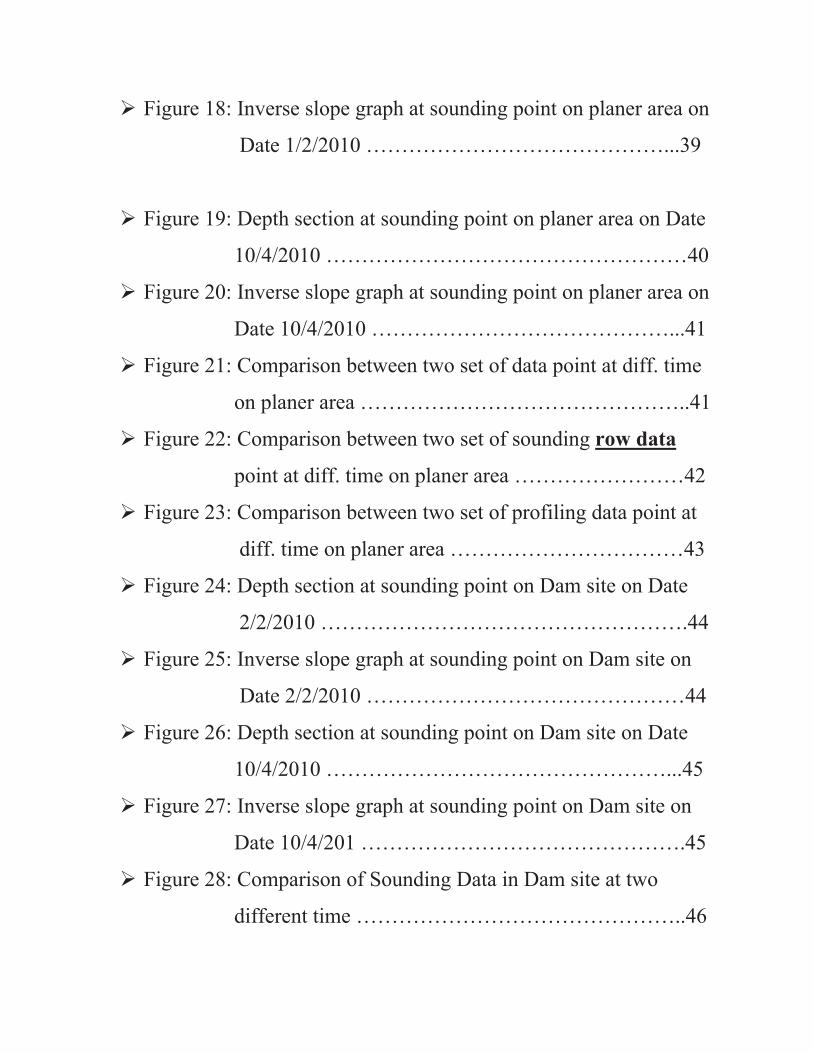
� Figure 18: Inverse slope graph at sounding point on planer area on

Date 1/2/2010 ……………………………………...39

� Figure 19: Depth section at sounding point on planer area on Date

10/4/2010 ……………………………………………40

� Figure 20: Inverse slope graph at sounding point on planer area on

Date 10/4/2010 ……………………………………...41

� Figure 21: Comparison between two set of data point at diff. time

on planer area ………………………………………..41

� Figure 22: Comparison between two set of sounding row data

point at diff. time on planer area ……………………42

� Figure 23: Comparison between two set of profiling data point at

diff. time on planer area ……………………………43

� Figure 24: Depth section at sounding point on Dam site on Date

2/2/2010 …………………………………………….44

� Figure 25: Inverse slope graph at sounding point on Dam site on

Date 2/2/2010 ………………………………………44

� Figure 26: Depth section at sounding point on Dam site on Date

10/4/2010 …………………………………………...45

� Figure 27: Inverse slope graph at sounding point on Dam site on

Date 10/4/201 ……………………………………….45

� Figure 28: Comparison of Sounding Data in Dam site at two

different time ………………………………………..46

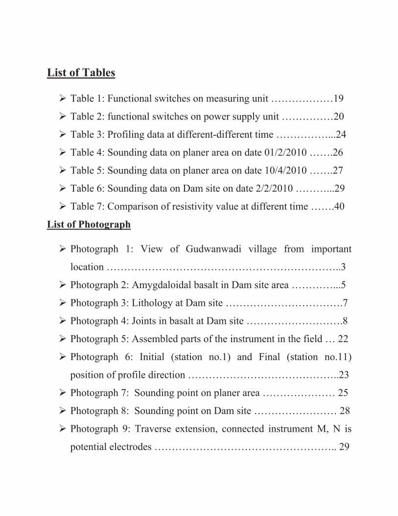
List of Tables

� Table 1: Functional switches on measuring unit ………………19

� Table 2: functional switches on power supply unit ……………20

� Table 3: Profiling data at different-different time ……………...24

� Table 4: Sounding data on planer area on date 01/2/2010 …….26

� Table 5: Sounding data on planer area on date 10/4/2010 …….27

� Table 6: Sounding data on Dam site on date 2/2/2010 ………...29

� Table 7: Comparison of resistivity value at different time …….40

List of Photograph

� Photograph 1: View of Gudwanwadi village from important

location …………………………………………………………..3

� Photograph 2: Amygdaloidal basalt in Dam site area …………...5

� Photograph 3: Lithology at Dam site …………………………….7

� Photograph 4: Joints in basalt at Dam site ……………………….8

� Photograph 5: Assembled parts of the instrument in the field … 22

� Photograph 6: Initial (station no.1) and Final (station no.11)

position of profile direction ……………………………………..23

� Photograph 7: Sounding point on planer area ………………… 25

� Photograph 8: Sounding point on Dam site …………………… 28

� Photograph 9: Traverse extension, connected instrument M, N is

potential electrodes …………………………………………….. 29

1

Chapter 1: Introduction

1.1Objective:

Site characterization and geophysical studies using electrical resistivity technique In

Gudwanwadi Dam Site, Karjat Maharashtra.

1.2Introduction:

Geophysical techniques are important in deciphering the subsurface and structure. The electrical

(DC) resistivity method, one of the significant geophysical methods, is based on the

measurement of electrical property called electrical resistance, of the subsurface material. Later

apparent resistivity of the subsurface material is calculated by this resistance using formula

ρ = R*K, where K is called geometrical factor. The electrical resistance of a wire would be

expected to be greater for a longer wire, less for a wire of larger cross sectional area, and would

be expected to depend upon the material out of which the wire is made. Experimentally, the

dependence upon these properties is a straightforward one for a wide range of conditions, and the

resistance of a wire can be expressed as,

Where ρ=resistivity, L=length, A= cross-sectional area

Resistance is not the fundamental property of material through which current passes. It depends

on the geometry of the material. Resistivity is defined as the resistance in the wire, times the

cross-sectional area of the wire, and divided by the length of the wire. It is generally indicated by

the Greek symbol ρ (Rho) in units of Ω· m. Resistivity describes how easily the material can

transmit electrical current. A high value of resistivity implies that the material is easily that the

material implies that the material is very resistant to flow electric current. Low values of

resistivity imply that the material transmits electrical current very easily.

2

Fig 1: Relation between resistance and resistivity

It is an intrinsic property of a material. The resistivity of a conductor depends on its composition

and its temperature. As a characteristic property of each material, resistivity is useful in

comparing various materials on the basis of their ability to conduct electric current. As

temperature increases, the resistivity of a metallic conductor usually increases and that of

a semiconductor usually decreases. That‟s why resistivity is used to interpret the electrical

properties of the subsurface.

This method is very useful for,

Characterize subsurface hydrogeology,

Determine depth to bedrock/overburden

Determine depth to groundwater

Quantitative assessment of groundwater reserve of unconfined aquifer

Map stratigraphy

Map clay aquitards

Map saltwater intrusion

Map vertical extent of certain types of soil and groundwater contamination.

Estimate landfill thickness.

To understand the location of abandoned coal mine.

Resistance = R

Resistivity, ρ=

3

Chapter 2: Survey area:

Survey area of my field work is Gudwanwadi, Karjat Maharashtra. Gudwanwadi

(N 19 02‟27.47” E 73 23‟05.41”) area is full of fracture basalt zone. In the February month,

there is a hand pump will dry. The area is full of dense forest. People of that area are dependent

on forest. There is severe problem of water. People drink very dirty water. There is some open

hole in Dam site where water level is very near to surface, people take water from there. Flow

rate is very low. They just filter it by very ordinary filter after that they use. Due to fracture,

water blow out and it can‟t stay in the reservoir. Our plane is to detect the fracture zone or water

saturation zone, so that people can survive there easily. Electrical prospecting methods play an

important role to solve the problem.

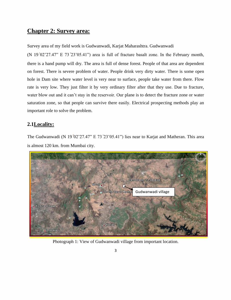
2.1Locality:

The Gudwanwadi (N 19 02‟27.47” E 73 23‟05.41”) lies near to Karjat and Matheran. This area

is almost 120 km. from Mumbai city.

Photograph 1: View of Gudwanwadi village from important location.

Gudwanwadi village

4

2.2Accessibility:

Gudwanwadi is well linked by road. We can go there by vehicle.

2.3Climate:

The climate is tropical, very humid and warm. The average daily maximum temperature is 32.9˚c

and in winter average mean minimum temperature is 16.8˚c.

2.4 General geology of the area:

The Deccan Traps are a large igneous province located on the Deccan Plateau of west-

central India (between 17–24N, 73–74E) and one of the largest volcanic features on Earth,

basically fissure type of volcanicity. They consist of multiple layers of solidified flood basalt that

together are more than 2,000 m (6,562 ft.) thick and cover an area of

500,000 km2 (193,051 sq. mi).The Deccan Traps formed between 60 and 68 million years ago, at

the end of the Cretaceous period. The bulk of the volcanic eruption occurred at the Western

Ghats (near Mumbai) some 66 million years ago. This series of eruptions may have lasted fewer

than 30,000 years in total. Although it has been suggested that the gases released in the process

may have played a role in the Cretaceous–Tertiary extinction event, which included

the extinction of the non-avian dinosaurs. The release of volcanic gases, particularly sulfur

dioxide, during the formation of the traps contributed to contemporary climate change. Data

point to an average fall in temperature of 2 °C in this period.

2.5 Chemical composition:

Within the Deccan Traps at least 95% of the lavas are Tholeiitic basalts (Tholeiitic basalt is a

type of basalt (an igneous rock) which includes very little sodium as compared with other

basalts. Chemically, this type of rock has been described as sub alkaline basalt.).Basalt is the

dark, fine-grained stuff of many lava flows and magma intrusions. Its dark minerals are rich in

5

magnesium (Mg) and iron (Fe); hence basalt is called a mafic rock. So basalt is mafic and either

extrusive or intrusive.

Deccan trap basalt flows can be divided into two major groups:

i. Compact

ii. Amygdaloidal

All compact basalt flows occur as thick extensive flows, some of them having been traced for

distance of up to 20 km. their thickness, though always considerable varies greatly and may be

up to 115 m.

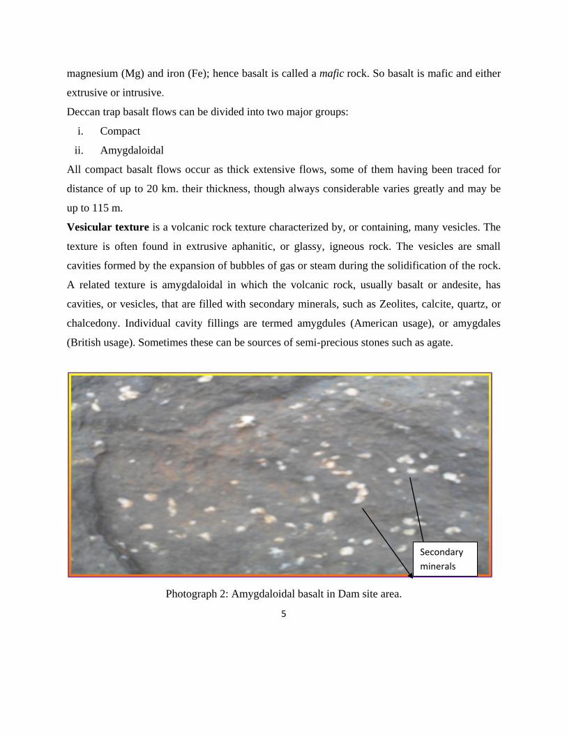
Vesicular texture is a volcanic rock texture characterized by, or containing, many vesicles. The

texture is often found in extrusive aphanitic, or glassy, igneous rock. The vesicles are small

cavities formed by the expansion of bubbles of gas or steam during the solidification of the rock.

A related texture is amygdaloidal in which the volcanic rock, usually basalt or andesite, has

cavities, or vesicles, that are filled with secondary minerals, such as Zeolites, calcite, quartz, or

chalcedony. Individual cavity fillings are termed amygdules (American usage), or amygdales

(British usage). Sometimes these can be sources of semi-precious stones such as agate.

Photograph 2: Amygdaloidal basalt in Dam site area.

Secondary

minerals

6

Amygdaloidal basalt do not occur only as upper and lower portions of thick compact basalt flows

as in normally believed, but also occur as independent flows are amygdaloidal throughout their

thickness.

2.6 Geology of the site:

1) Topographic features:

The dam site is situated at some 0.5km south of Gudwanwadi village at N 19 02‟37.2”

E 73 23‟07.4”. The valley in which the dam is proposed to be built is confined on either sides by

hills trending Northwest-Southeast, where the western hill is relatively gentler than the one on

the eastern side. The valley narrows down toward the proposed site which is ideal. The channels

upstream have a gentle slope thus a larger reservoir is obtained for the given height of the dam.

2) Drainage pattern:

The mainstream flows NW-SE as seen on the contour map. The mainstream is believed to be a

second order stream where bifurcation ratio Rb=3/1, that is, 3 primary streams join to form the

secondary stream and hence are its feeders. The three primary streams C1, C2, C3 originate in

the eastern, northwestern and northern parts of the region. Also, drainage pattern is dendrite,

therefore it can be inferred that the rock is uniform.

3) General characters and structures of rock formation and soil:

The foundation rock is Basalts which dip 1°-1.5° due east. These basalts, examined along the

stream bed, are extensively jointed, though not wide joints. A number of micro joints have also

been observed. On the valley sides, the basalts which underlie the soil cover have undergone

intensive spheroidal weathering up to a depth of 1m.The soil is lateritic, of residual nature, i.e., it

has undergone little or no transportation.

7

Photograph 3: Lithology at Dam site

In the Dam site, there is a very good exposure of lithology. On the basic of this we can expect

what will be the lithology of that area. We can see here very clear demarcation of beds.

Fig 2: Soil profile along dam alignment. (Positions Pit1 and Pit6 coincide with the

Yellow Stone Marking on field: taken from CTARA web site)

4) Lithology: The rock type here remains uniform. The region is made up of basalts which are fine-grained

equigranular. Due to this texture of basalts, water seepage capacity is low. Therefore it proves

Laterite

Spheroidal weathering

Fractured Basalt

8

good. However, presence of joints can modify the engineering properties of the rocks to some

extent.

5) Attitude of beds:

The resultant forces, namely, the weight of the dam and thrust of impounded water will be

inclined downstream. Horizontal layers offer resistance to these resultant forces. At

Gudwanwadi, the basalts are more or less horizontal with dips 1° to 1.5° due east.

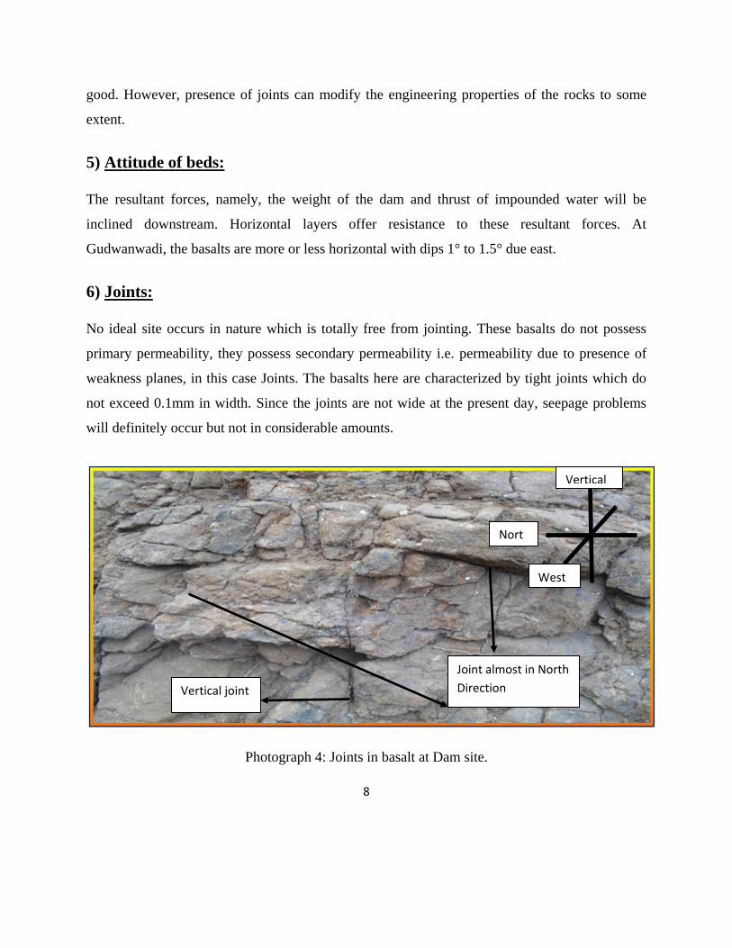
6) Joints:

No ideal site occurs in nature which is totally free from jointing. These basalts do not possess

primary permeability, they possess secondary permeability i.e. permeability due to presence of

weakness planes, in this case Joints. The basalts here are characterized by tight joints which do

not exceed 0.1mm in width. Since the joints are not wide at the present day, seepage problems

will definitely occur but not in considerable amounts.

Photograph 4: Joints in basalt at Dam site.

Vertical

Nort

h

West

Vertical joint

Joint almost in North

Direction

9

But these joints may eventually widen and hence precautions must be taken (check Corrective

and Precautionary measures). Also, the joints are either vertical or dip steeply towards the north,

hence direct loss of water downstream through joints will not occur considerably. In fact it may

make easy to recharge.

7) Groundwater conditions:

One of the most important things near Gudwanwadi village there is a hand pump whose depth is

about 96 feet, means around 29.2 meter. This is one of evidence of Groundwater level. The

groundwater will however tend to fluctuate on a monthly and yearly basis. The general water

table (encountered at 99m contour height) is more or less above the top water level of the

proposed reservoir. This is a favorable situation, as there will be less risk of much water loss

from the reservoir. This suggests that the underlying foundation basalts are of massive and

impervious nature. We can say that the massive basalts are of a previous lava flow while the

jointed and spheroidal weathered basalts are of recent episodes of eruption. An alternative

hypothesis can be that the underlying basalts are also jointed up to a certain depth and

oversaturated with water because of which water was encountered. This will be ascertained only

after excavation. Either way, extent of seepage will remain more or less same.

10

Chapter 3: Theory and Principle of Electrical Resistivity Method

The electrical resistivity method is an active geophysical method. It employs an artificial source

which is introduced into the ground though a pair of electrodes. The procedure involves

measurement of potential difference between other two electrodes in the vicinity of current flow.

Apparent resistivity is calculated by using the potential difference for the interpretation. The

electrodes by which current is introduced into the ground are called Current electrodes and

electrodes between which the potential difference is measured are called Potential electrodes.

Fig 3: A, B are current electrodes and M, N are potential electrodes.

Potential at M,

=

Potential at N,

=

11

Potential difference between M and N,

=

}

Basically we use direct currents but we can also use low frequency alternating currents to

investigate the electrical properties (resistivity) of the subsurface.

In all of these arrays, current is injected into the ground using two electrodes (from A and B) and

the resulting voltage is measured using the remaining two electrodes (from M and N). The

electrode arrays are used for different types of resistivity surveys.

3.1 Some Advantage and Disadvantages of the arrays:

3.1.1 Wenner array:

Wenner array is relatively sensitive to vertical changes in the subsurface resistivity below

the center of the array.

It is less sensitive to horizontal changes in the subsurface resistivity.

The Wenner is good in resolving vertical changes (i.e. horizontal structures), but

relatively poor in detecting horizontal changes (i.e. narrow vertical structures).

Compared to the other arrays, the Wenner array has a moderate depth of investigation.

The geometrical factor for Wenner array, which is 2*PI*a, is smaller than the geometrical

factor for other array.

Among the common arrays, the Wenner array has the strongest signal strength. This can

be an important factor if the survey is carried in areas with high background noise.

All electrodes must be moved for each reading

Required more field time

More sensitive to local and near surface lateral variations

12

3.1.2 Schlumberger array:

Effect of lateral variations in resistivity are recognized and corrected more easily on

Schlumberger than Wenner. Less sensitive to lateral variations in resistivity.

Slightly faster in field operation.

Small corrections to the field data.

Interpretations are limited to simple, horizontally layered structures.

For large current electrodes spacing, very sensitive voltmeters are required.

3.1.3Dipole-Dipole array:

This array is most sensitive to resistivity to resistivity changes between the electrodes in

each dipole pair.

Thus the dipole-dipole array is very sensitive to horizontal changes in resistivity, but

relatively insensitive to vertical changes in the resistivity.

One possible disadvantage of the array is the very small signal strength for large values

of the “n” factor. The voltage is inversely proportional to the cube of the “n” factor.

If more signal (voltage) is needed than can be provided with the Dipole-dipole array, the

Pole-dipole array can be used.

3.1.4 Pole –Pole array:

In practice the ideal pole-pole array, with only on current and one potential electrode,

does not exist.

Penetration depth is very high.

Signal strength is low.

The disadvantage of this array is that because of the large distance between the P1 and P2

electrodes, it is can pick up a large amount of telluric noise which can severely degrade

the quality of the measurement. Thus this array is mainly used in survey where relatively

small electrode spacing (<10 m) are used.

13

Figure 4: Different-Different combination of four electrode system

There are two techniques for doing electrical (DC) resistivity survey:

i. Profiling

ii. Sounding

3.2 Profiling:

In this case the spacing between the electrodes remains fixed, depth of investigation, but the

entire array is moved along a straight line. This gives the information about lateral changes in the

subsurface resistivity. It cannot detect vertical changes in the resistivity. Interpretation of the data

from profiling survey is mainly qualitative. Resistivity profiling is used to map changes in the

bedrock and overburden resistivity. If the overburden resistivity does not change laterally, the

method can be used to map variations in the elevation of the bedrock surface. Resistivity

profiling are often done using only one electrode spacing and, therefore, do not provide the

variation of resistivity with depth.

14

3.3 Sounding:

In this technique electrode spacing is not remain fixed. This technique gives the vertical changes

in the resistivity. Lateral changes in the subsurface resistivity will cause changes in the apparent

resistivity values that might be and frequently are misinterpreted as the changes with depth in the

subsurface resistivity. The depth of investigation (current penetration) also depends upon the

array type and electrode spacing. Resistivity soundings provide the resistivity and depths of the

layers under the sounding site.

3.4 Detection of Weak and Fracture zone:

Geophysical methods are commonly used to find fractures in bedrock and can also be used to

find weak zones. Generally, fracture zones are likely to contain more moisture than non-

fractured bedrock, making them more electrically conductive, as well as having a lower seismic

velocity. Fracture zones may provide the following physical parameter differences compared to

the host rock:

1. Lower resistivity (higher conductivity).

2. Bedrock topographic depressions due to fracturing and weathering.

The resistivity method can be used to locate fracture zones and weak zones if they have a

resistivity contrast with the host rocks. Fractures in bedrock occur most often in competent rocks

that are not able to adjust to the stresses placed upon them. Shale and clay are less likely to be

fractured than harder rocks such as limestone and metamorphic rocks. Limestone may also

develop solution cavities and fissures in addition to fractures. Since geophysical methods will

rarely be able to detect individual fractures unless they are very large, regions of fracturing,

called fracture zones, are more likely to provide geophysical targets. Weak zones are regions or

zones where the bedrock cannot tolerate significant compressive stress without deformation.

They often have physical properties similar to those of fracture zones but may be more extensive.

Weak zones may occur if the bedrock surface is a series of dipping layers with some layers being

less competent than other layers. This may occur if one of the dipping layers is more prone to

15

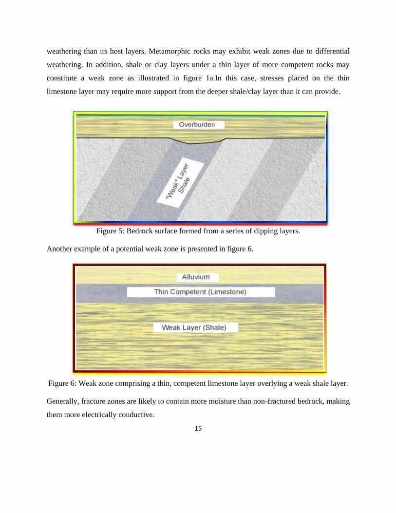
weathering than its host layers. Metamorphic rocks may exhibit weak zones due to differential

weathering. In addition, shale or clay layers under a thin layer of more competent rocks may

constitute a weak zone as illustrated in figure 1a.In this case, stresses placed on the thin

limestone layer may require more support from the deeper shale/clay layer than it can provide.

Figure 5: Bedrock surface formed from a series of dipping layers.

Another example of a potential weak zone is presented in figure 6.

Figure 6: Weak zone comprising a thin, competent limestone layer overlying a weak shale layer.

Generally, fracture zones are likely to contain more moisture than non-fractured bedrock, making

them more electrically conductive.

16

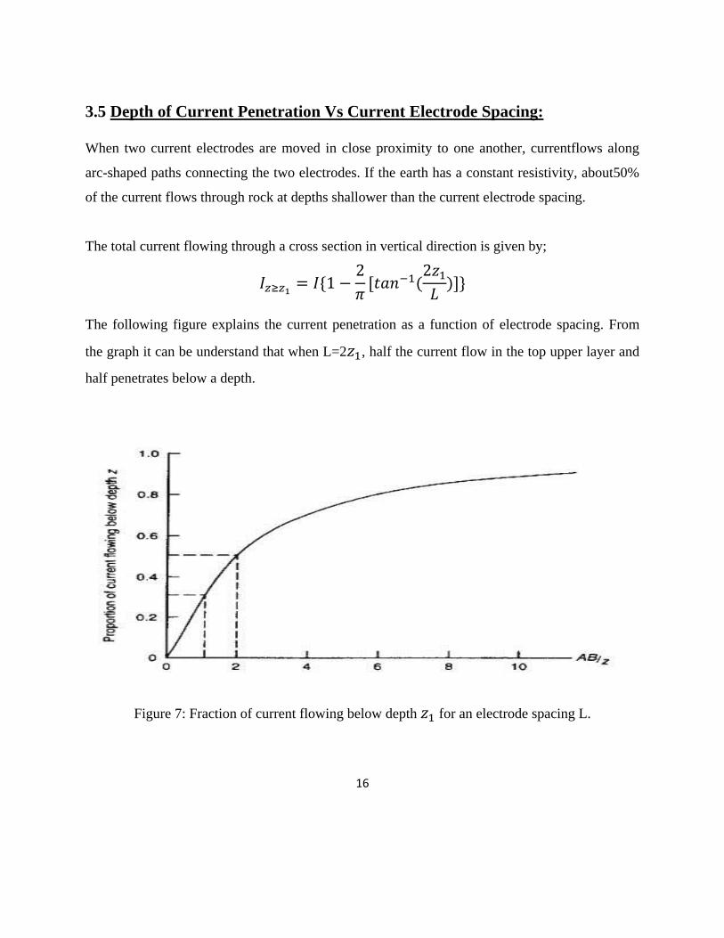
3.5 Depth of Current Penetration Vs Current Electrode Spacing:

When two current electrodes are moved in close proximity to one another, currentflows along

arc-shaped paths connecting the two electrodes. If the earth has a constant resistivity, about50%

of the current flows through rock at depths shallower than the current electrode spacing.

The total current flowing through a cross section in vertical direction is given by;

The following figure explains the current penetration as a function of electrode spacing. From

the graph it can be understand that when L=2 , half the current flow in the top upper layer and

half penetrates below a depth.

Figure 7: Fraction of current flowing below depth for an electrode spacing L.

17

What this implies is that by increasing the electrode spacing, more of the injected current will

flow to greater depths, as indicated in the figure 8. Because the total resistance in the electrical

path increases as electrode spacing is increased, to get current to flow over these longer paths

requires a larger generator of electrical current. Thus, the maximum distance that current

electrodes can be separated by is in part dictated by the size of the generator used to produce the

current.

Figure 8: Comparison of penetration depth with electrode spacing.

Assuming for a moment that we have a large enough generators to produce a measurable current

in the ground at large current electrode spacings, this increase in the depth of current penetration

as current electrode spacing increases suggests a way in which we could hope to decipher the

resistivity structure of an area. Because current flows mostly near the Earth's surface for close

electrode spacings, measurements of apparent resistivity at these electrode spacings will be

dominated by the resistivity structure of the near surface. If the current and potential electrodes

are spread apart and the apparent resistivity remeasured, these measurements will incorporate

information on deeper Earth structure.

18

Chapter 4: Instrumentation and Survey methodology:

The resistivity meter which I used to acquire the electrical resistivity data is SSR-MP-AT

manufactured by Integrated Geo Instruments & Services Pvt. Ltd. (IGIS), Hyderabad. This

equipment is a Resistivity Imaging System and can be employed for resistivity profiling as well

as resistivity scanning of the subsurface.

In the presence of random (non-coherent) earth noises, the signal to noise ratio can be enhanced

by √N where N is the number of stacked readings. SSR-MP-AT is a microprocessor-based signal

stacking Resistivity Meter, in which running averages of measurements [1, (1+2)/2, (1+2+3)/3,

......... (1+2+....+16)/16] up to the chosen stacks are displayed and the final average is stored

automatically in memory utilizing the principle of stacking to achieve the benefit of high signal

to noise ratio.

The SSR-MP-AT is programmable through user-friendly menu for its operation and entry of

survey parameters like Survey No., Electrode Separations etc. The SSR-MP-AT Resistivity

meter directly gives the Resistance (ratio of ∆V and current) with a resolution up to 10-5 ohms at

1 A input current.

4.1 Description of the system:

The Multi-Electrode Resistivity Meter system comprises:

The main measuring unit (Resistivity Meter)

G-Unit (Power supply unit to inject current into the ground)

4 Stainless Steel electrodes

Connecting cables

4.1.1Measuring Unit (M-Unit):

A photograph of the instrument is shown below figure various controls and other functional

switches are enumerated below:

19

1. C1 & C2 Terminal for connecting current electrodes.

2. P1 & P2 Terminal for potential electrode connection.

3. Display Alphanumeric display to show the menu and measured values.

4. Power on ON-OFF Power switch

5. Measure Sets the measuring unit from standby mode to measurement mode.

6. Ref 1 Ref 1 to be connected to Ref 1 of G-Unit

7. Key pad Key pad to interact with the system and entry of spacing values, no. of stacks

8. To PC Facilitates connection to the computer for data transfer through data transfer

cable

9. Ref 2 Ref 2 to be connected to Ref 2 of G-Unit

Table 1: Functional switches on measuring unit

Figure 9: Measuring unit

4.1.2 G-Unit or Power supply unit:

A photograph of the G-Unit (Power supply) is shown below figure various controls and other

functional switches are enumerated below:

1 3

2

5

4

6 9

8

7

20

1. Bat Check Switch to check the battery level on the VU meter.

2. Fuse To protect the circuit in case of overload. If there is no display when all

connections are made, check the fuse and change it, if necessary.

3. Charge Connector to facilitate charging of the built-in battery. Connect the charger to

this 3-pin connector to charge (2 X 12V) batteries, which are housed in the

bottom compartment of the G-unit.

4. VU Meter Meter to show the condition of the battery when the bat. Check switch is

pressed.

5. Ref. 1 To be connected to Ref.1 of the Measuring Unit.

6. Ref. 2 To be connected to Ref.2 of the Measuring Unit.

Table 2: functional switches on power supply unit

Figure 10: G-unit (Power supply)

4.1.3 Principle of Measurement:

The SSR-MP-AT contains mainly two units‟ Current unit and Microprocessor-based Measuring

unit. The current unit sends bipolar signals into the ground at a frequency of about 0.5Hz. The

6

3

2

5

1

4

21

receiver has a 4½ digit dual-slope analog to digital converter (ADC) unit, which can measure the

ground potentials and current with resolution up to 100V and 100A respectively. The

microprocessor controls the current unit, determines the attenuation level for potential

measurements, computes the resistance values, averages the measured values, keeps the data in

memory, displays and transfers the data to PC.

4.1.4 Current Unit:

This unit sends bipolar current into the ground. This unit has three voltage settings 50V, 150V

and 350V, which are controlled by the microprocessor of the measuring unit. This unit is

powered by 2 x 12 V rechargeable batteries.

4.1.5 Measuring (Microprocessor) Unit:

This is the main unit, which measures the current and potential values, calculates the resistance

and apparent resistivity, stores in the memory and gives the output through the display. This unit

is to be programmed. This unit is powered by the same batteries meant for current unit.

4.2 Field Layout and Data Acquisition:

Resistivity surveys are made to satisfy the need of two distinctly different kinds of interpretation

problem:

The variation of resistivity with depth, reflecting more or less horizontal stratification of

earth material.

Lateral variation in resistivity that may indicate soil lenses, isolated ore bodies, faults, or

cavities.

For the first kind of problem, measurements of apparent resistivity are made at a single location

(or around a single center point) with systematically varying electrode spacings. This procedure

is something called vertical electrical sounding (VES), or vertical profiling. Surveys of lateral

22

variations may be made at spot or grid locations or along definite lines of traverse, a procedure

sometimes called horizontal profiling. Either the Schlumberger or, less effectively, the Wenner

array is used for sounding, since all commonly available interpretation methods and

interpretation aids for sounding are based on these two arrays. In the use of either method, the

center point of the array is kept at affixed location, while the electrode locations are varied

around it. The apparent resistivity values, and layer depths interpreted from them, are referred to

the center point.

Photograph 5: Assembled parts of the instrument in the field

After finalizing the target point for Vertical Electrical Sounding, the other parameters to be

considered are:

Depth to the investigated,

Depth resolution, and

Direction of required traverse.

After fixing of center point of the array or sounding point, drives the current electrode (A, B) and

potential electrodes (M, N) into the ground at fixed distance. Then connect these electrodes (A,

B) and (M, N) through the wire of the spools to the C1, C2 and P1, P2 inserting point in the

measuring unit respectively. The important point to note is that the electrodes are to be driven

23

deep enough to get good galvanic contact with the ground; if necessary, wetting the ground at

electrodes is recommended. Now complete the circuitry by joining the reference 1 and reference

2 of the G-Unit (Power Supply) to reference 1 and reference 2 terminals in the measuring unit

and take the measurement for this AB/2 and MN/2 combination. The measuring unit will display

the R (Resistance) and ρ (Resistivity) value on display screen. Then write down this

measurement and press Enter in M-Unit. It will automatically store in the memory. Now for

further measurement increase the AB/2 and MN/2 keeping the same. MN/2 will be increased

further when signal is too weak.

4.2.1Acquired Field Data and Field Position:

We have collected data two times at same places in different -different season.

4.2.1.1 Profiling:

We have taken our profile direction almost 19˚ from north towards west. From station no.1 we

have taken 20 meter station interval and reaches at station no.11.

Photograph 6: Initial (station no.1) and Final (station no.11) position of profile direction

Station no.1

Station no.11

24

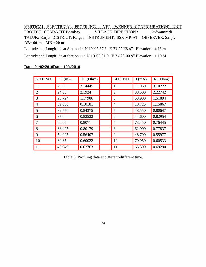
VERTICAL ELECTRICAL PROFILING - VEP (WENNER CONFIGURATION) UNIT

PROJECT: CTARA IIT Bombay VILLAGE DIRECTION : Gudwanwadi

TALUK: Karjat DISTRICT: Raigad INSTRUMENT: SSR-MP-AT OBSERVER: Sanjiv

AB= 60 m MN =20 m

Latitude and Longitude at Station 1: N 19 02‟37.3” E 73 22‟58.6” Elevation: ± 15 m

Latitude and Longitude at Station 11: N 19 02‟31.0” E 73 23‟00.9” Elevation: ± 10 M

Date: 01/02/2010Date: 10/4/2010

Table 3: Profiling data at different-different time.

SITE NO. I (mA) R (Ohm) SITE NO. I (mA) R (Ohm)

1 26.3 3.14445 1 11.950 3.10222

2 24.85 2.1924 2 38.500 2.22742

3 23.724 1.17986 3 53.900 1.51894

4 39.050 0.10181 4 18.725 1.15867

5 39.550 0.84375 5 48.550 0.80647

6 37.6 0.82522 6 44.600 0.82954

7 66.65 0.8071 7 73.450 0.76445

8 68.425 0.80179 8 62.900 0.77837

9 54.025 0.56407 9 48.700 0.55977

10 60.65 0.60022 10 70.950 0.60533

11 46.949 0.62763 11 65.500 0.69290

25

4.2.1.2 Sounding:

4.2.1.2.1 Sounding at the planer area:

We have taken our sounding point almost at the center of profile line.

Photograph 7: Sounding point on planer area

Sounding point

Dam

26

VERTICAL ELECTRICAL SOUNDING –VES (SCHLUMBERGER CONFIGURATION)

PROJECT: CTARA IIT Bombay VILLAGE DIRECTION: Gudwanwadi

TALUK: Karjat DISTRICT: Raigad INSTRUMENT: SSR-MP-AT

OBSERVER: Sanjiv

DATE: 1/02/2010 Latitude and Longitude: N 19 02‟35.1” E 73 23‟00.0” Elevation: ± 16 m

S.No. AB/2 (m) MN/2 (m) I(mA) R(Ohm) ρa(Ohm-m)

1 1.5 0.5 14.3 41.527 260.906

2 2 0.5 14.7 18.3682 216.382

3 2.5 0.5 13.35 9.66807 182.227

4 3 0.5 28.35 5.6427 155.102

5 4 0.5 16.6 2.95955 146.43

6 5 0.5 20.199 1.60488 124.779

7 6 0.5 23.6 0.97432 109.421

8 6 1 23.95 2.17297 119.457

9 8 1 28.95 0.98198 97.1716

10 10 1 24.05 0.54215 84.3053

11 15 1 19.3 0.21561 75.8601

12 15 2 19.575 0.43663 75.7842

13 20 2 26.75 0.28014 87.126

14 25 2 19.5 0.21407 104.406

15 30 2 18.9 0.17335 121.988

16 30 6 19.05 0.52663 119.114

17 40 6 31.774 0.2821 115.502

18 50 6 34 0.23681 152.756

19 60 6 47.7 0.2027 189.125

20 60 10 47 0.33791 185.767

21 70 10 44.2 0.22076 166.446

22 80 10 51.975 0.15483 153.215

23 90 10 40.45 0.12664 159.13

24 100 10 62.8 0.10145 157.767

Table 4: Sounding data on planer area on date 01/2/2010.

27

Date: 10/04/2010

Latitude and Longitude: N 19 02‟35.1” E 73 23‟00.0” Elevation: ± 16 M

S.No. AB/2 (m) MN/2(m) I (mA) R(Ohm) ρa(Ohm-m)

1 1.5 0.5 24.35 37.3991 234.971

2 2 0.5 38.3 18.2219 214.659

3 2.5 0.5 36.2 10.5784 199.386

4 3 0.5 22.0 6.61079 181.712

5 4 0.5 26.100 2.98761 147.821

6 5 0.5 30.399 1.73959 135.252

7 6 0.5 9.0909 1.11046 124.71

8 6 1 9.6999 2.35167 129.282

9 8 1 35.554 0.98532 97.5017

10 10 1 31.9 0.53439 83.0983

11 15 1 23.1 0.21579 75.9236

12 15 2 23.25 0.42118 73.102

13 20 2 13.85 0.28809 89.5984

14 25 2 23.357 0.21934 106.973

15 30 2 22.15 0.16093 113.242

16 30 6 22.25 0.51600 116.709

17 40 6 18.975 0.36112 147.855

18 50 6 19.55 0.26953 173.857

s19 60 6 49.050 0.19926 185.913

20 60 10 49.150 0.33787 185.747

21 70 10 36.350 0.24047 181.301

22 80 10 42.575 0.16682 165.077

23 90 10 39.600 0.12849 161.458

24 100 10 54.949 0.10418 162.01

Table 5: Sounding data on planer area on date 10/4/2010.

28

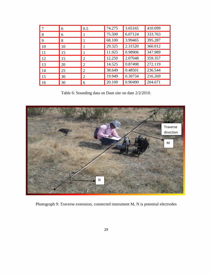
4.2.1.2.2 Sounding at Dam site:

Date: 2/02/2010

Latitude and Longitude: N 19 02‟37.2” E 73 23‟07.4” Elevation: ± 10 m

Photograph 8: Sounding point on Dam site

Date: 2/2/2010

S.No.

AB/2 (m) MN/2 (m)

I (mA)

R (Ohm)

ρa (Ohm-m)

1 1.5 0.5 133.92 34.5178 216.868

2 2 0.5 125.65 22.1094 260.454

3 2.5 0.5 113.75 15.2763 287.933

4 3 0.5 89.90 11.8557 325.881

5 4 0.5 119.89 7.26879 359.638

6 5 0.5 43.85 4.81773 374.577

Sounding point

Dam

Gudwanwadi village

29

7 6 0.5 74.275 3.65165 410.099

8 6 1 75.500 6.07124 333.763

9 8 1 68.100 3.99465 395.287

10 10 1 29.325 2.31520 360.012

11 15 1 11.925 0.98906 347.989

12 15 2 12.250 2.07048 359.357

13 20 2 14.525 0.87498 272.119

14 25 2 38.649 0.48501 236.544

15 30 2 19.949 0.30734 216.269

16 30 6 20.100 0.90490 204.671

Table 6: Sounding data on Dam site on date 2/2/2010.

Photograph 9: Traverse extension, connected instrument M, N is potential electrodes

Traverse

direction

M

N

30

Chapter 5: Interpretation Theory:

The interpretation problem for resistivity data is to use the curve of apparent resistivity versus

electrode spacing, plotted from field measurement, to obtain the parameters of the geoelectrical

section: the layer resistivities and thickness.

5.1 Conventional approach of Data Processing:

Conventionally the plot between apparent resistivity and electrode separation (a) in case of

Wenner configuration and between apparent resistivity and half current electrode separation

(AB/2), in case of Schlumberger configuration on double logarithmic scale is used for analysis of

thicknesses and resistivities of the subsurface layers. The data density is between 6-8 per log

cycle of electrode separation. Even if the data density is higher than that it would not give any

additional advantage because of logarithmic plotting.

There are various techniques for interpretation. For qualitative interpretation H, Q, A, K type

curve technique is used and for quantitative interpretation Master curves matching technique,

Inversion technique and Inverse slope technique can be used.

5.2 Master curve technique:

One of a set of theoretical curves, calculated for known models, against which a field curve can

be matched. If the two fit very closely the model is considered to apply reasonably well to the

field situation and the curve is known as the master curve. Master curves were used extensively

in electrical resistivity depth sounding, but are being replaced by micro-computer curve

matching which is much more accurate and more sensitive to real-life situations.

To fit the field curve in the given master curve, we have to shift the x and y-axis of field curve to

get a perfect fitting. After getting perfect fit, we determine the layer parameter.

31

5.3 Interpretation using two-layer master curve:

By using following procedure we will get the thickness and resistivity of the subsurface.

I. First plot vs.

on log-log transparent sheet of the same modulus of the master

curve.

II. Now superimpose field curve on the two layer master curve and shift field curve in x-axis

and y-direction to get perfect fit.

III. In the best fit position mark the origin of master curve (1, 1) on the transparent field

curve

The value of origin on field curve gives the value of ( . Once we know the and , the

ratio

is known we can compute Thus we have determine , , and . We interpret 3-

layer cases in similar way.

Figure 11: Two layer master curves

32

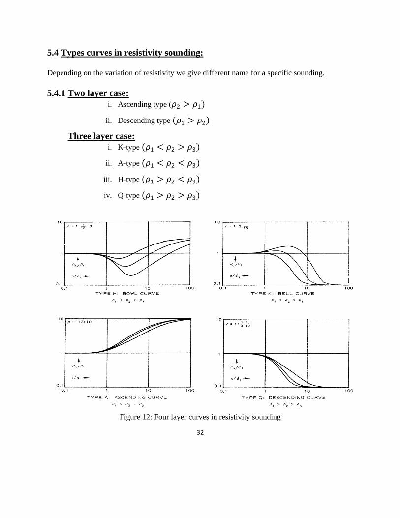
5.4 Types curves in resistivity sounding:

Depending on the variation of resistivity we give different name for a specific sounding.

5.4.1 Two layer case:

i. Ascending type (

ii. Descending type

Three layer case:

i. K-type

ii. A-type

iii. H-type

iv. Q-type

Figure 12: Four layer curves in resistivity sounding

33

Four layer case:

i. KH-type

ii. KQ-type

iii. AA-type

iv. AK-type

v. HA-type

vi. HK-type

vii. QH-type

viii. QQ-type

Similarly for 5 layer case 16-different types of sounding curves will be possible.

6 layer ---32 curves

7 layer ---64 curves

HH and KK type curves can‟t be drawn.

5.5 Inversion Technique:

A good inversion method must simultaneously minimize the effects of data error and model

parameter errors. The necessary requirements for inversion of any geophysical data are a fast

forward algorithm for calculating theoretical data for initial model parameters, and a technique

for calculating derivatives of the data with respect to the model parameters. Unfortunately the

second requirement is not readily available for two-dimensional (2D) or three-dimensional (3D)

inverse resistivity problems.

There are two types of modeling:

Forward modeling with layer thickness and resistivity provided by user.

Inversion methods where models parameters iteratively estimated from data subject to user

supplied constraints.

34

However, the resistivity sounding technique (in the present form) has the following inherent

disadvantages:

The resolving power of this method is poor and is particularly true for deeper boundaries.

Due to the principle of suppression, a middle layer with resistivity intermediate between

enclosing beds will have practically no influence on the resistivity curve as long as its

thickness is small in comparison to its depth. Hence the layers with small thickness

cannot be recognized.

Due to principle of equivalence (i) a conductive layer sandwiched between two layers of

higher resistivities will have the same influence on the curve as long as the ratio of its

thickness to resistivity (h/p) remains the same and similarly (ii) a resistive layer

sandwiched between two conducting layers will have the same influence on the curve as

long as the product of its resistivity and thickness. Hence the thicknesses and resistivities

of sandwiched layers of small thickness cannot be determined uniquely.

This can be clearly demonstrated and understood from the following example. The field

sounding data was obtained with Wenner configuration and interpreted with conventional

approach – first by Curve Matching and subsequently the interpretation model is refined by

Inversion technique. You can see that the same data set can be interpreted for any model.

Figure 13: From same data set making 2 layer and 3 layer model.

35

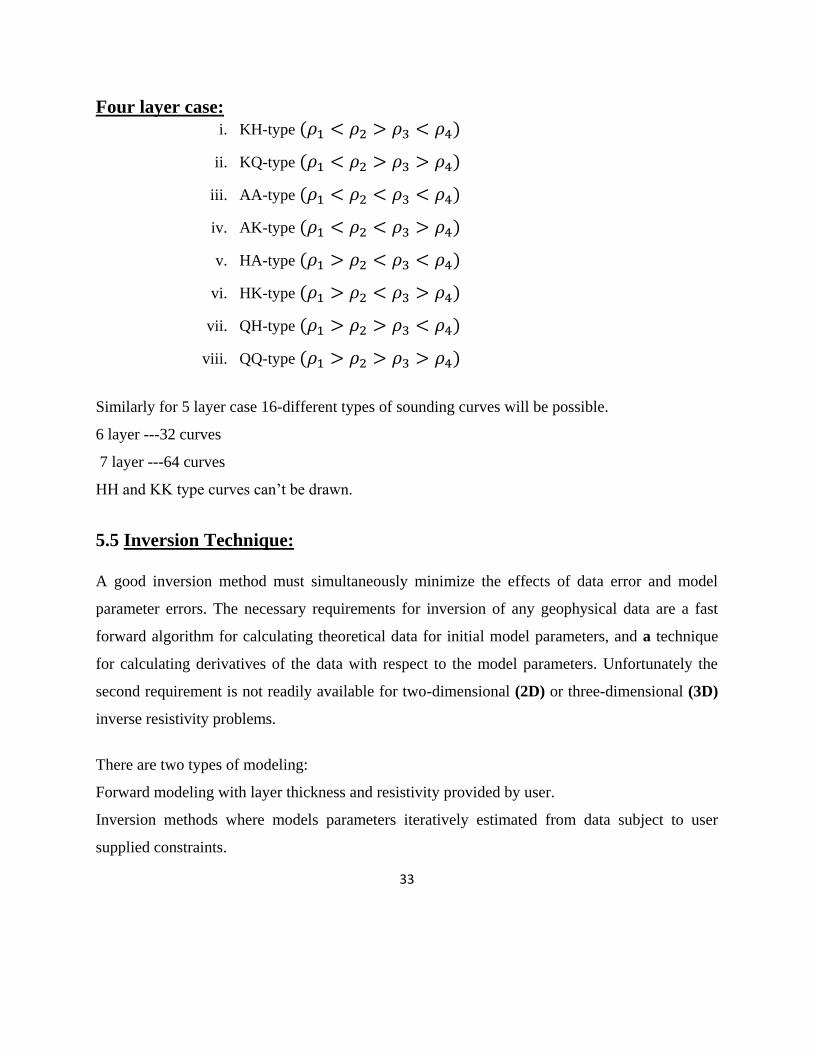
Added to this disadvantage of ambiguity in interpretation by established conventional approach

by Curve matching and inversion techniques, the resolution of the conventional approach is poor

and thin layers buried at depths more than 5-times their thickness can‟t be identified because of

the logarithmic plotting. This can be easily visualized by the following illustration.

Figure 14: Comparison of linear scale with logarithmic scale in depth.

Imagine 3 aquifers of each 10 meters thickness existing between depths 10-20, 50-60 and 90-100

m. When they are represented on a linear scale they look real and when the same aquifers are

represented on a logarithmic scale, they look very thin and the third layer between 90-100 m

depths simply looks like an interface. In such conditions, it is difficult to identify the last two

layers if the data is plotted on a logarithmic scale. This suggests that linear plotting of the data

and analyzing will be able to decipher thin layers even if they are buried at great depths,

provided the data density is adequate enough to get the signals from the target layers.

36

5.6 Inverse Slope Method:

Taking lead from this concept, Dr. KRR Chary of IGIS has invented an innovative approach to

interpret the vertical electrical sounding data with Wenner configuration. According to this

approach, the inverse of resistance measured (1/R) is plotted against the Wenner electrode

separation „a’ on a linear graph. The plotted data points and align themselves on discrete line

segments and are joined by straight lines. Each line segment represents a layer and the

intersections of the line segments correspond to the depths to the particular layers. The resistivity

of the layers is obtained by the inverse slope of the particular line segment multiplied with „2π‟.

A schematic example of the Inverse Slope method of interpretation of resistivity sounding data is

given below:

Figure 15: Plotting 1/R Vs. a (a= electrode separation)

Slope of line segment = Δy/Δx = (1/R) / a

Inverse Slope = a / (1/R) = a * R

Resistivity of the layer = „2π‟ * (Inverse Slope) = 2π * (a * R) = 2π a R

A small improvement of this is to plot (a / ρa) on the Y-axis instead of (1 / R). Then the Inverse

Slope directly gives the resistivity of the layer (No need to multiply the inverse slope with „2π‟).

37

Figure 16: Plotting (AB/2)/ρa Vs. AB/2 (AB/2= electrode separation)

Originally, the Inverse Slope method was proposed for interpretation of Wenner sounding data.

However, this method can also be used for Schlumberger data with a minor modification. For

Schlumberger sounding the linear plot has to be prepared between (AB/2) on X-axis and

{(AB/2)/ρa} on Y-axis. You should not use (1/R) for plotting since R depends on both AB/2 and

MN/2. While the inverse slope of the line segments directly gives the true resistivity of the

layers, the intersections of the line segments have to be multiplied with (2/3) to get the depths to

the interfaces. The procedure of interpretation for both these soundings is described in the

following tabular form.

5.7 Data interpretation:

I used the inverse slope interpretation technique for interpretation of the resistivity data. There is

a software provided by IGIS along with the resistivity information and the linear plot has to be

prepared between (AB/2) on X-axis and (AB/2)/ Y-axis. Now this plot gives the thickness and

resistivity of different geoelectric layers within the subsurface. Now by the geological

knowledge of subsurface we can estimates about the lithology and conductive zones in

subsurface.

38

5.7.1 Sounding point at planer area (N 19 02’35.1” E 73 23’00.0”):

For the sounding point latitude and longitude (N 19 02‟35.1” E 73 23‟00.0”) the traverse was

taken along almost N 19˚ W and the total extension of the traverse was 200m, 100m on both

side of sounding point. After plotting in software provided with instrument and making the

layered model on the basis of data quality and prior geological information, this software gives

the resistivity and thickness of each layer.

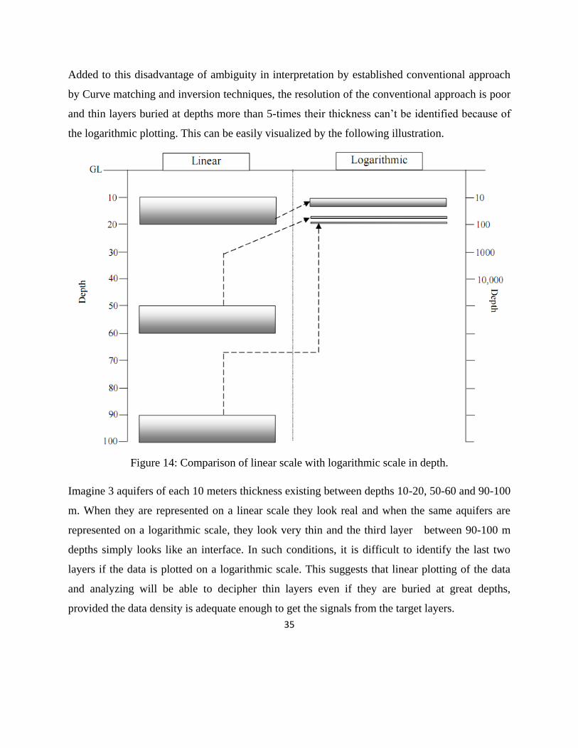
With the resistivity data only, we can‟t interpret about the exact lithology but up

to some extent. We can expect the lithology in the subsurface.

So here beneath the sounding point the top layer is Laterite with very fine loose material which is

up to depth of 10.8 meter and resistivity is about 71 Ohm-m. Below this, Laterite is again present

with very big spheroidal boulders whose resistivity is 291 Ohm-m with thickness 11.3 meter.

Below this, highly fractured basalt is present whose resistivity is 415 Ohm-m and thickness is 19

meter. Below this highly fractured basalt there is a conductive zone whose resistivity is 98 Ohm-

m and it start from depth of 41.1 meter and end with depth of 52.7 meter with thickness of 11.6

meter. This zone might be saturated with fresh water and more porous than the overlying layer.

From onwards 52.7 meter resistivity increases, resistivity in this zone is 173 Ohm-m.

This may be due to compact basalt. According to the H, K, A, Q notation of interpretation this

subsurface is showing AKH type five layer model.

39

Figure 17: Depth section at sounding point on planer area on Date 1/2/2010

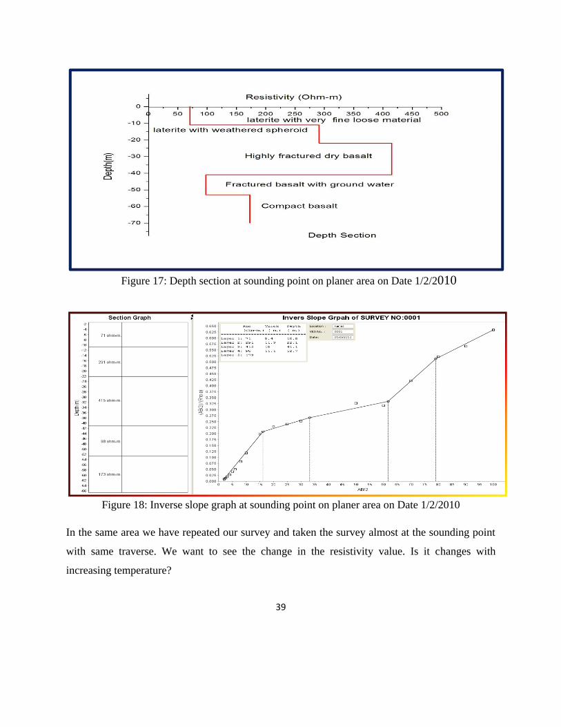
Figure 18: Inverse slope graph at sounding point on planer area on Date 1/2/2010

In the same area we have repeated our survey and taken the survey almost at the sounding point

with same traverse. We want to see the change in the resistivity value. Is it changes with

increasing temperature?

40

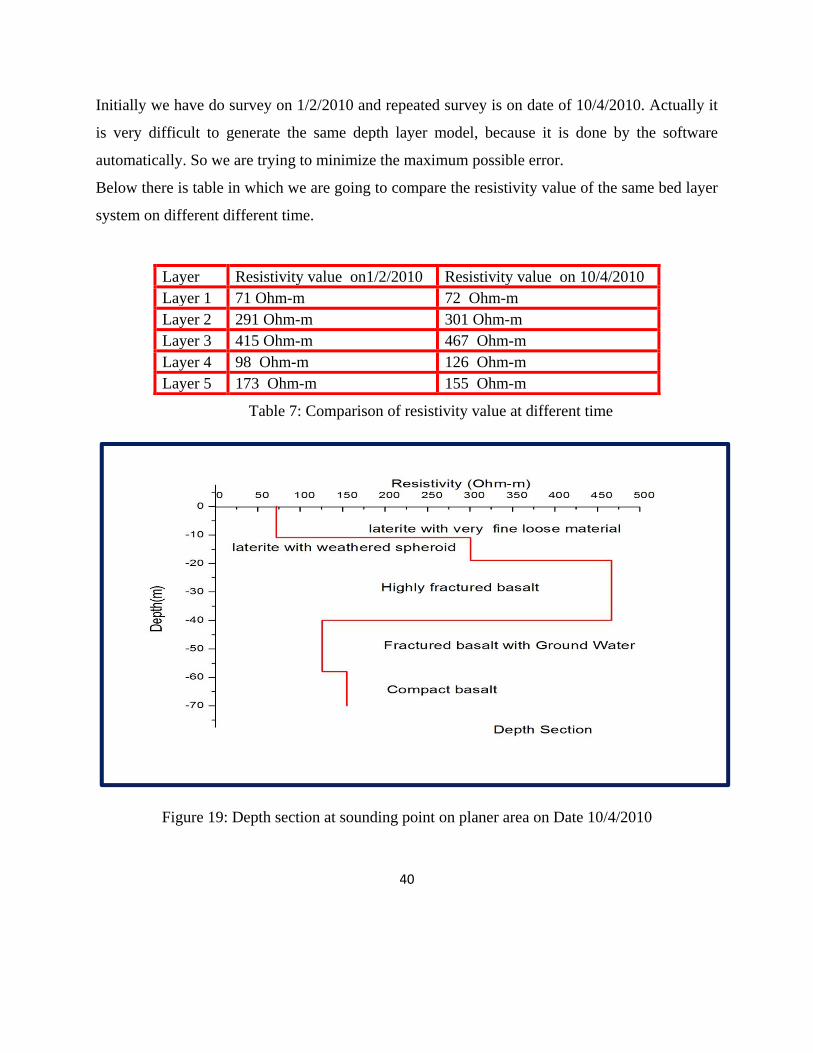
Initially we have do survey on 1/2/2010 and repeated survey is on date of 10/4/2010. Actually it

is very difficult to generate the same depth layer model, because it is done by the software

automatically. So we are trying to minimize the maximum possible error.

Below there is table in which we are going to compare the resistivity value of the same bed layer

system on different different time.

Table 7: Comparison of resistivity value at different time

Figure 19: Depth section at sounding point on planer area on Date 10/4/2010

Layer Resistivity value on1/2/2010 Resistivity value on 10/4/2010

Layer 1 71 Ohm-m 72 Ohm-m

Layer 2 291 Ohm-m 301 Ohm-m

Layer 3 415 Ohm-m 467 Ohm-m

Layer 4 98 Ohm-m 126 Ohm-m

Layer 5 173 Ohm-m 155 Ohm-m

41

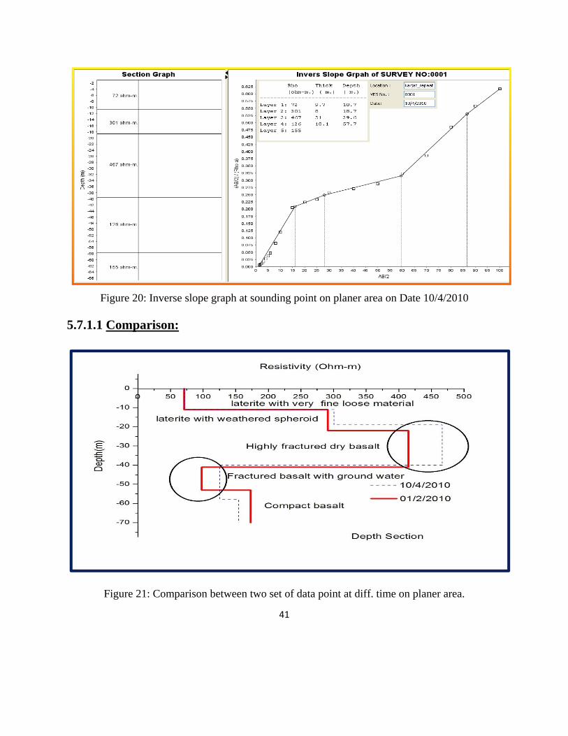
Figure 20: Inverse slope graph at sounding point on planer area on Date 10/4/2010

5.7.1.1 Comparison:

Figure 21: Comparison between two set of data point at diff. time on planer area.

42

We can easily identify the layer where resistivity increases. Layer no. 3 has resistivity increases;

it is a zone which is highly fractured. We can say that the moisture which was present at

1/2/2010 is evaporated. And layer no. 4 has resistivity also increase on 10/4/2010. Same,

evaporation have taken place. Increment is not very big but it is significant. Deviation in depth

for layer is due to software, and we have no control on this, but here we are trying to minimize

error presenting the optimal model. Actually it is a forward modeling, so it has some limitation.

Below we are presenting a graph which is formed by row data. It shows some important things.

The rectangular area shows how the resistivity is deviated from initial one. This means that at

this depth zone there is some conductive body whose resistivity increases with temperature, this

means that there may be a possibility of water saturated reservoir.

.Figure 22: Comparison between two set of sounding row data point at diff. time on planer area

43

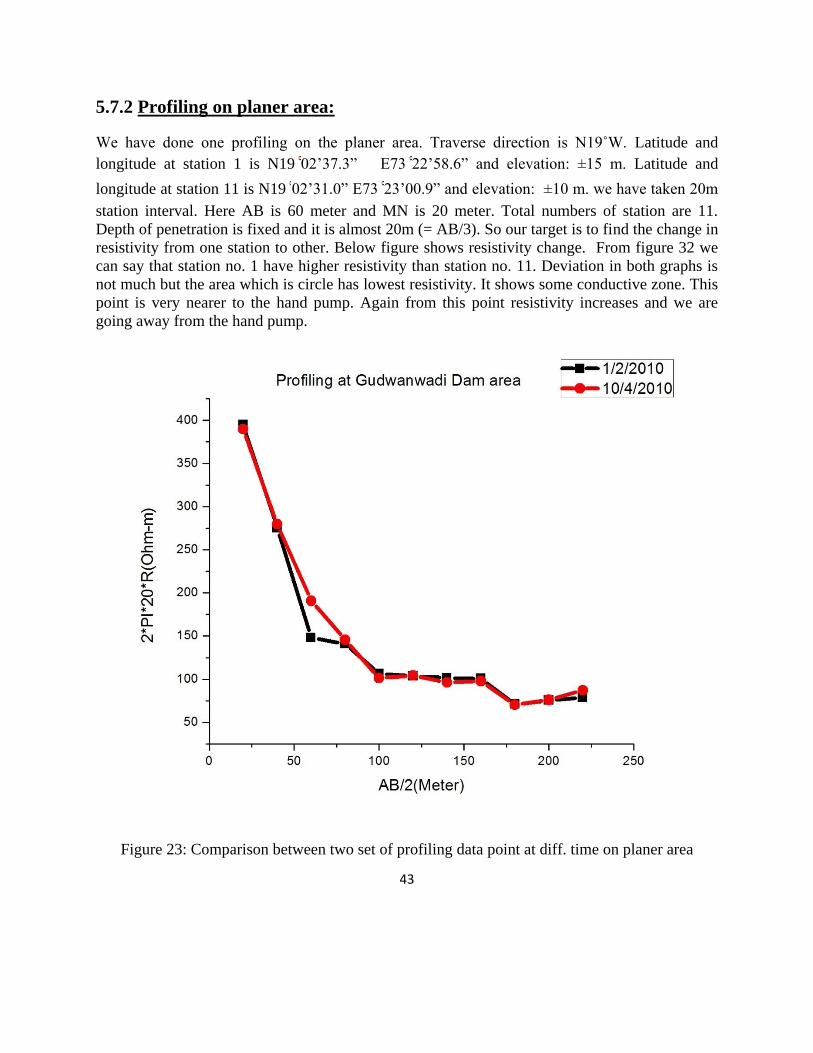
5.7.2 Profiling on planer area:

We have done one profiling on the planer area. Traverse direction is N19˚W. Latitude and

longitude at station 1 is N19 02‟37.3” E73 22‟58.6” and elevation: ±15 m. Latitude and

longitude at station 11 is N19 02‟31.0” E73 23‟00.9” and elevation: ±10 m. we have taken 20m

station interval. Here AB is 60 meter and MN is 20 meter. Total numbers of station are 11.

Depth of penetration is fixed and it is almost 20m (= AB/3). So our target is to find the change in

resistivity from one station to other. Below figure shows resistivity change. From figure 32 we

can say that station no. 1 have higher resistivity than station no. 11. Deviation in both graphs is

not much but the area which is circle has lowest resistivity. It shows some conductive zone. This

point is very nearer to the hand pump. Again from this point resistivity increases and we are

going away from the hand pump.

Figure 23: Comparison between two set of profiling data point at diff. time on planer area

44

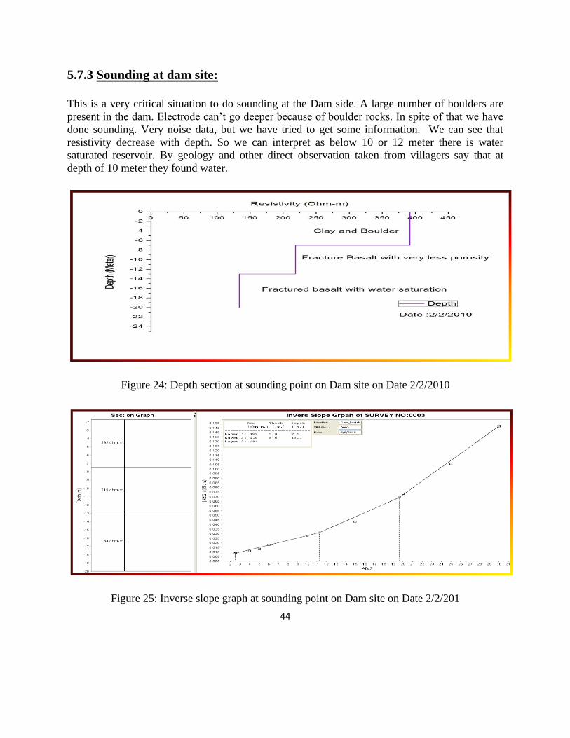
5.7.3 Sounding at dam site:

This is a very critical situation to do sounding at the Dam side. A large number of boulders are

present in the dam. Electrode can‟t go deeper because of boulder rocks. In spite of that we have

done sounding. Very noise data, but we have tried to get some information. We can see that

resistivity decrease with depth. So we can interpret as below 10 or 12 meter there is water

saturated reservoir. By geology and other direct observation taken from villagers say that at

depth of 10 meter they found water.

Figure 24: Depth section at sounding point on Dam site on Date 2/2/2010

Figure 25: Inverse slope graph at sounding point on Dam site on Date 2/2/201

45

Figure 26: Depth section at sounding point on Dam site on Date 10/4/2010

Figure 27: Inverse slope graph at sounding point on Dam site on Date 10/4/201

We can see here at depth of 12 meter on 2/2/2010 has higher resistivity than 10/4/2010. But in

above case the resistivity is increases. It should be increase bust it is decreases.

46

Comparison:

Figure 28: Comparison of Sounding Data in Dam site at two different time

It is because of a lot of boulders in dam site; on 10/4/2010 it might be possible the electrodes

have penetrated very well so reading is better than previous one. But the final result is that at 12

meter there is water.

5.8 Conclusion:

One of my batch mats also done resistivity survey in the same area. He has taken profile

direction across to my profile direction in the planer area. His interpretation is like that,

resistivity increases with depth. It is very confusing that same area has diff. diff. nature. But it

happens. So we think that we have needed some geological knowledge. We have studied the

geology of that area and best exposure we find at Dam site. We find there are fractures almost

along my profile direction. That is why my sounding curve shows some conductive zone. But in

my friend sounding curve resistivity always increases with depth, because he has taken profile

across the fracture. From the result of resistivity survey in Gudwanwadi area we can say that

fractures are along my resistivity profile almost in NORTH direction. And we are expecting

there are some water saturated reservoirs at depth of 40 or 45 meter on planer area.

47

References: http://www.cse.iitb.ac.in/~ctara/.

Write-up on Inverse slope method of resistivity inversion_IVES.

Internet (Wikipedia).

Application of electrical resistivity techniques to detect weak and fracture zones during

underground construction.