Single-shot Specular Surface Reconstruction with Gonio-plenoptic Imaging

Lingfei Meng

Ricoh Innovations, Corp.

meng@ric.ricoh.com

Liyang Lu∗

Rice University

liyang.lu@rice.edu

Noah Bedard, Kathrin Berkner

Ricoh Innovations, Corp.

{noah,berkner}@ric.ricoh.com

Abstract

We present a gonio-plenoptic imaging system that real-

izes a single-shot shape measurement for specular surfaces.

The system is comprised of a collimated illumination source

and a plenoptic camera. Unlike a conventional plenoptic

camera, our system captures the BRDF variation of the ob-

ject surface in a single image in addition to the light field

information from the scene, which allows us to recover very

fine 3D structures of the surface. The shape of the surface is

reconstructed based on the reflectance property of the mate-

rial rather than the parallax between different views. Since

only a single-shot is required to reconstruct the whole sur-

face, our system is able to capture dynamic surface defor-

mation in a video mode. We also describe a novel calibra-

tion technique that maps the light field viewing directions

from the object space to subpixels on the sensor plane. The

proposed system is evaluated using a concave mirror with

known curvature, and is compared to a parabolic mirror

scanning system as well as a multi-illumination photomet-

ric stereo approach based on simulations and experiments.

1. Introduction

Measuring the geometry of surfaces is an active research

topic, and has many applications, such as realistic image

rendering [6] and surface inspection [19]. Estimating the

geometry for a specular surface is still a challenging prob-

lem in the field of computer vision [23], and most dense

shape reconstruction techniques assume the scene to be

Lambertian [7]. Recently new techniques have been pro-

posed to address measurement of specular surfaces. In

general, a large number of image acquisitions are required

[6, 7, 23], or the surface needs to be pressed into an elas-

tomeric sensor with known reflectivity [10, 11]. Estimating

surface normals from a single image is still a challenging

and open research problem.

Whereas disparity-estimation based methods from data

⇤Liyang Lu performed the work while at Ricoh Innovations, Corp..

(b) (a)

Figure 1. Raw sensor images captured by our plenoptic camera on

a flat plastic ruler card (a) in ambient room light condition, and (b)

with collimated illumination.

obtained with a stereo imaging system uses only two views,

plenoptic cameras, in comparison, enable capture of a 4D

light field in a single-shot for depth estimation [1, 20, 22].

Depth estimation of objects using a plenoptic camera typi-

cally relies on the parallax between different views captured

by the camera, similarly to conventional stereo imaging. In

a plenoptic imaging system, images are commonly captured

with flat field illumination or any regular illumination, such

as ambient illumination without specifically controlled di-

rectionality. Using such a illumination scheme, a plenoptic

camera cannot resolve very fine 3D structures of a surface

due to limited depth resolution of the system, or estimate

the geometry of a textureless surface due to the absence of

features necessary for disparity estimation.

In this paper we present a gonio-plenoptic imaging sys-

tem that realizes a single-shot shape measurement for spec-

ular surfaces that contain very fine or textureless 3D struc-

tures in a micron-scale. Besides, our system is able to cap-

ture dynamic surface deformation in a video mode. Similar

to a goniophotometer our system measures the light at dif-

ferent angles, but only one image acquisition is required.

Our system is comprised of a collimated illumination and

a plenoptic camera. In contrast to a conventional plenoptic

camera, our system does not rely on the parallax between

multiviews; instead the shape of a surface is reconstructed

based on the reflectivity of the surface. The use of a col-

limated illumination source allows us to capture the bidi-

rectional reflectance distribution function (BRDF) variation

of the surface, which is used as a cue for surface geometry

3433

Figure 2. Plenoptic images captured on a mirror surface with its

surface normal changed.

estimation. To illustrate this we first present a raw sensor

image captured by our plenoptic camera in ambient room

light condition in Figure 1 (a). The image is of a flat plas-

tic ruler card placed at the focal plane of the camera. The

bottom image is a magnification of the area within the rect-

angle in the top image. Each circle in the bottom image

is a separate superpixel formed by one microlens. Light

gathered in each superpixel is approximately uniform be-

cause the object was illuminated from many directions. In

this case there is no indication about the shape of the sur-

face. Figure 1 (b) shows another raw sensor image that was

captured by the same plenoptic camera at the same object

distance, but with collimated illumination. It can be seen

that each superpixel contains a peak caused by the specular

reflection of the collimated illumination, which is an im-

portant cue for surface normal estimation. Figure 2 further

explains the dependency of the peak on the surface normal

of the object. When the surface normal is oriented to differ-

ent directions, the response of the superpixel also changes

because the direction of the specular reflection changes. In

this example, the peak location within the superpixel is an

indication of the specular reflection, which is also an indi-

cation of the surface normal.

2. Related Work

Specular Surface Measurement

In the earlier work of photometric stereo the reflectance

of surface was required to be Lambertian [2, 26]. Recently

the conventional photometric stereo techniques have been

extended to specular surfaces with varying BRDFs. Hertz-

mann et al. [7] presented an example-based photometric

stereo method by placing a reference target in the scene and

finding the correspondence between the observed data and

the target. In their experiment the measured sample objects

were required to be composed of the same material as the

reference target. Goldman et al. [6] proposed a photomet-

ric stereo method for surfaces with spatially-varying BRDF.

They modeled the surface reflectance as a linear combi-

nation of fundamental materials, and recovered the shape,

material BRDF, and weight maps using the well-known

Ward model. In their experiment 12 images were taken

under different illumination directions in order to solve the

non-linear equation. In [5] the spatially-varying reflectance

properties of a surface is obtained based on a single pass of

a linear light source.

A large body of work deals with specular surface recon-

struction based on shape from specularity technique. Nayar

et al. [16] presented a specular surface inspection method

using an array of point sources. Wang and Dana proposed

a device with a concave parabolic mirror to view multiple

angles on specular surfaces [23]. A beam of light parallel

to the optical axis illuminates a point on the sample, and a

subset of the hemisphere of outgoing light is reflected by

the mirror and captured in a single photo. Each time a sin-

gle point was measured and the whole surface was scanned

by moving the mirror with a translation stage. For points

with near-specular reflectance, this image will have a strong

peak at the specular direction thus yielding the point’s sur-

face normal. A relief image was then reconstructed. Our

approach uses the same principle as Wang and Dana’s that

the hemisphere of radiance is captured in a single-shot.

However, in Wang and Dana’s system in order to measure

200× 200 points 40,000 images need to be collected. Chen

et al. [3] presented a method using hand-held illumination

to recover translucent and highly specular objects. Francken

et al. [4] measured mesostructure from specularity using a

LCD monitor and a digital camera. Some other approaches

use multiple views to reconstruct shape of specular surfaces

[9, 27]. All these methods provide new ways to reconstruct

the shape of a specular surface; however, they still require a

large number of images to be acquired.

Johnson and Adelson [10, 11] presented a method for

measuring material texture and shape in a single image by

using an elastometric sensor. In their system the object was

pressed into an elastomer skin with known BRDF, and pho-

tometric stereo was used based on multiple colored light

coming from different directions. Using the known re-

flectance of the covered skin, specularity of the measured

surface was removed. However, the surface needs to be

contacted by the skin and the reflectivity of the surface is

completely lost using this approach.

Plenoptic Camera/Light Field Imaging

A plenoptic camera uses a microlens array to capture

the 4D light field information from the scene. Adelson

and Wang [1] presented a single lens stereo system using a

plenoptic camera. Depth information was recovered based

on the horizontal and vertical parallax. The technology was

further extended by Ng et al. [18], who developed a hand-

held plenoptic camera for image refocusing. Levoy et al.

[12] also demonstrated a prototype light field microscope,

which can be used to reconstruct 3D volumes of biologi-

cal specimens. By inserting a second microlens array into

the microscope’s illumination path Levoy et al. [13] also

controlled directions of the illumination. Lumsdaine and

3434

Georgiev [14] developed a focused plenoptic camera to in-

crease the spatial resolution. Perwaß and Wietzke [20] ex-

tended the depth-of-field and effective resolution of plenop-

tic camera by using a microlens array with three different

focal lengths. Among these approaches the objects in the

scene need to be presented at varying depths in order to cap-

ture sufficient parallax between different views. However,

when a flat surface with very fine 3D structure is at a single

depth plane or a surface is textureless a plenoptic camera

is not able to reconstruct the shape of the surface, because

all the current approaches rely on parallax in the captured

data to calculate disparities. In addition to plenoptic imag-

ing, light field probes or coded collimated illumination were

used to capture refractive shape of transparent objects and

gas flows [8, 15, 25]. Our work is also closely related to

Shack-Hartmann wavefront sensor, which uses lenslet array

to image the aberrated wavefront down to spots on a sen-

sor array and the deviation of these spots with respect to

a reference is used to characterize the aberration of wave-

front [21]. Rather than measuring the wavefront we capture

BRDF and reconstruct much finer surface geometry.

Our method is closely related to the work in specular

surface measurement and light field imaging. But our tech-

nology overcomes some of the limitations that existed in

prior work, such as requiring a large number of images to

be captured, relying on complicated mechanical translation,

or incapable of measuring fine-scale geometry of surfaces

by using general plenoptic imaging. To the best of our

knowledge, our gonio-plenoptic imaging system is the first

of its kind that is able to reconstruct fine-scale geometry of

a specular surface in a single-shot. Furthermore, the unique

feature of our system enables measuring dynamic surface

deformation in video mode. We also introduced a novel ob-

ject space calibration technique which is an important task

in plenoptic imaging system engineering.

3. Methods

3.1. Imaging System

The schematic diagram of our gonio-plenoptic imaging

system is shown in Figure 3 (a), and our bench setup is pre-

sented in Figure 3 (b). For convenience the imaging optics

are depicted in Figure 3 (a) as a single objective lens with-

out showing the multiple elements. Collimated LED illu-

mination is coupled into the system using a beam splitter.

A beam-expanding lens system is used to expand the input

beam to cover the whole field of view of the camera. The

illumination direction is fixed to be parallel to the optical

axis. For an illuminated point on the object, the radiance

distribution of the reflected light over different viewing di-

rections is captured by the main lens. A microlens array is

located at the imaging plane, and each microlens images the

aperture of the main lens. Each microlens images the rays

Beam

splitter

Collimated

illumination

Object

Microlens

array

Monochrome

sensor

(b)

(a)

l

ri,m

Object surface

presents certain

BRDF variation

Collimated

Illumination

Beam

Splitter Plenoptic

Camera

Object

Superpixel

Subpixel

(c)

Figure 3. (a) Schematic diagram of our gonio-plenoptic imaging

system. (b) Our Bench setup. (c) Raw sensor images captured on

different materials: plastic (above) and copper-nickel (below).

onto a corresponding section of the sensor array and forms

a superpixel. Therefore, the sensor array can be subdivided

into superpixels and each superpixel is subdivided into sub-

pixels. When the main lens is focused on the object each

subpixel within a superpixel captures light from the same

region of the object, but at different propagation angles.

In our system, the microlens has focal length of 700 µm,

diameter of 100 µm, and F-number of 7. The microlenses

are arranged in a hexagonal sampling pattern. The main

lens has the optical characteristics of a low-power micro-

scope with 50 mm focal length and working F-number of

10. Due to constraints imposed by the optical housing of

our prototype the F-number of the main lens does not ex-

actly match the F-number of the microlens. Therefore, we

sacrifice some pixels that do not receive light behind each

microlens, which can be observed as the big gap between

neighboring superpixels as shown in Figure 1. The system

has object space numerical aperture (NA) of 0.13, which

has about ±7◦ cone of light entering the lens. The sensor

is a 6600×4400 pixels monochrome CCD sensor, which is

divided into about 90,000 superpixels and captures 2 frames

per second. The microlens array is mounted directly on the

CCD sensor. The effective resolution of the reconstructed

height map is determined by the number of superpixels,

which is 349×259 pixels. Under each superpixel there are

about 130 effective subpixels. However, the number of ef-

fective pixels is reduced in the off-optical-axis region be-

cause of vignetting in the main lens. Each subpixel captures

about 1.1◦ cone of light reflected from surface. The object

is placed at the working distance of 52 mm of the main lens.

The field of view of the camera is about 12.5 mm×8.4 mm.

The effective spatial resolution is determined by the number

of superpixels and is about 36 µm/superpixel.

3435

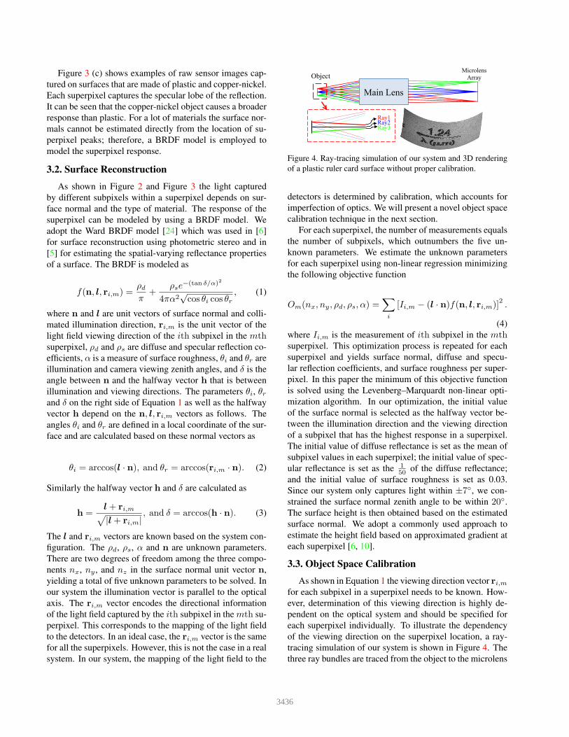
Figure 3 (c) shows examples of raw sensor images cap-

tured on surfaces that are made of plastic and copper-nickel.

Each superpixel captures the specular lobe of the reflection.

It can be seen that the copper-nickel object causes a broader

response than plastic. For a lot of materials the surface nor-

mals cannot be estimated directly from the location of su-

perpixel peaks; therefore, a BRDF model is employed to

model the superpixel response.

3.2. Surface Reconstruction

As shown in Figure 2 and Figure 3 the light captured

by different subpixels within a superpixel depends on sur-

face normal and the type of material. The response of the

superpixel can be modeled by using a BRDF model. We

adopt the Ward BRDF model [24] which was used in [6]

for surface reconstruction using photometric stereo and in

[5] for estimating the spatial-varying reflectance properties

of a surface. The BRDF is modeled as

f(n, l, ri,m) =ρdπ

+ρse

−(tan δ/α)2

4πα2√cos θi cos θr

, (1)

where n and l are unit vectors of surface normal and colli-

mated illumination direction, ri,m is the unit vector of the

light field viewing direction of the ith subpixel in the mthsuperpixel, ρd and ρs are diffuse and specular reflection co-

efficients, α is a measure of surface roughness, θi and θr are

illumination and camera viewing zenith angles, and δ is the

angle between n and the halfway vector h that is between

illumination and viewing directions. The parameters θi, θrand δ on the right side of Equation 1 as well as the halfway

vector h depend on the n, l, ri,m vectors as follows. The

angles θi and θr are defined in a local coordinate of the sur-

face and are calculated based on these normal vectors as

θi = arccos(l · n), and θr = arccos(ri,m · n). (2)

Similarly the halfway vector h and δ are calculated as

h =l+ ri,m

p

|l+ ri,m|, and δ = arccos(h · n). (3)

The l and ri,m vectors are known based on the system con-

figuration. The ρd, ρs, α and n are unknown parameters.

There are two degrees of freedom among the three compo-

nents nx, ny , and nz in the surface normal unit vector n,

yielding a total of five unknown parameters to be solved. In

our system the illumination vector is parallel to the optical

axis. The ri,m vector encodes the directional information

of the light field captured by the ith subpixel in the mth su-

perpixel. This corresponds to the mapping of the light field

to the detectors. In an ideal case, the ri,m vector is the same

for all the superpixels. However, this is not the case in a real

system. In our system, the mapping of the light field to the

Main Lens

Object Microlens

Array

Ray1 Ray2 Ray3

Figure 4. Ray-tracing simulation of our system and 3D rendering

of a plastic ruler card surface without proper calibration.

detectors is determined by calibration, which accounts for

imperfection of optics. We will present a novel object space

calibration technique in the next section.

For each superpixel, the number of measurements equals

the number of subpixels, which outnumbers the five un-

known parameters. We estimate the unknown parameters

for each superpixel using non-linear regression minimizing

the following objective function

Om(nx, ny, ρd, ρs, α) =X

i

[Ii,m − (l · n)f(n, l, ri,m)]2.

(4)

where Ii,m is the measurement of ith subpixel in the mthsuperpixel. This optimization process is repeated for each

superpixel and yields surface normal, diffuse and specu-

lar reflection coefficients, and surface roughness per super-

pixel. In this paper the minimum of this objective function

is solved using the Levenberg–Marquardt non-linear opti-

mization algorithm. In our optimization, the initial value

of the surface normal is selected as the halfway vector be-

tween the illumination direction and the viewing direction

of a subpixel that has the highest response in a superpixel.

The initial value of diffuse reflectance is set as the mean of

subpixel values in each superpixel; the initial value of spec-

ular reflectance is set as the 150 of the diffuse reflectance;

and the initial value of surface roughness is set as 0.03.

Since our system only captures light within ±7◦, we con-

strained the surface normal zenith angle to be within 20◦.

The surface height is then obtained based on the estimated

surface normal. We adopt a commonly used approach to

estimate the height field based on approximated gradient at

each superpixel [6, 10].

3.3. Object Space Calibration

As shown in Equation 1 the viewing direction vector ri,mfor each subpixel in a superpixel needs to be known. How-

ever, determination of this viewing direction is highly de-

pendent on the optical system and should be specified for

each superpixel individually. To illustrate the dependency

of the viewing direction on the superpixel location, a ray-

tracing simulation of our system is shown in Figure 4. The

three ray bundles are traced from the object to the microlens

3436

On-axis

Off-axis

θr (zenith angle) Φr (azimuth angle)

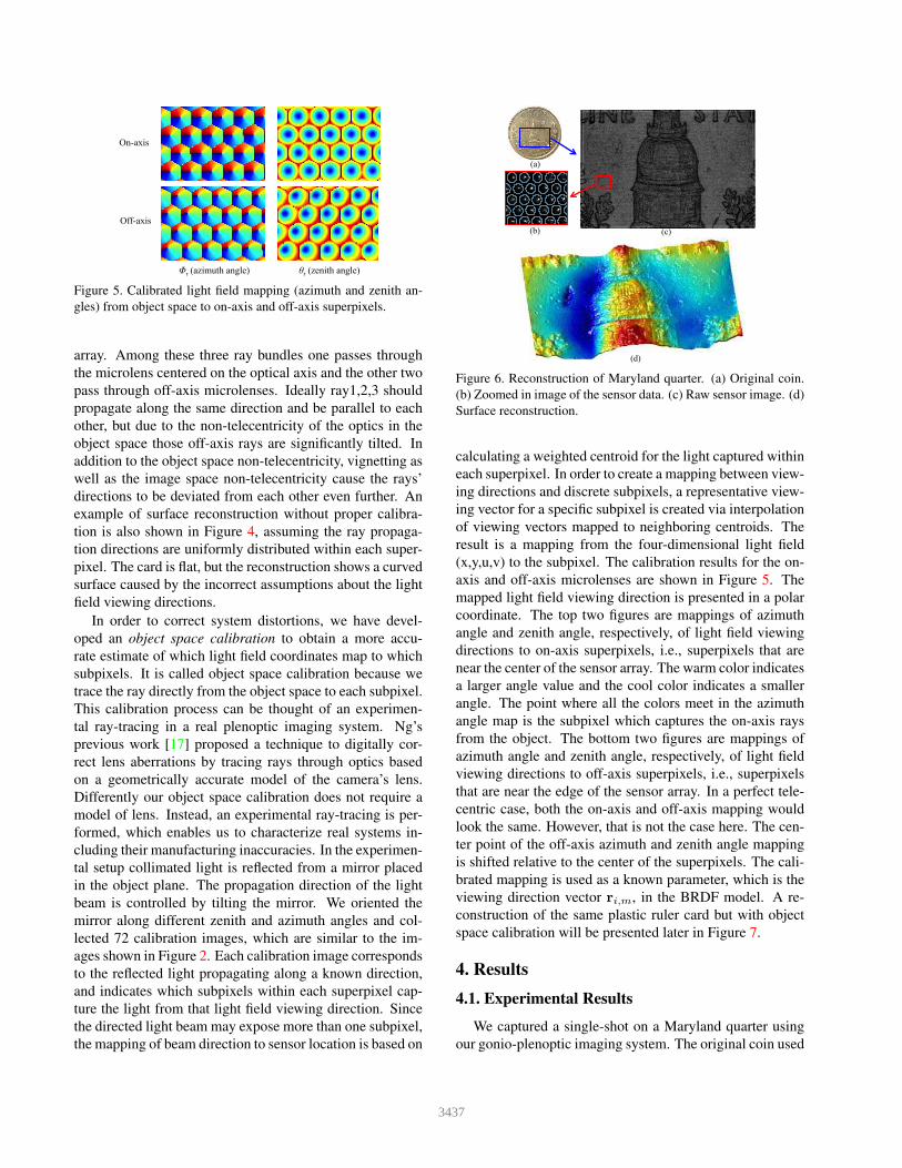
Figure 5. Calibrated light field mapping (azimuth and zenith an-

gles) from object space to on-axis and off-axis superpixels.

array. Among these three ray bundles one passes through

the microlens centered on the optical axis and the other two

pass through off-axis microlenses. Ideally ray1,2,3 should

propagate along the same direction and be parallel to each

other, but due to the non-telecentricity of the optics in the

object space those off-axis rays are significantly tilted. In

addition to the object space non-telecentricity, vignetting as

well as the image space non-telecentricity cause the rays’

directions to be deviated from each other even further. An

example of surface reconstruction without proper calibra-

tion is also shown in Figure 4, assuming the ray propaga-

tion directions are uniformly distributed within each super-

pixel. The card is flat, but the reconstruction shows a curved

surface caused by the incorrect assumptions about the light

field viewing directions.

In order to correct system distortions, we have devel-

oped an object space calibration to obtain a more accu-

rate estimate of which light field coordinates map to which

subpixels. It is called object space calibration because we

trace the ray directly from the object space to each subpixel.

This calibration process can be thought of an experimen-

tal ray-tracing in a real plenoptic imaging system. Ng’s

previous work [17] proposed a technique to digitally cor-

rect lens aberrations by tracing rays through optics based

on a geometrically accurate model of the camera’s lens.

Differently our object space calibration does not require a

model of lens. Instead, an experimental ray-tracing is per-

formed, which enables us to characterize real systems in-

cluding their manufacturing inaccuracies. In the experimen-

tal setup collimated light is reflected from a mirror placed

in the object plane. The propagation direction of the light

beam is controlled by tilting the mirror. We oriented the

mirror along different zenith and azimuth angles and col-

lected 72 calibration images, which are similar to the im-

ages shown in Figure 2. Each calibration image corresponds

to the reflected light propagating along a known direction,

and indicates which subpixels within each superpixel cap-

ture the light from that light field viewing direction. Since

the directed light beam may expose more than one subpixel,

the mapping of beam direction to sensor location is based on

(a)

(c)

(d)

(b)

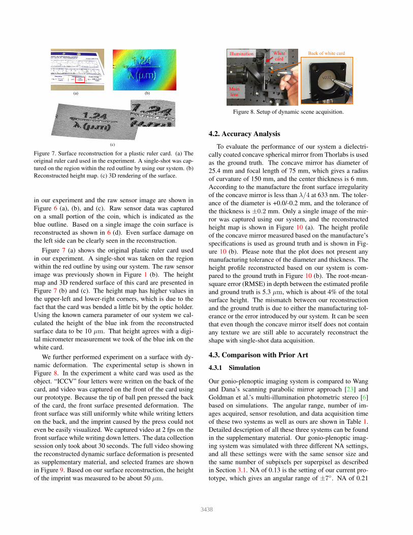
Figure 6. Reconstruction of Maryland quarter. (a) Original coin.

(b) Zoomed in image of the sensor data. (c) Raw sensor image. (d)

Surface reconstruction.

calculating a weighted centroid for the light captured within

each superpixel. In order to create a mapping between view-

ing directions and discrete subpixels, a representative view-

ing vector for a specific subpixel is created via interpolation

of viewing vectors mapped to neighboring centroids. The

result is a mapping from the four-dimensional light field

(x,y,u,v) to the subpixel. The calibration results for the on-

axis and off-axis microlenses are shown in Figure 5. The

mapped light field viewing direction is presented in a polar

coordinate. The top two figures are mappings of azimuth

angle and zenith angle, respectively, of light field viewing

directions to on-axis superpixels, i.e., superpixels that are

near the center of the sensor array. The warm color indicates

a larger angle value and the cool color indicates a smaller

angle. The point where all the colors meet in the azimuth

angle map is the subpixel which captures the on-axis rays

from the object. The bottom two figures are mappings of

azimuth angle and zenith angle, respectively, of light field

viewing directions to off-axis superpixels, i.e., superpixels

that are near the edge of the sensor array. In a perfect tele-

centric case, both the on-axis and off-axis mapping would

look the same. However, that is not the case here. The cen-

ter point of the off-axis azimuth and zenith angle mapping

is shifted relative to the center of the superpixels. The cali-

brated mapping is used as a known parameter, which is the

viewing direction vector ri,m, in the BRDF model. A re-

construction of the same plastic ruler card but with object

space calibration will be presented later in Figure 7.

4. Results

4.1. Experimental Results

We captured a single-shot on a Maryland quarter using

our gonio-plenoptic imaging system. The original coin used

3437

(b) (a)

(c)

Figure 7. Surface reconstruction for a plastic ruler card. (a) The

original ruler card used in the experiment. A single-shot was cap-

tured on the region within the red outline by using our system. (b)

Reconstructed height map. (c) 3D rendering of the surface.

in our experiment and the raw sensor image are shown in

Figure 6 (a), (b), and (c). Raw sensor data was captured

on a small portion of the coin, which is indicated as the

blue outline. Based on a single image the coin surface is

reconstructed as shown in 6 (d). Even surface damage on

the left side can be clearly seen in the reconstruction.

Figure 7 (a) shows the original plastic ruler card used

in our experiment. A single-shot was taken on the region

within the red outline by using our system. The raw sensor

image was previously shown in Figure 1 (b). The height

map and 3D rendered surface of this card are presented in

Figure 7 (b) and (c). The height map has higher values in

the upper-left and lower-right corners, which is due to the

fact that the card was bended a little bit by the optic holder.

Using the known camera parameter of our system we cal-

culated the height of the blue ink from the reconstructed

surface data to be 10 µm. That height agrees with a digi-

tal micrometer measurement we took of the blue ink on the

white card.

We further performed experiment on a surface with dy-

namic deformation. The experimental setup is shown in

Figure 8. In the experiment a white card was used as the

object. “ICCV” four letters were written on the back of the

card, and video was captured on the front of the card using

our prototype. Because the tip of ball pen pressed the back

of the card, the front surface presented deformation. The

front surface was still uniformly white while writing letters

on the back, and the imprint caused by the press could not

even be easily visualized. We captured video at 2 fps on the

front surface while writing down letters. The data collection

session only took about 30 seconds. The full video showing

the reconstructed dynamic surface deformation is presented

as supplementary material, and selected frames are shown

in Figure 9. Based on our surface reconstruction, the height

of the imprint was measured to be about 50 µm.

Illumination

Main

lens

White

card

Back of white card

Figure 8. Setup of dynamic scene acquisition.

4.2. Accuracy Analysis

To evaluate the performance of our system a dielectri-

cally coated concave spherical mirror from Thorlabs is used

as the ground truth. The concave mirror has diameter of

25.4 mm and focal length of 75 mm, which gives a radius

of curvature of 150 mm, and the center thickness is 6 mm.

According to the manufacture the front surface irregularity

of the concave mirror is less than λ/4 at 633 nm. The toler-

ance of the diameter is +0.0/-0.2 mm, and the tolerance of

the thickness is ±0.2 mm. Only a single image of the mir-

ror was captured using our system, and the reconstructed

height map is shown in Figure 10 (a). The height profile

of the concave mirror measured based on the manufacture’s

specifications is used as ground truth and is shown in Fig-

ure 10 (b). Please note that the plot does not present any

manufacturing tolerance of the diameter and thickness. The

height profile reconstructed based on our system is com-

pared to the ground truth in Figure 10 (b). The root-mean-

square error (RMSE) in depth between the estimated profile

and ground truth is 5.3 µm, which is about 4% of the total

surface height. The mismatch between our reconstruction

and the ground truth is due to either the manufacturing tol-

erance or the error introduced by our system. It can be seen

that even though the concave mirror itself does not contain

any texture we are still able to accurately reconstruct the

shape with single-shot data acquisition.

4.3. Comparison with Prior Art

4.3.1 Simulation

Our gonio-plenoptic imaging system is compared to Wang

and Dana’s scanning parabolic mirror approach [23] and

Goldman et al.’s multi-illumination photometric stereo [6]

based on simulations. The angular range, number of im-

ages acquired, sensor resolution, and data acquisition time

of these two systems as well as ours are shown in Table 1.

Detailed description of all these three systems can be found

in the supplementary material. Our gonio-plenoptic imag-

ing system was simulated with three different NA settings,

and all these settings were with the same sensor size and

the same number of subpixels per superpixel as described

in Section 3.1. NA of 0.13 is the setting of our current pro-

totype, which gives an angular range of ±7◦. NA of 0.21

3438

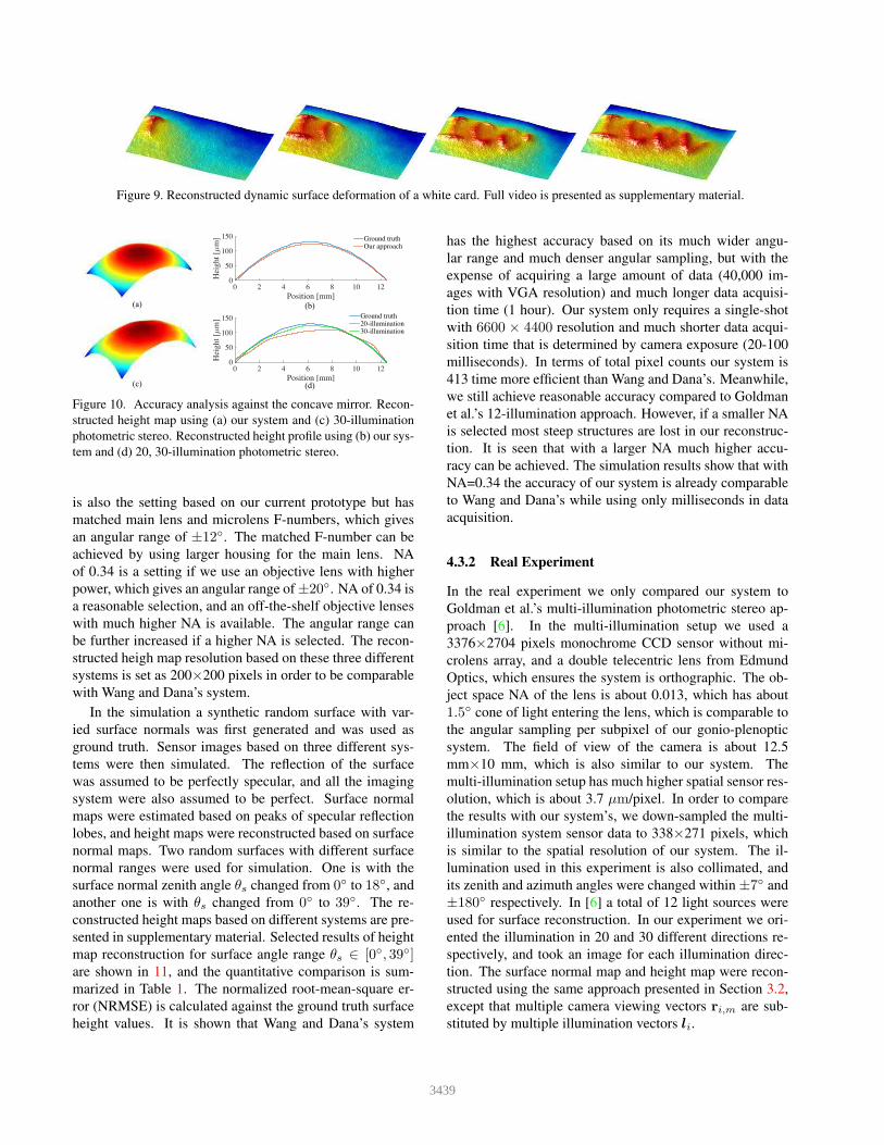
Figure 9. Reconstructed dynamic surface deformation of a white card. Full video is presented as supplementary material.

Position [mm]0 2 4 6 8 10 12

Hei

gh

t [7

m]

0

50

100

150 Ground truthOur approach

Position [mm]0 2 4 6 8 10 12

Hei

gh

t [7

m]

0

50

100

150 Ground truth20-illumination30-illumination

(a) (b)

(d) (c)

Figure 10. Accuracy analysis against the concave mirror. Recon-

structed height map using (a) our system and (c) 30-illumination

photometric stereo. Reconstructed height profile using (b) our sys-

tem and (d) 20, 30-illumination photometric stereo.

is also the setting based on our current prototype but has

matched main lens and microlens F-numbers, which gives

an angular range of ±12◦. The matched F-number can be

achieved by using larger housing for the main lens. NA

of 0.34 is a setting if we use an objective lens with higher

power, which gives an angular range of ±20◦. NA of 0.34 is

a reasonable selection, and an off-the-shelf objective lenses

with much higher NA is available. The angular range can

be further increased if a higher NA is selected. The recon-

structed heigh map resolution based on these three different

systems is set as 200×200 pixels in order to be comparable

with Wang and Dana’s system.

In the simulation a synthetic random surface with var-

ied surface normals was first generated and was used as

ground truth. Sensor images based on three different sys-

tems were then simulated. The reflection of the surface

was assumed to be perfectly specular, and all the imaging

system were also assumed to be perfect. Surface normal

maps were estimated based on peaks of specular reflection

lobes, and height maps were reconstructed based on surface

normal maps. Two random surfaces with different surface

normal ranges were used for simulation. One is with the

surface normal zenith angle θs changed from 0◦ to 18◦, and

another one is with θs changed from 0◦ to 39◦. The re-

constructed height maps based on different systems are pre-

sented in supplementary material. Selected results of height

map reconstruction for surface angle range θs ∈ [0◦, 39◦]are shown in 11, and the quantitative comparison is sum-

marized in Table 1. The normalized root-mean-square er-

ror (NRMSE) is calculated against the ground truth surface

height values. It is shown that Wang and Dana’s system

has the highest accuracy based on its much wider angu-

lar range and much denser angular sampling, but with the

expense of acquiring a large amount of data (40,000 im-

ages with VGA resolution) and much longer data acquisi-

tion time (1 hour). Our system only requires a single-shot

with 6600 × 4400 resolution and much shorter data acqui-

sition time that is determined by camera exposure (20-100

milliseconds). In terms of total pixel counts our system is

413 time more efficient than Wang and Dana’s. Meanwhile,

we still achieve reasonable accuracy compared to Goldman

et al.’s 12-illumination approach. However, if a smaller NA

is selected most steep structures are lost in our reconstruc-

tion. It is seen that with a larger NA much higher accu-

racy can be achieved. The simulation results show that with

NA=0.34 the accuracy of our system is already comparable

to Wang and Dana’s while using only milliseconds in data

acquisition.

4.3.2 Real Experiment

In the real experiment we only compared our system to

Goldman et al.’s multi-illumination photometric stereo ap-

proach [6]. In the multi-illumination setup we used a

3376×2704 pixels monochrome CCD sensor without mi-

crolens array, and a double telecentric lens from Edmund

Optics, which ensures the system is orthographic. The ob-

ject space NA of the lens is about 0.013, which has about

1.5◦ cone of light entering the lens, which is comparable to

the angular sampling per subpixel of our gonio-plenoptic

system. The field of view of the camera is about 12.5

mm×10 mm, which is also similar to our system. The

multi-illumination setup has much higher spatial sensor res-

olution, which is about 3.7 µm/pixel. In order to compare

the results with our system’s, we down-sampled the multi-

illumination system sensor data to 338×271 pixels, which

is similar to the spatial resolution of our system. The il-

lumination used in this experiment is also collimated, and

its zenith and azimuth angles were changed within ±7◦ and

±180◦ respectively. In [6] a total of 12 light sources were

used for surface reconstruction. In our experiment we ori-

ented the illumination in 20 and 30 different directions re-

spectively, and took an image for each illumination direc-

tion. The surface normal map and height map were recon-

structed using the same approach presented in Section 3.2,

except that multiple camera viewing vectors ri,m are sub-

stituted by multiple illumination vectors li.

3439

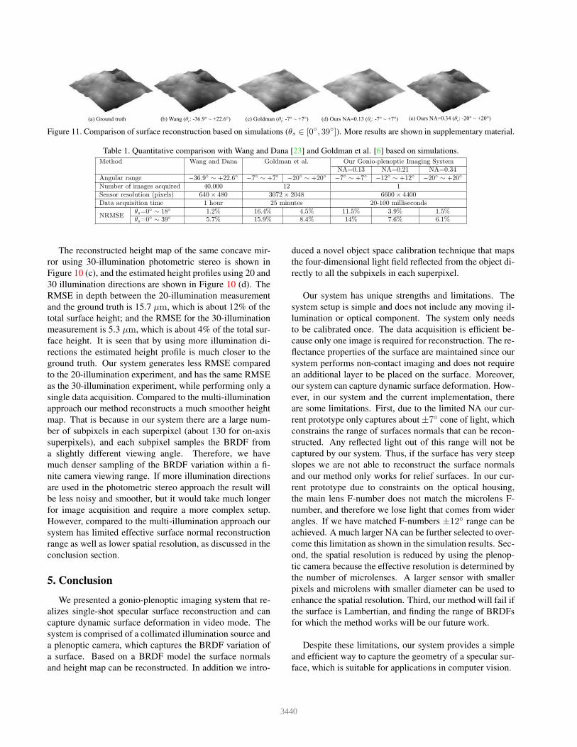
(a) Ground truth (b) Wang (θr: -36.9° ~ +22.6°) (d) Ours NA=0.13 (θ

r: -7° ~ +7°) (e) Ours NA=0.34 (θ

r: -20° ~ +20°) (c) Goldman (θ

i: -7° ~ +7°)

Figure 11. Comparison of surface reconstruction based on simulations (θs ∈ [0◦, 39◦]). More results are shown in supplementary material.

Table 1. Quantitative comparison with Wang and Dana [23] and Goldman et al. [6] based on simulations.

Method Wang and Dana Goldman et al. Our Gonio-plenoptic Imaging SystemNA=0.13 NA=0.21 NA=0.34

Angular range −36.9◦ ∼ +22.6◦ −7◦ ∼ +7◦ −20◦ ∼ +20◦ −7◦ ∼ +7◦ −12◦ ∼ +12◦ −20◦ ∼ +20◦

Number of images acquired 40,000 12 1Sensor resolution (pixels) 640× 480 3072× 2048 6600× 4400Data acquisition time 1 hour 25 minutes 20-100 milliseconds

NRMSEθs=0◦ ∼ 18◦ 1.2% 16.4% 4.5% 11.5% 3.9% 1.5%θs=0◦ ∼ 39◦ 5.7% 15.9% 8.4% 14% 7.6% 6.1%

The reconstructed height map of the same concave mir-

ror using 30-illumination photometric stereo is shown in

Figure 10 (c), and the estimated height profiles using 20 and

30 illumination directions are shown in Figure 10 (d). The

RMSE in depth between the 20-illumination measurement

and the ground truth is 15.7 µm, which is about 12% of the

total surface height; and the RMSE for the 30-illumination

measurement is 5.3 µm, which is about 4% of the total sur-

face height. It is seen that by using more illumination di-

rections the estimated height profile is much closer to the

ground truth. Our system generates less RMSE compared

to the 20-illumination experiment, and has the same RMSE

as the 30-illumination experiment, while performing only a

single data acquisition. Compared to the multi-illumination

approach our method reconstructs a much smoother height

map. That is because in our system there are a large num-

ber of subpixels in each superpixel (about 130 for on-axis

superpixels), and each subpixel samples the BRDF from

a slightly different viewing angle. Therefore, we have

much denser sampling of the BRDF variation within a fi-

nite camera viewing range. If more illumination directions

are used in the photometric stereo approach the result will

be less noisy and smoother, but it would take much longer

for image acquisition and require a more complex setup.

However, compared to the multi-illumination approach our

system has limited effective surface normal reconstruction

range as well as lower spatial resolution, as discussed in the

conclusion section.

5. Conclusion

We presented a gonio-plenoptic imaging system that re-

alizes single-shot specular surface reconstruction and can

capture dynamic surface deformation in video mode. The

system is comprised of a collimated illumination source and

a plenoptic camera, which captures the BRDF variation of

a surface. Based on a BRDF model the surface normals

and height map can be reconstructed. In addition we intro-

duced a novel object space calibration technique that maps

the four-dimensional light field reflected from the object di-

rectly to all the subpixels in each superpixel.

Our system has unique strengths and limitations. The

system setup is simple and does not include any moving il-

lumination or optical component. The system only needs

to be calibrated once. The data acquisition is efficient be-

cause only one image is required for reconstruction. The re-

flectance properties of the surface are maintained since our

system performs non-contact imaging and does not require

an additional layer to be placed on the surface. Moreover,

our system can capture dynamic surface deformation. How-

ever, in our system and the current implementation, there

are some limitations. First, due to the limited NA our cur-

rent prototype only captures about ±7◦ cone of light, which

constrains the range of surfaces normals that can be recon-

structed. Any reflected light out of this range will not be

captured by our system. Thus, if the surface has very steep

slopes we are not able to reconstruct the surface normals

and our method only works for relief surfaces. In our cur-

rent prototype due to constraints on the optical housing,

the main lens F-number does not match the microlens F-

number, and therefore we lose light that comes from wider

angles. If we have matched F-numbers ±12◦ range can be

achieved. A much larger NA can be further selected to over-

come this limitation as shown in the simulation results. Sec-

ond, the spatial resolution is reduced by using the plenop-

tic camera because the effective resolution is determined by

the number of microlenses. A larger sensor with smaller

pixels and microlens with smaller diameter can be used to

enhance the spatial resolution. Third, our method will fail if

the surface is Lambertian, and finding the range of BRDFs

for which the method works will be our future work.

Despite these limitations, our system provides a simple

and efficient way to capture the geometry of a specular sur-

face, which is suitable for applications in computer vision.

3440

References

[1] E. H. Adelson and J. Y. A. Wang. Single lens

stereo with a plenoptic camera. IEEE Trans. PAMI,

14(2):99–106, 1992. 1, 2

[2] R. Basri, D. Jacobs, and I. Kemelmacher. Photometric

stereo with general, unknown lighting. International

Journal of Computer Vision, 72(3):239–257, 2007. 2

[3] T. Chen, M. Goesele, and H.-P. Seidel. Mesostructure

from specularity. In Proc. CVPR, pages 1825–1832,

2006. 2

[4] Y. Francken, T. Cuypers, T. Mertens, J. Gielis, and

P. Bekaert. High quality mesostructure acquisition us-

ing specularities. In Proc. CVPR, pages 1–7, 2008.

2

[5] A. Gardner, C. Tchou, T. Hawkins, and P. Debevec.

Linear light source reflectometry. In ACM Trans.

Graph., number 3, pages 749–758. ACM, 2003. 2,

3.2

[6] D. B. Goldman, B. Curless, A. Hertzmann, and S. M.

Seitz. Shape and spatially-varying BRDFs from pho-

tometric stereo. IEEE Trans. PAMI, 32(6):1060–1071,

2010. 1, 2, 3.2, 3.2, 4.3.1, 4.3.2, 1

[7] A. Hertzmann and S. M. Seitz. Example-based pho-

tometric stereo: Shape reconstruction with general,

varying BRDFs. IEEE Trans. PAMI, 27(8):1254–

1264, 2005. 1, 2

[8] Y. Ji, J. Ye, and J. Yu. Reconstructing gas flows us-

ing light-path approximation. In Proc. CVPR, pages

2507–2514, 2013. 2

[9] H. Jin, S. Soatto, and A. J. Yezzi. Multi-view stereo

beyond Lambert. In Proc. CVPR, pages I–171–I–178,

2003. 2

[10] M. K. Johnson and E. H. Adelson. Retrographic sens-

ing for the measurement of surface texture and shape.

In Proc. CVPR, pages 1070–1077, 2009. 1, 2, 3.2

[11] M. K. Johnson, F. Cole, A. Raj, and E. H. Adelson.

Microgeometry capture using an elastomeric sensor.

ACM Trans. Graph., 30(4):46:1–46:8, July 2011. 1, 2

[12] M. Levoy, R. Ng, A. Adams, M. Footer, and

M. Horowitz. Light field microscopy. ACM Trans.

Graph., 25(3):924–934, July 2006. 2

[13] M. Levoy, Z. Zhang, and I. McDowall. Recording and

controlling the 4d light field in a microscope using mi-

crolens arrays. Journal of Microscopy, 235(2):144–

162, 2009. 2

[14] A. Lumsdaine and T. Georgiev. The focused plenoptic

camera. In Proc. ICCP, pages 1–8, 2009. 2

[15] C. Ma, X. Lin, J. Suo, Q. Dai, and G. Wetzstein.

Transparent object reconstruction via coded transport

of intensity. In Proc. CVPR, pages 3238–3245, 2014.

2

[16] S. K. Nayar, A. C. Sanderson, L. E. Weiss, and D. A.

Simon. Specular surface inspection using structured

highlight and gaussian images. IEEE Trans. Robot.

Autom., 6(2):208–218, 1990. 2

[17] R. Ng. Digital light field photography. PhD thesis,

Stanford University, 2006. 3.3

[18] R. Ng, M. Levoy, M. Bredif, G. Duval, M. Horowitz,

and P. Hanrahan. Light field photography with a hand-

held plenoptic camera. Tech. rep., Stanford University,

2005. 2

[19] F. Pernkopf and P. O’Leary. Image acquisition tech-

niques for automatic visual inspection of metallic sur-

faces. NDT & E International, 36(8):609–617, 2003.

1

[20] C. Perwaß and L. Wietzke. Single lens 3D-camera

with extended depth-of-field. In IS&T/SPIE Elec-

tronic Imaging, pages 829108–829108, 2012. 1, 2

[21] B. C. Platt and R. Shack. History and principles of

Shack-Hartmann wavefront sensing. Journal of Re-

fractive Surgery, 17(5):S573–S577, 2001. 2

[22] I. Tosic and K. Berkner. Light field scale-depth

space transform for dense depth estimation. In Proc.

CVPRW, pages 441–448, 2014. 1

[23] J. Wang and K. J. Dana. Relief texture from specular-

ities. IEEE Trans. PAMI, 28(3):446–457, 2006. 1, 2,

4.3.1, 1

[24] G. J. Ward. Measuring and modeling anisotropic re-

flection. Computer Graphics, 26(2):265–272, 1992.

3.2

[25] G. Wetzstein, D. Roodnick, W. Heidrich, and

R. Raskar. Refractive shape from light field distor-

tion. In Proc. ICCV, pages 1180–1186. IEEE, 2011.

2

[26] R. J. Woodham. Photometric method for determining

surface orientation from multiple images. Optical En-

gineering, 19(1):191139–191139, 1980. 2

[27] T. Yu, N. Xu, and N. Ahuja. Recovering shape and re-

flectance model of non-lambertian objects from mul-

tiple views. In Proc. CVPR, volume 2, pages II–226–

II–233, 2004. 2

3441