NASA Technical Memorandum 86832

NASA-TM-8683219860011463

Simulation of Landsat Multispectral Scanner Spatial Resolution with Airborne Scanner Data Christine A. Hlavka

January 1986

NI\S/\ National Aeronautics and Space Administration 1111111111111 IIII 11111 11111 11111 11111 IIII 1111

NF00074

https://ntrs.nasa.gov/search.jsp?R=19860011463 2018-08-19T11:46:58+00:00Z

NASA Technical Memorandum 86832

Simulation of Landsat Multispectral Scanner Spatial Resolution with Airborne Scanner Data Christine A. Hlavka, Ames Research Center, Moffett Field, California

January 1986

1/\5/\ National Aeronautics and Space Administration

Ames Research Center Moffett Field, California 94035

SUMMARY

A technique for simulation of low spatial resolution satellite imagery by using high resolution scanner data is described. The scanner data is convolved with the approximate pOint spread function of the low resolution data and then resampled to emulate low resolution imagery. The technique was successfully applied to Daedalus airborne scanner data to simulate a portion of a Landsat multispectral scanner scene.

INTRODUCTION

Satellite data is often simulated by using airborne scanner data in investiga­tions into the utility of various imaging system characteristics. These investiga­tions provide important information for the assessment of operational satellite data and the design of future imaging systems.

Daedalus Airborne Thematic Mapper (ATM) imagery was used to study the effects of Thematic Mapper (TM) characteristics on the accuracy of land use and land cover classifications (ref. 1). Seven ATM bands were configured to match TM bands 1-7. A mosaic showing portions of several flight lines was used to simulate a TM scene. This data set was systematically degraded to simulate multispectral scanner (MSS) imagery. Six other data sets combining MSS and TM characteristics were also gener­ated so that all possible combinations of MSS or TM spatial, spectral, and radio­metric resolutions could be tested.

The procedures for simulating MSS spatial resolution with ATM imagery will be described. Simulation of low spatial resolution is often achieved by boxcar filter­ing. (Each simulated low resolution pixel is given the average brightness value of a rectangular neighborhood of pixels on the high resolution data (refs. 2 and 3).) This degrades the resolution excessively, because too much weight is given to pixels away from the center of the instantaneous field of view (IFOV). An improved proce­dure described here uses published estimates of the modulation transfer function (MTF) of Landsat MSS to determine the optimal coefficients in a weighted averaging.

SIMULATION OF LOW SPATIAL RESOLUTION

The object of an optical system such as a scanner can be represented as a continuous function f(x,y), the radiation emitted and reflected at point (x,y). The proportion of reflectance as a function P(a,b) of distance (a,b) from the center of a pixel is the system point spread function (PSF). If geometric distor-

tions and noise are not present or are ignored, then the grey level is modeled as the convolution of f(x,y) and P(a,b):

g(x,y) = f_: f_: f(x - a, y - b) ·P(a,b)da db ( 1 )

Equation (1) implies that the PSF is constant over time and space, which is approxi­matel.y true, although this may vary somewhat with changes in atmospheric condi­tions. For a more complete discussion of image formation, the reader is referred to Moik (ref. 4) and Schowengerdt (ref. 5).

The PSF of a scanner system has an approximately Gaussian shape (refs. 4 and 5):

with P(O,O) = C at the center and P(WX,O) = P(O,WY) = C/2, where:

are the half maximum pOints in the two directions.

An image g(x,y) of coarse resolution can be simulated by using a fine resolu­tion image F(x,y) in place of f(x,y) and performing discrete convolution:

n m g(x,y) = ~ ~ F(x - i,y - j)·P(i,j)

i=-n j=-m

with the numbers nand m chosen so that P(i,j) is small outside the (2n + 1)x(2m + 1) convolution window.

(2)

One may ask how fine a resolution is needed so that F(x,y) approximates f(x,y) sufficiently well for the simulation operation represented in equation (2). The high resolution grey-level value F(x,y) is the convolution of f(x,y) with the PSF of the high resolution system P'(a,b). The low resolution grey value g(x,y) can be expressed as the convolution of F(x,y) with a relative PSF (ref. 6). The appropriate PSF is the inverse Fourier transform of the ratio of the MTFs of the scanners (ref. 6). If P'(a,b) is Gaussian:

P' (a,b) 2 2 = C'.exp(-k;.a ).exp(-k2·b )

then P"(a,b) is also Gaussian:

P"(a,b)

2

with k" = k ·k'/(k - k') and 1 0 1 1 0 1 1 11 to utlon system IS severa Imes then k; «k1 and k2« k2' and k2 .

k2 = k 'k2/(k2 - k2). If the IFOV of the low reso­larger €han that of the high resolution system, and thus k1 and k2 are approximately equal to k1

Since convolution is a central-processing-unit-intensive computer operation, an alternative approach was considered. Low spatial resolution can be simulated in the Fourier frequency domain by multiplying the Fourier transform of the high resolution imagery by the MTF of the low resolution imagery, and then taking the inverse trans­form. This is often more efficient computationally (ref. 7), but software for Fourier processing is often limited to images whose dimensions are powers of two. If an image is inserted into a background image in order to create an image of allowable dimensions, great care must be taken to avoid "ringing" caused by discon­tinuities in brightness values (ref. 4). These difficulties are avoided in the convolution procedure, so it was adopted despite its inefficiency.

Equation (2) is implemented in three steps:

Step 1. Generate a Gauss filter with parameters WX and WY computed from the low resolution PSF, with C = 1.0, and large dimensions compared to the low resolu­tion IFOV. This filter is used to compute the appropriate normalizing constant C and filter dimensions for the convolution filter. A simple rule is to use a central rectangular portion of the filter which retains all values of 0.10 or greater. The normalizing value C is recalculated as the inverse of the sum of values of the selected portion, so that the magnitude of the grey levels will remain approximately the same after convolution.

Step 2. The high resolution scanner data is convolved with this filter.

Step 3. The image is resampled using nearest neighbor grey-level values so that pixel spacings correspond to those of the low resolution imagery. Bilinear or bicubic resampling should not be used because the resolution would be broadened by the interpolation process.

SIMULATION OF MSS WITH SCANNER DATA

Landsat MSS imagery was simulated by using Daedalus airborne Thematic Mapper imagery collected during a U-2 flight over central California. The IFOV of the scanner was 1.25 mrad, or 25 m at an altitude of 65,000 ft. Measurements on the imagery determined that pixel spacings were 17 m along scan and 22 m along track.

The PSF of Landsat was approximated using published results of Fourier analysis of MSS imagery (ref. 8). MTF values at multiples of approximately 1.5 cycles per kilometer were measured on graphs of the MTF as a function of frequency in the along-scan and along-track directions. These were fit to Gaussian curves by linear regressions of the logarithm of the MTF versus square of the frequency. The MTF was:

.3

2 2 M(u,v) = M(u)·M(v) = exp(-0.0233·u )·exp(-0.0185·v )

where u and v are frequencies in the along-scan and along-track directions in cycles per kilometer. The PSF was calculated by taking the inverse Fourier trans­form of the MTF. This PSF was Gaussian with spread parameters:

k1 = n2/0.0185 = 532.5 km-2

WX = 36.1 m and WY = 40.1 m

and 2 k2 = n 10.0233 = 424.4 km-2

These half maximum points are approximately half the 79 m IFOV of MSS.

IMPLEMENTATION OF IOIMS

The software program, Interactive Oigital Image Manipulation (IOIMS) (ESL Incorporated, Sunnyvale, California), was used to simulate low spatial resolution of MSS (ref. 9). IOIMS software for creating filters is normally used for filtering in the Fourier domain, therefore the half maximum points had to be converted to units of cycles per pixel. Let WX' and WY' be in units of ground distance (meters). Let the pixel spacings of the high resolution imagery be dx and dy. The size of the filter was initially chosen to be 32 lines by 32 samples. The filter parameters for the IDIMS program GAUSS were:

WX = WX'/(ns·dx) = 36.1/(32·17) = 0.0665

WY = WY'/(nl·dy) = 40.1/(32·22) = 0.0582

OCGAIN = C = 1.0 HFGAIN = 0.0

NL = 32 NS = 32

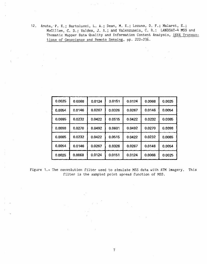
All values outside of the 7x7 center of the resulting image were less than 0.10. The sum of values in the 7x7 center was 16.64, therefore C was recalculated to be 1/16.64 = 0.0601. The GAUSS program was rerun with DCGAIN = 0.0601 (keeping the other parameters the same), and the 7x7 center of the resulting image (see fig. 1) was used as the convolution filter. Convolution was performed by running the CONVOL program with the Daedalus data and the filter as input images.

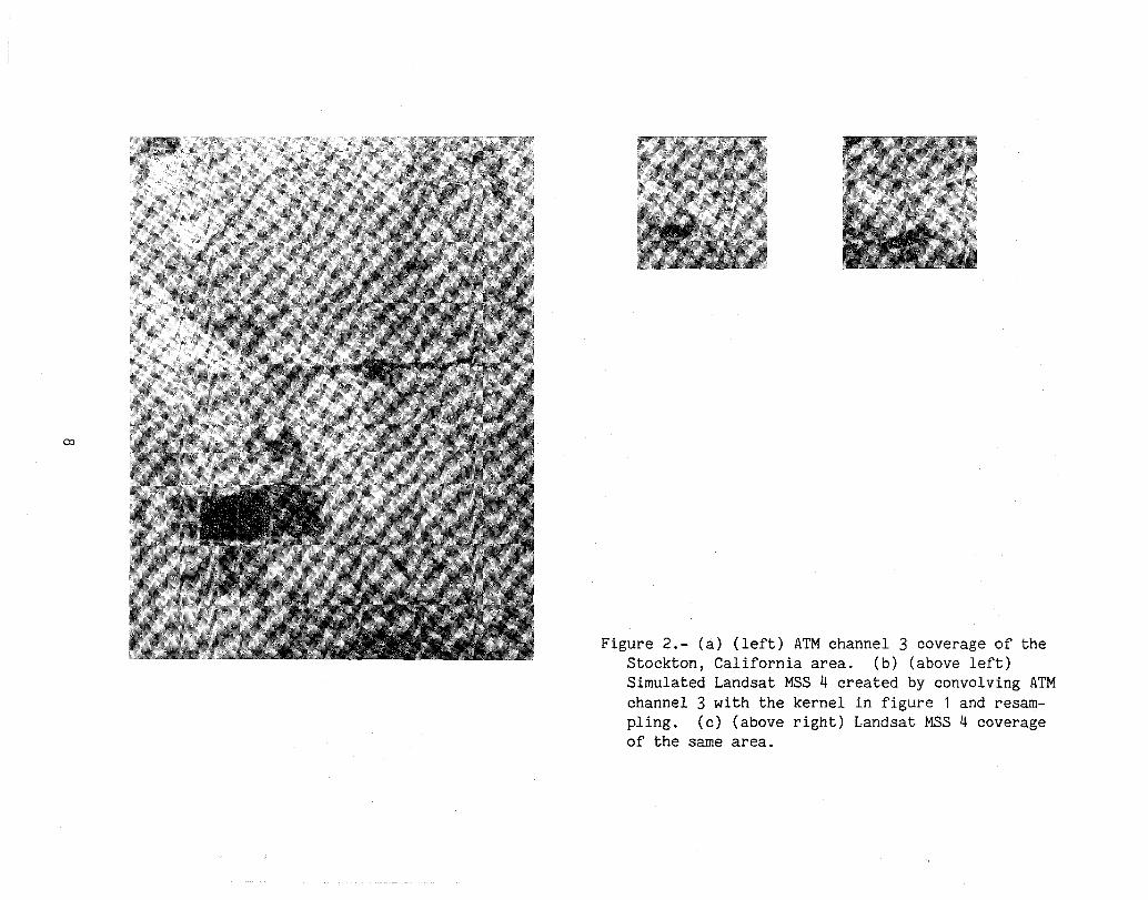
The convolved image was resampled to approximate the MSS pixel spacings of 57 m x 57 m computer compatible tapes. Every fourth line and every third pixel was sampled to create an image with 68 m x 66 m pixel spacings using the MAGNIFY program with LINEFACT = 0.2500 (every fourth line) and SAMPFACT = 0.3333 (every third sample). A portion of the resulting simulated imagery is shown in figure 2(b). The resampling method is essentially nearest neighbor resampling. This method was chosen because it created an image of evenly spaced pixels with resolution defined

4

nearest neighbor resampling to create average pixel spacings of 57 m x 57 m, by using LINEFACT = 22/57 = 0.3860 and SAMPFACT = 17/57 = 0.2982, would have resulted in an image with irregular sample spacings (ref. 7).

DISCUSSION

The simulated MSS imagery was compared to a portion of a Landsat scene covering the same area. The resolution of the two pictures shown in figures 2(a) and 2(b) appeared to be about the same when examined on an interactive display. The simu­lated MSS was slightly more fuzzy than the MSS because the ATM data was convolved with the PSF of MSS rather than the PSF relative to the ATM sensor. Nevertheless, the simulation was judged an improvement over local averaging which had been used for simulation of Landsat MSS in the past.

The simulated imagery reduced the noise contained in Daedalus imagery because the convolution computation is a weighted average, and averaging decreases noise. Noise could have been added to the image to simulate the signal to noise ratio of the low resolution imagery. This was not done because noise characteristics of the ATM and MSS imagery were not well known. As a result, the simulated MAS imagery had a smaller noise component than real MSS data. This difference is particularly evident in figure 2 because of the diagonal striping pattern of the Landsat 4 MSS. This noise pattern is due to coherent noise in Landsat 4 sensors (refs. 10-12).

5

REFERENCES

1. Acevedo, W.; Buis, J. S.; and Wrigley, R. C.: Changes in Classification Accu­racy Due to Varying Thematic Mapper and Multispectral Scanner Spatial, Spectral, and Radiometric Resolution, Proceedings of the Eighteenth Interna­tional Symposium on Remote Sensing of Environment, Paris, France, Oct. 1-5, 1984.

2. Alexander, D. A.; Buis, J. S.; Acevedo, W.; and Wrigley, R. C.: Spectral, Spatial, and Radiometric Factors in Cover Type Discrimination, Proceedings of the International Geoscience and Remote Sensing Symposium, Strasborg, France, Aug. 31-Sep. 2, 1983.

3. Williams, D. L.; Irons, J. R.; Markham, B. L.; Nelson, R. F.; Toll, D. L.; Latty, R. S.; and Stauffer, M. L.: Impact of Thematic Mapper Sensor Charac­teristics on Classification Accuracy, Proceedings of the International Geoscience and Remote Sensing Symposium, Strasborg, France, Aug. 31-Sep. 2, 1983.

4. Moik, J. G.: Digital Processing of Remotely Sensed Images, NASA SP-431, 1980.

5. Schowengerdt, R. A.: Techniques for Image Processing and Classification in Remote Sensing, Academic Press, 1983.

6. Digennaro, V.: Scale Effects: HCMM Data Simulation, Centro Studi ed Applica­zione in Technologie Avanzate, NASA CR-163751, Nov. 1980.

7. Reeves, R. G.; Anson, A.; and Landen, D.: Manual of Remote Sensing, Vol. I, pp. 691-695.

8. Schowengerdt, R. A.; Antos, R. L.; and Slater, P. N.: Measurements of the Earth Resources Technology Satellite (ERTS-1) Multispectral Scanner OTF from Operational Imagery, Proceedings of the Photo-Optical Instrumentation Engi­neers, May 20-22, 1974, pp. 247-257.

9. VAX-IDIMS Functional Guide, ESL Incorporated, Sunnyvale, California, Sep. 1983.

10. Malial, W. A.; Metzler, M. D.; Rice, D. P.; and Crist, E. P.: Characterization of LANDSAT-4 MSS and TM Digital Image Data, IEEE Transactions of Geoscience and Remote Sensing, May 1984, pp. 177-191.

11. Bernstein, R.; Lotspiech, J. B.; Myers, H. J.; Kolsky, H. G.; and Lees, R. D.: Analysis and Processing of LANDSAT-4 Sensor Data Using Advanced Image Processing Techniques and Technologies, IEEE Transactions of Geo­science and Remote Sensing, May 1984, pp. 192-221.

6

12. Anuta, P. E.; Bartolucci, L. A.; Dean, M. E.; Lozano, D. F.; Malaret, E.; McGillen, C. D.; Valdes, J. A.; and Valenzuaela, C. R.: LANDSAT-4 MSS and Thematic Mapper Data Quality and Information Content Analysis, IEEE Transac­tions of Geoscience and Remote Sensing, pp. 222-236.

0.0025 0.0068 0.0124 0.0151 0.0124 0.0068 0.0025

0.0054 0.0146 0.0267 0.0326 0.0267 0.0146 0.0054

0.0085 0.0232 0.0422 0.0515 0.0422 0.0232 0.0085

0.0099 0.0270 0.0492 0.0601 0.0492 0.0270 0.0099

0.0085 0.0232 0.0422 0.0515 0.0422 0.0232 0.0085

0.0054 0.0146 0.0267 0.0326 0.0267 0.0146 0.0054

0.0025 0.0068 0.0124 0.0151 0.0124 0.0068 0.0025

Figure 1.- The convolution filter used to simulate MSS data with ATM imagery. This filter is the sampled point spread function of MSS.

7

co

Figure 2.- (a) (left) ATM channel 3 coverage of the Stockton, California area. (b) (above left) Simulated Landsat MSS 4 created by convolving ATM channel 3 with the kernel in figure 1 and resam­pIing. (c) (above right) Landsat MSS 4 coverage of the same area.

1. Report No. 2. Government Accession No. 3. Recipient's Catalog No.

NASA TM-86832 4. Title and Subtitle 5. Report Date

SIMULATION OF LANDSAT MULTISPECTRAL SCANNER January 1986

SPATIAL RESOLUTION WITH AIRBORNE SCANNER DATA 6. Performing Organization Code

7. Authorls) 8. Performing Organization Report No.

Christine A. Hlavka A-85400 10. Work Unit No.

9. Performing Organization Name and Address

Ames Research Center 11. Contract or Grant No.

Moffett Field, CA 94035 13. Type of Report and Period Covered

12. Sponsoring Agency Name and Address Technical Memorandum National Aeronautics and Space Administration 14. Sponsoring Agency Code Washington, DC 20546 668-14-04

15. Su pplementary Notes

Point of Contact: Christine A. Hlavka, Ames Research Center, MS 242-4, Moffett Field, CA 94035, (415) 694-6060 or FTS 464-6060

16. Abstract

A technique for simulation of low spatial resolution satellite imagery by using high resolution scanner data is described. The scanner data is convolved with the approximate point spread function of the low resolution data and then resampled to emulate low resolution imagery. The technique was successfully applied to Daedalus airborne scanner data to simulate a portion of a Landsat multispectral scanner scene.

17. Key Words ISuggested by Author(s) I 18. Distribution Statement Multispectral band sensors Unlimited Airborne imagery Satellite imagery Spatial resolution Subject category - 43 Optical systems

19. Security Classif. lof this report) 20. Security Classif. lof this page) 21. No. of Pages 22. Price-

Unclassified Unclassified 11 A02

"For sale by the National Technical Information Service, Springfield, Virginia 22161

End of Document